215
C 0 Interior Penalty Methods Introduction Current Research in Finite Element Methods CIMPA Summer School Mumbai, July 2015
| Date post: | 30-Aug-2018 |
| Category: |
Documents |
| Upload: | truongthien |
| View: | 221 times |
| Download: | 0 times |
C0 Interior Penalty Methods
Introduction
Current Research in Finite Element Methods
CIMPA Summer School
Mumbai, July 2015

Overview
OverviewI Introduction
Motivations
Derivations
OverviewI Introduction
Motivations
Derivations
I Convergence Analysis
Standard A Priori Error Analysis
Medius Error Analysis
A Posteriori Error Analysis
OverviewI Introduction
Motivations
Derivations
I Convergence Analysis
Standard A Priori Error Analysis
Medius Error Analysis
A Posteriori Error Analysis
I Fast Solver
Multigrid
OverviewI Introduction
Motivations
Derivations
I Convergence Analysis
Standard A Priori Error Analysis
Medius Error Analysis
A Posteriori Error Analysis
I Fast Solver
Multigrid
I Variational Inequalities

General References
• B. and Scott, The Mathematical Theory of Finite ElementMethods (Third Edition), Springer-Verlag, 2008.
(Springer International Edition 2012)
• B., C0 Interior Penalty Methods, Frontiers in NumericalAnalysis-Durham 2010, Springer-Verlag, 2012.
Outline of Lecture
I Examples of Fourth Order Problems
I Classical Finite Element Methods
I C0 Interior Penalty Methods
I Enriching Operators
I Extensions
Examples of Fourth Order Problems
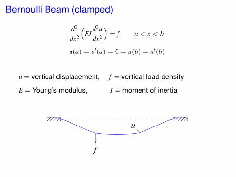
Bernoulli Beam (clamped)
d2
dx2
(EI
d2udx2
)= f a < x < b
u(a) = u′(a) = 0 = u(b) = u′(b)
u = vertical displacement, f = vertical load density
E = Young’s modulus, I = moment of inertia
f
u
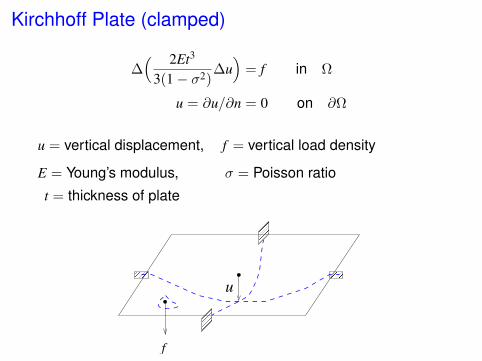
Kirchhoff Plate (clamped)
∆( 2Et3
3(1− σ2)∆u)
= f in Ω
u = ∂u/∂n = 0 on ∂Ω
u = vertical displacement, f = vertical load density
E = Young’s modulus, σ = Poisson ratio
t = thickness of plate
f
u

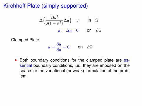
Kirchhoff Plate (simply supported)
∆( 2Et3
3(1− σ2)∆u)
= f in Ω
u = ∆u= 0 on ∂Ω
Clamped Plate
u =∂u∂n
= 0 on ∂Ω
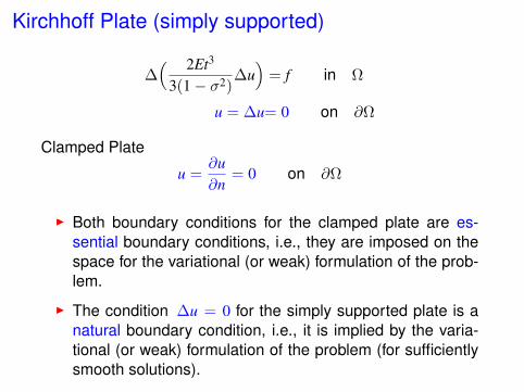
Kirchhoff Plate (simply supported)
∆( 2Et3
3(1− σ2)∆u)
= f in Ω
u = ∆u= 0 on ∂Ω
Clamped Plate
u =∂u∂n
= 0 on ∂Ω
I Both boundary conditions for the clamped plate are es-sential boundary conditions, i.e., they are imposed on thespace for the variational (or weak) formulation of the prob-lem.
Kirchhoff Plate (simply supported)
∆( 2Et3
3(1− σ2)∆u)
= f in Ω
u = ∆u= 0 on ∂Ω
Clamped Plate
u =∂u∂n
= 0 on ∂Ω
I Both boundary conditions for the clamped plate are es-sential boundary conditions, i.e., they are imposed on thespace for the variational (or weak) formulation of the prob-lem.
I The condition ∆u = 0 for the simply supported plate is anatural boundary condition, i.e., it is implied by the varia-tional (or weak) formulation of the problem (for sufficientlysmooth solutions).
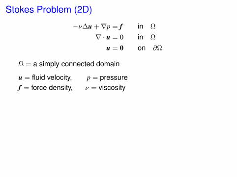
Stokes Problem (2D)
−ν∆u +∇p = f in Ω
∇ · u = 0 in Ω
u = 0 on ∂Ω
Ω = a simply connected domain
u = fluid velocity, p = pressuref = force density, ν = viscosity

Stokes Problem (2D)
−ν∆u +∇p = f in Ω
∇ · u = 0 in Ω
u = 0 on ∂Ω
Ω = a simply connected domain
Stream Function ψ∇× ψ = u

Stokes Problem (2D)
−ν∆u +∇p = f in Ω
∇ · u = 0 in Ω
u = 0 on ∂Ω
Ω = a simply connected domain
Stream Function ψ∇× ψ = u
Boundary value problem for ψ (after simplification)
ν∆2ψ = ∇× f in Ω
ψ = ∂ψ/∂n = 0 on ∂Ω
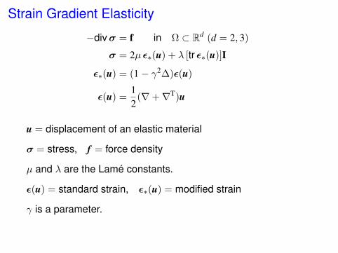
Strain Gradient Elasticity
−divσ = f in Ω ⊂ Rd (d = 2, 3)
σ = 2µ ε∗(u) + λ [tr ε∗(u)]I
ε∗(u) = (1− γ2∆)ε(u)
ε(u) =12
(∇+∇T)u
u = displacement of an elastic material
σ = stress, f = force density
µ and λ are the Lamé constants.
ε(u) = standard strain, ε∗(u) = modified strain
γ is a parameter.
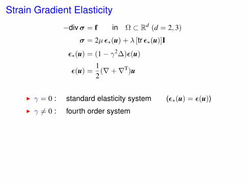
Strain Gradient Elasticity
−divσ = f in Ω ⊂ Rd (d = 2, 3)
σ = 2µ ε∗(u) + λ [tr ε∗(u)]I
ε∗(u) = (1− γ2∆)ε(u)
ε(u) =12
(∇+∇T)u
I γ = 0 : standard elasticity system (ε∗(u) = ε(u))
I γ 6= 0 : fourth order system
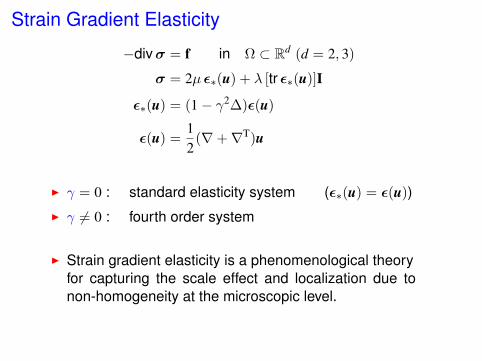
Strain Gradient Elasticity
−divσ = f in Ω ⊂ Rd (d = 2, 3)
σ = 2µ ε∗(u) + λ [tr ε∗(u)]I
ε∗(u) = (1− γ2∆)ε(u)
ε(u) =12
(∇+∇T)u
I γ = 0 : standard elasticity system (ε∗(u) = ε(u))
I γ 6= 0 : fourth order system
I Strain gradient elasticity is a phenomenological theoryfor capturing the scale effect and localization due tonon-homogeneity at the microscopic level.
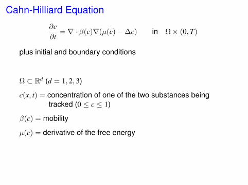
Cahn-Hilliard Equation
∂c∂t
= ∇ · β(c)∇(µ(c)−∆c) in Ω× (0,T)
plus initial and boundary conditions
Ω ⊂ Rd (d = 1, 2, 3)
c(x, t) = concentration of one of the two substances beingtracked (0 ≤ c ≤ 1)
β(c) = mobility
µ(c) = derivative of the free energy
Cahn-Hilliard Equation
∂c∂t
= ∇ · β(c)∇(µ(c)−∆c) in Ω× (0,T)
I phase segregation of binary alloys
I two-phase fluid flow
I image processing
I self-assembly of nanovoids
I planet formation
Cahn-Hilliard Equation
∂c∂t
= ∇ · β(c)∇(µ(c)−∆c) in Ω× (0,T)
This can be solved numerically by an implicit time discretizationcombined with the Newton-Raphson scheme for a fourth ordernonlinear problem at each time step.
An Obstacle Problem
Ω = bounded polygon f ∈ L2(Ω) (external force)
ψ ∈ C2(Ω), ψ < 0 on ∂Ω (obstacle function)
K = v ∈ H20(Ω) : v ≥ ψ on Ω
(v ∈ H20(Ω) if and only if ∂αu/∂xα ∈ L2(Ω) for |α| ≤ 2 and
v = ∂v/∂n = 0 on ∂Ω.)
An Obstacle Problem
Ω = bounded polygon f ∈ L2(Ω) (external force)
ψ ∈ C2(Ω), ψ < 0 on ∂Ω (obstacle function)
K = v ∈ H20(Ω) : v ≥ ψ on Ω
Find u = argminv∈K
[12
a(v, v)− (f , v)]
a(w, v) =
∫Ω
D2w : D2v dx D2w : D2v =
2∑i,j=1
wxixjvxixj
(f , v) =
∫Ω
f v dx
(bending of a clamped Kirchhoff plate over an obstacle)
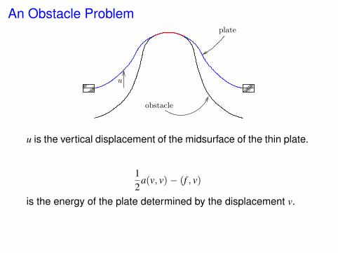
An Obstacle Problem
PSfrag replacementsu
obstacle
plate
u is the vertical displacement of the midsurface of the thin plate.
12
a(v, v)− (f , v)
is the energy of the plate determined by the displacement v.
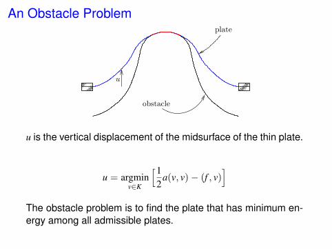
An Obstacle Problem
PSfrag replacementsu
obstacle
plate
u is the vertical displacement of the midsurface of the thin plate.
u = argminv∈K
[12
a(v, v)− (f , v)]
The obstacle problem is to find the plate that has minimum en-ergy among all admissible plates.
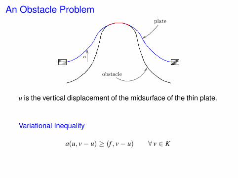
An Obstacle Problem
PSfrag replacementsu
obstacle
plate
u is the vertical displacement of the midsurface of the thin plate.
Variational Inequality
a(u, v− u) ≥ (f , v− u) ∀ v ∈ K
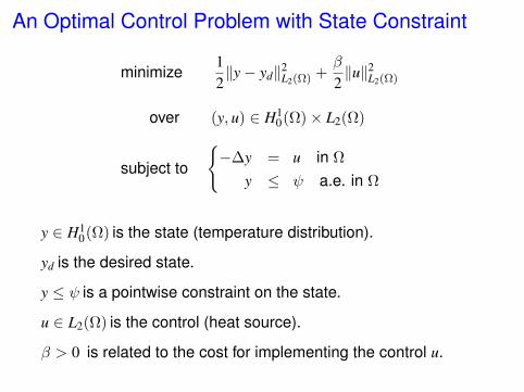
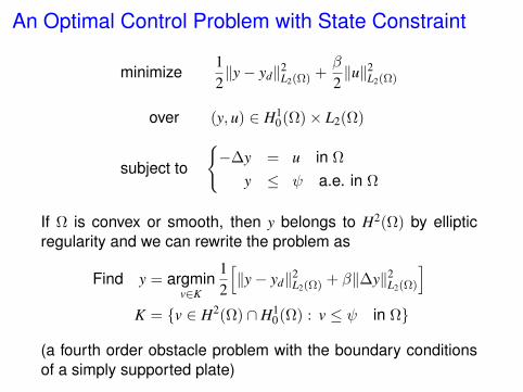
An Optimal Control Problem with State Constraint
minimize12‖y− yd‖2
L2(Ω) +β
2‖u‖2
L2(Ω)
over (y, u) ∈ H10(Ω)× L2(Ω)
subject to
−∆y = u in Ω
y ≤ ψ a.e. in Ω
y ∈ H10(Ω) is the state (temperature distribution).
yd is the desired state.
y ≤ ψ is a pointwise constraint on the state.
u ∈ L2(Ω) is the control (heat source).
β > 0 is related to the cost for implementing the control u.
An Optimal Control Problem with State Constraint
minimize12‖y− yd‖2
L2(Ω) +β
2‖u‖2
L2(Ω)
over (y, u) ∈ H10(Ω)× L2(Ω)
subject to
−∆y = u in Ω
y ≤ ψ a.e. in Ω
If Ω is convex or smooth, then y belongs to H2(Ω) by ellipticregularity and we can rewrite the problem as
Find y = argminv∈K
12
[‖y− yd‖2
L2(Ω) + β‖∆y‖2L2(Ω)
]K = v ∈ H2(Ω) ∩ H1
0(Ω) : v ≤ ψ in Ω
(a fourth order obstacle problem with the boundary conditionsof a simply supported plate)
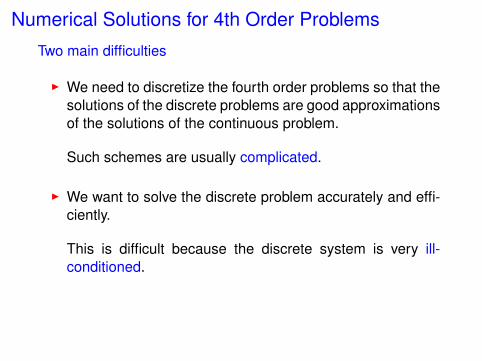
Numerical Solutions for 4th Order Problems
Two main difficulties
I We need to discretize the fourth order problems so that thesolutions of the discrete problems are good approximationsof the solutions of the continuous problem.
Such schemes are usually complicated.
I We want to solve the discrete problem accurately and effi-ciently.
This is difficult because the discrete system is very ill-conditioned.
Classical Finite Element Methods
Conforming Methods
Conforming Methods
Since the continuous problems are posed on the Sobolev spaceH2(Ω), the finite element spaces of conforming methods mustbe subspaces of H2(Ω), i.e., they are C1 finite element spaces.
The advantage of conforming methods is that they are alwaysconvergent by Galerkin orthogonality. The disadvantage is thatthey are complicated in 2D (and more so in 3D).
Conforming Methods
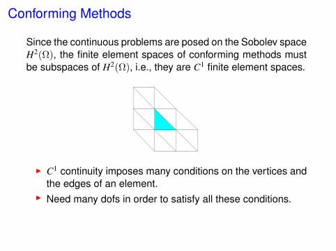
Since the continuous problems are posed on the Sobolev spaceH2(Ω), the finite element spaces of conforming methods mustbe subspaces of H2(Ω), i.e., they are C1 finite element spaces.
I C1 continuity imposes many conditions on the vertices andthe edges of an element.
I Need many dofs in order to satisfy all these conditions.
Conforming Methods
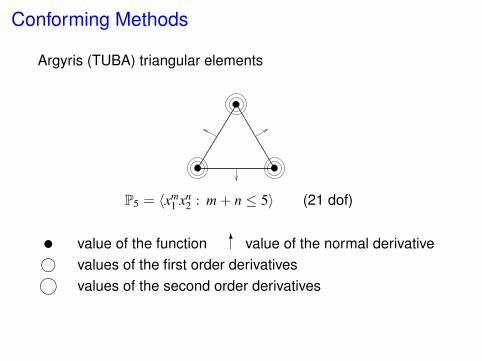
Argyris (TUBA) triangular elements
P5 = 〈xm1 xn
2 : m + n ≤ 5〉 (21 dof)
u value of the function 6value of the normal derivativei values of the first order derivativesk values of the second order derivatives
Conforming Methods
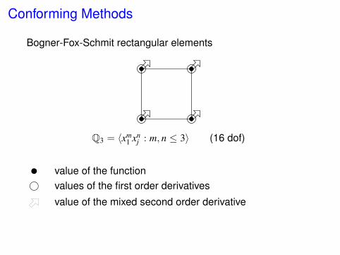
Bogner-Fox-Schmit rectangular elements
Q3 = 〈xm1 xn
j : m, n ≤ 3〉 (16 dof)
u value of the functionh values of the first order derivatives
value of the mixed second order derivative
Conforming Methods
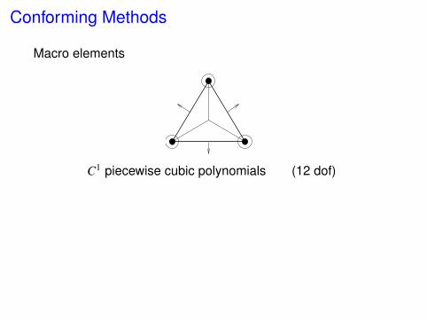
Macro elements
C1 piecewise cubic polynomials (12 dof)

Nonconforming Methods
Nonconforming Methods
Nonconforming finite element methods were invented becauseC1 finite element methods are too complicated. Nonconformingmethods are simpler since we only require the finite elementfunctions and their derivatives to satisfy some weak continuityconditions.
Nonconforming Methods
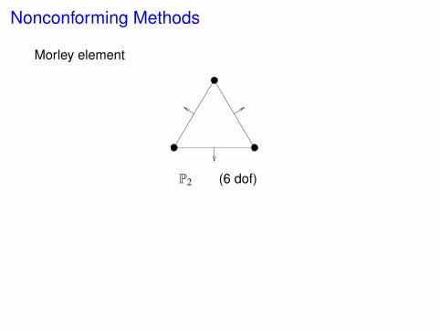
Morley element
P2 (6 dof)
Nonconforming Methods
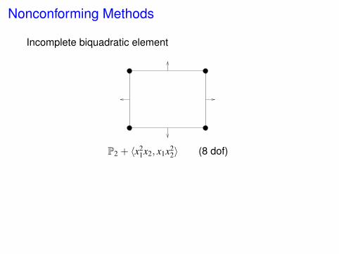
Incomplete biquadratic element
P2 + 〈x21x2, x1x2
2〉 (8 dof)
Nonconforming Methods
I It takes a lot of ingenuity to construct nonconforming finiteelements that work (especially for more complicated fourthorder problems).
I They are only low order elements (no natural hierarchy),which are not efficient for smooth solutions.
I Very little is known about 3D nonconforming elements forfourth order problems.
Mixed Finite Element Methods
Mixed Finite Element Methods
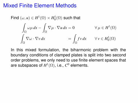
Find (ω, u) ∈ H1(Ω)× H10(Ω) such that∫
Ωωµ dx−
∫Ω∇µ · ∇u dx = 0 ∀µ ∈ H1(Ω)∫
Ω∇ω · ∇v dx =
∫Ω
f v dx ∀ v ∈ H10(Ω)
In this mixed formulation, the biharmonic problem with theboundary conditions of clamped plates is split into two secondorder problems, we only need to use finite element spaces thatare subspaces of H1(Ω), i.e., C0 elements.
Mixed Finite Element Methods
I It is not easy to come up with correct mixed formulationsfor more complicated fourth order problems.
Mixed Finite Element Methods
I It is not easy to come up with correct mixed formulationsfor more complicated fourth order problems.
I In the mixed formulation we use a finite element space forthe unknown ω and a finite element space for the unknownu. The mixed method only works if the finite element pairsatisfies the Ladyzhenskaya-Babuška-Brezzi condition.
It is not easy to find such finite element pairs!
Mixed Finite Element Methods
I It is not easy to come up with correct mixed formulationsfor more complicated fourth order problems.
I In the mixed formulation we use a finite element space forthe unknown ω and a finite element space for the unknownu. The mixed method only works if the finite element pairsatisfies the Ladyzhenskaya-Babuška-Brezzi condition.
I For the biharmonic problem with boundary conditions ofsimply supported plates, some mixed methods can missthe leading singularity and produce a wrong solution(Sapondzhyan paradox).
I At the end one still needs to solve a saddle point problem,which is more complicated than solving an SPD problem.
C0 Interior Penalty Methods
C0 Interior Penalty Methods
The lowest order elements in this family are as simple asthe classical nonconforming finite elements.
C0 Interior Penalty Methods
The lowest order elements in this family are as simple asthe classical nonconforming finite elements.
We can compute smooth solutions using higher order ele-ments in this family which are as efficient as higher orderC1 elements and much simpler (in 2D and 3D).

C0 Interior Penalty Methods
The lowest order elements in this family are as simple asthe classical nonconforming finite elements.
We can compute smooth solutions using higher order ele-ments in this family which are as efficient as higher orderC1 elements and much simpler (in 2D and 3D).
Unlike mixed methods, this approach can be extended ina straight-forward way to more complicated fourth orderproblems (such as the fourth order elliptic systems that ap-pear in strain-gradient elasticity problems).
The C0 interior penalty methods belong to the class of dis-continuous Galerkin methods (where the discontinuity in-volves the first order derivatives).
C0 Interior Penalty Methods
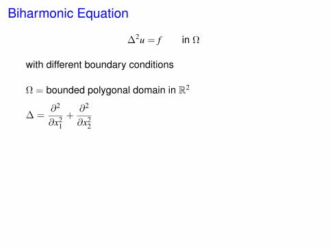
Biharmonic Equation
∆2u = f in Ω
with different boundary conditions
Ω = bounded polygonal domain in R2
∆ =∂2
∂x21
+∂2
∂x22
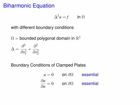
Biharmonic Equation
∆2u = f in Ω
with different boundary conditions
Ω = bounded polygonal domain in R2
∆ =∂2
∂x21
+∂2
∂x22
Boundary Conditions of Clamped Plates
u = 0 on ∂Ω essential∂u∂n
= 0 on ∂Ω essential
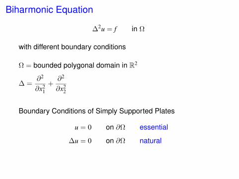
Biharmonic Equation
∆2u = f in Ω
with different boundary conditions
Ω = bounded polygonal domain in R2
∆ =∂2
∂x21
+∂2
∂x22
Boundary Conditions of Simply Supported Plates
u = 0 on ∂Ω essential
∆u = 0 on ∂Ω natural

Biharmonic Equation
∆2u = f in Ω
with different boundary conditions
Ω = bounded polygonal domain in R2
∆ =∂2
∂x21
+∂2
∂x22
Boundary Conditions of the Cahn-Hilliard Type
∂u∂n
= 0 on ∂Ω essential
∂(∆u)
∂n= 0 on ∂Ω natural
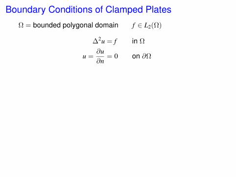
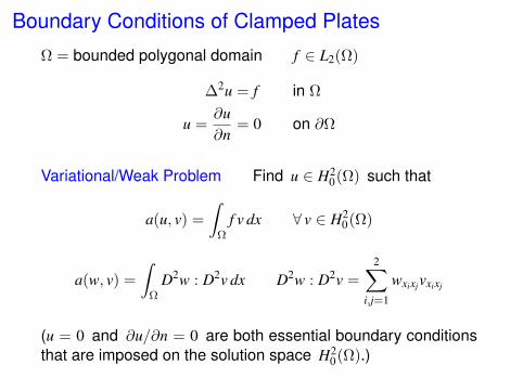
Boundary Conditions of Clamped Plates
Ω = bounded polygonal domain f ∈ L2(Ω)
∆2u = f in Ω
u =∂u∂n
= 0 on ∂Ω
Boundary Conditions of Clamped Plates
Ω = bounded polygonal domain f ∈ L2(Ω)
∆2u = f in Ω
u =∂u∂n
= 0 on ∂Ω
Variational/Weak Problem Find u ∈ H20(Ω) such that
a(u, v) =
∫Ω
f v dx ∀ v ∈ H20(Ω)
a(w, v) =
∫Ω
D2w : D2v dx D2w : D2v =
2∑i,j=1
wxixjvxixj
(u = 0 and ∂u/∂n = 0 are both essential boundary conditionsthat are imposed on the solution space H2
0(Ω).)
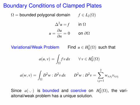
Boundary Conditions of Clamped Plates
Ω = bounded polygonal domain f ∈ L2(Ω)
∆2u = f in Ω
u =∂u∂n
= 0 on ∂Ω
Variational/Weak Problem Find u ∈ H20(Ω) such that
a(u, v) =
∫Ω
f v dx ∀ v ∈ H20(Ω)
a(w, v) =
∫Ω
D2w : D2v dx D2w : D2v =
2∑i,j=1
wxixjvxixj
Since a(·, ·) is bounded and coercive on H20(Ω), the vari-
aitonal/weak problem has a unique solution.

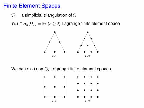
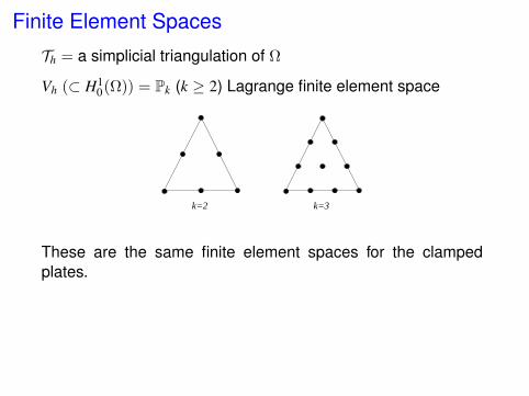
Finite Element Spaces
Th = a simplicial triangulation of Ω
Vh (⊂ H10(Ω)) = Pk (k ≥ 2) Lagrange finite element space
k=3k=2
Finite Element Spaces
Th = a simplicial triangulation of Ω
Vh (⊂ H10(Ω)) = Pk (k ≥ 2) Lagrange finite element space
k=3k=2
We can also use Qk Lagrange finite element spaces.
k=3k=2
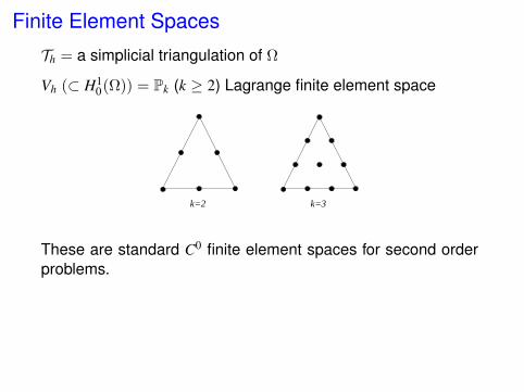
Finite Element Spaces
Th = a simplicial triangulation of Ω
Vh (⊂ H10(Ω)) = Pk (k ≥ 2) Lagrange finite element space
k=3k=2
These are standard C0 finite element spaces for second orderproblems.
Discrete Problem

Discrete Problem
Key Observation The solution u of the continuous problem
a(u, v) =
∫Ω
f v dx ∀ v ∈ H20(Ω)
a(w, v) =
∫Ω
D2w : D2v dx
f ∈ L2(Ω)
also satisfies a mesh-dependent problem
ah(u, v) =
∫Ω
f v dx ∀ v ∈ Vh
obtained by
I integration by parts
I symmetrization
I stabilization
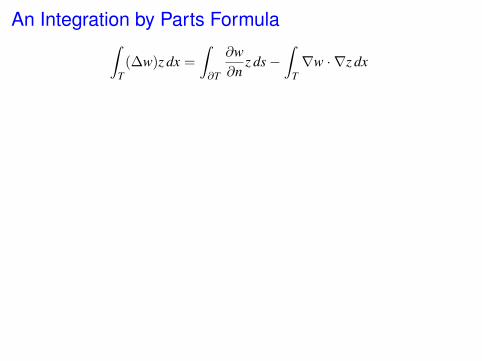
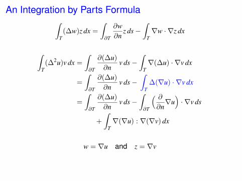
An Integration by Parts Formula∫T(∆w)z dx =
∫∂T
∂w∂n
z ds−∫
T∇w · ∇z dx
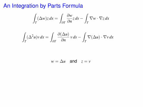
An Integration by Parts Formula∫T(∆w)z dx =
∫∂T
∂w∂n
z ds−∫
T∇w · ∇z dx
∫T(∆2u)v dx =
∫∂T
∂(∆u)
∂nv ds−
∫T∇(∆u) · ∇v dx
w = ∆u and z = v
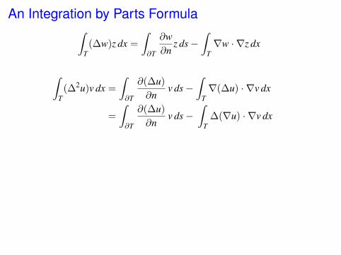
An Integration by Parts Formula∫T(∆w)z dx =
∫∂T
∂w∂n
z ds−∫
T∇w · ∇z dx
∫T(∆2u)v dx =
∫∂T
∂(∆u)
∂nv ds−
∫T∇(∆u) · ∇v dx
=
∫∂T
∂(∆u)
∂nv ds−
∫T
∆(∇u) · ∇v dx
An Integration by Parts Formula∫T(∆w)z dx =
∫∂T
∂w∂n
z ds−∫
T∇w · ∇z dx
∫T(∆2u)v dx =
∫∂T
∂(∆u)
∂nv ds−
∫T∇(∆u) · ∇v dx
=
∫∂T
∂(∆u)
∂nv ds−
∫T
∆(∇u) · ∇v dx
=
∫∂T
∂(∆u)
∂nv ds−
∫∂T
( ∂∂n∇u)· ∇v ds
+
∫T∇(∇u) : ∇(∇v) dx
w = ∇u and z = ∇v
An Integration by Parts Formula∫T(∆w)z dx =
∫∂T
∂w∂n
z ds−∫
T∇w · ∇z dx
∫T(∆2u)v dx =
∫∂T
∂(∆u)
∂nv ds−
∫T∇(∆u) · ∇v dx
=
∫∂T
∂(∆u)
∂nv ds−
∫T
∆(∇u) · ∇v dx
=
∫∂T
∂(∆u)
∂nv ds−
∫∂T
( ∂∂n∇u)· ∇v ds
+
∫T∇(∇u) : ∇(∇v) dx
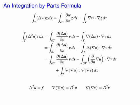
∆2u = f ∇(∇u) = D2u ∇(∇v) = D2v
An Integration by Parts Formula∫T(∆w)z dx =
∫∂T
∂w∂n
z ds−∫
T∇w · ∇z dx
∫T(∆2u)v dx =
∫∂T
∂(∆u)
∂nv ds−
∫T∇(∆u) · ∇v dx
=
∫∂T
∂(∆u)
∂nv ds−
∫T
∆(∇u) · ∇v dx
=
∫∂T
∂(∆u)
∂nv ds−
∫∂T
( ∂∂n∇u)· ∇v ds
+
∫T∇(∇u) : ∇(∇v) dx
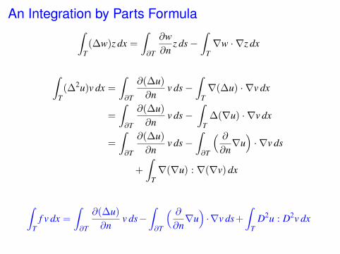
∫T
f v dx =
∫∂T
∂(∆u)
∂nv ds−
∫∂T
( ∂∂n∇u)·∇v ds +
∫T
D2u : D2v dx
Notation
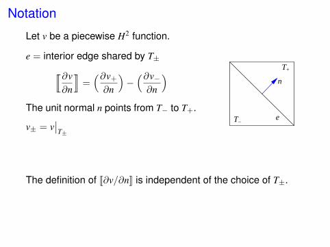
Let v be a piecewise H2 function.
e = interior edge shared by T±[[∂v∂n
]]=(∂v+
∂n
)−(∂v−∂n
)The unit normal n points from T− to T+.
v± = v∣∣T±
T
e
+
T_
n
The definition of [[∂v/∂n]] is independent of the choice of T±.

Notation
Let v be a piecewise H2 function.
e = interior edge shared by T±[[∂v∂n
]]=(∂v+
∂n
)−(∂v−∂n
)The unit normal n points from T− to T+.
v± = v∣∣T±
T
e
+
T_
n
e = boundary edge, e ⊂ ∂T[[∂v∂n
]]= −∂vT
∂n
The unit normal n points outside Ω.
vT = v∣∣T
T
ne
Notation
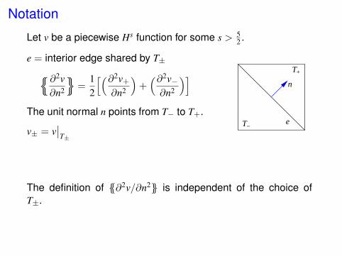
Let v be a piecewise Hs function for some s > 52 .
e = interior edge shared by T±∂2v∂n2
=
12
[(∂2v+
∂n2
)+(∂2v−∂n2
)]The unit normal n points from T− to T+.
v± = v∣∣T±
T
e
+
T_
n
The definition of ∂2v/∂n2 is independent of the choice ofT±.
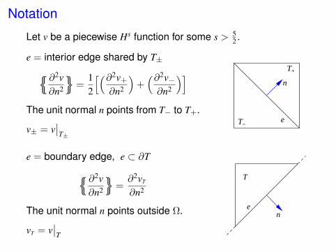
Notation
Let v be a piecewise Hs function for some s > 52 .
e = interior edge shared by T±∂2v∂n2
=
12
[(∂2v+
∂n2
)+(∂2v−∂n2
)]The unit normal n points from T− to T+.
v± = v∣∣T±
T
e
+
T_
n
e = boundary edge, e ⊂ ∂T∂2v∂n2
=∂2vT
∂n2
The unit normal n points outside Ω.
vT = v∣∣T
T
ne

A Mesh-Dependent Problem for u
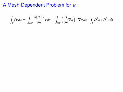
A Mesh-Dependent Problem for u
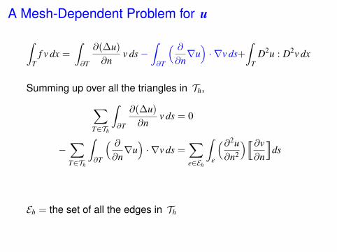
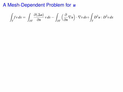
∫T
f v dx =
∫∂T
∂(∆u)
∂nv ds−
∫∂T
( ∂∂n∇u)· ∇v ds+
∫T
D2u : D2v dx
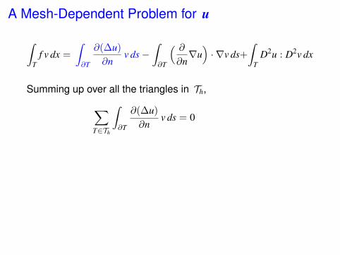
A Mesh-Dependent Problem for u
∫T
f v dx =
∫∂T
∂(∆u)
∂nv ds−
∫∂T
( ∂∂n∇u)· ∇v ds+
∫T
D2u : D2v dx
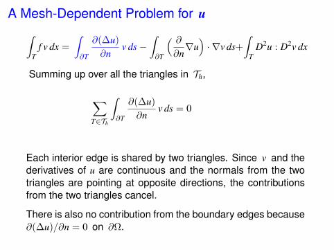
Summing up over all the triangles in Th,∑T∈Th
∫∂T
∂(∆u)
∂nv ds = 0

A Mesh-Dependent Problem for u
∫T
f v dx =
∫∂T
∂(∆u)
∂nv ds−
∫∂T
( ∂∂n∇u)· ∇v ds+
∫T
D2u : D2v dx
Summing up over all the triangles in Th,∑T∈Th
∫∂T
∂(∆u)
∂nv ds = 0
Each interior edge is shared by two triangles. Since v and thederivatives of u are continuous and the normals from the twotriangles are pointing at opposite directions, the contributionsfrom the two triangles cancel.
There is also no contribution from the boundary edges becausev = 0 on ∂Ω.
A Mesh-Dependent Problem for u
∫T
f v dx =
∫∂T
∂(∆u)
∂nv ds−
∫∂T
( ∂∂n∇u)· ∇v ds+
∫T
D2u : D2v dx
Summing up over all the triangles in Th,∑T∈Th
∫∂T
∂(∆u)
∂nv ds = 0
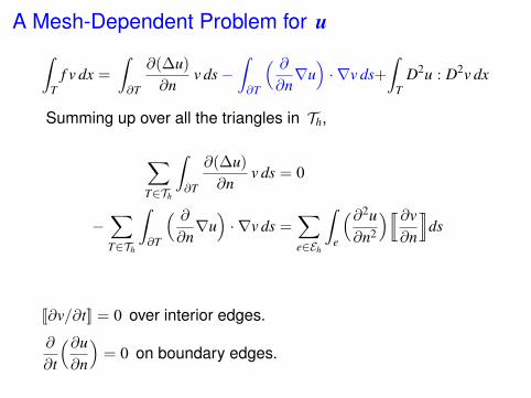
−∑T∈Th
∫∂T
( ∂∂n∇u)· ∇v ds =
∑e∈Eh
∫e
(∂2u∂n2
)[[∂v∂n
]]ds
Eh = the set of all the edges in Th
A Mesh-Dependent Problem for u
∫T
f v dx =
∫∂T
∂(∆u)
∂nv ds−
∫∂T
( ∂∂n∇u)· ∇v ds+
∫T
D2u : D2v dx
Summing up over all the triangles in Th,∑T∈Th
∫∂T
∂(∆u)
∂nv ds = 0
−∑T∈Th
∫∂T
( ∂∂n∇u)· ∇v ds =
∑e∈Eh
∫e
(∂2u∂n2
)[[∂v∂n
]]ds
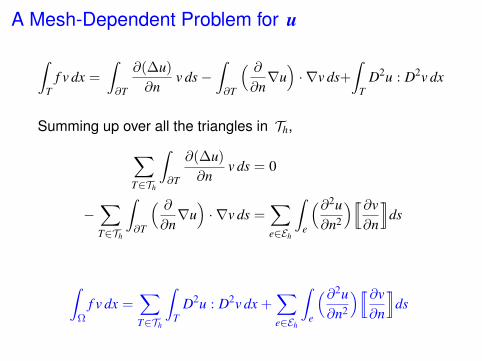
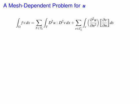
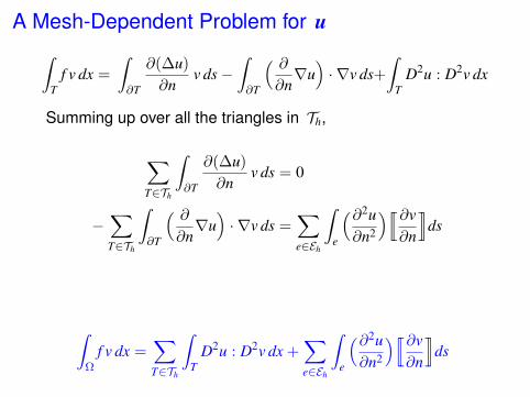
∫Ω
f v dx =∑T∈Th
∫T
D2u : D2v dx +∑e∈Eh
∫e
(∂2u∂n2
)[[∂v∂n
]]ds
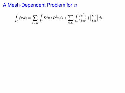
A Mesh-Dependent Problem for u∫
Ωf v dx =
∑T∈Th
∫T
D2u : D2v dx +∑e∈Eh
∫e
(∂2u∂n2
)[[∂v∂n
]]ds
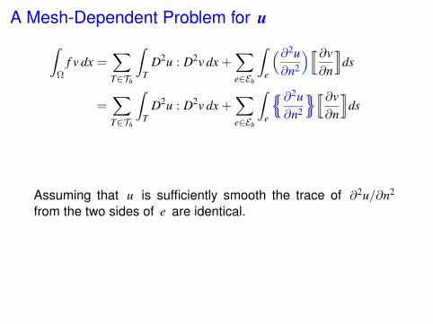
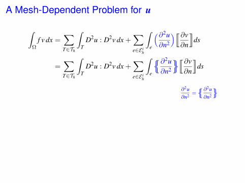
A Mesh-Dependent Problem for u∫
Ωf v dx =
∑T∈Th
∫T
D2u : D2v dx +∑e∈Eh
∫e
(∂2u∂n2
)[[∂v∂n
]]ds
=∑T∈Th
∫T
D2u : D2v dx +∑e∈Eh
∫e
∂2u∂n2
[[∂v∂n
]]ds
Assuming that u is sufficiently smooth the trace of ∂2u/∂n2
from the two sides of e are identical.
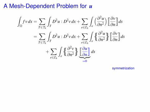
A Mesh-Dependent Problem for u∫
Ωf v dx =
∑T∈Th
∫T
D2u : D2v dx +∑e∈Eh
∫e
(∂2u∂n2
)[[∂v∂n
]]ds
=∑T∈Th
∫T
D2u : D2v dx +∑e∈Eh
∫e
∂2u∂n2
[[∂v∂n
]]ds
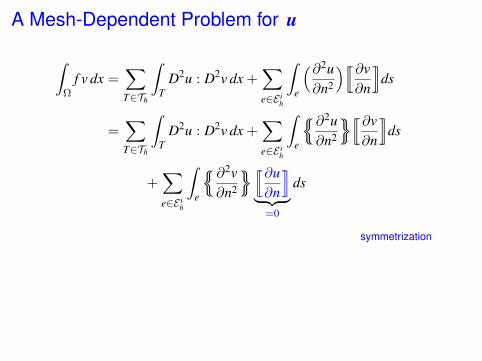
+∑e∈Eh
∫e
∂2v∂n2
[[∂u∂n
]]︸ ︷︷ ︸
=0
ds
symmetrization
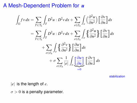
A Mesh-Dependent Problem for u∫
Ωf v dx =
∑T∈Th
∫T
D2u : D2v dx +∑e∈Eh
∫e
(∂2u∂n2
)[[∂v∂n
]]ds
=∑T∈Th
∫T
D2u : D2v dx +∑e∈Eh
∫e
∂2u∂n2
[[∂v∂n
]]ds
+∑e∈Eh
∫e
∂2v∂n2
[[∂u∂n
]]ds
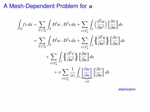
+ σ∑e∈Eh
1|e|
∫e
[[∂u∂n
]]︸ ︷︷ ︸
=0
[[∂v∂n
]]ds
stabilization
|e| is the length of e.
σ > 0 is a penalty parameter.
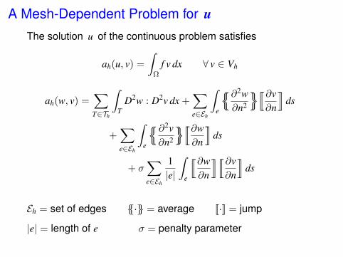
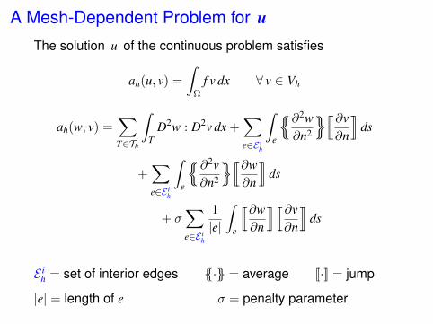
A Mesh-Dependent Problem for uThe solution u of the continuous problem satisfies
ah(u, v) =
∫Ω
f v dx ∀ v ∈ Vh
ah(w, v) =∑T∈Th
∫T
D2w : D2v dx +∑e∈Eh
∫e
∂2w∂n2
[[∂v∂n
]]ds
+∑e∈Eh
∫e
∂2v∂n2
[[∂w∂n
]]ds
+ σ∑e∈Eh
1|e|
∫e
[[∂w∂n
]][[∂v∂n
]]ds
Eh = set of edges · = average [[·]] = jump
|e| = length of e σ = penalty parameter
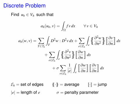
Discrete Problem
Find uh ∈ Vh such that
ah(uh, v) =
∫Ω
f v dx ∀ v ∈ Vh
ah(w, v) =∑T∈Th
∫T
D2w : D2v dx +∑e∈Eh
∫e
∂2w∂n2
[[∂v∂n
]]ds
+∑e∈Eh
∫e
∂2v∂n2
[[∂w∂n
]]ds
+ σ∑e∈Eh
1|e|
∫e
[[∂w∂n
]][[∂v∂n
]]ds
Eh = set of edges · = average [[·]] = jump
|e| = length of e σ = penalty parameter

Discrete Problem
Find uh ∈ Vh such that
ah(uh, v) =
∫Ω
f v dx ∀ v ∈ Vh
Galerkin Orthogonality
ah(u, v) =
∫Ω
fv dx ∀ v ∈ Vh
ah(uh, v) =
∫Ω
fv dx ∀ v ∈ Vh
ah(u− uh, v) = 0 ∀ v ∈ Vh
Discrete Problem
This is an interior penalty method obtained through integrationby parts, symmetrization and stabilization.
Discrete Problem
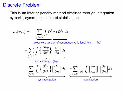
This is an interior penalty method obtained through integrationby parts, symmetrization and stabilization.
ah(w, v) =∑T∈Th
∫T
D2w : D2v dx︸ ︷︷ ︸piecewise version of continuous variational form (ibp)
+∑e∈Eh
∫e
∂2w∂n2
[[∂v∂n
]]ds︸ ︷︷ ︸
consistency (ibp)
+∑e∈Eh
∫e
∂2v∂n2
[[∂w∂n
]]ds︸ ︷︷ ︸
symmetrization
+σ∑e∈Eh
1|e|
∫e
[[∂w∂n
]] [[∂v∂n
]]ds︸ ︷︷ ︸
stabilization
Discrete Problem
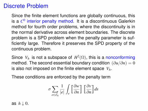
Since the finite element functions are globally continuous, thisis a C0 interior penalty method. It is a discontinuous Galerkinmethod for fourth order problems, where the discontinuity is inthe normal derivative across element boundaries. The discreteproblem is a SPD problem when the penalty parameter is suf-ficiently large. Therefore it preserves the SPD property of thecontinuous problem.
Discrete Problem
Since the finite element functions are globally continuous, thisis a C0 interior penalty method. It is a discontinuous Galerkinmethod for fourth order problems, where the discontinuity is inthe normal derivative across element boundaries. The discreteproblem is a SPD problem when the penalty parameter is suf-ficiently large. Therefore it preserves the SPD property of thecontinuous problem.
Since Vh is not a subspace of H2(Ω), this is a nonconformingmethod. The second essential boundary condition (∂u/∂n) = 0is also not imposed on the finite element space Vh.
These conditions are enforced by the penalty term
σ∑e∈Eh
1|e|
∫e
[[∂w∂n
]] [[∂v∂n
]]ds
as h ↓ 0.
Discrete Problem
Since the finite element functions are globally continuous, thisis a C0 interior penalty method. It is a discontinuous Galerkinmethod for fourth order problems, where the discontinuity is inthe normal derivative across element boundaries. The discreteproblem is a SPD problem when the penalty parameter is suf-ficiently large. Therefore it preserves the SPD property of thecontinuous problem.
The study of discontinuous Galerkin methods for higher orderproblems was initiated in a paper by Baker.
ReferenceBaker
Finite element methods for elliptic equations using nonconforming elements
Math. Comp. 1977

Discrete Problem
Since the finite element functions are globally continuous, thisis a C0 interior penalty method. It is a discontinuous Galerkinmethod for fourth order problems, where the discontinuity is inthe normal derivative across element boundaries. The discreteproblem is a SPD problem when the penalty parameter is suf-ficiently large. Therefore it preserves the SPD property of thecontinuous problem.
ReferenceEngel, Garikipati, Hughes, Larson, Mazzei, and Taylor
Continuous/discontinuous finite element approximations of fourth order el-liptic problems in structural and continuum mechanics with applications tothin beams and plates, and strain gradient elasticity
Comput. Methods Appl. Mech. Engrg. 2002
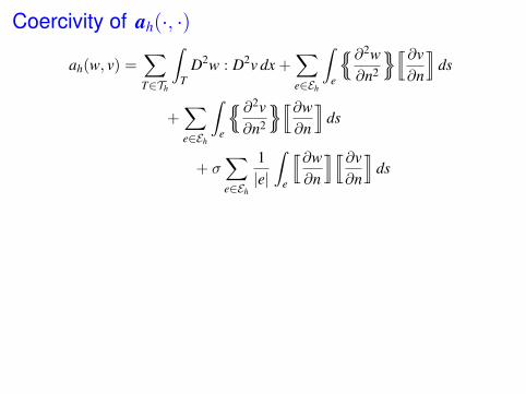
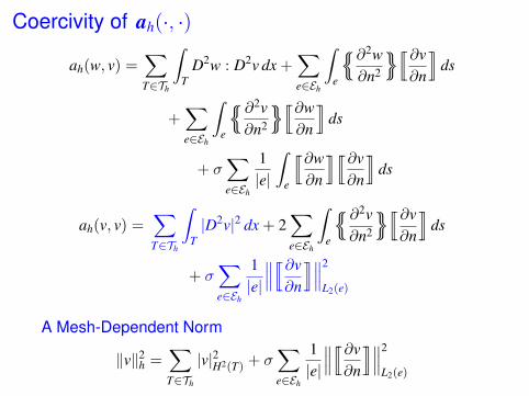
Coercivity of ah(·, ·)
ah(w, v) =∑T∈Th
∫T
D2w : D2v dx +∑e∈Eh
∫e
∂2w∂n2
[[∂v∂n
]]ds
+∑e∈Eh
∫e
∂2v∂n2
[[∂w∂n
]]ds
+ σ∑e∈Eh
1|e|
∫e
[[∂w∂n
]][[∂v∂n
]]ds
Coercivity of ah(·, ·)
ah(w, v) =∑T∈Th
∫T
D2w : D2v dx +∑e∈Eh
∫e
∂2w∂n2
[[∂v∂n
]]ds
+∑e∈Eh
∫e
∂2v∂n2
[[∂w∂n
]]ds
+ σ∑e∈Eh
1|e|
∫e
[[∂w∂n
]][[∂v∂n
]]ds
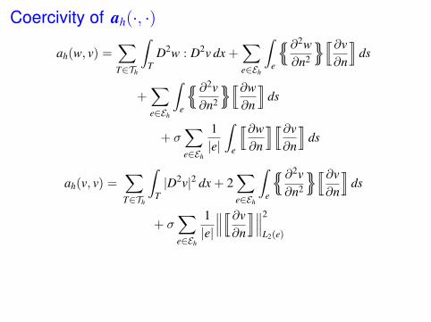
ah(v, v) =∑T∈Th
∫T|D2v|2 dx + 2
∑e∈Eh
∫e
∂2v∂n2
[[∂v∂n
]]ds
+ σ∑e∈Eh
1|e|
∥∥∥[[∂v∂n
]]∥∥∥2
L2(e)
Coercivity of ah(·, ·)
ah(w, v) =∑T∈Th
∫T
D2w : D2v dx +∑e∈Eh
∫e
∂2w∂n2
[[∂v∂n
]]ds
+∑e∈Eh
∫e
∂2v∂n2
[[∂w∂n
]]ds
+ σ∑e∈Eh
1|e|
∫e
[[∂w∂n
]][[∂v∂n
]]ds
ah(v, v) =∑T∈Th
∫T|D2v|2 dx + 2
∑e∈Eh
∫e
∂2v∂n2
[[∂v∂n
]]ds
+ σ∑e∈Eh
1|e|
∥∥∥[[∂v∂n
]]∥∥∥2
L2(e)
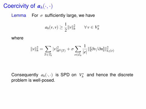
A Mesh-Dependent Norm
‖v‖2h =
∑T∈Th
|v|2H2(T) + σ∑e∈Eh
1|e|
∥∥∥[[∂v∂n
]]∥∥∥2
L2(e)
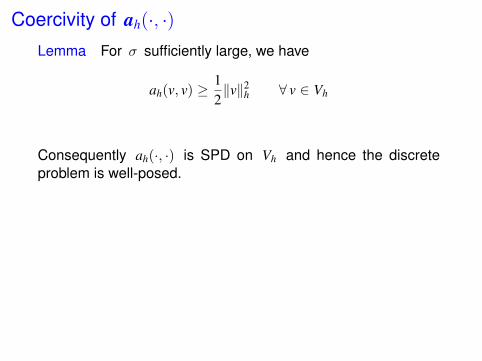
Coercivity of ah(·, ·)Lemma For σ sufficiently large, we have
ah(v, v) ≥ 12‖v‖2
h ∀ v ∈ Vh
Consequently ah(·, ·) is SPD on Vh and hence the discreteproblem is well-posed.
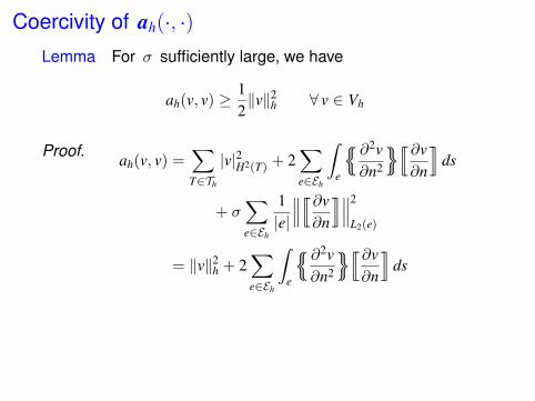
Coercivity of ah(·, ·)Lemma For σ sufficiently large, we have
ah(v, v) ≥ 12‖v‖2
h ∀ v ∈ Vh
Proof. ah(v, v) =∑T∈Th
|v|2H2(T) + 2∑e∈Eh
∫e
∂2v∂n2
[[∂v∂n
]]ds
+ σ∑e∈Eh
1|e|
∥∥∥[[∂v∂n
]]∥∥∥2
L2(e)
= ‖v‖2h + 2
∑e∈Eh
∫e
∂2v∂n2
[[∂v∂n
]]ds
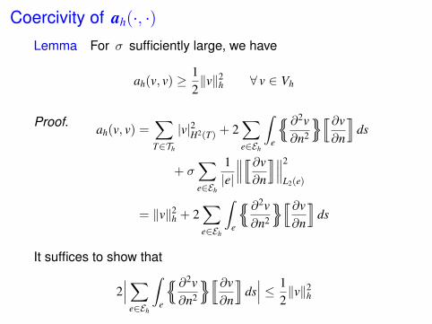
Coercivity of ah(·, ·)Lemma For σ sufficiently large, we have
ah(v, v) ≥ 12‖v‖2
h ∀ v ∈ Vh
Proof. ah(v, v) =∑T∈Th
|v|2H2(T) + 2∑e∈Eh
∫e
∂2v∂n2
[[∂v∂n
]]ds
+ σ∑e∈Eh
1|e|
∥∥∥[[∂v∂n
]]∥∥∥2
L2(e)
= ‖v‖2h + 2
∑e∈Eh
∫e
∂2v∂n2
[[∂v∂n
]]ds
It suffices to show that
2∣∣∣∑
e∈Eh
∫e
∂2v∂n2
[[∂v∂n
]]ds∣∣∣ ≤ 1
2‖v‖2
h

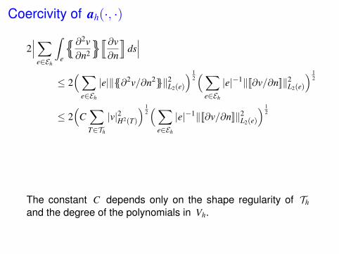
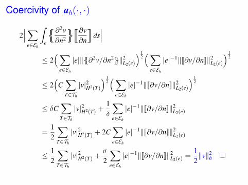
Coercivity of ah(·, ·)
2∣∣∣∑
e∈Eh
∫e
∂2v∂n2
[[∂v∂n
]]ds∣∣∣
≤ 2(∑
e∈Eh
|e|‖∂2v/∂n2‖2L2(e)
) 12(∑
e∈Eh
|e|−1‖[[∂v/∂n]]‖2L2(e)
) 12
∣∣∣ ∫ fg∣∣∣ ≤ (∫ f 2
) 12(∫
g2) 1
2
∣∣∣∑ anbn
∣∣∣ ≤ (∑ a2n
) 12(∑
b2n
) 12
Coercivity of ah(·, ·)
2∣∣∣∑
e∈Eh
∫e
∂2v∂n2
[[∂v∂n
]]ds∣∣∣
≤ 2(∑
e∈Eh
|e|‖∂2v/∂n2‖2L2(e)
) 12(∑
e∈Eh
|e|−1‖[[∂v/∂n]]‖2L2(e)
) 12
≤ 2(
C∑T∈Th
|v|2H2(T)
) 12(∑
e∈Eh
|e|−1‖[[∂v/∂n]]‖2L2(e)
) 12
The constant C depends only on the shape regularity of Th
and the degree of the polynomials in Vh.
Coercivity of ah(·, ·)
2∣∣∣∑
e∈Eh
∫e
∂2v∂n2
[[∂v∂n
]]ds∣∣∣
≤ 2(∑
e∈Eh
|e|‖∂2v/∂n2‖2L2(e)
) 12(∑
e∈Eh
|e|−1‖[[∂v/∂n]]‖2L2(e)
) 12
≤ 2(
C∑T∈Th
|v|2H2(T)
) 12(∑
e∈Eh
|e|−1‖[[∂v/∂n]]‖2L2(e)
) 12
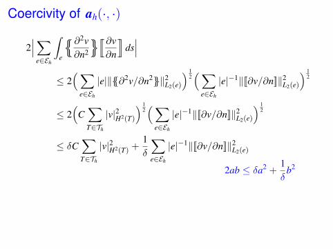
≤ δC∑T∈Th
|v|2H2(T) +1δ
∑e∈Eh
|e|−1‖[[∂v/∂n]]‖2L2(e)
2ab ≤ δa2 +1δ
b2
Coercivity of ah(·, ·)
2∣∣∣∑
e∈Eh
∫e
∂2v∂n2
[[∂v∂n
]]ds∣∣∣
≤ 2(∑
e∈Eh
|e|‖∂2v/∂n2‖2L2(e)
) 12(∑
e∈Eh
|e|−1‖[[∂v/∂n]]‖2L2(e)
) 12
≤ 2(
C∑T∈Th
|v|2H2(T)
) 12(∑
e∈Eh
|e|−1‖[[∂v/∂n]]‖2L2(e)
) 12
≤ δC∑T∈Th
|v|2H2(T) +1δ
∑e∈Eh
|e|−1‖[[∂v/∂n]]‖2L2(e)
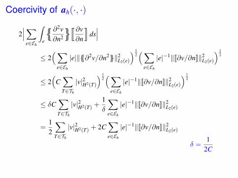
=12
∑T∈Th
|v|2H2(T) + 2C∑e∈Eh
|e|−1‖[[∂v/∂n]]‖2L2(e)
δ =1
2C
Coercivity of ah(·, ·)
2∣∣∣∑
e∈Eh
∫e
∂2v∂n2
[[∂v∂n
]]ds∣∣∣
≤ 2(∑
e∈Eh
|e|‖∂2v/∂n2‖2L2(e)
) 12(∑
e∈Eh
|e|−1‖[[∂v/∂n]]‖2L2(e)
) 12
≤ 2(
C∑T∈Th
|v|2H2(T)
) 12(∑
e∈Eh
|e|−1‖[[∂v/∂n]]‖2L2(e)
) 12
≤ δC∑T∈Th
|v|2H2(T) +1δ
∑e∈Eh
|e|−1‖[[∂v/∂n]]‖2L2(e)
=12
∑T∈Th
|v|2H2(T) + 2C∑e∈Eh
|e|−1‖[[∂v/∂n]]‖2L2(e)
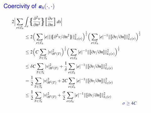
≤ 12
∑T∈Th
|v|2H2(T) +σ
2
∑e∈Eh
|e|−1‖[[∂v/∂n]]‖2L2(e)
σ ≥ 4C
Coercivity of ah(·, ·)
2∣∣∣∑
e∈Eh
∫e
∂2v∂n2
[[∂v∂n
]]ds∣∣∣
≤ 2(∑
e∈Eh
|e|‖∂2v/∂n2‖2L2(e)
) 12(∑
e∈Eh
|e|−1‖[[∂v/∂n]]‖2L2(e)
) 12
≤ 2(
C∑T∈Th
|v|2H2(T)
) 12(∑
e∈Eh
|e|−1‖[[∂v/∂n]]‖2L2(e)
) 12
≤ δC∑T∈Th
|v|2H2(T) +1δ
∑e∈Eh
|e|−1‖[[∂v/∂n]]‖2L2(e)
=12
∑T∈Th
|v|2H2(T) + 2C∑e∈Eh
|e|−1‖[[∂v/∂n]]‖2L2(e)
≤ 12
∑T∈Th
|v|2H2(T) +σ
2
∑e∈Eh
|e|−1‖[[∂v/∂n]]‖2L2(e) =
12‖v‖2
h
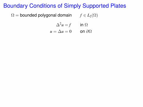
Boundary Conditions of Simply Supported Plates
Ω = bounded polygonal domain f ∈ L2(Ω)
∆2u = f in Ω
u = ∆u = 0 on ∂Ω
Boundary Conditions of Simply Supported Plates
Ω = bounded polygonal domain f ∈ L2(Ω)
∆2u = f in Ω
u = ∆u = 0 on ∂Ω
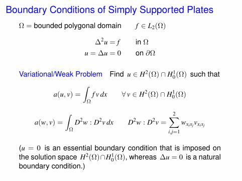
Variational/Weak Problem Find u ∈ H2(Ω) ∩ H10(Ω) such that
a(u, v) =
∫Ω
f v dx ∀ v ∈ H2(Ω) ∩ H10(Ω)
a(w, v) =
∫Ω
D2w : D2v dx D2w : D2v =
2∑i,j=1
wxixjvxixj
(u = 0 is an essential boundary condition that is imposed onthe solution space H2(Ω)∩H1
0(Ω), whereas ∆u = 0 is a naturalboundary condition.)
Boundary Conditions of Simply Supported Plates
Ω = bounded polygonal domain f ∈ L2(Ω)
∆2u = f in Ω
u = ∆u = 0 on ∂Ω
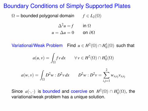
Variational/Weak Problem Find u ∈ H2(Ω) ∩ H10(Ω) such that
a(u, v) =
∫Ω
f v dx ∀ v ∈ H2(Ω) ∩ H10(Ω)
a(w, v) =
∫Ω
D2w : D2v dx D2w : D2v =
2∑i,j=1
wxixjvxixj
Since a(·, ·) is bounded and coercive on H2(Ω) ∩ H10(Ω), the
variational/weak problem has a unique solution.

Finite Element Spaces
Th = a simplicial triangulation of Ω
Vh (⊂ H10(Ω)) = Pk (k ≥ 2) Lagrange finite element space
k=3k=2
We can also use Qk Lagrange finite element spaces.
k=3k=2
Finite Element Spaces
Th = a simplicial triangulation of Ω
Vh (⊂ H10(Ω)) = Pk (k ≥ 2) Lagrange finite element space
k=3k=2
These are the same finite element spaces for the clampedplates.
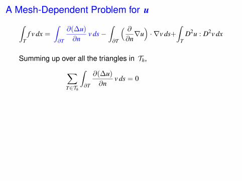
A Mesh-Dependent Problem for u

A Mesh-Dependent Problem for u∫T
f v dx =
∫∂T
∂(∆u)
∂nv ds−
∫∂T
( ∂∂n∇u)· ∇v ds+
∫T
D2u : D2v dx
A Mesh-Dependent Problem for u∫T
f v dx =
∫∂T
∂(∆u)
∂nv ds−
∫∂T
( ∂∂n∇u)· ∇v ds+
∫T
D2u : D2v dx
Summing up over all the triangles in Th,∑T∈Th
∫∂T
∂(∆u)
∂nv ds = 0

A Mesh-Dependent Problem for u∫T
f v dx =
∫∂T
∂(∆u)
∂nv ds−
∫∂T
( ∂∂n∇u)· ∇v ds+
∫T
D2u : D2v dx
Summing up over all the triangles in Th,∑T∈Th
∫∂T
∂(∆u)
∂nv ds = 0
−∑T∈Th
∫∂T
( ∂∂n∇u)· ∇v ds =
∑e∈Eh
∫e
(∂2u∂n2
)[[∂v∂n
]]ds
(Eh = the set of all the edges in Th)
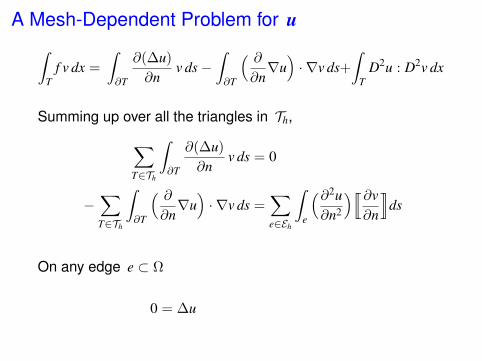
A Mesh-Dependent Problem for u∫T
f v dx =
∫∂T
∂(∆u)
∂nv ds−
∫∂T
( ∂∂n∇u)· ∇v ds+
∫T
D2u : D2v dx
Summing up over all the triangles in Th,∑T∈Th
∫∂T
∂(∆u)
∂nv ds = 0
−∑T∈Th
∫∂T
( ∂∂n∇u)· ∇v ds =
∑e∈Eh
∫e
(∂2u∂n2
)[[∂v∂n
]]ds
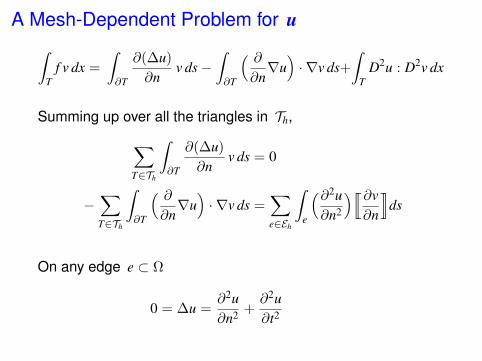
On any edge e ⊂ Ω
0 = ∆u
A Mesh-Dependent Problem for u∫T
f v dx =
∫∂T
∂(∆u)
∂nv ds−
∫∂T
( ∂∂n∇u)· ∇v ds+
∫T
D2u : D2v dx
Summing up over all the triangles in Th,∑T∈Th
∫∂T
∂(∆u)
∂nv ds = 0
−∑T∈Th
∫∂T
( ∂∂n∇u)· ∇v ds =
∑e∈Eh
∫e
(∂2u∂n2
)[[∂v∂n
]]ds
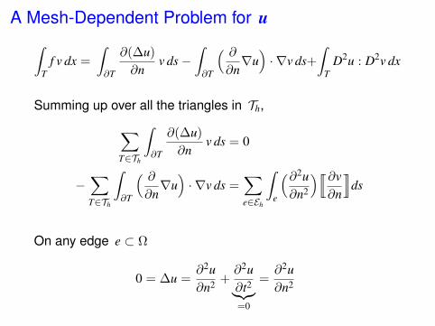
On any edge e ⊂ Ω
0 = ∆u =∂2u∂n2 +
∂2u∂t2
A Mesh-Dependent Problem for u∫T
f v dx =
∫∂T
∂(∆u)
∂nv ds−
∫∂T
( ∂∂n∇u)· ∇v ds+
∫T
D2u : D2v dx
Summing up over all the triangles in Th,∑T∈Th
∫∂T
∂(∆u)
∂nv ds = 0
−∑T∈Th
∫∂T
( ∂∂n∇u)· ∇v ds =
∑e∈Eh
∫e
(∂2u∂n2
)[[∂v∂n
]]ds
On any edge e ⊂ Ω
0 = ∆u =∂2u∂n2 +
∂2u∂t2︸︷︷︸=0
=∂2u∂n2
A Mesh-Dependent Problem for u∫T
f v dx =
∫∂T
∂(∆u)
∂nv ds−
∫∂T
( ∂∂n∇u)· ∇v ds+
∫T
D2u : D2v dx
Summing up over all the triangles in Th,∑T∈Th
∫∂T
∂(∆u)
∂nv ds = 0
−∑T∈Th
∫∂T
( ∂∂n∇u)· ∇v ds =
∑e∈Eh
∫e
(∂2u∂n2
)[[∂v∂n
]]ds
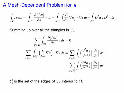
=∑e∈E i
h
∫e
(∂2u∂n2
)[[∂v∂n
]]ds
E ih is the set of the edges of Th interior to Ω.
A Mesh-Dependent Problem for u∫T
f v dx =
∫∂T
∂(∆u)
∂nv ds−
∫∂T
( ∂∂n∇u)· ∇v ds+
∫T
D2u : D2v dx
Summing up over all the triangles in Th,∑T∈Th
∫∂T
∂(∆u)
∂nv ds = 0
−∑T∈Th
∫∂T
( ∂∂n∇u)· ∇v ds =
∑e∈Eh
∫e
(∂2u∂n2
)[[∂v∂n
]]ds
=∑e∈E i
h
∫e
(∂2u∂n2
)[[∂v∂n
]]ds
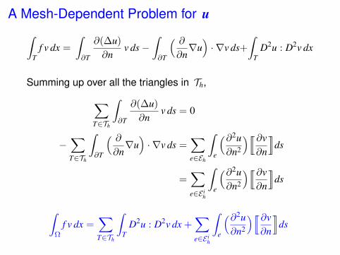
∫Ω
f v dx =∑T∈Th
∫T
D2u : D2v dx +∑e∈E i
h
∫e
(∂2u∂n2
)[[∂v∂n
]]ds
A Mesh-Dependent Problem for u
∫Ω
f v dx =∑T∈Th
∫T
D2u : D2v dx +∑e∈E i
h
∫e
(∂2u∂n2
)[[∂v∂n
]]ds
A Mesh-Dependent Problem for u
∫Ω
f v dx =∑T∈Th
∫T
D2u : D2v dx +∑e∈E i
h
∫e
(∂2u∂n2
)[[∂v∂n
]]ds
=∑T∈Th
∫T
D2u : D2v dx +∑e∈E i
h
∫e
∂2u∂n2
[[∂v∂n
]]ds
∂2u∂n2
=∂2u∂n2
A Mesh-Dependent Problem for u
∫Ω
f v dx =∑T∈Th
∫T
D2u : D2v dx +∑e∈E i
h
∫e
(∂2u∂n2
)[[∂v∂n
]]ds
=∑T∈Th
∫T
D2u : D2v dx +∑e∈E i
h
∫e
∂2u∂n2
[[∂v∂n
]]ds
+∑e∈E i
h
∫e
∂2v∂n2
[[∂u∂n
]]︸ ︷︷ ︸
=0
ds
symmetrization
A Mesh-Dependent Problem for u
∫Ω
f v dx =∑T∈Th
∫T
D2u : D2v dx +∑e∈E i
h
∫e
(∂2u∂n2
)[[∂v∂n
]]ds
=∑T∈Th
∫T
D2u : D2v dx +∑e∈E i
h
∫e
∂2u∂n2
[[∂v∂n
]]ds
+∑e∈E i
h
∫e
∂2v∂n2
[[∂u∂n
]]ds
+ σ∑e∈E i
h
1|e|
∫e
[[∂u∂n
]]︸ ︷︷ ︸
=0
[[∂v∂n
]]ds
stabilization
A Mesh-Dependent Problem for uThe solution u of the continuous problem satisfies
ah(u, v) =
∫Ω
f v dx ∀ v ∈ Vh
ah(w, v) =∑T∈Th
∫T
D2w : D2v dx +∑e∈E i
h
∫e
∂2w∂n2
[[∂v∂n
]]ds
+∑e∈E i
h
∫e
∂2v∂n2
[[∂w∂n
]]ds
+ σ∑e∈E i
h
1|e|
∫e
[[∂w∂n
]][[∂v∂n
]]ds
E ih = set of interior edges · = average [[·]] = jump
|e| = length of e σ = penalty parameter
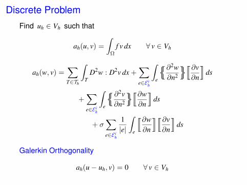
Discrete Problem
Find uh ∈ Vh such that
ah(u, v) =
∫Ω
f v dx ∀ v ∈ Vh
ah(w, v) =∑T∈Th
∫T
D2w : D2v dx +∑e∈E i
h
∫e
∂2w∂n2
[[∂v∂n
]]ds
+∑e∈E i
h
∫e
∂2v∂n2
[[∂w∂n
]]ds
+ σ∑e∈E i
h
1|e|
∫e
[[∂w∂n
]][[∂v∂n
]]ds
Galerkin Orthogonality
ah(u− uh, v) = 0 ∀ v ∈ Vh
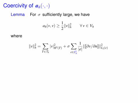
Coercivity of ah(·, ·)Lemma For σ sufficiently large, we have
ah(v, v) ≥ 12‖v‖2
h ∀ v ∈ Vh
where
‖v‖2h =
∑T∈Th
|v|2H2(T) + σ∑e∈E i
h
1|e|‖[[∂v/∂n]]‖2
L2(e)

Coercivity of ah(·, ·)Lemma For σ sufficiently large, we have
ah(v, v) ≥ 12‖v‖2
h ∀ v ∈ Vh
where
‖v‖2h =
∑T∈Th
|v|2H2(T) + σ∑e∈E i
h
1|e|‖[[∂v/∂n]]‖2
L2(e)
Consequently ah(·, ·) is SPD on Vh and hence the discreteproblem is well-posed.
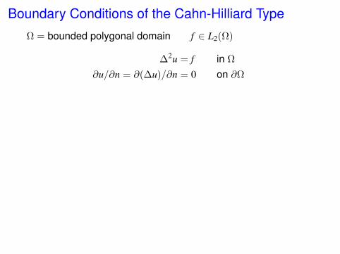
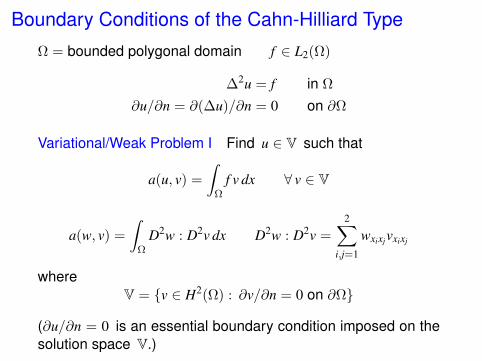
Boundary Conditions of the Cahn-Hilliard Type
Ω = bounded polygonal domain f ∈ L2(Ω)
∆2u = f in Ω
∂u/∂n = ∂(∆u)/∂n = 0 on ∂Ω
Boundary Conditions of the Cahn-Hilliard Type
Ω = bounded polygonal domain f ∈ L2(Ω)
∆2u = f in Ω
∂u/∂n = ∂(∆u)/∂n = 0 on ∂Ω
Variational/Weak Problem I Find u ∈ V such that
a(u, v) =
∫Ω
f v dx ∀ v ∈ V
a(w, v) =
∫Ω
D2w : D2v dx D2w : D2v =
2∑i,j=1
wxixjvxixj
whereV = v ∈ H2(Ω) : ∂v/∂n = 0 on ∂Ω
(∂u/∂n = 0 is an essential boundary condition imposed on thesolution space V.)
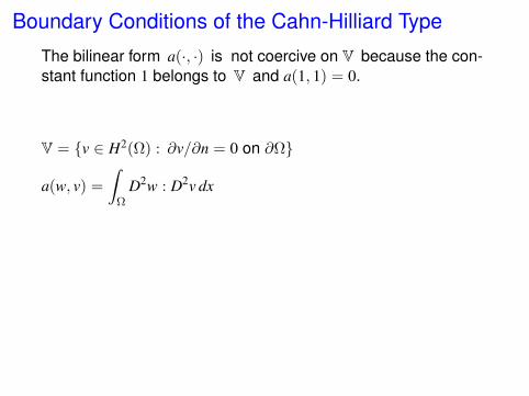
Boundary Conditions of the Cahn-Hilliard Type
The bilinear form a(·, ·) is not coercive on V because the con-stant function 1 belongs to V and a(1, 1) = 0.
V = v ∈ H2(Ω) : ∂v/∂n = 0 on ∂Ω
a(w, v) =
∫Ω
D2w : D2v dx
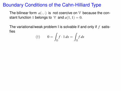
Boundary Conditions of the Cahn-Hilliard Type
The bilinear form a(·, ·) is not coercive on V because the con-stant function 1 belongs to V and a(1, 1) = 0.
The variational/weak problem I is solvable if and only if f satis-fies
(†) 0 =
∫Ω
f · 1 dx =
∫Ω
f dx

Boundary Conditions of the Cahn-Hilliard Type
The bilinear form a(·, ·) is not coercive on V because the con-stant function 1 belongs to V and a(1, 1) = 0.
The variational/weak problem I is solvable if and only if f satis-fies
(†) 0 =
∫Ω
f · 1 dx =
∫Ω
f dx
Under condition (†) the solution of the variational/weak problemI is unique up to an additive constant. In particular it has aunique solution in the subspace
V∗ = v ∈ V : v(p∗) = 0
where p∗ is a corner of Ω.
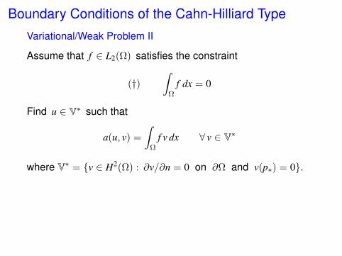
Boundary Conditions of the Cahn-Hilliard Type
Variational/Weak Problem II
Assume that f ∈ L2(Ω) satisfies the constraint
(†)∫
Ωf dx = 0
Find u ∈ V∗ such that
a(u, v) =
∫Ω
f v dx ∀ v ∈ V∗
where V∗ = v ∈ H2(Ω) : ∂v/∂n = 0 on ∂Ω and v(p∗) = 0.
Boundary Conditions of the Cahn-Hilliard Type
Variational/Weak Problem II
Assume that f ∈ L2(Ω) satisfies the constraint
(†)∫
Ωf dx = 0
Find u ∈ V∗ such that
a(u, v) =
∫Ω
f v dx ∀ v ∈ V∗
where V∗ = v ∈ H2(Ω) : ∂v/∂n = 0 on ∂Ω and v(p∗) = 0.
Since the bilinear form a(·, ·) is bounded and coercive on V∗,the variational/weak problem II has a unique solution, whichis also a solution of the variational/weak problem I due to thecondition (†).
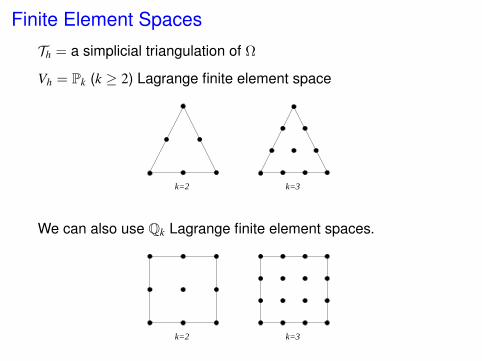
Finite Element Spaces
Th = a simplicial triangulation of Ω
Vh = Pk (k ≥ 2) Lagrange finite element space
k=3k=2
We can also use Qk Lagrange finite element spaces.
k=3k=2
Finite Element Spaces
Th = a simplicial triangulation of Ω
Vh = Pk (k ≥ 2) Lagrange finite element space
k=3k=2
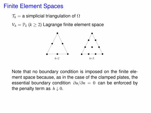
Note that no boundary condition is imposed on the finite ele-ment space because, as in the case of the clamped plates, theessential boundary condition ∂u/∂n = 0 can be enforced bythe penalty term as h ↓ 0.
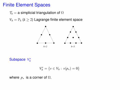
Finite Element Spaces
Th = a simplicial triangulation of Ω
Vh = Pk (k ≥ 2) Lagrange finite element space
k=3k=2
Subspace V∗h
V∗h = v ∈ Vh : v(p∗) = 0
where p∗ is a corner of Ω.

A Mesh-Dependent Problem for u
A Mesh-Dependent Problem for u∫T
f v dx =
∫∂T
∂(∆u)
∂nv ds−
∫∂T
( ∂∂n∇u)· ∇v ds+
∫T
D2u : D2v dx
A Mesh-Dependent Problem for u∫T
f v dx =
∫∂T
∂(∆u)
∂nv ds−
∫∂T
( ∂∂n∇u)· ∇v ds+
∫T
D2u : D2v dx
Summing up over all the triangles in Th,
∑T∈Th
∫∂T
∂(∆u)
∂nv ds = 0
Each interior edge is shared by two triangles. Since v and thederivatives of u are continuous and the normals from the twotriangles are pointing at opposite directions, the contributionsfrom the two triangles cancel.
There is also no contribution from the boundary edges because∂(∆u)/∂n = 0 on ∂Ω.
A Mesh-Dependent Problem for u∫T
f v dx =
∫∂T
∂(∆u)
∂nv ds−
∫∂T
( ∂∂n∇u)· ∇v ds+
∫T
D2u : D2v dx
Summing up over all the triangles in Th,
∑T∈Th
∫∂T
∂(∆u)
∂nv ds = 0
−∑T∈Th
∫∂T
( ∂∂n∇u)· ∇v ds =
∑e∈Eh
∫e
(∂2u∂n2
)[[∂v∂n
]]ds
[[∂v/∂t]] = 0 over interior edges.
∂
∂t
(∂u∂n
)= 0 on boundary edges.
A Mesh-Dependent Problem for u∫T
f v dx =
∫∂T
∂(∆u)
∂nv ds−
∫∂T
( ∂∂n∇u)· ∇v ds+
∫T
D2u : D2v dx
Summing up over all the triangles in Th,
∑T∈Th
∫∂T
∂(∆u)
∂nv ds = 0
−∑T∈Th
∫∂T
( ∂∂n∇u)· ∇v ds =
∑e∈Eh
∫e
(∂2u∂n2
)[[∂v∂n
]]ds
∫Ω
f v dx =∑T∈Th
∫T
D2u : D2v dx +∑e∈Eh
∫e
(∂2u∂n2
)[[∂v∂n
]]ds

A Mesh-Dependent Problem for uThe solution u of the continuous problem satisfies
ah(u, v) =
∫Ω
f v dx ∀ v ∈ Vh
ah(w, v) =∑T∈Th
∫T
D2w : D2v dx +∑e∈Eh
∫e
∂2w∂n2
[[∂v∂n
]]ds
+∑e∈Eh
∫e
∂2v∂n2
[[∂w∂n
]]ds
+ σ∑e∈Eh
1|e|
∫e
[[∂w∂n
]][[∂v∂n
]]ds
Eh = set of edges · = average [[·]] = jump
|e| = length of e σ = penalty parameter

Discrete Problem
Find uh ∈ V∗h such that (V∗h = v ∈ Vh : v(p∗) = 0)
ah(uh, v) =
∫Ω
f v dx ∀ v ∈ V∗h
ah(w, v) =∑T∈Th
∫T
D2w : D2v dx +∑e∈Eh
∫e
∂2w∂n2
[[∂v∂n
]]ds
+∑e∈Eh
∫e
∂2v∂n2
[[∂w∂n
]]ds
+ σ∑e∈Eh
1|e|
∫e
[[∂w∂n
]][[∂v∂n
]]ds
Galerkin Orthogonality
ah(u− uh, v) = 0 ∀ v ∈ V∗h
Coercivity of ah(·, ·)Lemma For σ sufficiently large, we have
ah(v, v) ≥ 12‖v‖2
h ∀ v ∈ V∗h
where
‖v‖2h =
∑T∈Th
|v|2H2(T) + σ∑e∈Eh
1|e|‖[[∂v/∂n]]‖2
L2(e)
Consequently ah(·, ·) is SPD on V∗h and hence the discreteproblem is well-posed.
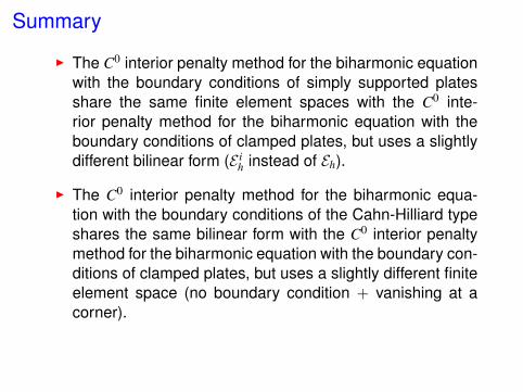
Summary
I The C0 interior penalty method for the biharmonic equationwith the boundary conditions of simply supported platesshare the same finite element spaces with the C0 inte-rior penalty method for the biharmonic equation with theboundary conditions of clamped plates, but uses a slightlydifferent bilinear form (E i
h instead of Eh).
I The C0 interior penalty method for the biharmonic equa-tion with the boundary conditions of the Cahn-Hilliard typeshares the same bilinear form with the C0 interior penaltymethod for the biharmonic equation with the boundary con-ditions of clamped plates, but uses a slightly different finiteelement space (no boundary condition + vanishing at acorner).
Enriching Operators
Enriching Operators
Enriching Operators
Clamped Plates
Solution space for the continuous problem is H20(Ω).
Solution space for the discrete problem is a Pk (or Qk) Lagrangefinite element space Vh ⊂ H1
0(Ω).
Enriching Operators
Clamped Plates
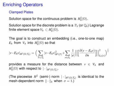
Solution space for the continuous problem is H20(Ω).
Solution space for the discrete problem is a Pk (or Qk) Lagrangefinite element space Vh ⊂ H1
0(Ω).
The goal is to construct an embedding (i.e., one-to-one map)Eh from Vh into H2
0(Ω) so that
|v−Ehv|H2(Ω;Th) =( ∑
T∈Th
|v−Ehv|2H2(T)+∑e∈Eh
1|e|
∥∥∥[[∂(v− Ehv)
∂n
]]∥∥∥2
L2(e)
) 12
provides a measure for the distance between v ∈ Vh andH2
0(Ω) with respect to | · |H2(Ω;Th).
(The piecewise H2 (semi-) norm | · |H2(Ω;Th) is identical to themesh-dependent norm ‖ · ‖h when σ = 1.)

C1 Relatives
C1 Relatives
We say that a C1 element is a (rich) relative of a Lagrangeelement if
they have the same element domain,
the shape functions of the Lagrange finite element are alsoshape functions for the C1 element,
the dofs for the Lagrange element are also dofs for the C1
element.

C1 Relatives
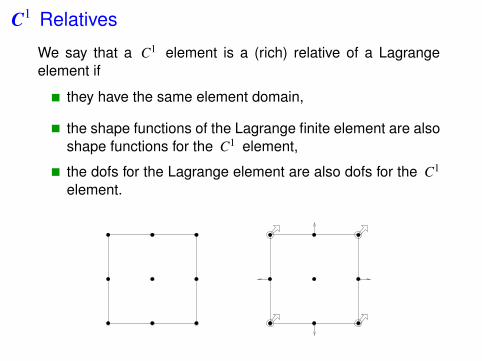
We say that a C1 element is a (rich) relative of a Lagrangeelement if
they have the same element domain,
the shape functions of the Lagrange finite element are alsoshape functions for the C1 element,
the dofs for the Lagrange element are also dofs for the C1
element.
C1 Relatives
We say that a C1 element is a (rich) relative of a Lagrangeelement if
they have the same element domain,
the shape functions of the Lagrange finite element are alsoshape functions for the C1 element,
the dofs for the Lagrange element are also dofs for the C1
element.

Averaging
Averaging
Vh = Q2 Lagrange Finite Element Space
Eh : Vh −→ Wh ⊂ H20(Ω)
where Wh is the Q4 BFS finite element space.
Averaging
Vh = Q2 Lagrange Finite Element Space
Eh : Vh −→ Wh ⊂ H20(Ω)
where Wh is the Q4 BFS finite element space.
Let v ∈ Vh. Since the dofs of Ehv along the boundary of Ωmust vanish by the condition that Ehv ∈ H2
0(Ω), we only need tospecify the dofs at the nodes interior to Ω.
Averaging
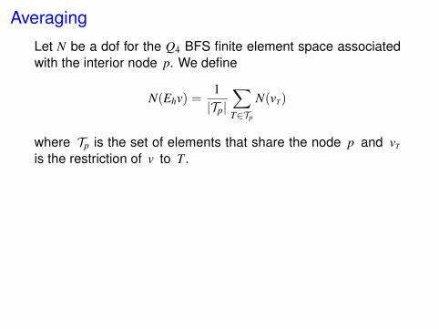
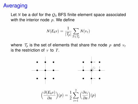
Let N be a dof for the Q4 BFS finite element space associatedwith the interior node p. We define
N(Ehv) =1|Tp|
∑T∈Tp
N(vT)
where Tp is the set of elements that share the node p and vT
is the restriction of v to T.
Averaging
Let N be a dof for the Q4 BFS finite element space associatedwith the interior node p. We define
N(Ehv) =1|Tp|
∑T∈Tp
N(vT)
where Tp is the set of elements that share the node p and vT
is the restriction of v to T.
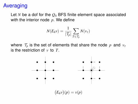
(Ehv)(p) = v(p)

Averaging
Let N be a dof for the Q4 BFS finite element space associatedwith the interior node p. We define
N(Ehv) =1|Tp|
∑T∈Tp
N(vT)
where Tp is the set of elements that share the node p and vT
is the restriction of v to T.
(∇(Ehv)
)(p) =
14
4∑i=1
(∇vi)(p)
Averaging
Let N be a dof for the Q4 BFS finite element space associatedwith the interior node p. We define
N(Ehv) =1|Tp|
∑T∈Tp
N(vT)
where Tp is the set of elements that share the node p and vT
is the restriction of v to T.
(∂(Ehv)
∂n
)(p) =
12
2∑i=1
(∂vi
∂n
)(p)
Averaging
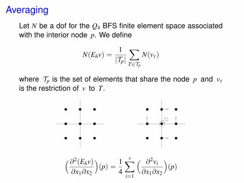
Let N be a dof for the Q4 BFS finite element space associatedwith the interior node p. We define
N(Ehv) =1|Tp|
∑T∈Tp
N(vT)
where Tp is the set of elements that share the node p and vT
is the restriction of v to T.
(∂2(Ehv)
∂x1∂x2
)(p) =
14
4∑i=1
( ∂2vi
∂x1∂x2
)(p)
Properties of Eh
Properties of Eh
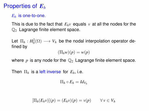
Eh is one-to-one.
This is due to the fact that Ehv equals v at all the nodes for theQ2 Lagrange finite element space.
Properties of Eh
Eh is one-to-one.
This is due to the fact that Ehv equals v at all the nodes for theQ2 Lagrange finite element space.
Let Πh : H20(Ω) −→ Vh be the nodal interpolation operator de-
fined by(Πhw)(p) = w(p)
where p is any node for the Q2 Lagrange finite element space.
Then Πh is a left inverse for Eh, i.e.
Πh Eh = IdVh
[Πh(Ehv)](p) = (Ehv)(p) = v(p) ∀ v ∈ Vh
Properties of Eh
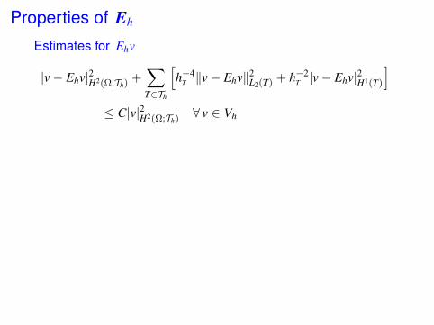
Estimates for Ehv
|v− Ehv|2H2(Ω;Th) +∑T∈Th
[h−4
T ‖v− Ehv‖2L2(T) + h−2
T |v− Ehv|2H1(T)
]≤ C|v|2H2(Ω;Th) ∀ v ∈ Vh
Properties of Eh
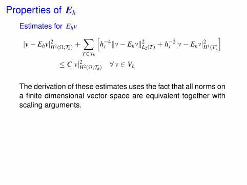
Estimates for Ehv
|v− Ehv|2H2(Ω;Th) +∑T∈Th
[h−4
T ‖v− Ehv‖2L2(T) + h−2
T |v− Ehv|2H1(T)
]≤ C|v|2H2(Ω;Th) ∀ v ∈ Vh
The derivation of these estimates uses the fact that all norms ona finite dimensional vector space are equivalent together withscaling arguments.

Properties of Eh
Estimates for Ehv
|v− Ehv|2H2(Ω;Th) +∑T∈Th
[h−4
T ‖v− Ehv‖2L2(T) + h−2
T |v− Ehv|2H1(T)
]≤ C|v|2H2(Ω;Th) ∀ v ∈ Vh
The derivation of these estimates uses the fact that all norms ona finite dimensional vector space are equivalent together withscaling arguments.
Corollary
|Ehv|H2(Ω) = |Ehv|H2(Ω;Th)
≤ |Ehv− v|H2(Ω;Th) + |v|H2(Ω;Th)
≤ C|v|H2(Ω;Th) ∀ v ∈ Vh
Properties of Eh
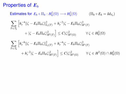
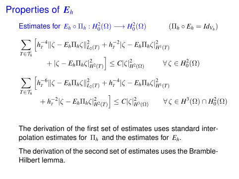
Estimates for Eh Πh : H20(Ω) −→ H2
0(Ω) (Πh Eh = IdVh)∑T∈Th
[h−4
T ‖ζ − EhΠhζ‖2L2(T) + h−2
T |ζ − EhΠhζ|2H1(T)
+ |ζ − EhΠhζ|2H2(T)
]≤ C|ζ|2H2(Ω) ∀ ζ ∈ H2
0(Ω)∑T∈Th
[h−6
T ‖ζ − EhΠhζ‖2L2(T) + h−4
T |ζ − EhΠhζ|2H1(T)
+ h−2T |ζ − EhΠhζ|2H2(T)
]≤ C|ζ|2H3(Ω) ∀ ζ ∈ H3(Ω) ∩ H2
0(Ω)
Properties of Eh
Estimates for Eh Πh : H20(Ω) −→ H2
0(Ω) (Πh Eh = IdVh)∑T∈Th
[h−4
T ‖ζ − EhΠhζ‖2L2(T) + h−2
T |ζ − EhΠhζ|2H1(T)
+ |ζ − EhΠhζ|2H2(T)
]≤ C|ζ|2H2(Ω) ∀ ζ ∈ H2
0(Ω)∑T∈Th
[h−6
T ‖ζ − EhΠhζ‖2L2(T) + h−4
T |ζ − EhΠhζ|2H1(T)
+ h−2T |ζ − EhΠhζ|2H2(T)
]≤ C|ζ|2H3(Ω) ∀ ζ ∈ H3(Ω) ∩ H2
0(Ω)
The derivation of the first set of estimates uses standard inter-polation estimates for Πh and the estimates for Eh.
The derivation of the second set of estimates uses the Bramble-Hilbert lemma.

Properties of Eh
Estimates for Eh Πh : H20(Ω) −→ H2
0(Ω) (Πh Eh = IdVh)∑T∈Th
[h−4
T ‖ζ − EhΠhζ‖2L2(T) + h−2
T |ζ − EhΠhζ|2H1(T)
+ |ζ − EhΠhζ|2H2(T)
]≤ C|ζ|2H2(Ω) ∀ ζ ∈ H2
0(Ω)∑T∈Th
[h−6
T ‖ζ − EhΠhζ‖2L2(T) + h−4
T |ζ − EhΠhζ|2H1(T)
+ h−2T |ζ − EhΠhζ|2H2(T)
]≤ C|ζ|2H3(Ω) ∀ ζ ∈ H3(Ω) ∩ H2
0(Ω)
These estimates indicate that Eh Πh is a quasi-local interpo-lation operator from H2
0(Ω) into a C1 finite element space thatsatisfies the correct discretization error estimates.
Properties of Eh
Estimates for Eh Πh : H20(Ω) −→ H2
0(Ω) (Πh Eh = IdVh)∑T∈Th
[h−4
T ‖ζ − EhΠhζ‖2L2(T) + h−2
T |ζ − EhΠhζ|2H1(T)
+ |ζ − EhΠhζ|2H2(T)
]≤ C|ζ|2H2(Ω) ∀ ζ ∈ H2
0(Ω)∑T∈Th
[h−6
T ‖ζ − EhΠhζ‖2L2(T) + h−4
T |ζ − EhΠhζ|2H1(T)
+ h−2T |ζ − EhΠhζ|2H2(T)
]≤ C|ζ|2H3(Ω) ∀ ζ ∈ H3(Ω) ∩ H2
0(Ω)
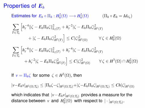
If v = Πhζ for some ζ ∈ H3(Ω), then
|v−Ehv|H2(Ω;Th) ≤ |Πhζ−ζ|H2(Ω;Th)+|ζ−EhΠhζ|H2(Ω;Th) ≤ Ch|ζ|H3(Ω)
which indicates that |v−Ehv|H2(Ω;Th) provides a measure for thedistance between v and H2
0(Ω) with respect to | · |H2(Ω;Th).

Other Boundary Conditions
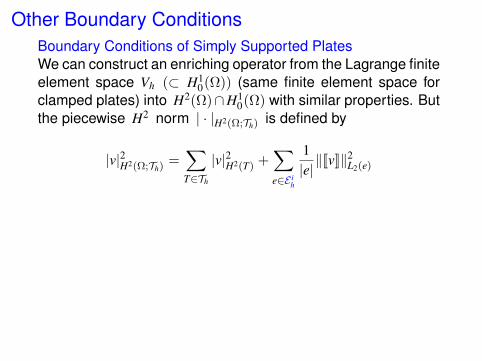
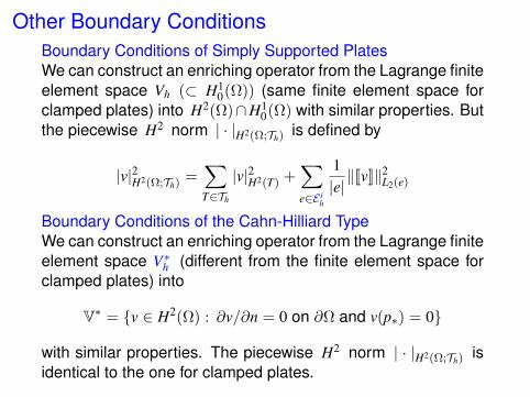
Other Boundary ConditionsBoundary Conditions of Simply Supported PlatesWe can construct an enriching operator from the Lagrange finiteelement space Vh (⊂ H1
0(Ω)) (same finite element space forclamped plates) into H2(Ω)∩H1
0(Ω) with similar properties. Butthe piecewise H2 norm | · |H2(Ω;Th) is defined by
|v|2H2(Ω;Th) =∑T∈Th
|v|2H2(T) +∑e∈E i
h
1|e|‖[[v]]‖2
L2(e)
Boundary Conditions of the Cahn-Hilliard TypeWe can construct an enriching operator from the Lagrange finiteelement space V∗h (different from the finite element space forclamped plates) into
V∗ = v ∈ H2(Ω) : ∂v/∂n = 0 on ∂Ω and v(p∗) = 0
with similar properties. The piecewise H2 norm | · |H2(Ω;Th) isidentical to the one for clamped plates.
Post-Processing by Eh
Post-Processing by Eh
Let uh ∈ Vh be the solution of a C0 interior penalty methodfor the biharmonic equation with the boundary condition of theclamped plates (respectively simply supported plates or Cahn-Hilliard type) and Eh be an enriching operator from Eh intoH2
0(Ω) (respectively H2(Ω) ∩ H10(Ω) or V∗).
Then Ehuh is a conforming approximation of the boundaryvalue problem obtained from uh by post-processing.
It can be shown, by using the error estimates of the C0 interiorpenalty methods (to be discussed) and properties of Eh, thatEhuh is a C1 approximate solution with correct estimates.
Therefore C0 interior penalty methods are relevant even if weonly want C1 approximate solutions.
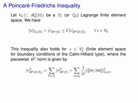
A Poincaré-Friedrichs Inequality
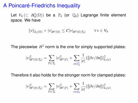
Let Vh (⊂ H10(Ω)) be a Pk (or Qk) Lagrange finite element
space. We have
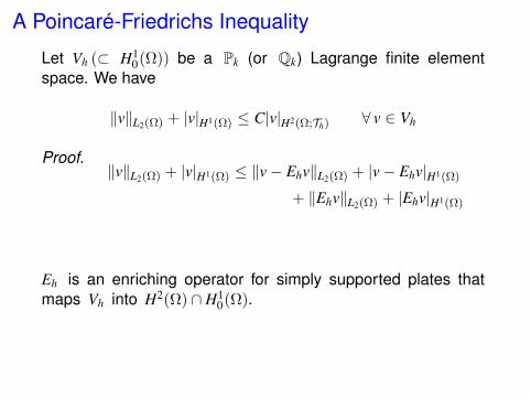
‖v‖L2(Ω) + |v|H1(Ω) ≤ C|v|H2(Ω;Th) ∀ v ∈ Vh
A Poincaré-Friedrichs Inequality
Let Vh (⊂ H10(Ω)) be a Pk (or Qk) Lagrange finite element
space. We have
‖v‖L2(Ω) + |v|H1(Ω) ≤ C|v|H2(Ω;Th) ∀ v ∈ Vh
The piecewise H2 norm is the one for simply supported plates:
|v|2H2(Ω;Th) =∑T∈Th
|v|2H2(T) +∑e∈E i
h
1|e|‖[[∂v/∂n]]‖2
L2(e)
Therefore it also holds for the stronger norm for clamped plates:
|v|2H2(Ω;Th) =∑T∈Th
|v|2H2(T) +∑e∈Eh
1|e|‖[[∂v/∂n]]‖2
L2(e)
A Poincaré-Friedrichs Inequality
Let Vh (⊂ H10(Ω)) be a Pk (or Qk) Lagrange finite element
space. We have
‖v‖L2(Ω) + |v|H1(Ω) ≤ C|v|H2(Ω;Th) ∀ v ∈ Vh
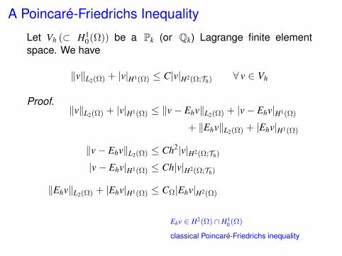
Proof.‖v‖L2(Ω) + |v|H1(Ω) ≤ ‖v− Ehv‖L2(Ω) + |v− Ehv|H1(Ω)
+ ‖Ehv‖L2(Ω) + |Ehv|H1(Ω)
Eh is an enriching operator for simply supported plates thatmaps Vh into H2(Ω) ∩ H1
0(Ω).

A Poincaré-Friedrichs Inequality
Let Vh (⊂ H10(Ω)) be a Pk (or Qk) Lagrange finite element
space. We have
‖v‖L2(Ω) + |v|H1(Ω) ≤ C|v|H2(Ω;Th) ∀ v ∈ Vh
Proof.‖v‖L2(Ω) + |v|H1(Ω) ≤ ‖v− Ehv‖L2(Ω) + |v− Ehv|H1(Ω)
+ ‖Ehv‖L2(Ω) + |Ehv|H1(Ω)
‖v− Ehv‖L2(Ω) ≤ Ch2|v|H2(Ω;Th)
|v− Ehv|H1(Ω) ≤ Ch|v|H2(Ω;Th)
∑T∈Th
[h−4
T ‖v− Ehv‖2L2(T) + h−2
T |v− Ehv|2H1(T)
]≤ C|v|2H2(Ω;Th)
A Poincaré-Friedrichs Inequality
Let Vh (⊂ H10(Ω)) be a Pk (or Qk) Lagrange finite element
space. We have
‖v‖L2(Ω) + |v|H1(Ω) ≤ C|v|H2(Ω;Th) ∀ v ∈ Vh
Proof.‖v‖L2(Ω) + |v|H1(Ω) ≤ ‖v− Ehv‖L2(Ω) + |v− Ehv|H1(Ω)
+ ‖Ehv‖L2(Ω) + |Ehv|H1(Ω)
‖v− Ehv‖L2(Ω) ≤ Ch2|v|H2(Ω;Th)
|v− Ehv|H1(Ω) ≤ Ch|v|H2(Ω;Th)
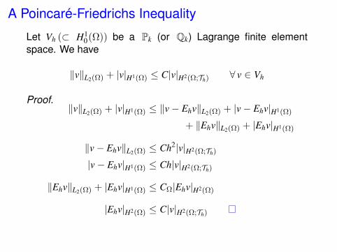
‖Ehv‖L2(Ω) + |Ehv|H1(Ω) ≤ CΩ|Ehv|H2(Ω)
Ehv ∈ H2(Ω) ∩ H10(Ω)
classical Poincaré-Friedrichs inequality
A Poincaré-Friedrichs Inequality
Let Vh (⊂ H10(Ω)) be a Pk (or Qk) Lagrange finite element
space. We have
‖v‖L2(Ω) + |v|H1(Ω) ≤ C|v|H2(Ω;Th) ∀ v ∈ Vh
Proof.‖v‖L2(Ω) + |v|H1(Ω) ≤ ‖v− Ehv‖L2(Ω) + |v− Ehv|H1(Ω)
+ ‖Ehv‖L2(Ω) + |Ehv|H1(Ω)
‖v− Ehv‖L2(Ω) ≤ Ch2|v|H2(Ω;Th)
|v− Ehv|H1(Ω) ≤ Ch|v|H2(Ω;Th)
‖Ehv‖L2(Ω) + |Ehv|H1(Ω) ≤ CΩ|Ehv|H2(Ω)
|Ehv|H2(Ω) ≤ C|v|H2(Ω;Th)
A Poincaré-Friedrichs Inequality
Let Vh (⊂ H10(Ω)) be a Pk (or Qk) Lagrange finite element
space. We have
‖v‖L2(Ω) + |v|H1(Ω) ≤ C|v|H2(Ω;Th) ∀ v ∈ Vh
This inequality also holds for v ∈ V∗h (finite element spacefor boundary conditions of the Cahn-Hilliard type), where thepiecewise H2 norm is given by
|v|2H2(Ω;Th) =∑T∈Th
|v|2H2(T) +∑e∈Eh
1|e|‖[[∂v/∂n]]‖2
L2(e)

An Application of the Poincaré-Friedrichs Inequality
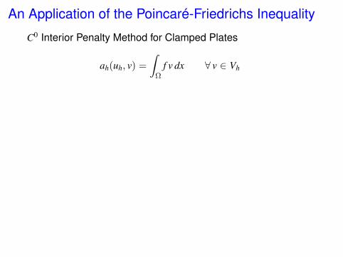
An Application of the Poincaré-Friedrichs Inequality
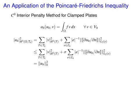
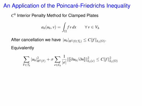
C0 Interior Penalty Method for Clamped Plates
ah(uh, v) =
∫Ω
f v dx ∀ v ∈ Vh
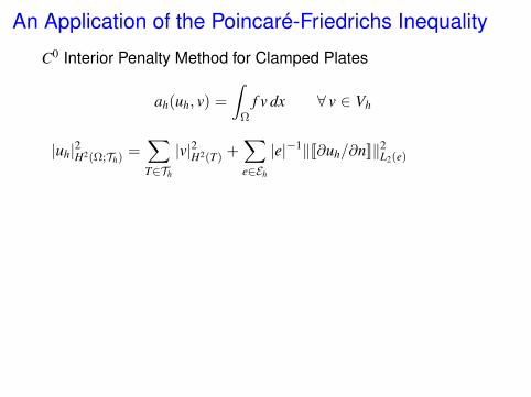
An Application of the Poincaré-Friedrichs Inequality
C0 Interior Penalty Method for Clamped Plates
ah(uh, v) =
∫Ω
f v dx ∀ v ∈ Vh
|uh|2H2(Ω;Th) =∑T∈Th
|v|2H2(T) +∑e∈Eh
|e|−1‖[[∂uh/∂n]]‖2L2(e)
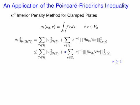
An Application of the Poincaré-Friedrichs Inequality
C0 Interior Penalty Method for Clamped Plates
ah(uh, v) =
∫Ω
f v dx ∀ v ∈ Vh
|uh|2H2(Ω;Th) =∑T∈Th
|v|2H2(T) +∑e∈Eh
|e|−1‖[[∂uh/∂n]]‖2L2(e)
≤∑T∈Th
|v|2H2(T) + σ∑e∈Eh
|e|−1‖[[∂uh/∂n]]‖2L2(e)
σ ≥ 1
An Application of the Poincaré-Friedrichs Inequality
C0 Interior Penalty Method for Clamped Plates
ah(uh, v) =
∫Ω
f v dx ∀ v ∈ Vh
|uh|2H2(Ω;Th) =∑T∈Th
|v|2H2(T) +∑e∈Eh
|e|−1‖[[∂uh/∂n]]‖2L2(e)
≤∑T∈Th
|v|2H2(T) + σ∑e∈Eh
|e|−1‖[[∂uh/∂n]]‖2L2(e)
= ‖uh‖2h
An Application of the Poincaré-Friedrichs Inequality
C0 Interior Penalty Method for Clamped Plates
ah(uh, v) =
∫Ω
f v dx ∀ v ∈ Vh
|uh|2H2(Ω;Th) =∑T∈Th
|v|2H2(T) +∑e∈Eh
|e|−1‖[[∂uh/∂n]]‖2L2(e)
≤∑T∈Th
|v|2H2(T) + σ∑e∈Eh
|e|−1‖[[∂uh/∂n]]‖2L2(e)
= ‖uh‖2h
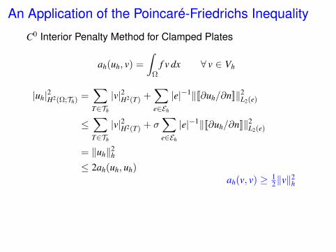
≤ 2ah(uh, uh)ah(v, v) ≥ 1
2‖v‖2h
An Application of the Poincaré-Friedrichs Inequality
C0 Interior Penalty Method for Clamped Plates
ah(uh, v) =
∫Ω
f v dx ∀ v ∈ Vh
|uh|2H2(Ω;Th) =∑T∈Th
|v|2H2(T) +∑e∈Eh
|e|−1‖[[∂uh/∂n]]‖2L2(e)
≤∑T∈Th
|v|2H2(T) + σ∑e∈Eh
|e|−1‖[[∂uh/∂n]]‖2L2(e)
= ‖uh‖2h
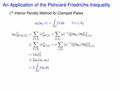
≤ 2ah(uh, uh)
= 2∫
Ωf uh dx

An Application of the Poincaré-Friedrichs Inequality
C0 Interior Penalty Method for Clamped Plates
ah(uh, v) =
∫Ω
f v dx ∀ v ∈ Vh
|uh|2H2(Ω;Th) =∑T∈Th
|v|2H2(T) +∑e∈Eh
|e|−1‖[[∂uh/∂n]]‖2L2(e)
≤∑T∈Th
|v|2H2(T) + σ∑e∈Eh
|e|−1‖[[∂uh/∂n]]‖2L2(e)
= ‖uh‖2h
≤ 2ah(uh, uh)
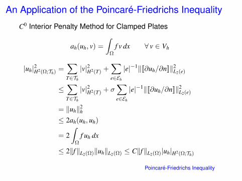
= 2∫
Ωf uh dx
≤ 2‖f‖L2(Ω)‖uh‖L2(Ω)
An Application of the Poincaré-Friedrichs Inequality
C0 Interior Penalty Method for Clamped Plates
ah(uh, v) =
∫Ω
f v dx ∀ v ∈ Vh
|uh|2H2(Ω;Th) =∑T∈Th
|v|2H2(T) +∑e∈Eh
|e|−1‖[[∂uh/∂n]]‖2L2(e)
≤∑T∈Th
|v|2H2(T) + σ∑e∈Eh
|e|−1‖[[∂uh/∂n]]‖2L2(e)
= ‖uh‖2h
≤ 2ah(uh, uh)
= 2∫
Ωf uh dx
≤ 2‖f‖L2(Ω)‖uh‖L2(Ω) ≤ C‖f‖L2(Ω)|uh|H2(Ω;Th)
Poincaré-Friedrichs Inequality
An Application of the Poincaré-Friedrichs Inequality
C0 Interior Penalty Method for Clamped Plates
ah(uh, v) =
∫Ω
f v dx ∀ v ∈ Vh
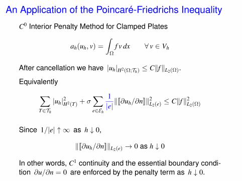
After cancellation we have |uh|H2(Ω;Th) ≤ C‖f‖L2(Ω).
Equivalently∑T∈Th
|uh|2H2(T) + σ∑e∈Eh
1|e|‖[[∂uh/∂n]]‖2
L2(e) ≤ C‖f‖2L2(Ω)
An Application of the Poincaré-Friedrichs Inequality
C0 Interior Penalty Method for Clamped Plates
ah(uh, v) =
∫Ω
f v dx ∀ v ∈ Vh
After cancellation we have |uh|H2(Ω;Th) ≤ C‖f‖L2(Ω).
Equivalently∑T∈Th
|uh|2H2(T) + σ∑e∈Eh
1|e|‖[[∂uh/∂n]]‖2
L2(e) ≤ C‖f‖2L2(Ω)
Since 1/|e| ↑ ∞ as h ↓ 0,
‖[[∂uh/∂n]]‖L2(e) → 0 as h ↓ 0
In other words, C1 continuity and the essential boundary condi-tion ∂u/∂n = 0 are enforced by the penalty term as h ↓ 0.
Reference
• B., K. Wang and J. Zhao
Poincaré-Friedrichs inequalities for piecewise H2 functions
Numer. Funct. Anal. Optim., 2004

Extensions
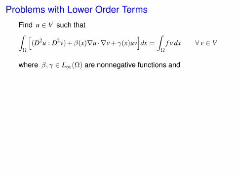
Problems with Lower Order Terms
Find u ∈ V such that∫Ω
[(D2u : D2v) +β(x)∇u ·∇v +γ(x)uv
]dx =
∫Ω
f v dx ∀ v ∈ V
where β, γ ∈ L∞(Ω) are nonnegative functions and
Problems with Lower Order Terms
Find u ∈ V such that∫Ω
[(D2u : D2v) +β(x)∇u ·∇v +γ(x)uv
]dx =
∫Ω
f v dx ∀ v ∈ V
where β, γ ∈ L∞(Ω) are nonnegative functions and
V = H20(Ω) for the boundary conditions of clamped plates,
Problems with Lower Order Terms
Find u ∈ V such that∫Ω
[(D2u : D2v) +β(x)∇u ·∇v +γ(x)uv
]dx =
∫Ω
f v dx ∀ v ∈ V
where β, γ ∈ L∞(Ω) are nonnegative functions and
V = H20(Ω) for the boundary conditions of clamped plates,
V = H2(Ω) ∩ H10(Ω) for the boundary conditions of simply
supported plates,

Problems with Lower Order Terms
Find u ∈ V such that∫Ω
[(D2u : D2v) +β(x)∇u ·∇v +γ(x)uv
]dx =
∫Ω
f v dx ∀ v ∈ V
where β, γ ∈ L∞(Ω) are nonnegative functions and
V = H20(Ω) for the boundary conditions of clamped plates,
V = H2(Ω) ∩ H10(Ω) for the boundary conditions of simply
supported plates,
V = V if γ 6= 0 and V = V∗ if γ = 0 (and∫
Ωf dx = 0) for
the boundary conditions of the Cahn-Hilliard type.
V = v ∈ H2(Ω) : ∂v/∂n = 0 on ∂ΩV∗ = v ∈ H2(Ω) : ∂v/∂n = 0 on ∂Ω and v(p∗) = 0

Problems with Lower Order Terms
Find u ∈ V such that∫Ω
[(D2u : D2v) +β(x)∇u ·∇v +γ(x)uv
]dx =
∫Ω
f v dx ∀ v ∈ V
where β, γ ∈ L∞(Ω) are nonnegative functions and
Modifications
Include ∫Ω
[β(x)∇w · ∇v + γ(x)wv
]dx
in the definition of the bilinear form ah(w, v).
Problems with Lower Order Terms
Find u ∈ V such that∫Ω
[(D2u : D2v) +β(x)∇u ·∇v +γ(x)uv
]dx =
∫Ω
f v dx ∀ v ∈ V
where β, γ ∈ L∞(Ω) are nonnegative functions and
Modifications
Include ∫Ω
[β(x)∇w · ∇v + γ(x)wv
]dx
in the definition of the bilinear form ah(w, v).
For boundary conditions of the Cahn-Hilliard type, removethe condition v(p∗) = 0 in the definition of the finite elementspace if γ 6= 0.

Problems with Less Regular Data
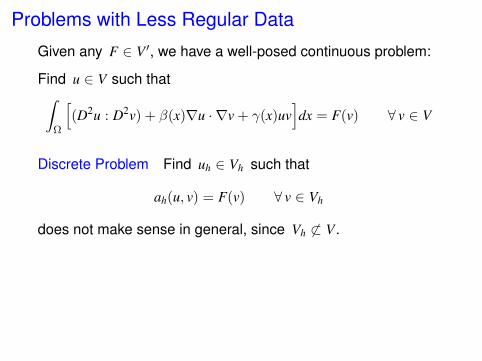
Problems with Less Regular Data
Given any F ∈ V ′, we have a well-posed continuous problem:
Find u ∈ V such that∫Ω
[(D2u : D2v) + β(x)∇u · ∇v + γ(x)uv
]dx = F(v) ∀ v ∈ V
Problems with Less Regular Data
Given any F ∈ V ′, we have a well-posed continuous problem:
Find u ∈ V such that∫Ω
[(D2u : D2v) + β(x)∇u · ∇v + γ(x)uv
]dx = F(v) ∀ v ∈ V
Discrete Problem Find uh ∈ Vh such that
ah(u, v) = F(v) ∀ v ∈ Vh
does not make sense in general, since Vh 6⊂ V.

Problems with Less Regular Data
Given any F ∈ V ′, we have a well-posed continuous problem:
Find u ∈ V such that∫Ω
[(D2u : D2v) + β(x)∇u · ∇v + γ(x)uv
]dx = F(v) ∀ v ∈ V
Discrete Problem Find uh ∈ Vh such that
ah(u, v) = F(v) ∀ v ∈ Vh
does not make sense in general, since Vh 6⊂ V.
Modification Find uh ∈ Vh such that
ah(u, v) = F(Ehv) ∀ v ∈ Vh
where Eh is the enriching operator from Vh into V.
Problems on Smooth Domains
We can also combine the C0 interior penalty approach with theisoparametric approach to solve fourth order boundary valueproblems on smooth domains.
Reference
• B., M. Neilan and L.-Y. Sung
Isoparametric C0 interior penalty methods
Calcolo, 2013
Other C0 Interior Penalty Methods
• G.N. Wells and N.T. Dung
A C0 discontinuous Galerkin formulation for Kirchhoffplates
Methods Appl. Mech. Engrg., 2007
• J. Huang, X. Huang and W. Han
A new C0 discontinuous Galerkin method for Kirchhoffplates,
Methods Appl. Mech. Engrg., 2010
• T. Gudi, H.S. Gupta and N. Nataraj
Analysis of an interior penalty method for fourth order prob-lems on polygonal domains
J. Sci. Comp., 2013


