Classroom Tips and Techniques: Mathematical Thoughts on the Root Locus

Robert J. LopezEmeritus Professor of Mathematics and Maple Fellow

Maplesoft

Introduction

Under mild continuity requirements, the equation , an equation in with real parameter , will have roots that trace a trajectory in the -plane when is real, and a different trajectoryin the complex -plane when is complex. In either event, such trajectories might be thought of as the loci of roots.

In the particular application where is the characteristic polynomial for a closed-loop feedback-control system, the trajectory in the complex plane is called a root locus. In the language of engineering control theory [1], "...the root locus is the locus of values of for which is satisfied as the real parameter varies from zero to infinity." The real parameter , called a "gain,"typically controls the amount of "feedback" in the control system, and is the transfer function for the open-loop control system. Of course, the transfer function arises from the Laplace transform of the differential equation governing the system.

Regardless of the origins of the need for a root locus, the notion of a trajectory hidden in the parameter-dependent roots of an equation is interesting in its own right. Hence, this article explores the phenomenon of the locus of roots, both as an object of practical use for the controls engineer and as an object of speculation and abstract thought for the mathematician.

Example 1

How do the zeros of depend on the parameter ?

Solution

An explicit solution for the zeros is immediate upon applying the quadratic formula to the equation .

0

Figure 1 contains the locus of for real. For , is complex; hence the gap between the branches in Figure 1. Figure 2 contains the locus of drawn in the complex plane. When is real, the locus lies along the real axis. When is complex, the locus departs

from the real axis and traverses through the upper and lower halves of the complex plane. A controls engineer could call Figure 2 a "root locus."

Figure 1 The zeros drawn in the real -plane

Figure 2 The zeros drawn in the complex plane

Figure 3, an animation, provides a simultaneous tracing of the locus of roots in both the real and complex planes. The code for the animation is behind the button labeled "Figure 3".

Figure 3 Simultaneous animation of in the real and complex planes

Example 2

Obtain the root locus for the feedback system in which is the characteristic equation.

Note that the open-loop transfer function for which is

the closed-loop transfer function, corresponds to the transfer function for the differential equation .

Solution

The controls engineer is interested in the zeros of the characteristic polynomial, namely, the denominator of the closed-loop transfer function. Once again, these zeros are readily found with the quadratic formula.

0

Figure 4 graphs against when is real. From the expressions for it is clear that for Figure 4, . Figure 5 is a graph of when is both real and complex. When is real, the corresponding points lie on the real axis, and form the red and green horizontal segments in the figure. For , is complex, and the corresponding points lie on the red and green verticalsegments in Figure 5.

Figure 4 Graph of for real Figure 5 Graph of in the complex plane

Figure 6 animates the tracing of the root locus for , showing the real and complex planes respectively in the left and right images.

Figure 6 Simultaneous animation: On the left, real; on the right, in the complex plane

Maple has two commands for drawing the root locus of controls engineering. The older command,rootlocus, is in the plots package; the newer, RootLocusPlot, is in the DynamicSystems package. Both commands act on the open-loop transfer function, but the newer one requires that the function be a package object. Figures 7 and 8 show the root locus drawn by the old and new commands, respectively. The actual commands used are hidden input to the tables in which the graphs appear.

Figure 7 Root locus via rootlocus command Figure 8 Root locus via RootLocusPlot command

In this example, the characteristic equation, namely , is polynomial in . In fact, it's quadratic in , so an explicit solution for is possible. It would similarly be possible to obtain explicit expressions for if the characteristic equation were polynomial and no more than fourth-degree in . So, the numeric technique in Table 1 that might be necessary when these conditions don'thold is superfluous for this example.

Table 1 For a sequence of -values, solve for and graph all such solutions

The numeric technique displayed in Table 1 is, in fact, the basis for the rootlocus command in theplots package. The characteristic equation is solved for a sequence of values of the gain , and the resulting set of solutions, namely , are subjected to heuristics that convert the discrete points to smooth curves.

Given the difficulty of solving the characteristic equation, , for , it is useful to solve instead for , where is taken as the complex variable . (Of course, in electrical engineering circles, because is used for current, it is typical to set . However, this is a discussion of the root locus from a mathematical perspective, and the imaginary unit will be taken as .) To change Maple's default to for the imaginary unit, either execute the command

or use the task template in Table 2.

Tools_Tasks_Browse:Algebra_Complex Arithmetic_Set Imaginary Unit

Notation for Imaginary Unit

Access Settings

Table 2 Task template for setting the imaginary unit

Splitting into its real and imaginary parts gives . Since is

a real parameter, points for which lie on the root locus. Moreover, for the gain to be positive, must also hold. Table 3 contains these calculations implemented for the transfer function of this example.

Table 3 Solving

A careful examination of the three solutions in Table 3 shows that the root locus consists of the vertical line and the segment on the negative real axis.

Indeed, ; then, , which holds for all real . Alternative, , which holds for .

Example 3

For what value of will the roots of the characteristic equation

fall on the imaginary axis?

For what values of will the roots of this equation remain in the left-half of the complex plane?

(This example is suggested by Example 8.5 (p. 445) of [2].)

Solution

Obtaining an exact solution for is possible, but impractical as a way of obtaining the root locus. (The expressions for

are exceedingly large and complicated.)

The left-hand side of the given equation is thecharacteristic polynomial, the denominator ofthe closed-loop transfer function. The built-inroot locus tools require the open-loop transferfunction!

Figure 9 is generated numerically, using the technique shown in Table 1, Example 2. (Thecode for Figure 9 is a hidden input for the table in which it resides.)

By experiment, it appears that for some .

Figure 9 Root locus:

An analytic process for finding begins with solving the characteristic equation for and splitting into and , its real and imaginary parts, respectively. Points on the root locus must satisfy , and points on the root locus and the imaginary axis are found by solving

for . The corresponding value of the gain is then . The appropriate calculations, guided by the graph in Figure 9, are summarized in Table 4.

1.587701889

Table 4 Finding to determine where the root locus crosses the imaginary axis

By symmetry, ; that is, the root locus crosses the imaginary axis at the two points .

For the second question, note that keeps the roots of the given equation in the left-half of the complex plane. There are several more dramatic demonstrations of this observation. For example, the code in Table 5 supports the exploration that follows it.

Table 5 Numeric solution for

K: 15.0-5.0 5.0 10.00.0-5.000

As the slider varies the value of in the interval , the function returns the roots of the characteristic equation. It is seen, therefore, that these roots have negative real parts when

.

Alternatively, the code in Table 6 supports an exploration in which the points themselves are drawn in the complex plane.

Table 6 Numeric solution and graphic display of the roots

K: 15.0-5.0 5.0 10.00.0 -0.976

For , where , there are four real solutions; for all other values of there are two real solutions and two complex solutions. The values of are the real zeros of the discriminant of the characteristic polynomial, namely,

=

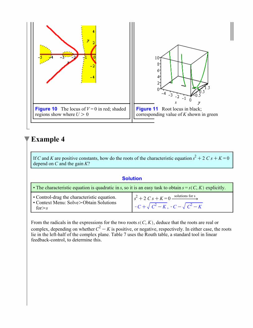
In Figure 10 the locus of roots ( is drawn in red, whereas the shaded regions indicate where . Hence, those portions of the red curves that lie within a shaded region belong to the root

locus. In Figure 11 the root locus is drawn in black, with the value of at each point on the locus shown in green.

Figure 10 The locus of in red; shaded regions show where

Figure 11 Root locus in black; corresponding value of shown in green

Example 4

If and are positive constants, how do the roots of the characteristic equation depend on and the gain ?

Solution

The characteristic equation is quadratic in , so it is an easy task to obtain explicitly.

Control-drag the characteristic equation.Context Menu: Solve_Obtain Solutions for_

solutions for s

From the radicals in the expressions for the two roots , deduce that the roots are real or complex, depending on whether is positive, or negative, respectively. In either case, the roots lie in the left-half of the complex plane. Table 7 uses the Routh table, a standard tool in linear feedback-control, to determine this.

Tools_Load Package: Dynamic Systems Loading DynamicSystems

Apply the RouthTable command to determine the number of zeros in the left-halfplane.

The number of such zeros equals the number of sign-changes (2) in the leftmost column.

=

Apply the RouthTable command to determine the number of zeros in the right-half plane.

The number of such zeros equals the number of sign-changes (0) in the leftmost column.

=

Table 7 Routh table used to determine the number of zeros in the left- and right-half planes

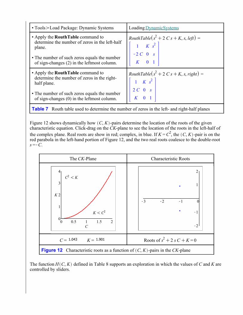
Figure 12 shows dynamically how -pairs determine the location of the roots of the given characteristic equation. Click-drag on the -plane to see the location of the roots in the left-half of the complex plane. Real roots are show in red; complex, in blue. If , the -pair is on the red parabola in the left-hand portion of Figure 12, and the two real roots coalesce to the double-root

.

The -Plane Characteristic Roots

1.043 1.901 Roots of

Figure 12 Characteristic roots as a function of -pairs in the -plane

The function defined in Table 8 supports an exploration in which the values of and are controlled by sliders.

Table 8 For each -pair, returns a graph of the corresponding roots of the characteristic equation

C: 0.75 1.5 2.25 3.00.00.000

K: 0.75 1.5 2.25 3.00.00.000

The calculations in Table 9 apply an additional Maple tool to the problem of determining the dependence of the characteristic roots on parameters. The CellDecomposition command in theRootFinding:-Parametric package creates a module containing a mix of features of the polynomial

system. In the context of feedback control, the characteristic equation is evaluated at , and separated into its real and imaginary parts, which, like the characteristic equation itself, must vanish. The additional inequality is added to the system to determine the number of roots in the right-half plane, a number that the control theorist would want to be zero. The parameter ranges that ensurethis outcome is then teased out of the module.

Initialize

In the characteristic equation, set , and separate into real and imaginary parts.

Using theCellDecomposition command, create the module .

Obtain the discriminant variety, a generalization of the discriminant for quadratic equations.

=

Interrogate for the number of solutions. There are two "cells" in the parameter space, numbered 1 and 2. Here, each such cell has zero solutions.

=

For systems with exactly two parameters, a graph showing the partitioning of the parameter space can be obtained with theCellPlot command.

Table 9 Sketch of the analysis of the characteristic equation made by the CellDecomposition command

Given a -pair, the characteristic equation determines a point on the root locus. Given apoint on the root locus, it is also possible to determine the -pair from which this point derives. This determination is simply a matter of solving the equations

for and . See Table 10 for an illustration.

0

Table 10 Determining and

In feedback control, standard practice for characteristic equations with more than one parameter, seems to be "fix all but one parameter and obtain the "root locus" for the one remaining parameter." Table 11 defines two functions that return a "root locus" when one of or is fixed, and the other parameter varies.

Table 11 Functions that draw a "root locus" when either or is fixed

Application of the Explore command to each of these functions results in a "root locus" in which the fixed parameter can be varied by a slider.

C: 2.5 5.01.25 3.750.01.000

K: 2.5 5.01.25 3.750.01.000

Either "root locus" implies that every point in the left-half plane is a solution of the characteristic equation for some pair of parameter values .

Example 5

If and are positive constants, how do the roots of the characteristic equation depend on and the gain ?

SolutionIn Example 4, the characteristic equation, quadratic in , could easily be solved for . In Example 5, although it is technically possible to solve the cubic characteristic equation, the expressions for the roots are so cumbersome that it is difficult to extract useful information from them. The benefit of a direct approach to understanding how the characteristic roots depend on the two parameters is not worth the cost.

Apply the Routh criterion

Tools_Load Package: Dynamic Systems Loading DynamicSystems

Apply the RouthTable command to determine the number of zeros in the left-half plane.

The number of such zeros equals the number of sign-changes (1) in the leftmost column.

=

Apply the RouthTable command to determine the number of zeros in the right-half plane.

The number of such zeros equals the number of sign-changes (2) in the leftmost column.

=

Table 12 Routh table used to determine the number of zeros in the left- and right-half planes

For all positive values of and , there is one root in the left-half plane and two in the right-half plane.

The function defined in Table 13 supports an exploration in which the values of and arecontrolled by sliders. It is illuminating to see that, indeed, there are always two characteristic roots in the right-half plane.

Table 13 For each -pair, returns a graph of the corresponding roots of the characteristic equation

C: 0.75 1.5 2.25 3.00.01.000

K: 0.75 1.5 2.25 3.00.01.000

Figure 13 provides the same information in a slightly different format. Here, a point in the -plane is selected and dragged in the pane on the left, and the corresponding characteristic roots

are graphed in the pane on the right.

The -Plane Characteristic Roots

1.487 1.058 Roots of

Figure 13 Characteristic roots as a function of -pairs in the -plane

The calculations in Table 14 apply the CellDecomposition command to the given characteristic equation. As in Example 4, set and separate the real and imaginary parts of the resulting form of the characteristic equation.

Initialize

In the characteristic equation, set , and separate into real and imaginary parts.

Using theCellDecomposition command, create the module .

Obtain the discriminant variety, a generalization of the discriminant for quadratic equations.

=

Interrogate for the number of solutions. There is but one "cell" in the parameter space, and it contains two solutions.

=

For systems with exactly two parameters, a graph showing the partitioning of the parameter space can be obtained with theCellPlot command.

Table 14 Sketch of the analysis of the characteristic equation made by the CellDecomposition command

By including the inequality in the CellDecomposition command, the number of zeros in the right-half plane is returned. There is just one cell in the parameter space, namely, the first quadrant ofthe -plane, and for that one cell, there will always be two solutions for which .

Example 6

Determine the root locus generated by the open-loop transfer function

.

(This transfer function appears on page 182 of [1]. The exponential arises from a time-delay in the feedback control system so modeled.)

Solution

Initializations

Tools_Load Package: Dynamic Systems Loading DynamicSystems

Set the imaginary unit to .

Define the open-loop transfer function .

The standard root-locus tools are restricted to rational functions.Instead, work directly with the characteristic polynomial.

Define the closed-loop transfer function .

Extract the characteristic polynomial, that is, the denominator of .

Solve the characteristic equation for the gain .

Set , obtaining .

Let and , respectively, be the real and imaginary parts of .

The root locus is the solution of and .

The red curves in Figure 14 are defined implicitly by .

The shaded regions in Figure 14 are the feasible regions for .

Hence, the red curves lying in the shaded regions of Figure 14 comprise this part of the root locus.

The trig functions introduced by the imaginary exponential endow the root locus with an infinite number of branches; Figure 14 shows just a few such curves. Figure 14 Root locus: red curves in shaded

regions

The function defined in Table 15 numerically solves the characteristic equation for specific values of , then superimposes the points so computed on the root locus in Figure 14. Note the use of the Analytic command in the RootFinding package. This command finds all solutions in a region of the complex plane, and has to be used instead of the fsolve command because the fsolve command finds all complex roots only for polynomial equations.

Table 15 A function that for given , superimposes on Figure 14

Applying the Explore command to the function adds to Figure 14, a slider that controls the value ofthe gain . As varies, the corresponding points on the root locus appear as black dots. This "animation" gives some sense of how points on the root locus are related to specific values of .

K: 15.05.0 20.010.00.05.000

Figure 14 shows that there are an infinite number of points where the root locus crosses the imaginary axis. The first three such points in the upper-half plane are found with the calculations in Table 16. Of course, symmetry implies that , are also on the imaginary axis.

= 0.1442450568

= 15.29164339

= 0.6632712390

=

= 1.274906850

= 978.3114712

Table 16 Some root locus points on the imaginary axis, and the corresponding gains

Standard practice in feedback control replaces the exponential in with a Padé approximation, thereby preserving the rational-function structure of the root-locus investigation.

Figure 15 compares, for real , the exponential with its Padé approximation. The exponential is shownin green; the approximation, in red.

Figure 16 makes the comparison for complex . Again, the exponential is shown in green; the approximation, in red.

Figure 15 Comparing and its Padé approximation for real

Figure 16 Real and imaginary parts of (green) and its Padé approximation (red). Real parts on the left; imaginary parts, on the right

In assessing the validity of the approximation, recall that every th-degree Taylor polynomial approximating the exponential has zeros, but the exponential itself has neither real nor complex zeros! So, while the approximation might be "good" for some domain, other essential properties might not be preserved.

Replacing in with the rational approximation leads to the approximate characteristic polynomial computed in Table 17.

Table 17 Exponential in approximated by a Padé approximation

Figure 17 is obtained by applying the RootLocusPlot command to , the approximation of the open-loop transfer function .

Figure 17 Root locus for , with

The root locus in Figure 17 entirely misses the periodicity seen in Figure 14. Moreover, it is qualitatively correct only in a small neighborhood of the origin.

References

[1]

Feedback Control of Dynamic Systems, Franklin, Powell, Emami-Naeini, Addison-Wesley Publishing Company, 1986.

[2] Control Systems Engineering, 4th ed., Norman Nise, John Wiley & Sons, 2004.

Legal Notice: © Maplesoft, a division of Waterloo Maple Inc. 2013. Maplesoft and Maple are trademarks of Waterloo Maple Inc. This application may contain errors and Maplesoft is not liable for any damages resulting from the use of this material. This application is intended for non-commercial, non-profit use only. Contact Maplesoft for permission if you wish to use this application in for-profit activities.