Introduction of DMSO into cell suspensions using a two-stream microfluidic device A THESIS SUBMITTED TO THE FACULTY OF THE GRADUATE SCHOOL OF THE UNIVERSITY OF MINNESOTA BY Rohini Bala Chandran IN PARTIAL FULFILLMENT OF THE REQUIREMENTS FOR THE DEGREE OF MASTER OF SCIENCE Prof. Allison Hubel December 2010
Transcript
Introduction of DMSO into cell suspensions using a two-stream microfluidic device
2.2 Configuration B: Buoyancy Induced Flow 16 2.2.1 Introduction: Equilibrium and departures from it 16 2.2.2 Flow model in Configuration B 17 2.2.4 Non-dimensional constants 20
collapsing and coinciding with model predictions, for fq = 0.23. (Standard Error = 4.1% for Co =
15% and 3.12% for Co = 10%) 39 Figure 4.4 (a) Cc* vs (1/Re) for an initial donor stream concentration of Co = 15% vol/vol and flow
rate fraction of fq = 0.23 for the flow configuration A, in which the donor stream is on top of
the cell stream. 42
Figure 4.5: Cc* as a function of (1/Re) for different donor stream concentrations (% vol/vol) using
flow configuration B; fq = 0.5 43
Figure 4.6: e* v/s (1/Re) for different flow rate fraction values of fq = 0.23, 0.5 and 0.77 for
Configuration B. 49
ix
List of Tables Table 1: Assumed values for DMSO diffusion and cell properties 14 Table 2 Significant dimensions of the two-stream microfluidic channel 25
Table 3 Atwood (At) and Rayleigh (Ra) numbers for various donor stream concentration values 47
Table 4 �umber density of the cells in the streams at the outlet of the channel for a fq = 0.5, Co =
15% for configurations A and B 52
1
Chapter 1
Introduction: Background, objectives and overview
1.1 Background: Cryopreservation of cells and its significance
Biological cells are used for fundamental studies of physiological and pathological
functions and for diagnostic, therapeutic, and epidemiologic purposes. These cells need
to be preserved and stored so that they can be used, whenever needed, for a variety of
applications in medicine and biotechnology. Typically, cells are cryopreserved despite
popular debates owing to the toxicity of certain cryoprotective agents[1-3]. Due to
freezing during cryopreservation, biochemical reactions that occur in the cells are
drastically reduced. As the cell membrane in cells are effectively semi-permeable, i.e.
impermeable to many solutes but permeable to water, with freezing, the extracellular
solution effectively starts to become more and more concentrated and water therefore
leaves the cell until the gradient in chemical potential is neutralized to restore osmotic
equilibrium. This movement of water molecules in addition to the ice crystal formation
within the cells during freezing results in cell injuries, the minimization of which is an
area of active research. Effective methods of preserving cells typically require the use of
cryoprotective agents (CPAs), molecules that act to protect cells from the stresses of
freezing and thawing [4] .The most commonly used is dimethyl sulphoxide (DMSO), a
penetrating cryoprotective agent (CPA) that reduces ice formation in the cells by
dehydrating the cell before freezing [5]. Cells respond to this change in environment with
rapid changes in cell volume as water leaves the cell followed by penetration of the CPA.
These volumetric excursions, if significant enough, can result in cell lysis. Conventional
protocols for addition of CPAs into cell suspensions typically involve the use of step-
wise introduction or syringe pumps designed to gradually increase the extracellular
concentration and thereby minimize volumetric excursions and cell losses. Cell losses
due to osmotic stresses can be observed both during introduction and removal of
cryopreservation solution. A study of the effects of CPA osmolality on sperm motility
has been studied and the importance of optimal procedures for introduction and removal
2
of CPA into cells has been stressed by Guthrie in [6]. The target concentration of DMSO
that needs to be introduced varies depending on the cell types, although most standard
protocols suggest introducing 10% (v/v) DMSO[3]. Recent studies have shown the
success of using different combinations and concentrations of CPAs for cryopreservation
of cells such as Clapisson, who uses a mixture of 3% HES (hydroxyl ethyl starch) and
5% DMSO for cryopreservation of peripheral blood stem cells (PBSC) [7] For the sake of
this project, we set our target to introduce 10% DMSO in a cell suspension using a two-
stream microfluidic channel that was developed by Fleming, Mata, et. al [8, 9]
1.2 Two stream microfluidic channel: Review and results from prior
work
The applications of microfluidic devices are widespread, especially in the medical device,
industry, and are reviewed in detail by Beebe et. al [10] . Some of the established and
well-known advantages of using micro-scale devices are the following:
• Flexibility to processing small volumes of fluids
• Low volume of manufacturing materials resulting in reduced costs.
• Portability and easy integration of parts for automated control.
Also, the physical phenomena that dominate at the microscale are very different from
what would otherwise be observed for larger dimensions. We observe laminar flow
patterns due to small sizes of the channel and an order of magnitude increase of surface
area to volume ratio when going from macro to micro scale and hence heightened surface
effects of viscosity and adhesion. It is hence challenging to explore new avenues of the
governing physics to effectively control fluid and cell motion in a micro-channel..
Recently, we demonstrated the ability to use microfluidic channels for the effective
removal of DMSO from a cell stream [8, 9, 11]. These studies demonstrated that Peclet
number and flow rate fraction are critical modeling/design factors in the removal of
DMSO from a cell stream. These studies demonstrated our ability to characterize
mathematically the transport of CPAs out of the cell stream and this behavior was
validated experimentally [8, 9]. We also demonstrated our ability to control, characterize
3
and visualize cell motion in the channel [9]. Fleming’s dissertation addresses, in
extensive detail, the following aspects and applications of the designed microfluidic
channel:
1. Predictive numerical and computational models to determine the transfer of DMSO
between the two streams in the channel, particularly focusing on extracting DMSO
from the cell stream into a wash stream. Specifically, her models incorporate both
intracellular and extracellular diffusion that takes place in the cell stream
2. Experimental validation for the diffusion-based removal model for various flow
conditions in the channel. [8, 9]
3. Theoretical models and experimental data for optimization of the design of the
device in order to process clinical-scale volumes. [12]
Although, the diffusion model in [8, 9] has been generally extended to understand the use
of the device for introducing DMSO into the cell stream, the study is only preliminary
and full - fledged experimental validation/characterization for various flow and operating
conditions has not been done. Based on the model results for introduction of DMSO,
using the microfluidic device, two vital issues can be identified:
1. To achieve the target 10% DMSO concentration at the outlet for the cell stream, in the
regular set up of having the heavier and richer donor stream flowing in the bottom of the
channel, we require high initial donor stream concentrations ( > 15%) if we are looking to
process clinical scale volumes ( ~ 1 – 2.5 ml/min) in the designed channel. Such large
donor stream concentrations are detrimental to the recovery of the cells [5] as well as
reliable device behavior.
2. Also, the effect of gravity has been neglected in Fleming’s [13] numerical and
experimental removal models. For the purpose of introduction of DMSO, since the CPA
molecules and the cells are in different streams, resulting in significant density contrasts
(7x10⁻⁴
< At <7x10⁻³
), it becomes imperative to incorporate the effects of gravity in
understanding flow behavior and cell motion in the device.
1.3 Objectives and Significance
In this dissertation, it is intended to investigate the transfer of DMSO, from a donor
stream that is rich in CPA concentration to a cell suspension, using the two-stream
microfluidic device for two different flow configurations of the fluids within the device.
4
One configuration has the heavier donor stream in the bottom and the cell stream on the
top and vice-versa for the alternate configuration. Due to the differences in densities of
the fluids in the channel, the role of gravity in mass transfer and cell motion cannot be
undermined. Consequently, another significant objective of my work is to understand the
influence of gravity in mixing two miscible fluids of varying densities in a micro channel,
with an externally imposed bulk flow in the transverse direction owing to the driving
pressure gradient. It is intended to test if gravity can be used as an added
potential/driving field to produce effective mass transfer of CPA molecules from the
donor to the cell stream.
A variety of methods have been used to introduce chemicals into a stream or mix two or
more streams of different compositions using microfluidic devices. These methods
include passive methods such as simple diffusion [14] or micromixing using obstructions
[15] and active methods such as mixers driven by electrosomotic flows [16], that takes
advantage of electric field fluctuations to produce mixing ; acoustic attenuation induced
body forces used by J.C. Rife et. al in [17] ; thermal effects [18]; magnetic [19]and
centrifugal forces to produce high speed micromixing [20]. Excellent reviews of the
main issues associated with mixing at the microscale and diverse methods to cause
mixing are provided by Julio M. Ottino and Stephen Wiggins [21] and Elmabruk A.
Mansur, YE Mingxing et. all [22]. All applications studied to date have either used
dilute systems (e.g. the concentration of solute to be mixed is low) and the different
stream exhibited largely the same density. In contrast, Yoshiko Yamaguchi et. al [23]
have studied the effects of gravity in a micro channel using numerical simulations and
confocal microscopy of blood serum with a phosphate buffer solution. They use the
interface tilt angle as a rough estimate of flow behavior in the system and establish its
dependence on a dimensionless parameter, which is a function of density difference,
average velocity, viscosity and geometry of the channel, assuming negligible diffusion
effects. The novelty of this work is reflected in the fact that the effects of buoyancy and
the physics of interactions of two miscible fluids of varying densities in a micro-channel,
with a superimposed velocity perpendicular to the force of gravity, has not been
understood and modeled so far.
5
Rayleigh-Taylor instabilities [24] can develop when a dense fluid overlies a lighter one.
The stability of such an interface between two superposed fluids of different densities
was studied by Rayleigh and Taylor [25] and further numerical analysis was done by
Chandrasekhar[26]. Figure 1.1 shows the characteristic shape of R-T mixing of two
miscible fluids (cold and warm water) in a water tunnel experiment, captured by planar
laser induced fluorescence imaging, for a small Atwood number of 7.4 *10-4
. According
to [27], the spikes of the heavy fluid and light bubble penetrate symmetrically at the
density interface for small Atwood number scenarios. This is relevant to us as our
experiments in the channel fall in the category of At << 0.1. Gravity currents and flows
driven by buoyant convection are important especially in relation to large physical
systems such as, mixing of salt and fresh water in oceans, heat transfer from the ground
to the atmosphere, etc. Quantitative numerical models of fluid motion have been
developed typically for a vertical geometry where in flow direction is parallel to that of
forces due to gravity, such as plumes, capillary tubes [28]. Also, these processes have
been modeled for unconfined geometries [29], where in physical mechanisms of
viscosity and/or diffusivity, depending upon the configuration, have been neglected. In all
of these problems, pertinent dimensionless constants such as the Rayleigh number [30],
Graschof number [31], etc. serve as yardsticks to compare the relative significance of
free convection due to buoyancy over any other forces that my act in the system. For
instance, the importance of Atwood number (At) in determining different flow regimes
and an analysis of buoyancy driven front dynamics in tilted tubes has been presented by
Seon and his group [32]. They discuss the effectiveness of mixing in such flows
depending on the viscosity of the fluids, Atwood number and the geometric configuration
of the tube.
6
1
Figure 1.1 Shape of R-T mixing for small Atwood numbers
In this work, we attempt to characterize dimensionless quantities such as Atwood
number (At) and Rayleigh number (Ra), to classify the nature of flow and the
effectiveness of mixing, insofar as possible by using a solution of PBS (phosphate-
buffered saline) in conjunction with the donor stream, for the alternate flow
configuration. (Configuration B)
The broad objectives of this project can be summarized as below:
• Use the already designed two-stream microfluidic channel to introduce a target DMSO
concentration of 10% (v/v) in a cell suspension for two different flow configurations in
the channel
• Understand the effects of gravity for the flow configuration where the heavy donor
stream flows on top of the lighter fluid in the channel.
• Investigate cell recovery, number distribution and cell motion for both configurations in
the channel.
• Characterize and visualize cell motion for both these configurations within the channel to
understand better the flow physics involved.
1.4 Overview of dissertation
As already stated, the overall goal of this project is to use the two-stream microfluidic
channel to introduce a 10% (v/v) of dimethyl sulfoxide into a cell suspension while
1 Adopted from the review on Small Atwood number Rayleigh-Taylor Experiments 27. Dalziel,
M.J.A.a.S.B., Small Atwood number Rayleigh-Taylor experiments. Phil. Trans. R. Soc. A, 2010. 368: p. 1663-
1679.
7
understanding different flow configurations and buoyancy effects due to gravity in the
channel. The flow of content in this document is briefed as below. The subsequent
chapter introduces the reader to the numerical and computational modeling for
determining the concentration of DMSO at the exit of the device and brings to light the
changes that are made to incorporate the time delay in diffusion due to the presence of a
membrane in the cells. Furthermore, the important dimensionless parameters such as
Peclet number (Pe), flow rate fraction (fq), cell volume fraction (CVF), Atwood number
(At) and effectiveness of mass transfer (e*) have been discussed in depth in this chapter.
Chapter 3 elaborates on the experimental set-up and the methods followed to conduct
experiments for the different flow configurations, procedure to perform
spectrophotometry for concentration analysis and discuss information about the
visualization studies with the cells. The next chapter presents the results obtained,
focusing on the concentration profiles at the outlet of the cell stream for different flow
rates and flow rate fractions of the fluids in the channel. Again, this has been done for
both the flow configurations and a detailed discussion supports why we observe different
results in these configurations. In particular, a shift of the nature of the mass
transfer/mixing mechanism has been identified based on the density contrasts for the
alternate configuration in the channel. Selected results from the experimental trials with
cells and a comparison study for the distribution of cells in the two streams has been
included in this chapter. Finally, the last chapter summarizes the work that has been done
in this project, the inferences and conclusions that can be made from the results obtained
thus far and recommends directions for future work towards the goal of using
microfluidic devices to effectively introduce DMSO into a cell suspension. A discussion
about the limitations and scope of this dissertation work has been incorporated in this
final chapter.
Well, now let’s begin!
8
Chapter 2
Numerical modeling and dimensional analysis
As already discussed, the two-stream microfluidic device that was used by Fleming et. all
[13] for the removal of DMSO, is used to introduce DMSO into a given cell suspension
in a gradual fashion along the length of the channel in order to minimize osmotic shock
on the cells. The general schematic (Fig. 2.1a and Fig 2.1 b) of the device consists of two
streams flowing in parallel allowing for the transport of DMSO molecules to the cell
suspension. The terminology for the streams flowing in the device is as follows:
(a) Donor stream , consisting of DMSO in phosphate buffered solution (PBS) and as a
result heavier than just PBS solution
(b) Cell stream, which is phosphate buffered solution (PBS) which may or may not contain
cells. .
Two flow configurations of fluids in the device have been studied in this dissertation.
Configuration A, where in the donor stream flows in the bottom and the cell stream is on
the top (Figure 2.1a) and Configuration B (Figure 2.1b), which has it exactly reversed
with the donor stream on the top. The relative depths of each of these streams can be
chosen arbitrarily, the effects of which is discussed at a later section.
Figure 2.1: General flow schematic in a two-stream microfluidic device with two streams
entering at the left with different volume flow rates (denoted by qc and qd) wherein (a)
Configuration A with donor stream in the bottom (b) Configuration B with donor stream on the
top
9
2.1 Configuration A: Numerical Model
Mathematical modeling for the introduction of DMSO in this configuration has already
been discussed by Fleming [13]. Let us first consider a case for which the cell stream
doesn’t contain any cells and understand the essence of her modeling methods and
parameters.
2.1.1 Acellular modeling
For flow configuration A, the transport of DMSO from the donor stream to the cell
stream can be assumed to take place via diffusion and is modeled as:
( ) 2DC D C
Dt= ∇ … (2.1)
where,
C – concentration of DMSO (vol /vol)
D – diffusion coefficient or diffusivity of DMSO in PBS
The following assumptions have been made about the flows in the channel:
1. Steady two-dimensional flow of the fluids.
2. The variation in viscosity of the fluids has been neglected in the modeling.
3. Due to the high value of Sc (Schmidt number, ScD
ν= ,
3~ (10 )Sc O , where ν -
kinematic viscosity; D – diffusivity of DMSO), a fully developed velocity profile can be
assumed.
4. No effect of gravity in this configuration of flow in the channel.
Appendix A.1 presents the derivation of the velocity profile based on the above
assumptions by solving the Navier-Stokes equation for a constant pressure gradient in the
X-direction. The high value of Sc implies that the Navier-Stokes equations can be
decoupled from equation (1) and can be reduced to
2 2
2 2( )
C C Cu y D
x x y
∂ ∂ ∂= + ∂ ∂ ∂
... (2.2)
10
where-in u(y) is obtained from Navier-Stokes equations and is given by a parabolic
profile (refer Appendix A.1) as follows
( )2( )2
g
du y P y yd
µ= − − … (2.3)
gP -Pressure gradient in X-direction; d – depth of the channel, µ - dynamic viscosity of
the fluids. Note that this equation is used when the cells aren’t present in the streams.
When cells are introduced in the channel, we need to account for the diffusion of DMSO
molecules from the extracellular solution to the intracellular solution, due to the presence
of physical barrier in the form of a cell membrane. A detailed time constant analysis, for
diffusion across the cell membrane based on cell properties (membrane permeability P,
membrane thickness Mth) and diffusion of DMSO in the extracellular space, has been
presented by Fleming. [13]
2.1.2 Cellular modeling
DMSO is a small enough molecule that it can diffuse inside the cell. The rate equation
for the transport of DMSO molecules across the thickness of the cell membrane is given
by
( )ie i
dCB C C
dt= − ... (2.4)
Owing to steady flow assumptions, this equation now reduces to
( ) ( )ie i
Cu y B C C
x
∂= −
∂ … (2.5)
The resulting modifications to equation 2.2 due to the presence of cells is presented
below
2 2
2 2( )
( ) ( )
ii e
t
V BC D C CC C
x u y x y V u y
∂ ∂ ∂= + + − ∂ ∂ ∂
… (2.6)
where the concentration Ce is the number of moles of extracellular DMSO per local
extracellular volume, Ve, Ci is the number of moles of intracellular DMSO per
intracellular volume, Vi, Vt is the total volume, and B is the modeling membrane
permeability to DMSO (calculated by dividing the cell membrane permeability, P, by the
thickness of the cell membrane, Mth: B = P/Mth). 2.5 and 2.6 need to be simultaneously
solved to obtain the concentration distribution within (Ci) and outside (C) of the cells.
11
2.1.3 Scaling Analysis
Equation 2.6 is scaled in order to obtain significant dimensionless parameters influencing
the flow and concentration profile of the fluids in the channel. Using a mean velocity
value - avgU , channel depth d, length L and an initial donor stream concentration of Co,
the scaling equations can be written as:
* * * * * *; ; ; ; ;i e
i e
avg o o o
C Cu C x yu C x y C C
U C L d C C= = = = = =
Applying this transformation to eqn. 2.2, we obtain
2 2
2 2 2 2
* 1 * 1 **
* * *avg
C DL C Cu
x U L x d y
∂ ∂ ∂= + ∂ ∂ ∂
Since L >> d, the cross stream variations can be assumed to be much stronger than along
the stream 2 2
2 2
* *
* *
C C
y x
∂ ∂>> ∂ ∂
and the first term in R.H.S can be neglected. Therefore, the
equation above reduces to
2
2 2
* **
* *avg
C DL Cu
x U d y
∂ ∂= ∂ ∂
… (2.7)
Using this result in 2.6 and scaling all length dimensions with respect to the channel
depth, d, we get
2
2
* *( * *)
* *
ii e
avg t avg
V BdC Dd CC C
x U y VU
∂ ∂= + − ∂ ∂
… (2.8)
The following dimensionless constants can be derived from the scaling analysis presented
above.
Peclet number
This dimensionless parameter is a measure of relative importance of advection and
diffusion in the channel. Two different Peclet numbers can be defined for this problem,
PeL (based on the length of the channel) and Ped, based on the depth of the channel. Ped is
of more relevance and is evident from the scaling analysis above and will be referred to
as Pe from here on.
12
avgU d
PeD
= … (2.9)
Peclet number is relevant in our discussion for this configuration due to convection and
diffusion being the only dominating forces acting in the system.
The coefficient of the diffusion term on the right hand side of the (2.7) is the ratio of time
constants for convection ( convτ ) defined as conv
avg
L
Uτ = and diffusion (
diffτ ), given as,
2
diff
d
Dτ = . Higher this value, higher is the time constant for convection and hence more
prominent diffusion effects in the channel. This coefficient can be thought of as a
dimensionless length and given as 1 L
Pe d
(2.10).
*avg
BdB
U= (2.11a) and
t
i
V
V(2.11b) are apparent dimensionless parameters from the scaled
equation in 2.8. Notice that the mean velocity avgU may be expressed in terms of qt and
the channel cross sectional area:
tavg
qU
dw=
Flow rate fraction
An independent parameter, d
δ, resulting from the initial conditions of the relative depths
occupied by the fluids in the channel and is related to the inlet flow rate fraction fq, which
is defined as
cq
t
qf
q= … (2.12)
where qt = qc + qw is the total volumetric flow rate through the channel. Here, qc and qw
are the cell stream and wash stream flow rates, respectively. The flow rate fraction fq is
related to δ /d, where δ is the depth of the channel occupied by the cell stream, as
13
2 3
3 2qfd d
δ δ = −
… (2.13)
The above derivation is obtained based on a parabolic velocity profile of the fluid flow in
the channel. The derivation of the same is presented in Appendix A2.
The flow rate fraction directly affects the maximum attainable equilibrium concentration (
eqC ) at the outlet of the channel, which is given by
( )1eq q oC f C= − … (2.14)
Therefore the limit for the maximum attainable concentration of DMSO in the cell stream
is the normalized equilibrium concentration and this limit is referred as the introduction
limit.
( )* 1eq
eq q
o
CC f
C= = − … (2.15)
Reynolds number
The Reynolds number is another dimensionless parameter, which represents the ratio of
inertial and viscous forces for the fluid. For this system, the Reynolds number Re is
defined as
µρUd
=Re … (2.16)
where ρ is the density of the liquid and µ is the dynamic viscosity of the fluid. In our
studies, the range of Reynolds number varies from 0.7 – 7, and as a result flow in the
channel could be considered creeping flow with viscous forces dominating the inertial
forces. For the investigation in Configuration B, the inverse of the Reynolds number
(1/Re) is representative of a non-dimensional residence time for the fluid in the channel.
Table 1 below lists the values of the various constants used in developing the numerical
model for Configuration A.
14
Table 1: Assumed values for DMSO diffusion and cell properties
Constants and Properties for �umerical Model
Symbol Property Value
D
Diffusion Coefficient
800 µ m2/sec
µ Dynamic viscosity 1.112E-3 kg/m-s
P Membrane
Permeability 9.4 ( µ m/min)
B Cell Modeling
Permeability 3-15 (1/s)
V2 Cell Volume 2144 ( µ m3)
dc Cell Diameter 16 ( µ m)
A Cell Surface Area 805 ( µ m2)
t Membrane thickness .01-.05 ( µ m)
2.1.4 Computational method
Finite difference method is used to solve the numerical equations (2.3,2.7) in MATLAB
(Mathworks, MA). Fleming [13] has used a forward marching in X-direction and a
central difference in Y-direction, explicit, finite difference method in her approach to
solve the equation. (Refer Appendix A3). The stability of an explicit finite difference
formulation is questionable, especially for varying values of velocity (u(y)) in 2.7 (donor
stream) and 2.8 (for the cell stream) is of a big concern at low velocity values [33].
Therefore, the grid spacing needs to be adjusted accordingly to obtain the results,
especially for slower flow rates of the streams in the channel. To address this problem, a
backward time central space, Laasonen finite difference method was developed for the
acellular model which is consistently stable for any value of the average velocity in the
channel and the algorithm and implementation of the code has been attached in Appendix
A3.
15
As we are solving a parabolic equation, we need to list the initial and the boundary
conditions that need to be specified to obtain a solution to the problem, i.e. determining
the outlet concentration of the fluids for a given length of the channel.
Initial Conditions
• Concentration Field
• Velocity Field
A uniform parabolic velocity profile for the fluids has been assumed and is given by
( )22
2g
d y yu y P
d dµ
= − − … (2.17)
where gP is the constant pressure gradient in the X-direction offered by the syringe pump
driving the fluids in the channel. The derivation of the relationship between gP and
avgU , the average mean velocity of flow in the channel, is given in Appendix A1 and
can be written as
12; width of channel
avg
g
UP w
dw
µ= − … (2.18)
Boundary Conditions
• Concentration Field
There is no flux at the walls of the microfluidic channel and this condition is
given as
0 for 0,C
y y dy
∂= = =
∂
• Velocity Field
A no-slip boundary condition is imposed in the walls of the channel as the viscosity of
the fluid is important. Hence,
( ) 0 for 0,u y y y d= = =
The mesh size needs to be chosen appropriately in order to obtain a good solution to the
equation. The values of x∆ and y∆ are usually estimated based on a grid independence
( )
o
0, for 0
0 for
C - initial donor stream concentration
oC y C y d
d y d
δ
δ
= < ≤ −
= − < ≤
16
test and if the explicit method is used to solve 2.7, the stability criterion must also be
satisfied [33]. This equation is then solved for the concentration field at all the nodes
and the final outlet concentration of the two streams at the outlet of the channel can be
obtained for various flow rate values (Pe) and flow rate fractions (fq). Concentration
plots for the above developed theoretical model have been presented in Chapter 4 along
with the other experimental results.
2.2 Configuration B: Buoyancy Induced Flow
In configuration B, the dense and the DMSO-rich donor stream lies on top of the cell
stream resulting in density gradients along the depth of the channel in the Y-direction.
Hence we need to account for effects of gravity in the flow patterns as well as the
mechanism of DMSO exchange between the fluids since it is not only diffusion which
acts to redistribute the concentration of DMSO molecules, but the buoyant forces can also
potentially cause movement of these molecules owing to the density gradient in the
channel. In such cases, when gravity acts in concurrence with density gradients,
convection effects will be observed in a system. The study of influence of
buoyancy/density stratification in horizontal/parallel flows, especially produced by
temperature differences, dates back to the classic problem of thermal natural convection
to determine the nature of flow between horizontal plates uniformly heated from
below[30]. Buoyancy effects in fluids and the stability analysis of inviscid plane flows
have been analyzed by Drazin and Howard (1966).
2.2.1 Introduction: Equilibrium and departures from it
In general, buoyancy forces results from variations in density that can be caused due to
inhomogeneities in temperature, concentration of chemical species, change of phase and
many other effects. A body of homogenous, inviscid, incompressible fluid at rest in a
state of neutral equilibrium since at every point, the weight of the fluid is balanced by the
pressure exerted on it by the neighboring fluid. When ρ varies, either in the same fluid or
due to density contrasts between different fluids, this equilibrium will be affected by the
density distribution or stratification. The equilibrium will be stable when the heavy fluid
lies below (Figure 2.2a), since the tilting of the density interface will produce a restoring
force resulting in oscillatory motion. A pressure mismatch exists at the interface when the
17
heavier fluid is on top of the other, which acts to reorient the streams to restore the low
potential energy configuration (Figure 2.2 b)
2
Figure 2.2: Displacements from equilibrium: (a) Stable (b) Unstable density distribution
2.2.2 Flow model in Configuration B
Configuration B in the channel, where in the heavier donor stream is on top of the lighter
cell stream, presents a case of unstable density stratification of miscible fluids with an
imposed pressure-driven mean flow in the X-direction.
The following assumptions have been made to ease the complexity of the problem:
• The two fluids are miscible and there is no distinct interface between the two streams
resulting from interfacial free energy
• We are interested in the flow properties and concentration field at the outlet of the device,
which is more than hundreds of the diameter of the channel, i.e at late times and hence
assume steady flow.
• Since the Reynolds number is of O(10), we have assumed 2-D flow inside the channel.
Driving potential
In the microfluidic device, when being operated in the alternate configuration B, the
concentration gradient (translates directly to a density gradient as density is a function of
concentration as given in 3.4) between the solutions result in convection or flow,
popularly referred to as free convection. In fact, the net body force, B ( B gρ= ∆ ; ρ∆ -
density difference of the fluids) is a driving force/potential acting on the miscible fluids
flowing in the channel, like any other external (electric/magnetic/chemical) potential that
may/may not enhance mixing of the fluids in the channel.
2 Adopted from Turner’s notes on Pg. 30. J.S.Turner, Buoyancy Effects in Fluids. 1973.
18
Force Analysis
In our channel in Configuration B, the following are the dominating forces that act to
affect the fluid motion within the channel:
• Driving force (B ~ gdρ∆ ) of buoyancy, B, as derived above, which would cause the
heavy donor molecules to drop down into the lighter stream,
• Viscous force (Fv
2
~V
d
µ) , , where V is the characteristic viscous(?) velocity in the Y-
direction. Viscous forces are expected to stabilize and retard the downward motion of
the heavy DMSO molecules,
• Diffusion (Fd 2~
DV
d
ρ) which will act to diminish the concentration gradient across the
depth of the channel
• Bulk convection (Fu2~ avgUρ ) forces that affect the overall residence time and hence
influence the domination of one of the above forces over the other.
Figure 2.3 Directions of forces acting in flow configuration B
Transport Equations and Boussinesq approximation
The general transport equation for the fluids in the channel is given by Navier-Stokes
equation with the specific difference of including the changing body force per unit
volume as compared to the earlier model developed in the 2.1. This body force makes the
flow field two dimensional and more complicated to adopt a direct solution methodology
as in the former scenario.
The inlet density profile of the fluids is given as
19
( ) 1
2
0 y
y
y d
ρ ρ δ
ρ δ
= ≤ ≤
= < ≤
where, 2 1ρ ρ>
A linear relation exists between density and the concentration of DMSO in the stream
(Section 3.1) implying that
, where k is an arbitrary constantkc
ρ∂=
∂
Continuity
. 0D
VDt
ρρ+ ∇ =
��
���� ��
Assuming steady-state, this equation reduces to
( ). 0Vρ∇ =�� ��
… (2.19)
Momentum Transport
2DVp g V
Dtρ ρ µ= −∇ + + ∇
��
… (2.20)
The local quantities in the above equations are explained in Nomenclature section.
1 'ρ ρ ρ= +
where 'ρ - local density variations due to concentration differences.
Therefore the maximum possible density variation is given as:
2 1ρ ρ ρ∆ = − … (2.21)
The approximation introduced by Boussinesq (1903) consists of essentially neglecting
variations of density in so far as they affect inertia, but retaining them in the buoyancy
terms where they occur in combination with gravity (g).
2
1 1 1 1
' '1
DV pg u
Dt
ρ ρ µρ ρ ρ ρ
∇+ = − + + ∇
��
… (2.22)
Since 1
'ρρ
<< 1, the only term that changes from 2.21 is the term with the force due to
gravity.
20
With direct pertinence to the model for the microfluidic device, the following
assumptions can be made about the flow:
• Flow is two dimensional; ( ) 0z
∂=
∂
• Steady flow of the fluids in the channel and therefore ( ) 0t
∂=
∂
Therefore, expanding the above equations we have:
2 2
2 2
1 1
2 2
2 2
1 1
0
1
'
u v
x y
u u p u uu v
x y x x y
v v v vu v g
x y x y
µρ ρ
ρ µρ ρ
∂ ∂+ =
∂ ∂
∂ ∂ ∂ ∂ ∂+ = − + + ∂ ∂ ∂ ∂ ∂
∂ ∂ ∂ ∂+ = + + ∂ ∂ ∂ ∂
… (2.23)
This two-dimensional flow field needs to be solved by using a pressure-
correction/vorticity-stream function method and would involve significant computational
power to obtain fine mesh sizes to capture the physics of low Reynolds number flows.
This can be done using a software based solver or an originally developed optimized code
to solve the set of equations. In this project, these equations are not actually solved, but
then, we obtain dimensionless or scaling constants that are helpful to compare the relative
importance of the various forces driving the fluid motion and mass transfer of CPA in the
channel. This doesn’t mean that the previously developed constants in the section 2.1.3
don’t hold any significance but rather implies that we need to define other non-
dimensional quantities to characterize the extent of influence of gravity in the
microfluidic channel. In the subsequent section, dimensionless constants typically used in
natural convection (free convection due to buoyancy) have been discussed and the
relevance of these constants in our problem has been eventually brought to light in
Chapter 4.
2.2.4 Non-dimensional constants
It is to the benefit of modeling that a direct analogy can be set up between concentration
and temperature fields for a given system. Although the fluid motion in Configuration B
21
cannot be deduced to a pure natural convection based mass transfer, it is a valuable
exercise to understand the governing dimensional and scaling laws in natural convection
induced by thermal gradients. Some of the important dimensionless constants pertinent
to natural convection problems are discussed below.
Rayleigh number
This investigation examines flow/transport driven by differences in density. The ratio of density
driven flow divided by viscous forces is the Grashof number (Gr), given by
3
2
gdGr
ρρν
∆= [31].
But, this assumes that there is no bulk motion of the fluid in the X-direction, i.e. avgU =0.
Transport in the channel may also be influenced by diffusion and the Rayleigh number may also
be relevant. The Rayleigh number is defined as.
3
*
Ra Gr Sc
gd
D
ρρν
=
∆=
(2.24)
where Sc is the Schmidt number and ρ can be taken as the density of the heavier fluid in
the channel. Therefore the Rayleigh number reflects the relative importance of buoyancy
with respect to viscosity and diffusivity. Critical values of Ra for different flow situations
and geometric configurations has been provided in the discussion on free convection by
Cussler [34] which would help determine the onset of free convection in the given
system. Such constants cannot be directly incorporated as threshold values in our system
as
Atwood number
Atwood number is an estimate of the density differences between the two streams and is a key
factor in governing the growth rate of Rayleigh-Taylor instabilities [24]. Andrews and Dalziel
discuss its significance in directly affecting the effectiveness of mixing in a given system{Dalziel,
2010 #59. The Atwood number is given by
2 1
2 1
At ρ ρρ ρ
−=
+
… (2.25)
22
Variance of cell stream concentration (e) and Effectiveness of mixing/mass transfer
(e*)
In view of being able to quantify the extent of mixing or the lack thereof for various flow
conditions in Configuration B, we introduce a variance parameter e. There is a certain
limit for the maximum attainable equilibrium concentration (eqC ) for a given donor
stream concentration and a flow rate fraction value and we have derived this 2.15.
Ideally, we would like to reach the introduction limit for the cell stream at the outlet of
the channel. The deviation of the cell stream concentration from the equilibrium
concentration is given by the variance parameter (e) has been defined and is given by
( )2
c eqe C C= − … (2.26)
A normalized dimensionless effectiveness coefficient of mass transfer/mixing (e*), is
developed based on e, in the following fashion
*
max
1e
ee
= −
… (2.27)
where,
( )2 2
min max0; 1 oe e fq C= = −
… (2.28)
Here, mine is the minimum value of deviation from equilibrium and maxe is the maximum
deviation possible in the concentration of the cell stream. Therefore, higher the value of
e*, lesser is the variance/deviation from the equilibrium concentration value and more
effective is the equilibration of the two streams in the device. Taking into account, the
average standard experimental errors (~5-8%), Cc* within 10% (i.e, for Cc* = 0.9 Ceq*)
of the value of Ceq* can still be considered as an equilibrium condition and this is backed
by Fleming’s arguments well {Katie, 2008 #8}. Hence we define a threshold value for
effectiveness of mixing coefficient given by thε , i.e the value above which mixing can
be considered homogenous inside the channel. The derivation is as below for obtaining
thε
Substituting * *0.9c eqC C= in Equation 2.26 we get,
23
( )2
0.1 eqe C=
… (2.29)
From 2.27, we have,
( )2
max
1 q o eq
eq
f C C
e C
− =
⇒ =
… (2.30)
Combining 2.27, 2.29 and 2.30 we can compute the threshold value as
micromixer. Chem. Eng. Technol., 2005. 28(5): p. 613-616.
21. Julio M. Ottino, S.W., Introduction: mixing in microfluidics. Philos Transact A
Math Phys Eng Sci., 2004. 362(1818): p. 923-35.
22. Mansur, E.A., et al., A State-of-the-Art Review of Mixing in Microfluidic Mixers.
Chinese Journal of Chemical Engineering, 2008. 16(4): p. 503-516.
23. Nakamura, H. and et al., Influence of Gravity on Two-Layer Laminar Flow in a
Microchannel. Chemical Engineering & Technology, 2007. 30(3): p. 379.
24. Sharp, D.H., An overview of Rayleigh-Taylor instability. Physica D: Nonlinear
Phenomena, 1984. 12(1-3): p. 3-10, IN1-IN10, 11-18.
25. Taylor, G.I., Proceedings of the Royal Society of London, 1954(Series B): p.
67,857.
26. Chandrasekhar, S., Hydrodynamic and Hydromagnetic Stability. 1961, Oxford:
Clarendon Press.
27. Dalziel, M.J.A.a.S.B., Small Atwood number Rayleigh-Taylor experiments. Phil.
Trans. R. Soc. A, 2010. 368: p. 1663-1679.
28. Debacq, M., et al., Buoyant mixing of miscible fluids of varying viscosities in
vertical tubes. Physics of Fluids, 2003. 15(12): p. 3846-3855.
29. V. K. Birman, B.A.B., E. Meiburg and P. F. Linden, Lock-exchange flows in
sloping channels. J. Fluid Mech. (2007), 2007. 577: p. 53-77.
30. J.S.Turner, Buoyancy Effects in Fluids. 1973.
31. R.Byron Bird, W.E.S., Edwin N Lightfoot, Transport Phenomena. 1963.
32. T. Séon, J.-P.H., D. Salin, B. Perrin and E.J. Hinch, Buoyancy driven miscible
front dynamics in tilted tubes. Physics of Fluids, 2005. 17(3): p. 031702.
33. Klaus A Hoffman, S.T.C., Computational Fluid Dynamics. Vol. I.
34. E.L.Cussler, Diffusion Mass Transfer in Fluid Systems.
35. Abrahamsen JF, B.A., Bruserud Cryopreserving human peripheral blood
progenitor cells with 5-percent rather than 10-percent DMSO results in less
apoptosis and necrosis in CD34+ cells. Transfusion. 44(5): p. 785.
60
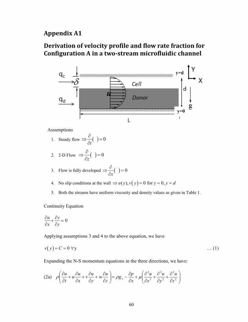
Appendix A1
Derivation of velocity profile and flow rate fraction for
Configuration A in a two-stream microfluidic channel
Assumptions
1. Steady flow ( ) 0t
∂⇒ =
∂
2. 2-D Flow ( ) 0z
∂⇒ =
∂
3. Flow is fully developed ( ) 0x
∂⇒ =
∂
4. No slip conditions at the wall ( )( ), 0 for 0,u y v y y y d⇒ = = =
5. Both the streams have uniform viscosity and density values as given in Table 1.
Continuity Equation
0u v
x y
∂ ∂+ =
∂ ∂
Applying assumptions 3 and 4 to the above equation, we have
( ) 0 yv y C= = ∀ … (1)
Expanding the N-S momentum equations in the three directions, we have:
(2a)
∂∂
+∂∂
+∂∂
+∂∂
−=
∂∂
+∂∂
+∂∂
+∂∂
2
2
2
2
2
2
z
u
y
u
x
u
x
pg
z
uw
y
uv
x
uu
t
ux µρρ
y=d
y=0
61
(2b)
∂∂
+∂∂
+∂∂
+∂∂
−=
∂∂
+∂∂
+∂∂
+∂∂
2
2
2
2
2
2
z
v
y
v
x
v
y
pg
z
vw
y
vv
x
vu
t
vy µρρ
(2c)
∂∂
+∂∂
+∂∂
+∂∂
−=
∂∂
+∂∂
+∂∂
+∂∂
2
2
2
2
2
2
z
w
y
w
x
w
z
pg
z
ww
y
wv
x
wu
t
wz µρρ
Applying assumptions 1-5, we have
(2a) 2
20
p u
x yµ
∂ ∂= − + ∂ ∂
(2b) 0p
y
∂=
∂
(2c) 0 = 0
Due to u being a function of y only and p being a function of x only, Equation 2a
becomes
=
2
2
dy
ud
dx
dpµ
Let gPdx
dp=
2
21
dy
udPg =
µ
Integrating the above equation twice:
21
2
1
2)( cycP
yyu
cPy
dy
du
g
g
++=
+=
µ
µ
Applying boundary conditions given by assumption 4, we have
2
1
(0) 0 0
( ) 02
g
u c
du d c P
µ
= → =
= → = −
( )
−
−=−=∴22
2
22)(
d
y
d
ydPydy
Pyu g
g
µµ … (3)
62
To determine total volume flow rate through the channel
( ) ( )
333
0
2
0
2
0
12
1
6
3
6
2
2
1
2
1
2
1
dPdd
Pw
Q
dyydyPdyydyPudyw
Q
AdVQ
gg
d
g
d
g
d
A
µµ
µµ
−=
−=
−=−==
•=
∫∫∫
∫��
Using the mean velocity (avgU ), we can solve for the pressure gradient Pg
31
12g
avg
P d wQ
UA dw
µ−
= =
2
12avg
g
UP
d
µ− = … (4)
Finally, combining 3 and 4 we have 2
( ) 6 avg
y yu y U
d d
= − … (5)
For determining the flow rate fraction qf in the channel, we need to calculate the
individual volume flow rates of the cell stream.
2
0
2 3
6
1 6 3 2
6
c A
d
avg
d
avg
q V dA
y yudy U dy
d d
Ud d
δ
δ
δ δ
−
= •
= = −
= −
∫
∫ ∫
��
… (6)
From 4 and 6, 2 3
3 2cq
qf
Q d d
δ δ ∴ = = −
where δ - depth occupied by the cell stream in the channel.
63
Appendix A2
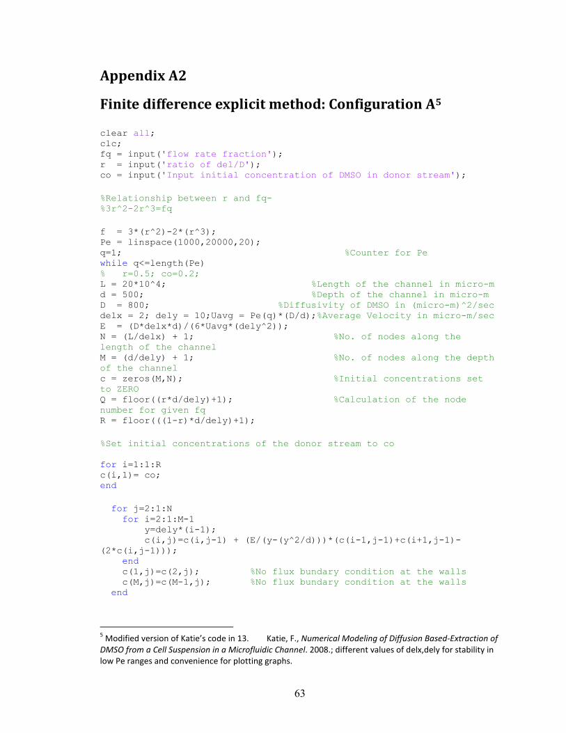
Finite difference explicit method: Configuration A5 clear all; clc; fq = input('flow rate fraction'); r = input('ratio of del/D'); co = input('Input initial concentration of DMSO in donor stream'); %Relationship between r and fq- %3r^2-2r^3=fq
f = 3*(r^2)-2*(r^3); Pe = linspace(1000,20000,20); q=1; %Counter for Pe while q<=length(Pe) % r=0.5; co=0.2; L = 20*10^4; %Length of the channel in micro-m d = 500; %Depth of the channel in micro-m D = 800; %Diffusivity of DMSO in (micro-m)^2/sec delx = 2; dely = 10;Uavg = Pe(q)*(D/d);%Average Velocity in micro-m/sec E = (D*delx*d)/(6*Uavg*(dely^2)); N = (L/delx) + 1; %No. of nodes along the length of the channel M = (d/dely) + 1; %No. of nodes along the depth of the channel c = zeros(M,N); %Initial concentrations set to ZERO Q = floor((r*d/dely)+1); %Calculation of the node number for given fq R = floor(((1-r)*d/dely)+1); %Set initial concentrations of the donor stream to co for i=1:1:R c(i,1)= co; end for j=2:1:N for i=2:1:M-1 y=dely*(i-1); c(i,j)=c(i,j-1) + (E/(y-(y^2/d)))*(c(i-1,j-1)+c(i+1,j-1)-(2*c(i,j-1))); end c(1,j)=c(2,j); %No flux bundary condition at the walls c(M,j)=c(M-1,j); %No flux bundary condition at the walls end
5 Modified version of Katie’s code in 13. Katie, F., Numerical Modeling of Diffusion Based-Extraction of
DMSO from a Cell Suspension in a Microfluidic Channel. 2008.; different values of delx,dely for stability in
low Pe ranges and convenience for plotting graphs.
64
%Average Outlet cell concentration for different Pe cell_sum(q) = sum(c(R+1:M,N)); donor_sum(q) = sum(c(1:R,N)); cell_avg(q) = cell_sum(q)/Q; donor_avg(q)= donor_sum(q)/R; overall_avg(q) = sum(c(1:M,N))/M; P(q) = L/(d*Pe(q)); %P = (1/Pe)*(L/d) q=q+1; end
int_limit = (1-fq)*(ones(1,length(Pe))); plot(P,cell_avg/co,'m'); P_cellavg = [P' (cell_avg/co)']; hold on; plot(P,int_limit,'--r'); hold on; P_donoravg = [P' (donor_avg/co)']; plot(P,donor_avg/co,'b'); xlabel('(1/Pe)*(L/d)'); ylabel('C/Co'); title('C/Co vs (1/Pe)*(L/d)');
65
Appendix A3
Finite difference implicit method: Configuration A %f - ratio delta/d %Pe -Peclet Number %Co - Initial Donor stream concentration % Repeat for different values of Pe f = input('ratio of del/D'); Co = input('Input initial concentration of DMSO in donor stream'); Pe = input('Peclet Number'); L = 23.2*10^4; % length in micro meters d = 500; % depth in micro-meters D = 800; % Diffusivity IMAX = 251; % No. of nodes along the depth direction dely = d/(IMAX-1); % delx = 5*dely; % lets assume delx JMAX = (L/(delx)) + 1; Uavg = Pe*(D/d); alpha = (delx*D)/((dely)^2); err = 1; j=1; R = floor(((1-f)*d/dely)+1); C = zeros(IMAX); for i=1:1:R %Set initial concentrations of the donor stream to co C(i)= Co; end for p=2:1:IMAX-1 y(p) = ((dely)*(p-1))/d ; u(p) = 6*Uavg *(y(p) - (y(p)^2)); beta(p) = alpha/(u(p)); end while j <= JMAX for q=1:1:IMAX-2 d(q) = -C(q+1); a(q) = beta(q+1); c(q) = beta(q+1); b(q) = -(1+ (2* beta(q+1))); end a(1) = 0; b(1) = beta(2)+b(1); b(IMAX-2) = b(1); c(IMAX-2) = 0; r = triDiagonal(a,b,c,d,IMAX-2); r = [r(1); r';r(IMAX-2)]; C = r; j=j+1;
66
end %Average Outlet cell concentration for different Pe cell_sum = sum(C(R+1:IMAX)); donor_sum = sum(C(1:R)); cell_avg = cell_sum/(IMAX-R); donor_avg = donor_sum/R; cell_avg_norm = cell_avg/Co; donor_avg_norm = donor_avg/Co;
Subfunction for solving Tridiagonal matrix
function u=triDiagonal(a,b,c,d,N) e = 1e-5; for k=2:1:N m = a(k)/b(k-1); b(k) = b(k) - m*c(k-1); d(k) = d(k) - m*d(k-1); if b(k) ==0 b(k) = b(k) + e; else u(k) = d(k)/b(k); end end for j=1:1:N-1 i=N-j; u(i) = (d(i)-(c(i)*u(i+1)))/(b(i)); end
67
Appendix B
Protocol for using the UV spectrophotometer for DMSO
concentration analysis
The following are the instructions for using the spectrophotometer for measuring
concentration of DMSO of the unknown sample. In general, I have used a 1/4th
dilution
scheme for the control as well as the unknown sample solution and 3 sets of wells in the
plate for each of the solution.
• Turn on spectrophotometer and allow the machine to calibrate. (Give it at least 15
minutes of warm-up time)
• Open Plate Reader software.
• Click the Setup button.
- Under options, click on Blanking. Uncheck Pre-Read Plate.
- Still in setup, under options, click wavelengths. Set desired wavelength, for DMSO