Introduction - Rowan Universityusers.rowan.edu/~hassen/Papers/distprime.pdf · Introduction This...

THE RIEMANN ZETA FUNCTION AND ITS APPLICATION TO NUMBER THEORY

ABDULKADIR HASSEN AND MARVIN KNOPP

1. Introduction

This paper is based on lecture notes given by the second author at Temple University in the spring of 1994.It was in these lectures that the first author was introduced to the theory of the Riemann zeta function. Weclaim no originality in this exposition. All results and proofs are due to others and our contribution here isthe selection of material and presentation. We hope that this paper will introduce young mathematicians tothis beautiful theory and inspire them to go beyond these pages!

The Riemann zeta function is defined by

ζ(s) =∞∑

n=1

1ns

, for σ > 1, (1)

where s = σ + it. The notation s for a complex number is due to Riemann and is now standard in thiscontext. In this article we discuss and prove some of the basic properties of ζ(s). Our main goal will be toshow how to apply the zeta function in the proof of the Prime Number Theorem, henceforth abbreviated byPNT.

Legendre and Gauss independently conjectured the PNT as follows. Let π(x) be the number of primesless than or equal to x, where x is a positive real number. Then

limx→∞

π(x)x

log x

= 1. (2)

In his only paper in number theory, in 1859, Riemann uncovered a deep relationship between the zerosof the zeta function and π(x). This eight-page paper in fact gave rise to what is now known as analyticnumber theory, a branch of number theory that uses complex analysis in tackling problems involving inte-gers. Based on the ideas of Riemann, Hadamard and de la Valle Poussin independently proved PNT in 1896.Both mathematicians used methods from complex analysis, establishing as a main step of the proof that theRiemann zeta function ζ(s) is nonzero for all complex values of the variable s that have the form s = 1 + itwith t > 0.

To expose this point of view is one of the intentions of this paper. We hope that the reader will becurious and interested enough to explore this rich and vibrant field of mathematics. For this we recommendthe introductory texts in this area, among which we mention Apostol [1], Chandrasekharan [4], Hardy andWright [6], Ireland and Rosen [8], Niven, Zuckerman and Montgomery [16], Patterson [17] and Rademacher[18].

Date: 7/18/07.2000 Mathematics Subject Classification. Primary 11M41.Key words and phrases. Riemann zeta function, functional equation, Prime Number Theorem, Theta function, Poisson

summation formula .

1

2 ABDULKADIR HASSEN AND MARVIN KNOPP

Section 2 will review the necessary background material needed to develop the theory of the Riemann zetafunction as it pertains to the proof of PNT. In section 3 we will develop the properties of the zeta function andprove the functional equation it satisfies. In section 4 we will first give some elementary theorems involvingπ(x) and conclude the section with D. J. Newman’s much simplified (and much admired) complex-variablesproof of PNT.

2. Preliminaries

Clearly the series defining ζ(s) in (1) convergence absolutely for σ > 1. However the most interestingproperties of zeta are observed in the region where σ ≤ 1. The series representation given by (1) is invalidin this region and therefore we have to find a way to extend it to this region. The most fruitful analyticcontinuation of zeta is by way of integration. Thus we will be defining functions using integrals and justifythat such functions are analytic. In many instances we need to interchange the processes of integration, limitand summation.

In order to keep our exposition brief and to focus on the important technical aspects of the application ofthe zeta function to PNT, we shall assume that the reader is familiar with the theory of the functions of onecomplex variable and convergence theorems of real analysis. One of the theorems of real analysis we will beusing often is the Weierstrass M-test for uniform convergence of series of functions. We will also be usingconsequences of uniform convergence. For readers with graduate level real analysis, we point out that theintegrals we deal with can be considered as Lebesgue integrals and thus we can easily appeal to the LebesgueDominated Convergence Theorem. For proofs of theorems related to these topics, we refer the reader to anystandard textbook of real and complex analysis but we mention Bak and Newman [2], Goldberg [5](Chapter9), Hijab [7], Knopp [9](Chapter XII, Sections 56 to 58), and Titchmarsh [21].

One of the most important theorems of complex analysis that we will be using frequently is the IdentityTheorem. Here is the statement of the theorem. For the proof we refer the reader to Marsden [13]( Page 397).

Theorem 1. Identity Theorem or The Principle of Analytic Continuation Let f and g be analyticin a region R. Suppose that there is a sequence {zn} of distinct points of R converging to a point z0 ∈ Rsuch that f(zn) = g(zn) for all n = 1, 2, 3, · · · . Then f = g on all of R.

Example: Let g(z) =∑∞

n=0 zn and f(z) = 11−z . If |z| < 1, g(z) = f(z).(The series is a geometric

series.) f(z) is analytic everywhere except at z = 1. Thus f is an analytic continuation of g in the sensethat we define g(z) to be f(z) for z 6= 1.

To obtain a different representation of the Riemann zeta function it is essential to use the gamma andtheta functions. We shall define these two functions next and state the main properties that we shall needfor our investigation of ζ.

Definition 1. The gamma function, denoted by Γ(s), is defined by

Γ(s) =∫ ∞

0

xs−1e−x dx, σ > 0.

Integration by parts (u = e−x, dv = xs−1dx) yields

Γ(s) =1sΓ(s + 1).

Note then that if s = n is a positive integer, then Γ(n) = (n − 1)!. More importantly, we note that theintegral defining Γ(s + 1) is convergent for Re(s) > −1 and hence 1

sΓ(s + 1) is the analytic continuation ofΓ(s) to the region Re(s) > −1. We repeat this process to extend Γ(s) to the whole plane with simple poles

THE RIEMANN ZETA FUNCTION AND ITS APPLICATION TO NUMBER THEORY 3

at the nonpositive integers. One of the classical books on special functions, Lebedev [12](Chapter 1), treatsmany interesting properties and applications of the gamma function.

Next we introduce the theta function.

Definition 2. The theta function Θ(z) is defined by

Θ(z) =∞∑

n=−∞en2πiz = 1 + 2

∞∑

n=1

en2πiz , Im(z) = y > 0.

The importance of the theta function lies in the property that we state in

Theorem 2. (The Transformation Law of Theta)(1) Θ(z + 2) = Θ(z).

(2) Θ(−1

z

)= e

−πi4 z

12 Θ(z).

As we shall see later, the transformation law stated above plays an important role in the analytic contin-uation of the zeta function. In fact, the functional equation of ζ(s) is a consequence of this transformationlaw. For the sake of simplicity we will proof a special case of Theorem 2 that we state in the followingproposition. However, we note that the Identity Theorem can easily be used to deduce Theorem 2 from

Proposition 1. If x > 0, then

Θ(

i

x

)= x

12 Θ(ix).

To prove this form of the transformation law of the theta function, we first need the following theoremfrom analysis.

Theorem 3. (Poisson Summation Formula) If f is continuous on the real line and∑∞

n=−∞ f(n + t)converges uniformly on 0 ≤ t ≤ 1 and if

∑∞n=−∞ f(n)e2πint converges, then

∞∑

n=−∞f(n + t) =

∞∑

n=−∞f (n)e2πint,

where

f (n) =∫ ∞

−∞f(x)e−2πinx dx.

Proof: Define φ(t) =∑∞

m=−∞ f(t + m). By our hypotheses, on the real line φ is continuous and clearlyφ(t + 1) = φ(t). Thus φ(t) has a Fourier series expansion given by

φ(t) =∞∑

n=−∞ane2πint,

where

an =∫ 1

0

φ(x)e−2πinx dx.

That the Fourier series for φ(x) is equal to the function follows from the fact that φ(t) is uniformly continuouson [0, 1] and that the Fourier series is uniformly convergent in [0, 1]. (For a detailed proof of this see [21],


page 414. See also [10], page 39.) Let us find an by substituting the summation for φ(x) in the integral.(We leave it to the reader to justify the permissibility of interchanging summation and integration.)

an =∫ 1

0

φ(x)e−2πinx dx =∫ 1

0

∞∑

m=−∞f(x + m)e−2πinx dx

=∞∑

m=−∞

∫ 1

0

f(x + m)e−2πinx dx =∞∑

m=−∞

∫ m+1

m

f(x)e−2πinx dx

=∫ ∞

−∞f(x)e−2πinx dx = f(n),

as desired.

Proof of Proposition 1: In what follows x is a fixed positive real number. We shall write exp(z)instead of ez whenever it is convienient. Again we leave it to the reader to justify interchanging summationsand integration.

Define f(u) = e−πu2x. Then∑∞

n=−∞ f(n) =∑∞

n=−∞ e−πn2x converges and by the Poisson SummationFormula (with t = 0), we have

Θ(ix) =∞∑

n=−∞f(n) =

∞∑

n=−∞f (n) =

∞∑

n=−∞

∫ ∞

−∞f(u)e−2πinu du. (3)

But f(u) = exp(−u2x

)and hence by completing the square we have

exp(−πu2x − 2πinu

)= exp

(−πx

(u2 + 2inu/x

))= exp

(−πx (u + in/x)2 − πn2/x

).

The change of variable t = u + in/x then yields∫ ∞

−∞f(u)e−2πinu du =

∫ ∞

−∞exp

(−πx (u + in/x)2 − πn2/x

)du = e−πn2/x

∫ ∞+in/x

−∞+in/x

exp(−πxt2

)dt.

It can be shown that∫ ∞+ in

x

−∞+ inx

exp(−πxt2

)dt =

∫ ∞

−∞exp

(−πxt2

)dt. (4)

Thus we have ∫ ∞

−∞f(u)e exp (−2πinu) du = exp

(−

πn2

x

)∫ ∞

−∞exp

(−πxt2

)dt.

Finally to remove x form the integral, we let t = y/√

πx. This yields

∫ ∞

−∞f(u) exp (−2πinu) du =

exp(−πn2

x

)

√πx

∫ ∞

−∞exp

(−y2

)dy = γ

exp(−πn2

x

)

√x

, (5)

where

γ =1√π

∫ ∞

−∞e−y2

dy.

Substituting (5) in (3) and noting that γ is a constant, we obtain

Θ(ix) =γ√x

Θ(

i

x

). (6)


To complete the proof wee need to show γ = 1. Since (6) holds for all x > 0, putting x = 1 in the equationyields γ = 1, thereby completing the proof of the proposition.

As a consequence of Proposition 1, we have the following

Corollary 1. For t > 0, let Ψ(t) =∑∞

n=1 e−πn2x. Then

Ψ(

1t

)= −1

2+

12t1/2 + t1/2Ψ(t). (7)

Proof: This follows from the fact that Ψ(t) = Θ(it)−12 .

3. The Riemann Zeta Function

Recall that the Riemann zeta function is defined by

ζ(s) =∞∑

n=1

1ns

, for σ > 1,

where s = σ + it. Since |n−s| = n−σ, it follows from the integral test for convergence of infinite series thatthe series converges absolutely for σ > 1. Furthermore, if a > 1 and σ ≥ a, then

∞∑

n=1

∣∣∣∣1ns

∣∣∣∣ =∞∑

n=1

1nσ

≤∞∑

n=1

1na

< ∞.

Thus convergence is uniform for σ > a, and therefore ζ(s) is analytic in the region σ > 1. For an in-depthanalysis and detailed proofs of properties of the Riemann zeta function, we recommend Titchmarsh [20].

Theorem 4. ζ(s) can be extended meromorphically to the right half-plane σ > 0 and, in fact, ζ(s) − 1s−1 is

analytic in σ > 0.

Poof: For σ > 0, define

φn(s) =1ns

−∫ n+1

n

1us

du =∫ n+1

n

(1ns

− 1us

)du.

Then

|φn(s)| =∣∣∣∣∫ n+1

n

(1ns

−1us

)du

∣∣∣∣ ≤ maxu∈[n,n+1]

(n−s − u−s

).

But n−s − u−s =∫ u

nsx−s−1 dx. Thus we have

∣∣n−s − u−s∣∣ ≤ |s|

∫ n+1

n

x−σ−1 dx ≤ |s|σ

(n−σ − (n + 1)−σ

).

Adding over n we get∞∑

n=1

|φn(s)| ≤|s|σ

∞∑

n=1

(n−σ − (n + 1)−σ

)=

|s|σ

.

Thus∑∞

n=1 φn(s) converges absolutely and uniformly in σ > a, a > 0. Since φn(s) is entire, it follows thatthe function F (s) defined by

F (s) =∞∑

n=1

φn(s)


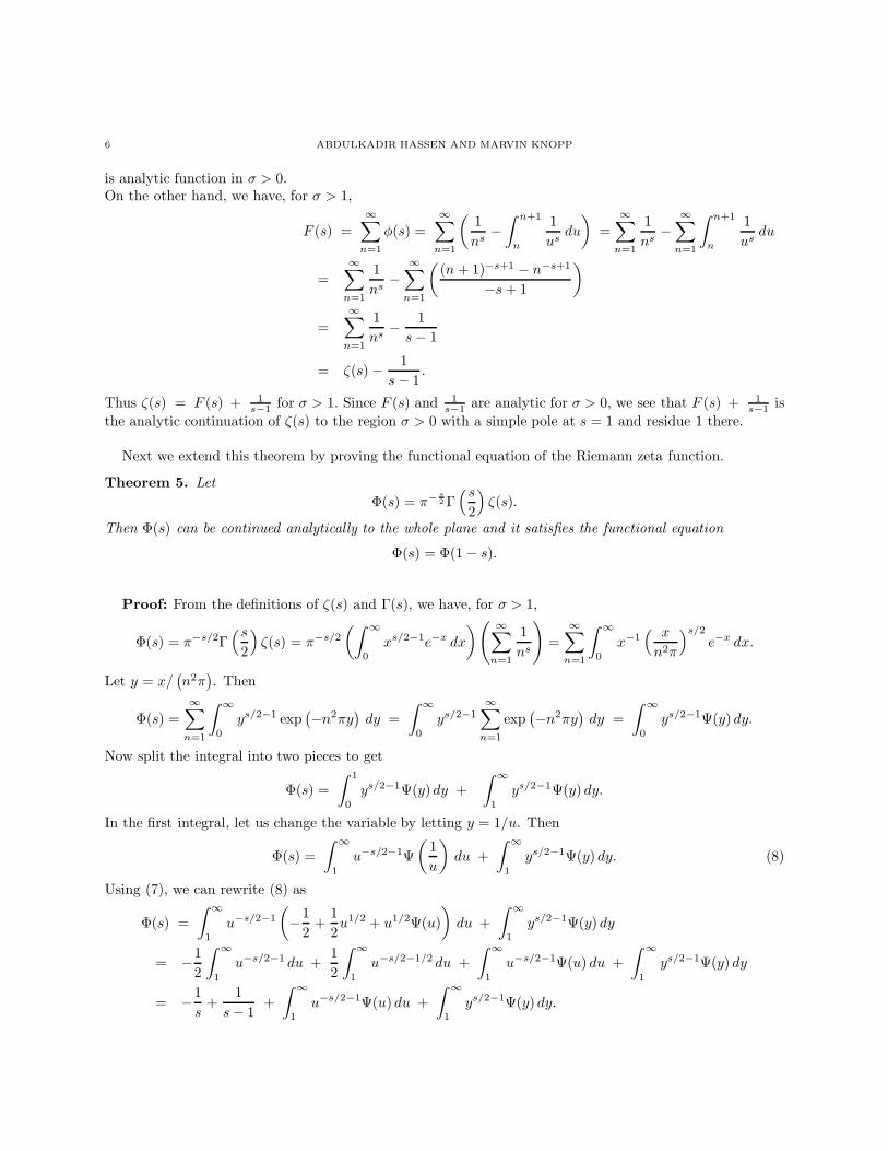
is analytic function in σ > 0.On the other hand, we have, for σ > 1,

F (s) =∞∑

n=1

φ(s) =∞∑

n=1

(1ns

−∫ n+1

n

1us

du

)=

∞∑

n=1

1ns

−∞∑

n=1

∫ n+1

n

1us

du

=∞∑

n=1

1ns

−∞∑

n=1

((n + 1)−s+1 − n−s+1

−s + 1

)

=∞∑

n=1

1ns

− 1s − 1

= ζ(s) − 1s − 1

.

Thus ζ(s) = F (s) + 1s−1 for σ > 1. Since F (s) and 1

s−1 are analytic for σ > 0, we see that F (s) + 1s−1 is

the analytic continuation of ζ(s) to the region σ > 0 with a simple pole at s = 1 and residue 1 there.

Next we extend this theorem by proving the functional equation of the Riemann zeta function.

Theorem 5. LetΦ(s) = π− s

2 Γ(s

2

)ζ(s).

Then Φ(s) can be continued analytically to the whole plane and it satisfies the functional equation

Φ(s) = Φ(1 − s).

Proof: From the definitions of ζ(s) and Γ(s), we have, for σ > 1,

Φ(s) = π−s/2Γ(s

2

)ζ(s) = π−s/2

(∫ ∞

0

xs/2−1e−x dx

)( ∞∑

n=1

1ns

)=

∞∑

n=1

∫ ∞

0

x−1( x

n2π

)s/2

e−x dx.

Let y = x/(n2π

). Then

Φ(s) =∞∑

n=1

∫ ∞

0

ys/2−1 exp(−n2πy

)dy =

∫ ∞

0

ys/2−1∞∑

n=1

exp(−n2πy

)dy =

∫ ∞

0

ys/2−1Ψ(y) dy.

Now split the integral into two pieces to get

Φ(s) =∫ 1

0

ys/2−1Ψ(y) dy +∫ ∞

1

ys/2−1Ψ(y) dy.

In the first integral, let us change the variable by letting y = 1/u. Then

Φ(s) =∫ ∞

1

u−s/2−1Ψ(

1u

)du +

∫ ∞

1

ys/2−1Ψ(y) dy. (8)

Using (7), we can rewrite (8) as

Φ(s) =∫ ∞

1

u−s/2−1

(−1

2+

12u1/2 + u1/2Ψ(u)

)du +

∫ ∞

1

ys/2−1Ψ(y) dy

= −12

∫ ∞

1

u−s/2−1 du +12

∫ ∞

1

u−s/2−1/2 du +∫ ∞

1

u−s/2−1Ψ(u) du +∫ ∞

1

ys/2−1Ψ(y) dy

= −1s

+1

s − 1+∫ ∞

1

u−s/2−1Ψ(u) du +∫ ∞

1

ys/2−1Ψ(y) dy.


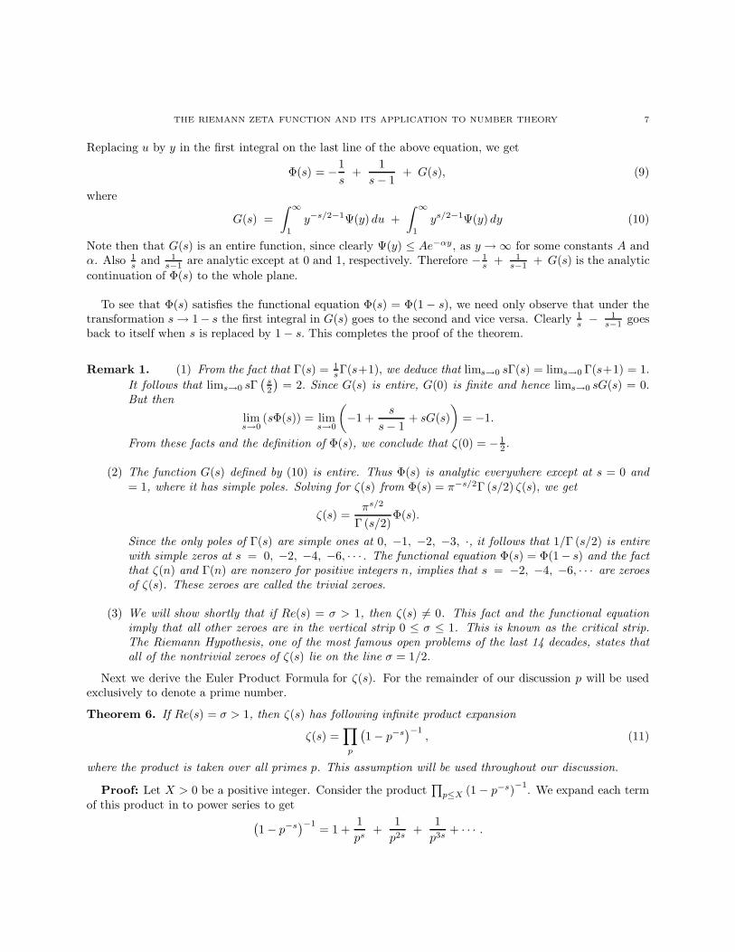
Replacing u by y in the first integral on the last line of the above equation, we get

Φ(s) = −1s

+1

s − 1+ G(s), (9)

where

G(s) =∫ ∞

1

y−s/2−1Ψ(y) du +∫ ∞

1

ys/2−1Ψ(y) dy (10)

Note then that G(s) is an entire function, since clearly Ψ(y) ≤ Ae−αy, as y → ∞ for some constants A andα. Also 1

s and 1s−1 are analytic except at 0 and 1, respectively. Therefore −1

s + 1s−1 + G(s) is the analytic

continuation of Φ(s) to the whole plane.

To see that Φ(s) satisfies the functional equation Φ(s) = Φ(1 − s), we need only observe that under thetransformation s → 1− s the first integral in G(s) goes to the second and vice versa. Clearly 1

s − 1s−1 goes

back to itself when s is replaced by 1 − s. This completes the proof of the theorem.

Remark 1. (1) From the fact that Γ(s) = 1sΓ(s+1), we deduce that lims→0 sΓ(s) = lims→0 Γ(s+1) = 1.

It follows that lims→0 sΓ(

s2

)= 2. Since G(s) is entire, G(0) is finite and hence lims→0 sG(s) = 0.

But then

lims→0

(sΦ(s)) = lims→0

(−1 +

s

s − 1+ sG(s)

)= −1.

From these facts and the definition of Φ(s), we conclude that ζ(0) = −12 .

(2) The function G(s) defined by (10) is entire. Thus Φ(s) is analytic everywhere except at s = 0 and= 1, where it has simple poles. Solving for ζ(s) from Φ(s) = π−s/2Γ (s/2) ζ(s), we get

ζ(s) =πs/2

Γ (s/2)Φ(s).

Since the only poles of Γ(s) are simple ones at 0, −1, −2, −3, ·, it follows that 1/Γ (s/2) is entirewith simple zeros at s = 0, −2, −4, −6, · · · . The functional equation Φ(s) = Φ(1− s) and the factthat ζ(n) and Γ(n) are nonzero for positive integers n, implies that s = −2, −4, −6, · · · are zeroesof ζ(s). These zeroes are called the trivial zeroes.

(3) We will show shortly that if Re(s) = σ > 1, then ζ(s) 6= 0. This fact and the functional equationimply that all other zeroes are in the vertical strip 0 ≤ σ ≤ 1. This is known as the critical strip.The Riemann Hypothesis, one of the most famous open problems of the last 14 decades, states thatall of the nontrivial zeroes of ζ(s) lie on the line σ = 1/2.

Next we derive the Euler Product Formula for ζ(s). For the remainder of our discussion p will be usedexclusively to denote a prime number.

Theorem 6. If Re(s) = σ > 1, then ζ(s) has following infinite product expansion

ζ(s) =∏

p

(1 − p−s

)−1, (11)

where the product is taken over all primes p. This assumption will be used throughout our discussion.

Proof: Let X > 0 be a positive integer. Consider the product∏

p≤X (1 − p−s)−1. We expand each termof this product in to power series to get

(1 − p−s

)−1 = 1 +1ps

+1

p2s+

1p3s

+ · · · .


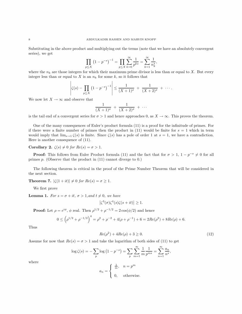
Substituting in the above product and multiplying out the terms (note that we have an absolutely convergentseries), we get

∏

p≤X

(1 − p−s

)−1 =∏

p≤X

∞∑

k=0

1pks

=∞∑

k=1

1ns

k

,

where the nk are those integers for which their maximum prime divisor is less than or equal to X. But everyinteger less than or equal to X is an nk for some k, so it follows that

∣∣∣∣∣∣ζ(s) −

∏

p≤X

(1 − p−s

)−1

∣∣∣∣∣∣≤ 1

(X + 1)σ+

1(X + 2)σ

+ · · · .

We now let X → ∞ and observe that1

(X + 1)σ+

1(X + 2)σ

+ · · ·

is the tail end of a convergent series for σ > 1 and hence approaches 0, as X → ∞. This proves the theorem.

One of the many consequences of Euler’s product formula (11) is a proof for the infinitude of primes. Forif there were a finite number of primes then the product in (11) would be finite for s = 1 which in termwould imply that lims→1 ζ(s) is finite. Since ζ(s) has a pole of order 1 at s = 1, we have a contradiction.Here is another consequence of (11).

Corollary 2. ζ(s) 6= 0 for Re(s) = σ > 1.

Proof: This follows from Euler Product formula (11) and the fact that for σ > 1, 1 − p−s 6= 0 for allprimes p. (Observe that the product in (11) cannot diverge to 0.)

The following theorem is critical in the proof of the Prime Number Theorem that will be considered inthe next section.

Theorem 7. |ζ(1 + it)| 6= 0 for Re(s) = σ ≥ 1.

We first prove

Lemma 1. For s = σ + it, σ > 1,and t 6= 0, we have∣∣ζ3(σ)ζ4(s)ζ(s + it)

∣∣ ≥ 1.

Proof: Let ρ = eiφ, φ real. Then ρ1/2 + ρ−1/2 = 2 cos(φ/2) and hence

0 ≤(ρ1/2 + ρ−1/2

)4

= ρ2 + ρ−2 + 4(ρ + ρ−1) + 6 = 2Re(ρ2) + 8Re(ρ) + 6.

Thus

Re(ρ2) + 4Re(ρ) + 3 ≥ 0. (12)

Assume for now that Re(s) = σ > 1 and take the logarithm of both sides of (11) to get

log ζ(s) = −∑

p

log(1 − p−s

)=∑

p

∞∑

m=1

1m

1pms

=∞∑

n=1

an

ns,

where

an =

1m , n = pm

0, otherwise.


Here we have applied the power series expansion of log(1−x) and rearranged the double sum. From this weconclude that

log ζ(σ) =∞∑

n=1

ann−σ, log ζ(s) =∞∑

n=1

(ann−σ

)n−it, log ζ(s + it) =

∞∑

n=1

(ann−σ

)n−2it.

Note that ann−σ ≥ 0. Put ρ = n−it = e−it log n. Then |ρ| = 1 and by (12) we have

Re(n−2it) + 4Re(n−it) + 3 ≥ 0.

Multiplying this inequality by ann−σ ≥ 0, noting the fact that Re(ann−σn−it

)= (ann−σ)Re

(n−it

), and

adding the resulting inequality over n, we get∞∑

n=1

{Re(ann−σn−2it

)+ 4Re

(ann−σn−it

)+ 3ann−σ

}≥ 0.

Thus we haveRe(log ζ(σ + 2it) + 4 log ζ(s) + 3 log ζ(σ)

)≥ 0

and exponentiation yields

exp(Re(log ζ(σ + 2it) + 4 log ζ(s) + 3 log ζ(σ)

))≥ 1.

This implies thatexp (Re(log ζ(σ + 2it)) · exp (4 log ζ(s)) · exp (3 log ζ(σ))) ≥ 1.

Since |z| = exp(Re(log(z)

))holds for all z, we conclude that

∣∣ζ3(σ)ζ4(s)ζ(s + it)∣∣ ≥ 1,

as desired.

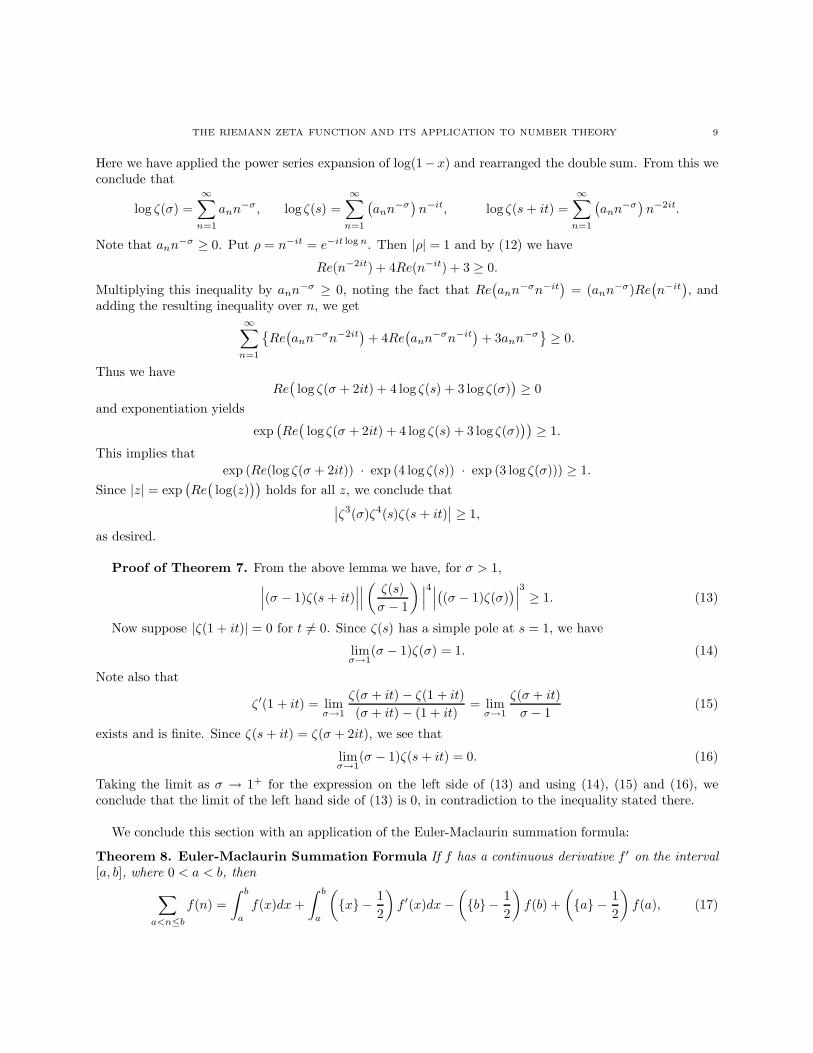
Proof of Theorem 7. From the above lemma we have, for σ > 1,∣∣∣(σ − 1)ζ(s + it)

∣∣∣∣∣∣(

ζ(s)σ − 1

)∣∣∣4∣∣∣((σ − 1)ζ(σ)

)∣∣∣3

≥ 1. (13)

Now suppose |ζ(1 + it)| = 0 for t 6= 0. Since ζ(s) has a simple pole at s = 1, we have

limσ→1

(σ − 1)ζ(σ) = 1. (14)

Note also that

ζ′(1 + it) = limσ→1

ζ(σ + it) − ζ(1 + it)(σ + it) − (1 + it)

= limσ→1

ζ(σ + it)σ − 1

(15)

exists and is finite. Since ζ(s + it) = ζ(σ + 2it), we see that

limσ→1

(σ − 1)ζ(s + it) = 0. (16)

Taking the limit as σ → 1+ for the expression on the left side of (13) and using (14), (15) and (16), weconclude that the limit of the left hand side of (13) is 0, in contradiction to the inequality stated there.

We conclude this section with an application of the Euler-Maclaurin summation formula:

Theorem 8. Euler-Maclaurin Summation Formula If f has a continuous derivative f ′ on the interval[a, b], where 0 < a < b, then

∑

a<n≤b

f(n) =∫ b

a

f(x)dx +∫ b

a

({x} − 1

2

)f ′(x)dx −

({b} − 1

2

)f(b) +

({a} − 1

2

)f(a), (17)


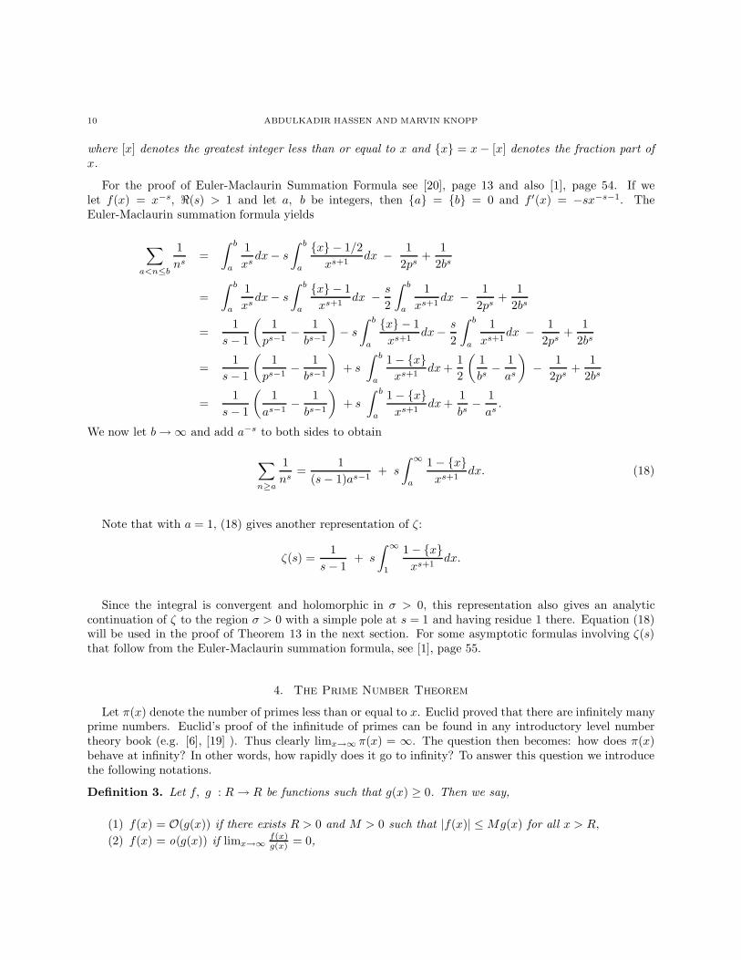
where [x] denotes the greatest integer less than or equal to x and {x} = x − [x] denotes the fraction part ofx.

For the proof of Euler-Maclaurin Summation Formula see [20], page 13 and also [1], page 54. If welet f(x) = x−s, <(s) > 1 and let a, b be integers, then {a} = {b} = 0 and f ′(x) = −sx−s−1. TheEuler-Maclaurin summation formula yields

∑

a<n≤b

1ns

=∫ b

a

1xs

dx− s

∫ b

a

{x} − 1/2xs+1

dx − 12ps

+1

2bs

=∫ b

a

1xs

dx− s

∫ b

a

{x} − 1xs+1

dx −s

2

∫ b

a

1xs+1

dx −1

2ps+

12bs

=1

s − 1

(1

ps−1− 1

bs−1

)− s

∫ b

a

{x} − 1xs+1

dx− s

2

∫ b

a

1xs+1

dx − 12ps

+1

2bs

=1

s − 1

(1

ps−1− 1

bs−1

)+ s

∫ b

a

1 − {x}xs+1

dx +12

(1bs

− 1as

)− 1

2ps+

12bs

=1

s − 1

(1

as−1− 1

bs−1

)+ s

∫ b

a

1 − {x}xs+1

dx +1bs

− 1as

.

We now let b → ∞ and add a−s to both sides to obtain

∑

n≥a

1ns

=1

(s − 1)as−1+ s

∫ ∞

a

1 − {x}xs+1

dx. (18)

Note that with a = 1, (18) gives another representation of ζ:

ζ(s) =1

s − 1+ s

∫ ∞

1

1 − {x}xs+1

dx.

Since the integral is convergent and holomorphic in σ > 0, this representation also gives an analyticcontinuation of ζ to the region σ > 0 with a simple pole at s = 1 and having residue 1 there. Equation (18)will be used in the proof of Theorem 13 in the next section. For some asymptotic formulas involving ζ(s)that follow from the Euler-Maclaurin summation formula, see [1], page 55.

4. The Prime Number Theorem

Let π(x) denote the number of primes less than or equal to x. Euclid proved that there are infinitely manyprime numbers. Euclid’s proof of the infinitude of primes can be found in any introductory level numbertheory book (e.g. [6], [19] ). Thus clearly limx→∞ π(x) = ∞. The question then becomes: how does π(x)behave at infinity? In other words, how rapidly does it go to infinity? To answer this question we introducethe following notations.

Definition 3. Let f, g : R → R be functions such that g(x) ≥ 0. Then we say,

(1) f(x) = O(g(x)) if there exists R > 0 and M > 0 such that |f(x)| ≤ Mg(x) for all x > R,

(2) f(x) = o(g(x)) if limx→∞f(x)g(x) = 0,


(3) f(x) ∼ g(x) if limx→∞f(x)g(x)

= 1.

If f and g satisfy definition 3, we say that they are asymptotic. The following facts can easily be provedand will be used freely.

(1) O(O (g(x))) = O(g(x)),(2) O(g(x)) ± O(g(x)) = O(g(x)),(3) O(g(x)) ± o(g(x)) = O(g(x)),(4) (O (g(x)))2 = O

((g(x))2

).

Theorem 9. (The Prime Number Theorem - PNT)

limx→∞

π(x)(x

log x

) = 1. (19)

The proof of PNT is one of the crowning achievements of modern mathematics. The effort made inproving it had tremendous impact upon the development of complex analysis in the 19th and 20th centuries.Among the principal contributers to the proof of the PNT were Legendre, Gauss, Tchebychev, Riemann,Dirichlet, Hadamard, and De la Valle Poussin. Each of these mathematicians used the methods of analysis.In 1949 Erdos and Selberg gave a proof that is elementary in the sense that it does not use the methods ofanalysis. For a brief summary of the history of the theorem and its impact see the excellent and readablepaper of Bateman and Diamond [3]. The first proof of the theorem appeared in 1896, given independentlyby Hadamard and De la Valle Poussin. In this section we present the proof of Newman [14] (See also [15],Chapter 7).

In 1796, Adrien-Marie Legendre conjectured that

π(x) ∼ x

logx − B, (20)

where B=1.08... is a certain constant close to 1.

Carl Friedrich Gauss, based on the computational evidence available to him and on some heuristic rea-soning, was able to arrive at his own approximating function. We state Guass’s conjecture as follows.

If we define

Li(x) =∫ x

3

dt

log t, (21)

then

π(x) ∼ Li(x). (22)

One can show that Li(x) has the following expansion.

Li(x) =x

logx+

x

(log x)2+

2!x(log x)3

+3!x

(logx)4+ · · · +

n!x(log x)n+1 (1 + ε(x)) , (23)

where ε(x) → 0 as x → ∞.

The Russian mathematician Pafnuty L’vovich Tchebyshev attempted to prove PNT in two papers from1848 and 1850. In fact, Tchebychev proved the following two statements about distribution of primes. Notethat these statements are weaker than PNT.


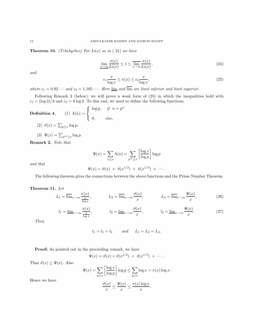
Theorem 10. (Tchebychev) For Li(x) as in ( 21) we have

limx→∞

π(x)Li(x)

≤ 1 ≤ limx→∞

π(x)Li(x)

, (24)

and

c1x

logx≤ π(x) ≤ c2

x

log x, (25)

where c1 = 0.92 · · · and c2 = 1.105 · · ·. Here lim and lim are limit inferior and limit superior.

Following Remark 3 (below), we will prove a weak form of (25) in which the inequalities hold withc1 = (log 2)/3 and c2 = 8 log2. To this end, we need to define the following functions.

Definition 4. (1) Λ(n) =

log p, if n = pα

0, else,

(2) ϑ(x) =∑

p≤x log p,

(3) Ψ(x) =∑

pm≤x log p.

Remark 2. Note that

Ψ(x) =∑

n≤x

Λ(n) =∑

pm≤x

[log x

log p

]logp

and thatΨ(x) = ϑ(x) + ϑ(x1/2) + ϑ(x1/3) + · · · .

The following theorem gives the connections between the above functions and the Prime Number Theorem.

Theorem 11. Let

L1 = limx→∞π(x)

xlogx

, L2 = limx→∞ϑ(x)

x, L3 = limx→∞

Ψ(x)x

, (26)

l1 = limx→∞π(x)

xlog x

, l2 = limx→∞ϑ(x)

x, l3 = limx→∞

Ψ(x)x

. (27)

Then

l1 = l2 = l3 and L1 = L2 = L3.

Proof: As pointed out in the preceeding remark, we have

Ψ(x) = ϑ(x) + ϑ(x1/2) + ϑ(x1/3) + · · · .

Thus ϑ(x) ≤ Ψ(x). Also

Ψ(x) =∑

p≤x

[log x

log p

]log p ≤

∑

p≤x

logx = π(x) log x.

Hence we haveϑ(x)

x≤ Ψ(x)

x≤ π(x) logx

x.


Taking lim sup we get L2 ≤ L3 ≤ L1. To complete the proof of L1 = L2 = L3, it suffices to show L2 ≥ L1.To this end, let 0 < α < 1 and x > 1. Then

ϑ(x) ≥∑

xα<p≤x

log p ≥ α logx∑

xα<p≤x

1 = α log x (π(x) − π(xα)) ≥ α log x (π(x) − xα) ,

since π(xα) ≤ xα. Thus we haveϑ(x)

x≥ α

π(x) logx

x− α

log x

x1−α.

Since limx→∞logxx1−α = 0, we conclude that

limx→∞ϑ(x)

x≥ αlimx→∞

π(x)x

logx

.

Thus L2 ≥ αL1 and taking the limit as α → 1−, we conclude that L2 ≥ L1.

Similar arguments can be used to show l1 = l2 = l3 and we leave this to the read as an exercise.

Remark 3. In view of the above theorem, note that PNT follows if we can show that l2 = L2 = 1. Themain goal of the remainder of this paper is to prove this fact.

We now prove a weaker form of ( 25) mentioned above. To this end, for any positive integer n, let

N =(

2nn

)=

(2n)!n!n!

=(n + 1)(n + 2) · · ·2n

1 · 2 · · ·n.

Then

22n = (1 + 1)2n =2n∑

k=0

(2nk

)>

(2nn

)= N.

Since(

2nk

)≤(

2nn

)for each k, we also have

22n = (1 + 1)2n =2n∑

k=0

(2nk

)≤

2n∑

k=0

(2nn

)= N (2n + 1).

We note thatN

2=

12

(2nn

)=

(2n)!(n!)2

n

2n=

(2n − 1)!n!(n− 1)!

=(

2n − 1n − 1

)

Thus N/2 is divisible by every prime in the range n < p ≤ 2n − 1 and hence divisible by their product. Inparticular, we have ∏

n<p≤2n

p ≤ N.

Combining the preceeding inequalities, we have proved∏

n<p≤2n

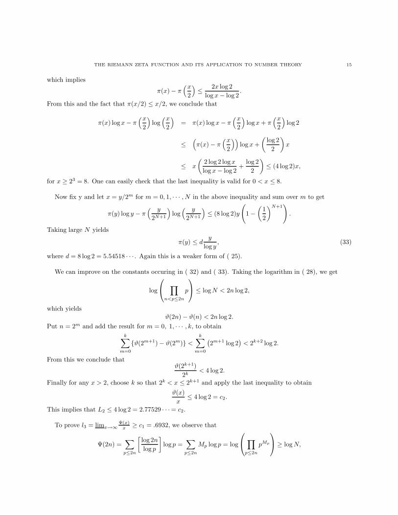
p ≤ N < 22n ≤ N (2n + 1). (28)

We also note that∏

n<p≤2n

p ≥∏

n<p≤2n

n = nπ(2n)−π(n) and 2n ≤n∏

k=1

k + n

k=

(n + 1)(n + 2) · · ·2n

1 · 2 · · ·n= N. (29)


On the other hand, if pα is the largest power of a prime p that divides n!, then

α =∞∑

m=1

[n

pm

].

(For the proof of this, see [1], page 67.) Since N = (2n)!n!n! , any prime that divides N must divide (2n)! and

hence is less than 2n. Thus if we writeN =

∏

p≤2n

pα(p),

then

α(p) =∞∑

m=1

([2n

pm

]− 2

[n

pm

]).

Note that pm > 2n (and hence[

2npm

]= 0) if and only if m > (log 2n)/ logp. Thus the above sum contains

no more than[

log 2nlogp

]terms. Also each term is either 0 or 1. Hence α(p) ≤

[log 2nlog p

]≤ log 2n

log p . But then

pα(p) ≤ 2n and we have proved that

N ≤ (2n)π(2n). (30)

From ( 28), ( 29) and ( 30) we get

2n ≤ (2n)π(2n) and nπ(2n)−π(n) ≤ 22n. (31)

Taking the logarithm of the first inequality in ( 31) yields

n log 2 ≤ π(2n) · log(2n).

For any real x ≥ 3, let n = [x/2]. Then n ≤ x/2 < n + 1 and hencex

2log 2 ≤ (n + 1) log2 = n log 2 + log 2 ≤ π(2n) log(2n) + log 2 ≤ π(x) log(x) + log 2 ≤ 3

2π(x) log x,

since 2 log2 ≤ π(x) log x for all x ≥ 3. Thus

c · x

logx≤ π(x) (32)

for any x ≥ 3 and c = (log2)/3 = 0.231049 · · · . This is much weaker than ( 25).

Taking the logarithm of the second inequality in ( 31) and dividing the resulting inequality by logn, weget

π(2n) − π(n) ≤ 2n

logn· log 2.

Now let x ≥ 6 be any real number, and let n = [x/2]. Then π(x/2) = π(n) and π(x) ≤ π(2n) + 1. Thus

π(x) − π(x/2) ≤ π(2n) − π(n) + 1 ≤2n

lognlog 2 + 1 =

2n log 2 + log n

logn≤

x log 2 + log(x/2)log(x/2 − 1)

.

For x ≥ 6, it can be shown thatx log 2 + log(x/2)

log(x/2 − 1)≤ 2x log 2

log(x/2).

We use this in the above inequality to conclude that(π(x) − π

(x

2

))log(x

2

)≤ 2x log 2,


which implies

π(x) − π(x

2

)≤ 2x log 2

log x − log 2.

From this and the fact that π(x/2) ≤ x/2, we conclude that

π(x) logx − π(x

2

)log(x

2

)= π(x) log x − π

(x

2

)logx + π

(x

2

)log 2

≤(π(x) − π

(x

2

))log x +

(log 2

2

)x

≤ x

(2 log2 logx

log x − log 2+

log 22

)≤ (4 log2)x,

for x ≥ 23 = 8. One can easily check that the last inequality is valid for 0 < x ≤ 8.

Now fix y and let x = y/2m for m = 0, 1, · · · , N in the above inequality and sum over m to get

π(y) log y − π( y

2N+1

)log( y

2N+1

)≤ (8 log 2)y

(1 −

(12

)N+1)

.

Taking large N yields

π(y) ≤ dy

logy, (33)

where d = 8 log2 = 5.54518 · · · . Again this is a weaker form of ( 25).

We can improve on the constants occuring in ( 32) and ( 33). Taking the logarithm in ( 28), we get

log

∏

n<p≤2n

p

≤ logN < 2n log 2,

which yieldsϑ(2n) − ϑ(n) < 2n log 2.

Put n = 2m and add the result for m = 0, 1, · · · , k, to obtaink∑

m=0

{ϑ(2m+1) − ϑ(2m)} <

k∑

m=0

(2m+1 log 2

)< 2k+2 log 2.

From this we conclude thatϑ(2k+1)

2k< 4 log 2.

Finally for any x > 2, choose k so that 2k < x ≤ 2k+1 and apply the last inequality to obtainϑ(x)

x≤ 4 log2 = c2.

This implies that L2 ≤ 4 log2 = 2.77529 · · ·= c2.

To prove l3 = limx→∞Ψ(x)

x ≥ c1 = .6932, we observe that

Ψ(2n) =∑

p≤2n

[log 2n

log p

]logp =

∑

p≤2n

Mp logp = log

∏

p≤2n

pMp

≥ log N,


where Mp = [ log 2nlog p ]. On the other hand, 22n ≤ (2n + 1)N implies N ≥ 22n

2n+1 and hence

logN ≥ 2n log 2 − log(2n + 1).

Therefore we haveΨ(2n) ≥ log N ≥ 2n log 2 − log(2n + 1).

For x > 2, let n =[

x2

]. Then n ≥ 1, n > x

2 − 1, and 2n ≤ x. Hence

Ψ(x) ≥ Ψ(2n) ≥ 2n log 2 − log(2n + 1) ≥ 2(x

2− 1) log2 − log(x + 1) = (x − 2) log2 − log(x + 1),

and dividing the first and last terms by x, we obtainΨ(x)

x≥ (x − 2) log2

x− log(x + 1)

x.

Taking lim inf and noting that limx→∞log(x+1)

x= 0, we conclude that

l3 ≥ log 2 = .6932 · · · ,

as desired.

We now return to the proof of limx→∞ϑ(x)

x = 1. We first prove the following theorem.

Theorem 12. Let

ρ(x) =∑

p≤x

log p

p. (34)

Then the following statements are equivalent.

(1) limx→∞ϑ(x)

x = 1.

(2) limx→∞ (ρ(x) − log x) exists.

Proof: We will show (2) ⇒ (1). Note that this is enough for our main objective here. We leave it to thereader to prove (1) ⇒ (2).

Let E = limx→∞

(ρ(x) − log x

). We observe that

n {ρ(n) − ρ(n − 1)} =

log p, if n = p

0, else,

and hence we have

ϑ(x) =∑

p≤x

log p

=∑

2≤n≤x

{ρ(n) − ρ(n − 1)

}n

=∑

2≤n≤x

{(ρ(n) − log n

)−(ρ(n − 1) − log(n − 1)

)}n +

∑

2≤n≤x

n log(

n

n − 1

).

Let

F1(x) =∑

2≤n≤x

{(ρ(n) − log n

)−(

ρ(n − 1) − log(n − 1))}

n,


and

F2(x) =∑

2≤n≤x

n log(

n

n − 1

).

ClaimF1(x) = o(x) and F2(x) = x + O(log x).

Note then thatϑ(x) = F1(x) + F2(x) = o(x) + x + O(log x) = x + o(x)

and hence

limx→∞

ϑ(x)x

= 1.

To prove the claim, we rewrite F1 as

F1(x) =∑

2≤n≤x

n{ρ(n) − logn

}−∑

2≤n≤x

n{

ρ(n − 1) − log(n − 1)}

=∑

2≤n≤x

n{ρ(n) − logn

}−

∑

1≤n≤x−1

(n + 1){ρ(n) − log(n)

}

=(ρ([x]) − log([x])

)[x] +

∑

2≤n≤x−1

n{

ρ(n) − log n}

−∑

1≤n≤x−1

n{

ρ(n) − log(n)}−

∑

1≤n≤x−1

{ρ(n) − log(n)

}

=(ρ([x]) − log([x])

)([x] + 1

)−∑

1≤n≤x

{ρ(n) − log(n)

}.

Let δ(x) = ρ(x) − logx − E. Then by assumption, limx→∞ δ(x) = 0. That is δ(x) = o(1) and we have

F1(x) =(δ([x]) + E

)([x] + 1

)−∑

1≤n≤x

(δ(n) + E

)

=(δ([x]) + E

)([x] + 1

)− [x] ·E −

∑

1≤n≤x

δ(n)

= E + δ([x])([x] + 1

)−∑

1≤n≤x

δ(n).

But ∑

1≤n≤x

δ(n) = o(x) and δ([x]) ([x] + 1) = o(x).

Therefore,F1(x) = E + o(x) = o(x).

Also

F2(x) =∑

2≤n≤x

n log(

n

n − 1

)=

∑

2≤n≤x

n log(

1 +1

n − 1

)

= 2 log2 +∑

3≤n≤x

n

∞∑

k=1

(−1)k+1

k

(1

n − 1

)k

= 2 log2 +∑

3≤n≤x

{n

n − 1+

∞∑

k=2

n(−1)k+1

k(n − 1)k

}.


Since ∣∣∣∣∣∞∑

k=2

n(−1)k+1

k(n − 1)k

∣∣∣∣∣ ≤n

2

∞∑

k=2

(1

n − 1

)k

=n

2(n − 1)(n − 2)= O

(1n

),

we have

F2(x) = 2 log2 +∑

3≤n≤x

{n

n − 1+ O

(1n

)}

= 2 log2 +∑

3≤n≤x

(1 +

1n − 1

)+ O

∑

3≤n≤x

1n

= 2 log2 + ([x]− 2) + O(log x)= [x] + O(log x)= x + O(logx),

as claimed and we have completed the proof of the theorem.

To complete the proof of PNT we must prove

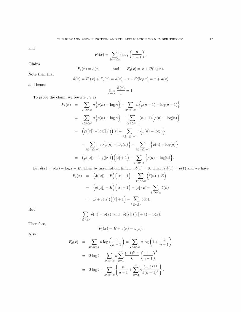
Theorem 13. limx→∞ (ρ(x) − log x) exists.

We shall present the beautiful proof of D. J. Newman [14]. His proof depends on the following conver-gence theorem, due to Ingham and dating back to 1929. The proof by Ingham uses Fourier analysis whileNewman’s proof of the convergence theorem uses only the theory of complex analysis. For comments uponand reviews of Newman’s proof of PNT, see the articles by D. Zagier [22] and J. Korevaar [11].

Theorem 14. (Convergence Theorem) Let {an} be a bounded sequence of complex numbers. For Re(s) =σ > 1, assume that

F (s) =∞∑

n=1

an

ns

is analytic in an open set containing the region Re(s) ≥ 1. Then the series∑∞

n=1an

ns converges for <(s) ≥ 1.

We shall return to the proof of the convergence theorem later. Let us assume its validity for now and useit to proof Theorem 13.

Proof of Theorem 13. Define

f(s) =∞∑

n=1

ρ(n)ns

=∞∑

n=1

∑

p≤n

log p

p

1

ns.

Clearly ρ(n) ≤ n and hence the series defining f(s) converges absolutely for σ > 2. We rewrite f as

f(s) =∑

p

logp

p

∞∑

n≥p

1ns

(35)

and use (18) with a = p to obtain

∞∑

n≥p

1ns

=1

(s − 1)ps−1+ s

∫ ∞

p

1 − {t}ts+1

dt, (36)


where {t} = t − [t] is the fractional part of the real number t. Define

Ap(s) =1ps

− 1ps − 1

+s(s − 1)

p

∫ ∞

p

1 − {t}ts+1

dt = − 1ps(ps − 1)

+s(s − 1)

p

∫ ∞

p

1 − {t}ts+1

dt,

so that∞∑

n≥p

1ns

=p

s − 1

(1

ps − 1+ Ap(s)

).

Using this in (35), we get

f(s) =1

s − 1

(∑

p

logp

ps − 1+∑

p

Ap(s) log p

). (37)

Clearly Ap(s) is analytic in Re(s) = σ > 0( one can appeal to the Dominated Convergence Theorem tojustify differentiating inside the integral to see this) and is bounded there by

1pσ(pσ − 1)

+|s(s − 1)|σpσ+1

.

For p ≥ 5 and σ > 1/2, we note that pσ − 1 > pσ/2 and hence

|Ap(s) log p| ≤ 2 logp

p2σ+

|s(s − 1)|σ

log p

pσ+1.

Clearly∑

p

log p

p2σ< ∞ and

∑

p

logp

pσ+1< ∞ for σ >

12.

By the Weierstrass M-test we conclude that the series defined by

A(s) =∑

p

Ap(s) logp

is analytic in Re(s) > 12 and by (37) we may express f(s) as

f(s) =1

s − 1

(∑

p

log p

ps − 1+ A(s)

). (38)

From the Euler Product Formula (11) for ζ(s), (yes! finally ζ(s) is coming to the scene), we haveζ(s) =

∏p (1 − p−s)−1. Upon logarithmic differentiation, we obtain

ζ′(s)ζ(s)

= −∑

p

log p

ps − 1, valid for σ > 1. (39)

Using (39) in (38) we see that

f(s) =1

s − 1

(−ζ′(s)

ζ(s)+ A(s)

). (40)

By Theorem 7, |ζ(1 + it)| 6= 0 and from Euler’s Product for ζ(s), we know that ζ(s) 6= 0 for σ > 1. Sinceζ(s) has a simple pole at s = 1, we see that (s − 1)ζ(s) 6= 0 in σ ≥ 1. We also observe that

−ζ′(s)ζ(s)

=1

s − 1+ g(s),


where g(s) is analytic at s = 1. Note then that

f(s) =1

s − 1

(1

s − 1+ g(s) + A(s)

).

Thus f(s) is meromorphic in an open set containing <(s) ≥ 1, holomorphic there except at s = 1, and withthe principal part

1(s − 1)2

+c

s − 1at s = 1, wheres c is a complex number.

We have proved that the function

F (s) = f(s) + ζ′(s) − cζ(s) =∞∑

n=1

an

ns,

where

an =∑

p≤n

logp

p− logn − c = ρ(n) − logn − c,

is analytic in an open set containing σ ≥ 1. By the Convergence Theorem we conclude that∑

n=1

an

n

converges. Our theorem now follows if we prove theClaim:

limn→∞

an = 0.

To prove the claim, let 0 < ε < 1 be given. By Cauchy criterion for convergence of a sequence, thereexists N0 > 0 such that for K ≥ N ≥ M > N0, we have

K∑

n=N

an

n≤ ε2 (41)

andN∑

n=M

an

n≥ −ε2. (42)

But then for N ≤ n ≤ K we have

an − aN =∑

N<p≤n

log p

p+ log N − logn ≥ log

(N

n

)≥ log

(N

K

).

We now choose K so that 1K

(K − N + 1) ≥ ε1+ε

and log(

NK

)> −ε. Then, for N ≤ n ≤ K, we have

an ≥ aN − ε. It follows thatK∑

n=N

an

n≥ (aN − ε)

K∑

n=N

1n

,

which is equivalently to

aN − ε ≤∑K

n=Nan

n∑Kn=N

1n

.


But∑K

n=N1n ≥ 1

K (K − N + 1) ≥ ε1+ε . Therefore,

aN − ε ≤

(K∑

n=N

an

n

)(1 + ε

ε

). (43)

Combining (41) and (43), we get

aN ≤ 2ε + ε2. (44)

On the other hand, for M ≤ n ≤ N , we have

aN − an =∑

n<p≤N

log p

p+ log

( n

N

)≥ log

( n

N

)≥ log

(M

N

).

We now choose M < N so that log(

MN

)≥ − ε

1−εand N−M+1

N≥ ε. This gives

an ≤ aN +ε

1 − ε

and henceN∑

n=M

an

n≤(

aN +ε

1 − ε

) N∑

n=M

1n

.

Assume aN + ε1−ε

≤ 0. Since∑N

n=M1n≥ 1

N(N − M + 1) ≥ ε, the above inequality implies that

N∑

n=M

an

n≤(

aN +ε

1 − ε

)ε.

From this and (42) we obtain

aN ≥ −ε(2 − ε)1 − ε

. (45)

If aN + ε1−ε

> 0, then

aN > − ε

1 − ε≥ −ε(2 − ε)

1 − ε,

since 0 < ε < 1. In either cases, (45) holds.

Combining (44) and (45), we conclude that

limn→∞

an = 0.

Note then that for any real number x, if we let n = [x], then

limx→∞

(ρ(x) − log x) = limn→∞

(ρ(n) − logn) = limn→∞

(an + c) = c

and the theorem follows.

The proof of PNT is now complete except for the proof of the Convergence Theorem. We shall presentthis proof now.

Proof of the Convergence Theorem: Suppose |an| ≤ K and let

F (s) =∞∑

n=1

an

ns


be analytic in an open set containing σ ≥ 1. Since we can replace an by an

K , we may assume K = 1. Fix w

with <(w) ≥ 1 and let ε > 0 be given. Let R = max{3ε , 1}. Then F (s + w) is analytic in <(s) ≥ 0. Hence

there exist positive numbers δ and M , depending on R, with 0 < δ < 12 such that F (s + w) is analytic and

|F (s + w)| ≤ M in − δ ≤ <(s), |s| ≤ R. (46)

Let Γ be the curve, with counter-clockwise orientation, given by

Γ = {s ∈ C| <(s) > −δ, |s| = R }⋃

{s ∈ C|<(s) = −δ, |s| ≤ R} .

Let Γr be the portion of Γ for which <(s) = σ > 0 and let Γl be the portion for which σ ≤ 0. By theCauchy residue theorem, we have

∫

Γ

F (s + w)N s

(1s

+s

R2

)ds = 2πiRes

(F (s + w)N s

(1s

+s

R2

); s = 0

)= 2πiF (w). (47)

On Γr, F (s + w) is given by its series and we may write it as F (s + w) = SN (s + w) + rN (s + w), where

SN (s + w) =N∑

n=1

an

ns+wand rN (s + w) =

∞∑

n=N+1

an

ns+w.

Note then that SN (s + w) is entire and hence∫

|s|=R

SN (s + w)N s

(1s

+s

R2

)ds = 2πiSN (w).

On the other hand,∫

|s|=R

SN (s + w)N s

(1s

+s

R2

)ds =

∫

Γr

SN (s + w)N s

(1s

+s

R2

)ds +

∫

−Γr

SN (s + w)N s

(1s

+s

R2

)ds,

where −Γr is the reflection of Γr through the origin. Therefore, we have

2πiSN (w) =∫

Γr

SN (s + w)N s

(1s

+s

R2

)ds +

∫

−Γr

SN (s + w)N s

(1s

+s

R2

)ds.

In the second integral we change variable from s to −s to obtain

2πiSN (w) =∫

Γr

SN (s + w)N s

(1s

+s

R2

)ds +

∫

Γr

SN (w − s)N−s

(1s

+s

R2

)ds. (48)

Combining (47) and (48), and noting that F (w + s) − SN (s + w) = rN (s), we get

2πi (F (w) − SN (w)) =∫

Γr

{rN (s + w)N s − SN (w − s)

N s

}(1s

+s

R2

)ds

+∫

Γl

F (s + w)N s

(1s

+s

R2

)ds. (49)

To estimate the integrals in (49), we observe the following bounds.

On |s| = R, we have∣∣∣∣1s

+s

R2

∣∣∣∣ =∣∣∣∣

s

|s|2+

s

R2

∣∣∣∣ =2|σ|R2

. (50)


On σ = −δ, |s| ≤ R, we have∣∣∣∣1s

+s

R2

∣∣∣∣ =∣∣∣∣R2 + s2

sR2

∣∣∣∣ ≤1δ

(R2 + |s|2

R2

)≤ 2

δ, (51)

where we have used the fact that |s| ≥ |σ| = δ.

Since |an| ≤ 1 and <(w) ≥ 1, we have, for s ∈ Γr,

|rN (s + w)| ≤∞∑

n=N+1

1nσ+1

≤∫ ∞

N

du

uσ+1du =

1σNσ

(52)

and

|SN (w − s)| ≤N∑

n=1

nσ−1 ≤ Nσ−1 +∫ N

0

uσ−1du = Nσ

(1N

+1σ

). (53)

Combining (50), (52) and (53) we obtain, for s ∈ Γr,∣∣∣∣[rN (s + w)N s − SN (w − s)

N s

](1s

+s

R2

)∣∣∣∣ ≤(

1σ

+1σ

+1N

)2σ

R2≤ 4

R2+

2RN

.

Noting that the length of Γr is πR and using the M − L theorem we have

∣∣∣∣∫

Γr

[rN (s + w)N s − SN (w − s)

N s

](1s

+s

R2

)ds

∣∣∣∣ ≤4π

R+

2π

N. (54)

On Γl, we write

∫

Γl

F (s + w)N s

(1s

+s

R2

)ds =

∫ R

−R

F (−δ + it + w)N−δ+it

(1

−δ + it+

−δ + it

R2

)idt

+∫

C1∪C2

F (s + w)N s

(1s

+s

R2

)ds, (55)

where

C1 = {s = σ + it ∈ Γ| − δ ≤ σ ≤ 0 and t > 0} and C2 = {s = σ + it ∈ Γ| − δ ≤ σ ≤ 0 and t < 0}.

By (46) and (50), with s = −σ + it, we have∣∣∣∣∫

C1∪C2

F (s + w)N s

(1s

+s

R2

)ds,

∣∣∣∣ ≤ 2∫ 0

−δ

MNσ 2|σ|R2

dσ

=−4M

R2

∫ 0

−δ

σNσdσ

=4M

R2

(1 − N−δ − δN−δ logN

log2 N

)≤ 4M

R2 log2 N. (56)

By (46) and (51), with s = −δ + it, we have∣∣∣∣∣

∫ R

−R

F (−δ + it + w)N−δ+it

(1

−δ + it+

−δ + it

R2

)idt

∣∣∣∣∣ ≤∫ R

−R

MN−δ 2δdt ≤ 4MR

δN δ. (57)

We now combine (56) and (57) to get


∣∣∣∣∫

Γl

F (s + w)N s

(1s

+s

R2

)ds

∣∣∣∣ ≤4MR

δN δ+

4M

R2 log2 N. (58)

Using (54) and (58) in (49) we get

|F (w) − SN (w)| ≤ 2R

+1N

+MR

δN δ+

M

R2 log2 N.

Since R ≥ 3ε , we can take N large enough to conclude that |F (w) − SN (w)| < ε thereby proving the fact that

the infinite series∑∞

n=1an

ns converges for <(s) ≥ 1. This completes the proof of the Convergence Theorem.

References

[1] Apostol, T. 1976. Introduction to Analytic Number Theory, New York. Springer-Verlag.

[2] Bak, J. and and Newman, D. 1991. Complex Analysis , New York. Springer-Verlag.[3] Bateman, P. and Diamond H. 1996. A Hundred Years of Prime Number Theorem. Amer. Math. Monthly 103 (1996), 729

- 741.[4] Chandrasekharan, K. 1970.Arithmetical Functions New York. Springer-Verlag.

[5] Goldberg, R. R. 1976. Methods of Real Analysis Second edition. New York: John Wiley and Sons.[6] Hardy G.H. and Wright, E.M., 1959. An Introduction to the Theory of Numbers. London: Oxford University Press.

[7] Hijab, Omar 2007. Introduction to Calculus and Classical Analysis, Second Edition New York. Springer-Verlag.[8] Ireland, K. and Rosen M. 1982. A Classical Introduction to Modern Number Theory New York: Springer-Verlag.

[9] Knopp, K. 1951. Theory and Application of Infinite Series Second edition. New York: Dover Publications, Inc.

[10] Knopp, M. 1993 Modular functions in analytic number theory Second edition. New York: Chelsea Publishing Co.[11] Korevaar, J. On Newman’s quick way to the prime number theorem Math. Intelligencer 4, 3. (1982), 108 - 110.

[12] Lebedev, N.N, (Translated by Silverman, R.R.) 1972. Special Functions and Their Applications New York: Dover Publi-cations, Inc.

[13] Marsden, J. E. and Hoffman, M. J. 1989. Basic Complex Analysis second edition. New York: W. H. Freeman and Company.[14] Newman, D. J. Simple analytic Proof of Prime Number Theorem Amer. Math. Monthly 87 (1980), 693 - 696.

[15] 1997. Analytic Number Theory New York: Springer Verlag.[16] Niven, I., Zuckerman, H., and Montgomery, H. 2000. Introduction to Number Theory, Fifth edition. New York: Wiley.

[17] Patterson, S. 1989. An Introduction to the Theory of the Riemann Zeta-Function Cambridge: Cambridge University Press.[18] Rademacher,H. 1977 Lectures on Elementary Number Theory Melbourne(FL), Krieger Publishing Co.

[19] Rosen K. 1993. Elementary Number Theory and Its Applications, Third edition. Reading MA: Addison-Wesley.[20] Titchmarsh, E. C. 1951. The Theory of the Riemann Zeta-function. London: Oxford University Press.

[21] 1939. Theory of Functions. London: Oxford University Press.[22] Zagier, D. Newman’s short proof the Prime Number Theorem Amer. Math. Monthly 104 (1997), 705 - 708.

Department of Mathematics, Rowan University, Glassboro, NJ 08028.

Department of Mathematics, Temple University, Philadelphia, PA 19122.

Date post:	11-May-2018
Category:	Documents
Upload:	hakhuong
View:	214 times
Download:	0 times

Introduction - Rowan Universityusers.rowan.edu/~hassen/Papers/distprime.pdf · Introduction This...

Documents