Introduction to Analytic Number Theory - tu-chemnitz.de · In number theory, the fundamental...

Introduction to

Analytic Number Theory

Selected Topics

Lecture Notes

Winter 2019/ 2020

Alois Pichler

Faculty of Mathematics

DRAFTVersion as of January 8, 2020

2

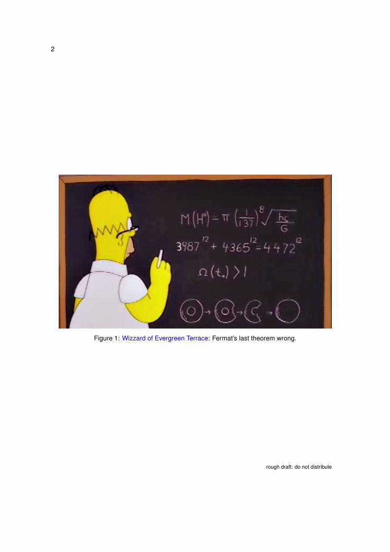
Figure 1: Wizzard of Evergreen Terrace: Fermat’s last theorem wrong.

rough draft: do not distribute

https://www.youtube.com/watch?v=Yj7XA3tiGUg

Contents

1 Introduction 7

2 Definitions 92.1 Elementary properties . . . . . . . . . . . . . . . . . . . . . . . . . . . . . . . . . 92.2 Fundamental theorem of arithmetic . . . . . . . . . . . . . . . . . . . . . . . . . . 122.3 Properties of primes . . . . . . . . . . . . . . . . . . . . . . . . . . . . . . . . . . 132.4 Chinese remainder theorem . . . . . . . . . . . . . . . . . . . . . . . . . . . . . . 142.5 Problems . . . . . . . . . . . . . . . . . . . . . . . . . . . . . . . . . . . . . . . . 16

3 Elementary number theory 193.1 Euler’s totient function . . . . . . . . . . . . . . . . . . . . . . . . . . . . . . . . . 193.2 Euler’s theorem . . . . . . . . . . . . . . . . . . . . . . . . . . . . . . . . . . . . . 213.3 Fermat Primality test . . . . . . . . . . . . . . . . . . . . . . . . . . . . . . . . . . 233.4 AKS Primality test . . . . . . . . . . . . . . . . . . . . . . . . . . . . . . . . . . . 233.5 Problems . . . . . . . . . . . . . . . . . . . . . . . . . . . . . . . . . . . . . . . . 24

4 Continued fractions 254.1 Generalized continued fraction . . . . . . . . . . . . . . . . . . . . . . . . . . . . 254.2 Regular continued fraction . . . . . . . . . . . . . . . . . . . . . . . . . . . . . . . 274.3 Elementary properties . . . . . . . . . . . . . . . . . . . . . . . . . . . . . . . . . 294.4 Problems . . . . . . . . . . . . . . . . . . . . . . . . . . . . . . . . . . . . . . . . 29

5 Bernoulli numbers and polynomials 315.1 Definitions . . . . . . . . . . . . . . . . . . . . . . . . . . . . . . . . . . . . . . . . 315.2 Summation and multiplication theorem . . . . . . . . . . . . . . . . . . . . . . . . 325.3 Fourier series . . . . . . . . . . . . . . . . . . . . . . . . . . . . . . . . . . . . . . 335.4 Umbral calculus . . . . . . . . . . . . . . . . . . . . . . . . . . . . . . . . . . . . 34

6 Gamma function 356.1 Equivalent definitions . . . . . . . . . . . . . . . . . . . . . . . . . . . . . . . . . . 356.2 Euler’s reflection formula . . . . . . . . . . . . . . . . . . . . . . . . . . . . . . . . 366.3 Duplication formula . . . . . . . . . . . . . . . . . . . . . . . . . . . . . . . . . . . 38

7 Euler–Maclaurin formula 397.1 Euler–Mascheroni constant . . . . . . . . . . . . . . . . . . . . . . . . . . . . . . 407.2 Stirling formula . . . . . . . . . . . . . . . . . . . . . . . . . . . . . . . . . . . . . 40

8 Summability methods 438.1 Silverman–Toeplitz theorem . . . . . . . . . . . . . . . . . . . . . . . . . . . . . . 438.2 Cesàro summation . . . . . . . . . . . . . . . . . . . . . . . . . . . . . . . . . . . 448.3 Euler’s series transformation . . . . . . . . . . . . . . . . . . . . . . . . . . . . . 448.4 Summation by parts . . . . . . . . . . . . . . . . . . . . . . . . . . . . . . . . . . 45

8.4.1 Abel summation . . . . . . . . . . . . . . . . . . . . . . . . . . . . . . . . 46

3

4 CONTENTS

8.4.2 Lambert summation . . . . . . . . . . . . . . . . . . . . . . . . . . . . . . 468.5 Abel’s summation formula . . . . . . . . . . . . . . . . . . . . . . . . . . . . . . . 478.6 Poisson summation formula . . . . . . . . . . . . . . . . . . . . . . . . . . . . . . 478.7 Borel summation . . . . . . . . . . . . . . . . . . . . . . . . . . . . . . . . . . . . 488.8 Abel–Plana formula . . . . . . . . . . . . . . . . . . . . . . . . . . . . . . . . . . 498.9 Mertens’ theorem . . . . . . . . . . . . . . . . . . . . . . . . . . . . . . . . . . . . 49

9 Euler’s product formula 519.1 Arithmetic functions . . . . . . . . . . . . . . . . . . . . . . . . . . . . . . . . . . 519.2 Examples of arithmetic functions . . . . . . . . . . . . . . . . . . . . . . . . . . . 519.3 Euler’s product formula . . . . . . . . . . . . . . . . . . . . . . . . . . . . . . . . 529.4 Problems . . . . . . . . . . . . . . . . . . . . . . . . . . . . . . . . . . . . . . . . 57

10 Multiplicative functions and Möbius inversion 5910.1 Dirichlet product and Möbius inversion . . . . . . . . . . . . . . . . . . . . . . . . 5910.2 The sum function . . . . . . . . . . . . . . . . . . . . . . . . . . . . . . . . . . . . 6110.3 Other sum functions . . . . . . . . . . . . . . . . . . . . . . . . . . . . . . . . . . 6110.4 Problems . . . . . . . . . . . . . . . . . . . . . . . . . . . . . . . . . . . . . . . . 62

11 Dirichlet Series 6511.1 Properties . . . . . . . . . . . . . . . . . . . . . . . . . . . . . . . . . . . . . . . . 6511.2 Abscissa of convergence . . . . . . . . . . . . . . . . . . . . . . . . . . . . . . . 6511.3 Problems . . . . . . . . . . . . . . . . . . . . . . . . . . . . . . . . . . . . . . . . 66

12 Mellin transform 6712.1 Inversion . . . . . . . . . . . . . . . . . . . . . . . . . . . . . . . . . . . . . . . . 6712.2 Perron’s formula . . . . . . . . . . . . . . . . . . . . . . . . . . . . . . . . . . . . 6912.3 Ramanujan’s master theorem . . . . . . . . . . . . . . . . . . . . . . . . . . . . . 7112.4 Convolutions . . . . . . . . . . . . . . . . . . . . . . . . . . . . . . . . . . . . . . 72

13 Riemann zeta function 7513.1 Related Dirichlet series . . . . . . . . . . . . . . . . . . . . . . . . . . . . . . . . 7513.2 Representations as integral . . . . . . . . . . . . . . . . . . . . . . . . . . . . . . 7713.3 Globally convergent series . . . . . . . . . . . . . . . . . . . . . . . . . . . . . . . 7913.4 Power series expansions . . . . . . . . . . . . . . . . . . . . . . . . . . . . . . . 8113.5 Euler’s theorem . . . . . . . . . . . . . . . . . . . . . . . . . . . . . . . . . . . . . 8213.6 The functional equation . . . . . . . . . . . . . . . . . . . . . . . . . . . . . . . . 8313.7 Riemann Hypothesis (RH) . . . . . . . . . . . . . . . . . . . . . . . . . . . . . . . 8713.8 Hadamard product . . . . . . . . . . . . . . . . . . . . . . . . . . . . . . . . . . . 87

14 Further results and auxiliary relations 8914.1 Occurrence of coprimes . . . . . . . . . . . . . . . . . . . . . . . . . . . . . . . . 8914.2 Exponential integral . . . . . . . . . . . . . . . . . . . . . . . . . . . . . . . . . . 8914.3 Logarithmic integral function . . . . . . . . . . . . . . . . . . . . . . . . . . . . . . 9014.4 Analytic extensions . . . . . . . . . . . . . . . . . . . . . . . . . . . . . . . . . . . 91

15 Prime counting functions 9315.1 Riemann prime counting functions and their relation . . . . . . . . . . . . . . . . 9315.2 Chebyshev prime counting functions and their relation . . . . . . . . . . . . . . . 9515.3 Relation of prime counting functions . . . . . . . . . . . . . . . . . . . . . . . . . 98


CONTENTS 5

16 The prime number theorem 10116.1 Zeta function on <(·) = 1 . . . . . . . . . . . . . . . . . . . . . . . . . . . . . . . 10116.2 The prime number theorem . . . . . . . . . . . . . . . . . . . . . . . . . . . . . . 10316.3 Consequences of the prime number theorem . . . . . . . . . . . . . . . . . . . . 104

17 Riemann’s approach by employing the zeta function 10717.1 Mertens’ function . . . . . . . . . . . . . . . . . . . . . . . . . . . . . . . . . . . . 10717.2 Chebyshev summatory function ψ . . . . . . . . . . . . . . . . . . . . . . . . . . 10717.3 Riemann prime counting function . . . . . . . . . . . . . . . . . . . . . . . . . . . 10817.4 Prime counting function π . . . . . . . . . . . . . . . . . . . . . . . . . . . . . . . 108

18 Further results 11118.1 Results . . . . . . . . . . . . . . . . . . . . . . . . . . . . . . . . . . . . . . . . . 11118.2 Open problems . . . . . . . . . . . . . . . . . . . . . . . . . . . . . . . . . . . . . 112

Bibliography 112

Version: January 8, 2020

6 CONTENTS


1Introduction

Even before I had begun my more detailedinvestigations into higher arithmetic, one ofmy first projects was to turn my attention tothe decreasing frequency of primes, towhich end I counted primes in severalchiliads. I soon recognized that behind allof its fluctuations, this frequency is onaverage inversely proportional to thelogarithm.

Gauß, letter to Encke, Dec. 1849

For an introduction, see Zagier [21]. Hardy and Wright [10] and Davenport [5], as well asApostol [2] are benchmarks for analytic number theory. Everything about the Riemann ζ functioncan be found in Titchmarsh [18, 19] and Edwards [7]. Other useful references include Ivaniecand Kowalski [12] and Borwein et al. [4].

Some parts here follow the nice and recommended lecture notes Forster [8] or Sander [17].This lecture note covers a complete proof of the prime number theorem (Section 16), which

is based on a new, nice and short proof by Newman, cf. Newman [14], Zagier [22].

Please report mistakes, errors, violations of copyrights, improvements or necessary comple-tions. Updated version of these lecture notes:https://www.tu-chemnitz.de/mathematik/fima/public/NumberTheory.pdf

Conjecture (Frank Morgan’s math chat). Suppose that there is a nice probability function P(x)that a large integer x is prime. As x increases by ∆x = 1, the new potential divisor x is primewith probability P(x) and divides future numbers with probability 1/x. Hence P gets multipliedby (1 − P/x), so that ∆P = (1 − P/x)P − P = −P2/x, or roughly

P′ = −P2/x.

The general solution to this differential equation is

P(x) =1

c + log x∼

1log x

.

7

https://www.tu-chemnitz.de/mathematik/fima/public/NumberTheory.pdf

8 INTRODUCTION

Figure 1.1: Gauss’ 1849 conjecture in his letter to the astronomer Johann Franz Encke,https://gauss.adw-goe.de/handle/gauss/199. Notably, all numbers π(·) are wrong in this letter:π(500 000) = 41 538, e.g.


https://gauss.adw-goe.de/handle/gauss/199

2Definitions

Before creation, God did just puremathematics. Then he thought it would bea pleasant change to do some applied.

John Edensor Littlewood, 1885–1977

N = 1, 2, 3, . . . the natural numbers

P = 2, 3, 5, . . . the prime numbers

Z = . . . ,−2,−1, 0, 1, 2, 3 . . . the integers

lcm: least common multiple, lcm(6, 15) = 30; sometimes also [m, n] = lcm(m, n)

gcd: greatest common divisor, gcd(6, 15) = 3. We shall also write (6, 15) = 3.

m ⊥ n: the numbers m and n are co-prime, i.e., (m, n) = 1

f ∼ g: the functions f and g satisfy limxf (x)g(x) = 1.

2.1 ELEMENTARY PROPERTIES

In number theory, the fundamental theorem of arithmetic, also called the unique factorizationtheorem or the unique-prime-factorization theorem, states that every integer greater than 1 ei-ther is prime itself or is the product of prime numbers, and that this product is unique, up to theorder of the factors.

Theorem 2.1 (Euclidean division1). Given two integers a, b ∈ Z with b , 0, there exist uniqueintegers q and r such that

a = b q + r and 0 ≤ r < |b|.

Proof. Assume that b > 0. Let r > 0 be such that a = b q + r (for example q = 0, r = a). If r < b,then we are done.

Otherwise, q2 := q1+1 and r2 := r1−b (with q1 := q, r1 := r) satisfy a = b q2+r2 and 0 ≤ r2 < r1.Repeating this process one gets eventually q = qk and r = rk such that a = b q + r and 0 ≤ r < b.

If b < 0, then set b′ := −b > 0 and a = b′q′ + r with some 0 ≤ r < b′ = |b|. With q := −q′ itholds that a = b′q′ + r = bq + r and hence the result.

Uniqueness: suppose that a = b q + r = b q′ + r ′ with 0 ≤ r, r ′ < |b|. Adding 0 ≤ r < |b| and−|b| < −r ′ ≤ 0 gives −|b| < r − r ′ ≤ |b|, that is |r − r ′ | ≤ |b|. Subtracting the two equations yieldsb(q′ − q) = r − r ′. If |r − r ′ | , 0, then |b| < |r − r ′ |, a contradiction. Hence r = r ′ and b(q′ − q) = 0.As b , 0 it follows that q′ = q, proving uniqueness.

1Euclid, 300 bc

9

10 DEFINITIONS

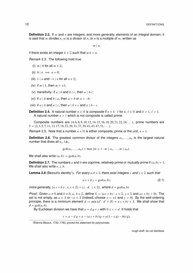
Definition 2.2. If m and n are integers, and more generally, elements of an integral domain, itis said that m divides n, m is a divisor of n, or n is a multiple of m, written as

m | n,

if there exists an integer k ∈ Z such that m k = n.

Remark 2.3. The following hold true.

(i) m | 0 for all m ∈ Z;

(ii) 0 | n =⇒ n = 0;

(iii) 1 | n and −1 | n for all n ∈ Z;

(iv) if m | 1, then m = ±1;

(v) transitivity: if a | b and b | c, then a | b c;

(vi) if a | b and b | a, then a = b or a = −b;

(vii) if a | b and a | c, then a | b + c and a | b − c.

Definition 2.4. A natural number n ∈ N is composite if n = k · ` for k, ` ∈ N and k > 1, ` > 1.A natural number n > 1 which is not composite is called prime.

Composite numbers are 4, 6, 8, 9, 10, 12, 14, 15, 16, 18, 20, 21, 22, 24, . . . , prime numbers areP = 2, 3, 5, 7, 11, 13, 17, 19, 23, 29, 31, 37, 39, 41, 43, 47, 51, . . . .Remark 2.5. Note that a number n ∈ N is either composite, prime or the unit, n = 1.

Definition 2.6. The greatest common divisor of the integers a1, . . . , an is the largest naturalnumber that dives all ai, i.e.,

gcd(a1, . . . , an) = max m ≥ 1: m | a1, . . . ,m | an .

We shall also write (a, b) := gcd(a, b).

Definition 2.7. The numbers a and b are coprime, relatively prime or mutually prime if (a, b) = 1.We shall also write a ⊥ b.

Lemma 2.8 (Bézout’s identity2). For every a, b ∈ Z there exist integers x and y ∈ Z such that

a x + b y = gcd(a, b); (2.1)

more generally, a x + b y : x, y ∈ Z = z · d : z ∈ Z, where d = gcd(a, b).

Proof. Given a , 0 and b , 0, a, b ∈ Z, define S := ax + by : x ∈ Z, y ∈ Z and ax + by > 0. Theset is not empty, as a ∈ S or −a ∈ S (indeed, choose x = ±1 and y = 0). By the well-orderingprinciple, there is a minimum element d := min d ′ : d ′ ∈ S = a s + b t ∈ S. We shall show thatd = gcd(a, b).

By Euclidean division we have that a = d q + r with 0 ≤ r < d. It holds that

r = a − d q = a − (a s + b t)q = a(1 − s q) − b(t q),

2Étienne Bézout, 1730–1783, proved the statement for polynomials.


2.1 ELEMENTARY PROPERTIES 11

and thus r ∈ S ∪ 0. As r < d = minS, it follows that r = 0, i.e., d | a; similarly, d | b and thusd ≤ gcd(a, b).

Now let c be any divisor of a and b, that is, a = c u and b = c v. Hence

d = a s + b t = cus + cvt = c(us + vt),

that is c | d and therefore c ≤ d, i.e., d ≥ gcd(a, b). Hence the result.

Corollary 2.9. There are integers x1, . . . , xn so that

gcd(a1, . . . , an) = x1 a1 + · · · + xn an.

Corollary 2.10. It holds that a and b are coprime,

(a, b) = 1 ⇐⇒ a s + b t = 1 (2.2)

for some s, t ∈ Z.

Proof. It remains to verify “ ⇐= ”: suppose that a s + b t = 1 and d is a divisor of a and b, i.e.,a = u d and b = v d. Then 1 = uds + vdt = d(us + vt), that is, d | 1, thus d = 1 and consequently(a, b) = 1.

Lemma 2.11 (Euclid’s lemma). If p ∈ P is prime and a · p a product of integers, then

p | (a · b) =⇒ p | a or p | b.

Theorem 2.12 (Generalization of Euclid’s lemma). If

n | (a · b) and (n, a) = 1, then n | b.

Proof. We have from (2.2) that r n + s a = 1 for some r, s ∈ Z. It follows that r n b + s a b = b.The first term is divisible by n. By assumption, n divides the second term as well, and hencen | b.

The extended Euclidean algorithm (Algorithm 1) computes the gcd of two numbers and thecoefficients in Bezout’s identity (2.1).

input : two integers a and boutput :gcd(a, b) and the coefficients of Bézout’s identity (2.1)

set (d, s, t, d ′, s′, t ′) = (a, 1, 0, b, 0, 1); initializewhile d ′ , 0 do

set q := d div d ′ integer divisionset (d, s, t, d ′, s′, t ′) = (d ′, s′, t ′, d − q · d ′, s − q · s′, t − q · t ′)

endreturn (d, s, t) it holds that d = gcd(a, b) = a s + b t

Algorithm 1: Extended Euclidean algorithm

Table 2.1 displays the results of the Euclidean algorithm for a = 2490 and b = 558: it holdsthat 13 ∗ 2490 − 58 ∗ 558 = 6 = gcd(a, b).


12 DEFINITIONS

q d s t d ′ s′ t ′

2490 1 0 558 0 1 initialize4 558 0 1 258 1 −4 2490/558 = 4 + 258/5582 258 1 −4 42 −2 9 558/258 = 2 + 42/2586 42 −2 9 6 13 −58 258/42 = 6 + 6/427 6 13 −58 0 −93 415 42/6 = 7 + 0

Table 2.1: Results of Algorithm 1 for a = 2490 and b = 558

2.2 FUNDAMENTAL THEOREM OF ARITHMETIC

The fundamental theorem of arithmetic, also called the unique factorization theorem or theunique-prime-factorization theorem, states that every integer greater than 1 either is a primenumber itself or can be represented as the product of prime numbers and that, moreover, thisrepresentation is unique, up to the order of factors.

Theorem 2.13 (Canonical representation of integers). Every integer n > 1 has the uniquerepresentation

n = pα11 · . . . · p

αωω , (2.3)

where p1 < p2 < · · · < pω and αi = 1, 2, . . . (αi > 0).

Proof. We need to show that every integer is prime or a product of primes. For the base case,n = 2 is prime. Assume the assertion is true for all numbers < n. If n is prime, there is nothingmore to prove. Otherwise, n is composite and there are integers so that n = ab and 1 < a ≤ b < n.By induction hypothesis, a = p1 · · · pj and b = q1 · · · qk , but then n = p1 · · · pj ·q1 · · · qk is a productof primes.

Uniqueness: suppose that n is a product of primes which is not unique, i.e.,

n = p1 · · · pj

= q1 · · · qk .

Apparently, p1 | n. By Euclid’s lemma (Lemma 2.11) we have that p1 divides one of the qis, q1,say. But q1 is prime, thus q1 = p1. Now repeat the reasoning to

n/p1 = p2 · · · pj and= q2 · · · qk,

so that q2 = p2, etc.

Theorem 2.14 (Euclid’s theorem). There exist infinity many primes.

Proof. Assume to the contrary that there are only finitely many primes, n, say, primes, whichare p1 = 2, p2 = 3, . . . , pn. Consider the natural number

q := p1 · p2 · . . . · pn.

If q + 1 is prime, then the initial list of primes was not complete.If q + 1 is not prime, then p | (q + 1) for some prime number p. But p | q, and hence, by

Remark 2.3 (iv), it follows that p | 1. But no prime number p satisfies p | 1 and hence q + 1 isprime, but not in the list.


2.3 PROPERTIES OF PRIMES 13

Theorem 2.15. Let p1 := 2, p2 := 3, etc. be the primes in increasing order. It holds that pn < 62n−3

for n ≥ 3.

Proof. The assertion is true for n = 3. It follows from the proof of Theorem 2.14 that pn+1 <

p1 · · · pn, thus pn+1 < 2 · 3 · 620· 621· · · 62n−3

= 62n−2, the result.

2.3 PROPERTIES OF PRIMES

Definition 2.16 (Prime gap). The n-th prime gap is gn := pn+1 − pn. (I.e., pn = 2 +∑n−1

i=1 gi.)

There exist prime gaps of arbitrary length.

Theorem 2.17 (Prime gap). For every g ∈ N there exist n ∈ N so that all n + 1, . . . , n + g are notprime, i.e., there is an m ∈ N so that pm+1 ≥ pm + g.

Proof. Define n := (g + 1)!, then d | (n + d) for every d ∈ 2, . . . , g + 1.

Remark 2.18. Alternatively, one may choose n := lcm (1, 2, 3, . . . , g + 1) in the preceding proof.

Definition 2.19 (Prime gaps). Let p ∈ P;

(i) if p + 2 ∈ P, then they are called twin primes;

(ii) if p + 4 ∈ P, they are called cousin primes;

(iii) if p + 6 ∈ P, then they are called sexy primes.3

Note that every prime p ∈ P is either p = 2, or p = 4k + 1 or p = 4k + 3.

Theorem 2.20. There are infinity many primes of the form 4k + 3.

Proof. Observe that

(4k + 1) · (4` + 1) = 4 (4k` + k + `) + 1 and (2.4)(4k + 3) · (4` + 3) = 4(4k` + 3k + 3` + 2) + 1. (2.5)

By reductio ad absurdum, suppose that there are only finitely many primes in

P3 :=p ∈ P : p = 4k + 3 for some k ∈ N

= 3, 7, 11, 19, . . . = p1, . . . , ps .

Consider N := p21 · · · p

2s + 2. By (2.5) and (2.4), N = 4k + 3 and thus 2 - N . Let q1, . . . , qr = N be

the prime factors of N . As 2 - N , we have that qi = 4ki + 1 or qi = 4ki + 3. If all factors were ofthe form qi = 4ki + 1, then N = 4k + 1 by (2.4), but N = 4k + 3. Hence there is some qi ∈ P3 forsome i. But qi | N and qi | p2

1 · · · p2s (these are all primes in P3), thus qi |

(N − p2

1 · · · p2s

), i.e., qi | 2

and this is a contradiction.

The following theorem represents the beginning of rigorous analytic number theory.

Theorem 2.21 (Dirichlet’s theorem on arithmetic progressions, 1837). For any two positive co-prime integers a, b there are infinity many primes of the form a + n b, n ∈ N.

Proposition 2.22. The following hold true:

3because 6 = sex in Latin


14 DEFINITIONS

(i) if 2n − 1 ∈ P, then n ∈ P;

(ii) if 2n + 1 ∈ P, then n = 2k for some k ∈ N.

Proof. Suppose that n < P, thus n = j ·` with 1 < j, ` < n. Recall that x`−y` = (x−y)·∑`−1

i=0 xi y`−i−1,thus

2n − 1 =(2j

)`− 1` =

(2j − 1

)·

`−1∑i=0

2j ·i

and thus 2j − 1 | 2n − 1. But 2n − 1 ∈ P by assumption and so this contradicts the assertion (ii),as 1 < j < n.

As for (ii) suppose that n , 2k , then n = j · `, with ` being odd and ` > 0. As above,

2n + 1 =(2j

)`− (−1)` =

(2j − (−1)

)·

`−1∑i=0

(−1)`−i−1 2j ·i

and hence 2j+1 | 2n+1. The result follows by reductio ad absurdum, as 2n+1 ∈ P by assumptionand 2 ≤ j < n.

Definition 2.23 (Fermat4 prime). The Fermat numbers are Fn := 22n + 1. Fn is a Fermat prime,if Fn is prime.

As of 2019, the only known Fermat primes are F0 = 3, F1 = 5, F2 = 17, F3 = 257 andF4 = 65 537. The factors of F6, . . . , F11 are known.

Theorem 2.24 (Gauss–Wantzel5 theorem). An n-sided regular polygon can be constructed withcompass and straightedge if and only if n is the product of a power of 2 and distinct Fermatprimes: in other words, if and only if n is of the form n = 2k p1 p2 . . . p2, where k is a nonnegativeinteger and the pi are distinct Fermat primes.

Definition 2.25 (Mersenne6 prime). Mersenne primes are prime numbers of the form Mn :=2n − 1.

Some Mersenne primes include M2 = 3, M3 = 7, M5 = 31, M7 = 127, M13 = 8191. As of 2018,51 Mersenne primes are known.

Proposition 2.26. It holds that

lcm(a, b) ∗ gcd(a, b) = a ∗ b.

2.4 CHINESE REMAINDER THEOREM

Definition 2.27. For m , 0 we shall say

a = b mod m

if m | (a − b).

4Pierre de Fermat, 1607–16655Pierre Wantzel, 1814–1848, French mathematician6Marin Mersenne, 1588–1648, a French Minim friar


2.4 CHINESE REMAINDER THEOREM 15

Remark 2.28. By Definition 2.2 we have that

a = b mod m iff a = b + k · m

for some k ∈ Z.


(i) Reflexivity: a = a mod m for all a ∈ Z;

(ii) Symmetry: a = b mod m, then b = a mod m for all a, b ∈ Z;

(iii) Transitivity: a = b mod m and b = c mod m, then a = c mod m;

In what follows we assume that a = a′ mod m and b = b′ mod m.

(iv) a ± b = a′ ± b′ mod m;

(v) a b = a′ b′ mod m;

(vi) c a = c a′ mod m for all c ∈ Z;

(vii) (compatibility with exponentiation) ak = a′k mod m for all k ∈ N;

(viii) p(a) = p(a′) mod m for all polynomials p(·) with integer coefficients;

Proposition 2.30. If gcd(a,m) | c, then the problem a x = c mod m has a solution (this is apossible converse to (vi)).

Proof. From (2.1) we have that d := gcd(a,m) = as+mt and hence c = a scd +mt cd . By assumption

we have that x = scd is an integer and it follows that c = ax + m · t cd , that is, ax = c mod m.

Remark 2.31. Suppose that 0 < a < p for a prime p. Then 1 = gcd(a, p) | 1 and hence theproblem ax = 1 has a solution, irrespective of a. Algorithm 1 provides numbers with 1 = a s + p t,that is a−1 = s mod p.

Theorem 2.32 (Chinese remainder theorem). Suppose that n1, . . . , nk are all pairwise coprimeand 0 ≤ ai < ni for every i. Then there is exactly one integer with x ≥ 0 and x < n1 · . . . · nk =: Nwith

x = a1 mod n1, (2.6)...

x = ak mod nk . (2.7)

Proof. The numbers ni and Ni := N/ni are coprime. Bézout’s identity provides integers Mi andmi such that Mi Ni + mi ni = 1. Set x :=

∑nj=1 a j Mj Nj . Recall that ni | Nj whenever i , j. Hence

x = ai Mi Ni = ai (1 − mi ni) = ai − ai mi ni mod ni and thus x solves (2.6)–(2.7).Suppose there were two solutions x and y of (2.6)–(2.7). Then ni | x − y and, as the ni are

all coprime, it follows that N | x − y. Hence x = y, as it is required that 0 ≤ x, y < N .

Theorem 2.33 (Lucas’s theorem7). For integers n, k and p prime it holds that(nk

)≡

∏i=0

(niki

)mod p,

where n = n` p` + n`−1 p`−1 + · · ·+ n0 and k = k` p` + k`−1 p`−1 + · · ·+ k0 are the base p expansionswith 0 ≤ ni, k < p.

7Édouard Lucas, 1842–1891, French mathematician


16 DEFINITIONS

Proof. If p is prime and 1 < n < p an integer, then p divides the numerator of(pk

)=

p ·(p−1) · · ·(p−k+1)k ·(k−1) · · ·1 ,

but not the denominator. Hence(pk

)= 0 mod p. It follows that (1 + x)p ≡ 1 + xp mod p.

Even more, p |(pi

k

)for every 0 < k < pi. Indeed, for pj ≤ k < pj+1 it holds that

(pi

k

)=

pi · · ·(pi − p

)· · ·

(pi − p2

)· · ·

(pi − pj

)· · ·

(pi − k + 1

)1 · 2 · · · p1 · · · p2 · · · pj · · · k

.

The power of p in the denominator are 1+2+· · ·+ j, the power of p in the numerator is i+1+2+· · ·+ jand thus p |

(pi

k

). It follows that (1 + x)p

i≡ 1 + xpi mod p.

It follows that

m∑k=0

(mk

)xk = (1 + x)m =

∏i=0

((1 + x)p

i )mi

≡∏i=0

(1 + xpi )mi

=∏i=0

mi∑ki=0

(mi

ki

)xki p

i

=∏i=0

p−1∑ki=0

(mi

ki

)xki p

i

=

m∑k=0

xk∏i=0

(mi

ki

)mod p

where in the final product, ki is the ith digit in the base p representation of k. The statement ofthe theorem follows by comparing the coefficients in the polynomial above.


n is prime ⇐⇒

(nk

)≡ 0 mod n for all k = 1, 2, . . . , n − 1.

Proof. If n = p is prime, then(nk

)=

(1k

)= 0 by Lucas’ theorem, as n = 1 · p.

Suppose that n is composite and k | n is the smallest divisor. Then(n−1k−1

)/k is not an integer.

Hence(nk

)= n ·

(n−1k−1

)/k , 0 mod n and thus the equivalence.

2.5 PROBLEMS

Exercise 2.1. Verify the output −3 · 12 + 1 · 42 = 6 = gcd(12, 42) of Algorithm 1.

Exercise 2.2. Show that 2−1 = 4, 3−1 = 5, 3−1 = 5, 4−1 = 2, 5−1 = 3 and 6−1 = 6 mod 7.

Exercise 2.3. Show that the set 3k + 2: k ∈ Z contains infinity many primes.

Exercise 2.4. Show that 6k + 5: k ∈ Z contains infinity many primes.

Exercise 2.5. If ak − 1 is prime (k > 1), then a = 2.

Exercise 2.6. If ak + 1 is prime (a, b > 1), then a is even and k = 2n for some n ≥ 1.

Exercise 2.7. Show that Fn = (Fn−1 − 1)2 + 1 and

(i) Fn = Fn−1 + 22n−1F0 . . . Fn−2,

(ii) Fn = F2n−1 − 2(Fn−2 − 1)2,


2.5 PROBLEMS 17

(iii) Fn = F0 · · · Fn−1 + 2.

Exercise 2.8 (Goldbach’s theorem). No two Fermat numbers share a common integer factorgreater than 1. (Hint: use (iii) in the preceding exercise.)

Exercise 2.9. Solve this riddle, https://www.spiegel.de/karriere/das-rotierende-fuenfeck-raetsel-der-woche-a-1276765.html.


https://www.spiegel.de/karriere/das-rotierende-fuenfeck-raetsel-der-woche-a-1276765.html

https://www.spiegel.de/karriere/das-rotierende-fuenfeck-raetsel-der-woche-a-1276765.html

18 DEFINITIONS


3Elementary number theory

178212 + 184112 = 192212,398712 + 436512 = 447212.

Fermat wrong

3.1 EULER’S TOTIENT FUNCTION

Definition 3.1 (Euler’s totient function1). Euler’s totient function is

ϕ(n) :=∑

m∈1,...,n(m,n)=1

1 = m ∈ 1, . . . , n : (m, n) = 1. (3.1)

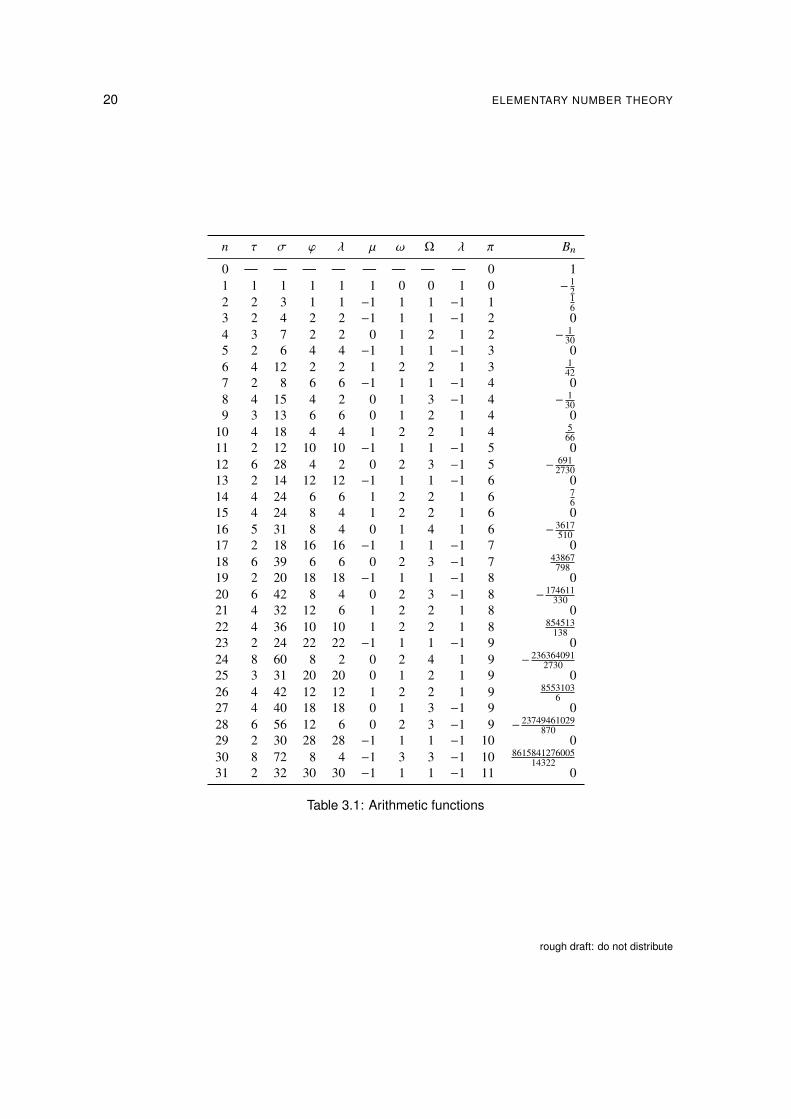
See Table 3.1 for some explicit values.

Theorem 3.2 (ϕ is multiplicative). It holds that

ϕ(m · n) = ϕ(m) · ϕ(n) if (m, n) = 1.

Proof. Let An := i ∈ N : i < n and (i, n) = 1. The Chinese remainder theorem (Theorem 2.32)provides a bijection An × Am → An ·m. Hence the result.

Theorem 3.3. For p prime it holds that

ϕ(pk ) = pk − pk−1 = pk(1 −

1p

).

Proof. The numbers m ≤ pk which satisfy gcd(pk,m

)> 1 are precisely m = p, 2 · p, . . . , pk−1 · p,

in total pk−1 numbers. Hence ϕ(pk ) = pk − pk−1, the result.

Theorem 3.4 (Euler’s product formula). It holds that

ϕ(n) = n ·∏p |n

(1 −

1p

);

in particularϕ(p) = p − 1. (3.2)

Proof. The fundamental theorem of arithmetic (Theorem 2.13) states that n = pα11 · . . . pαωω . Now

ϕ(n) =ω∏i=1

ϕ(pαi

i

)=

ω∏i=1

pαi

i

(1 −

1pi

)= n

ω∏i=1

(1 −

1pi

).

1Eulersche Phi-Funktion, eulersche Funktion

19

20 ELEMENTARY NUMBER THEORY

n τ σ ϕ λ µ ω Ω λ π Bn

0 — — — — — — — — 0 11 1 1 1 1 1 0 0 1 0 − 1

22 2 3 1 1 −1 1 1 −1 1 1

63 2 4 2 2 −1 1 1 −1 2 04 3 7 2 2 0 1 2 1 2 − 1

305 2 6 4 4 −1 1 1 −1 3 06 4 12 2 2 1 2 2 1 3 1

427 2 8 6 6 −1 1 1 −1 4 08 4 15 4 2 0 1 3 −1 4 − 1

309 3 13 6 6 0 1 2 1 4 0

10 4 18 4 4 1 2 2 1 4 566

11 2 12 10 10 −1 1 1 −1 5 012 6 28 4 2 0 2 3 −1 5 − 691

273013 2 14 12 12 −1 1 1 −1 6 014 4 24 6 6 1 2 2 1 6 7

615 4 24 8 4 1 2 2 1 6 016 5 31 8 4 0 1 4 1 6 − 3617

51017 2 18 16 16 −1 1 1 −1 7 018 6 39 6 6 0 2 3 −1 7 43867

79819 2 20 18 18 −1 1 1 −1 8 020 6 42 8 4 0 2 3 −1 8 − 174611

33021 4 32 12 6 1 2 2 1 8 022 4 36 10 10 1 2 2 1 8 854513

13823 2 24 22 22 −1 1 1 −1 9 024 8 60 8 2 0 2 4 1 9 − 236364091

273025 3 31 20 20 0 1 2 1 9 026 4 42 12 12 1 2 2 1 9 8553103

627 4 40 18 18 0 1 3 −1 9 028 6 56 12 6 0 2 3 −1 9 − 23749461029

87029 2 30 28 28 −1 1 1 −1 10 030 8 72 8 4 −1 3 3 −1 10 8615841276005

1432231 2 32 30 30 −1 1 1 −1 11 0

Table 3.1: Arithmetic functions


3.2 EULER’S THEOREM 21

Theorem 3.5 (Gauss). It holds that ∑d |n

ϕ(d) = n.

Proof. Consider the fractions 120,

110,

320,

15,

14,

310,

720,

25,

920,

12,

1120,

35,

1320,

710,

34,

45,

1720,

910,

1920,

11 . The frac-

tions with denominator n = 20 are precisely those with nominator coprime to 20, that is ϕ(20) = 8in total. There are ϕ(10) = 4 fractions with denominator 10, and ϕ(5) = 4 fractions with de-nominator 5, ϕ(4) = 2, ϕ(2) = 1 and ϕ(1) = 1. In total, there are n = 20 fractions, and thusn =

∑d |n ϕ(d).

3.2 EULER’S THEOREM

The multiplicative group of modulo n is (Z/nZ)× :=[a]n : gcd(a, n) = 1

.

Proposition 3.6. It holds that (Z/nZ)× = ϕ(n).

Proof. Suppose that n = pα11 · · · p

αωω . By the Chinese remainder theorem (Theorem 2.32) we

have thatZ/nZ Z/pα1

1 Z × · · · × Z/pαωω Z.

Similarly,(Z/nZ)×

(Z/pα1

1 Z)×× · · · ×

(Z/pαωω Z

)× .But

(Z/pαi

i Z)× = pαi

i − pαi−1i = ϕ(pαi

i ) and thus the result.

Theorem 3.7 (Lagrange’s theorem). Let (G, ·) be a finite group. The order (number of elements)of every subgroup H of G divides the order of G.

Proof. For a ∈ G define the (left) cosets aH := ah : h ∈ H . For the functions

fa,b : aH → bH

x 7→ ba−1x

it holds that f −1a,b= fb,a: the functions are invertible and bijective and thus the number of ele-

ments of aH and bH coincide for all a, b ∈ G. It follows that the order of G is the order of H × thenumber of distinct cosets.

Theorem 3.8 (Euler). It holds that

aϕ(n) = 1 mod n iff gcd(a, n) = 1. (3.3)

Proof. It holds thata, a2, . . . ak = 1 mod n

is a subgroup of (Z/nZ)×. By Lagrange’s theorem

we have that k | ϕ(n), i.e., k M = ϕ(n). It follows that

aϕ(n) = akM =(ak

)M= 1M = 1 mod n

and thus the result.

Corollary 3.9. If p is prime and p - a, then

ap−1 = 1 mod p. (3.4)



Proof. Apply (3.3) with (3.2).

Corollary 3.10 (Fermat’s little theorem). If p is prime, then

ap = a mod p.

Proof. If p | a, then a = 0 mod p and the assertion is immediate; if p - a, then the assertionfollows from (3.4).

Corollary 3.11 (Attributed to Euler). If p is an odd prime, it holds that

ap−1

2 = ±1 mod p, (3.5)

provided that (a, p) = 1.

Proof. Indeed, it holds that(a

p−12 − 1

) (a

p−12 + 1

)= ap−1 − 1 = 0 mod p. Hence, p | a

p−12 − 1 or

p | ap−1

2 + 1 and thus the result.

Definition 3.12 (Legendre symbol). Let p be an odd prime and a an integer. The Legendresymbol is (

ap

):= a

p−12 mod p and

(ap

)∈ −1, 0,+1.

Definition 3.13 (Jacobi symbol). Let n be any integer and a an integer. The Jacobi symbol is(ap1

)α1

· . . . ·

(a

pω

)αω,

where n = pα11 · . . . · p

αωω as in (2.3).

Definition 3.14 (Multiplicative order). The multiplicative order of a ∈ Z modulo n is the smallestpositive integer k = ordn(a) with

ak = 1 mod n.

Example 3.15. It holds that ord7(3) = 4, as 41 = 4 mod 7, 42 = 2 mod 7, but 43 = 64 = 1 mod 7.

Definition 3.16 (Carmichael function). The function λ(n), the smallest positive integer so that

aλ(n) = 1 for all a with (a, n) = 1

(cf. (3.3) and Table 3.1), is called Carmichael function.2

Corollary 3.17 (Carmichael). For n = pα11 · · · p

αωω define

λ(n) := lcm((p1 − 1)pα1−1

1 , . . . , (pω − 1)pαω−1ω

)then aλ(n) = 1 mod n.

Proof. By Euler’s theorem, aϕ(pαii ) = 1 mod pαi

i . Note, that ϕ(pαi

i ) | λ(n) by definition. It followsthat aλ(n) = 1 mod pαi

i for all i and thus aλ(n) = 1 mod n.

2Robert Daniel Carmichael, 1879–1967, American mathematician


3.3 FERMAT PRIMALITY TEST 23

Proposition 3.18. For all n and a it holds that

ordn(a) | λ(n) and λ(n) | ϕ(n).

Theorem 3.19 (Wilson’s theorem3). It holds that

(n − 1)! = −1 mod n iff n is prime.

Proof. The statement is clear for n = 2, 3 and 4.Suppose that n is composite, n = a b with a < b, then a | (n − 1)! and b | (n − 1)! and thus

(n − 1)! = 0 mod n. If n = q2, then q | 1 · 2 · · · q · · · 2q · · · (n − 1) and thus (n − 1)! = 0 mod n.Suppose now that n =: p is prime. Note that (p − 1)−1 = p − 1 = −1 mod p (indeed, (p −

1)2 = p2 − 2p + 1 = 1 mod p). Further, the product 2 · · · (p − 2) has even factors and for eachr ∈ 2, . . . , p − 2 it holds that r−1 ∈ 2, . . . , p − 2. Thus Wilson’s theorem.

3.3 FERMAT PRIMALITY TEST

By (3.5) we have that ap−1 = 1 mod p if (a, p) = 1. Note as well that the equation an−1 = 1mod n trivially holds true for a = 1 and it is also trivial for a = n − 1 = −1 mod n and n odd.

Definition 3.20 (Fermat pseudoprime). Suppose that a ∈ 2, 3, . . . , p − 2. If an−1 = 1 mod nwhen n is composite, then a is known as Fermat liar. In this case n is called a Fermat pseudo-prime to base a.

Definition 3.21 (Carmichael number). A composite number n is a Carmichael number if an−1 = 1mod n for all integers a.

Example 3.22. The first Carmichael number was given by Carmichael in 1910. The first are561 = 3 ∗ 11 ∗ 17, 1105 = 5 ∗ 13 ∗ 17, 1729 = 7 ∗ 13 ∗ 19, 2465 = 5 ∗ 17 ∗ 29, 2821 = 7 ∗ 13 ∗ 31,6601 = 7 ∗ 23 ∗ 41, 8911 = 7 ∗ 19 ∗ 67.

Theorem 3.23. There are infinitely many Camichael numbers.

Theorem 3.24 (Korselt’s criterion,4 1899). A positive composite integer n is a Carmichael num-ber iff n is square–free and for all prime divisors p of n, it is true that p − 1 | n − 1.

3.4 AKS PRIMALITY TEST

A starting point for the AKS primality test5 (Algorithm 2) is the following theorem.

Theorem 3.25 (AKS). It holds that

n is prime ⇐⇒ (x + a)n ≡ xn + a mod n

for all (a, n) = 1.

Proof. Proposition 2.34 together with Fermat’s little theorem.

Remark 3.26 (Primes is P). The AKS algorithm was the first to determine whether any givennumber is prime or composite within polynomial time.

3John Wilson, 1741–1793, British mathematician4Alwin Reinhold Korselt, 1864 (Mittelherwigsdorf)–1947 (Plauen)5Also known as Agrawal–Kayal–Saxena primality test; published by Manindra Agrawal, Neeraj Kayal and Nitin Sax-

ena in 2002.



input :an integer noutput :n is prime or n is compositeif n = ak for some a ∈ N and k > 1 then

return n is compositeendfind smalles r such that ordr (n) > log(n)2.if 1 < (a, n) < n for some a < r then

return n is compositeendif a < n then

return n is primeendfor a = 1 to

√ϕ(r) log n do

if (x + a)n , xn + a mod (xr − 1, n) thenreturn n is composite

endendreturn n is prime

Algorithm 2: AKS primality test

3.5 PROBLEMS

Exercise 3.1. Show that the function ω is additive (in the sense of Definition 9.2 below), whileΩ is completely additive.

Exercise 3.2. Discuss additivity/ multiplicativity for the other arithmetic functions introduced inthis section.

Exercise 3.3. Show that∑n

k=1 τ(k) =∑n

k=1

⌊nk

⌋and

∑nk=1 σ(k) =

∑nk=1 k

⌊nk

⌋.


4Continued fractions

80 435 758 145 817 5153 −80 538 738 812 075 9743 +12 602 123 297 335 6313 = 42.

The Hitchhiker’s Guide to the Galaxy

For the standard theory see Wall [20] or Duverney [6]; for the relation to orthogonal polyno-mials see Khrushchev [13].

4.1 GENERALIZED CONTINUED FRACTION

Definition 4.1 (Continued fraction). Different notations for the (generalized) continued fraction

rn := b0 +a1

b1 +a2

b2 +. . .

. . .

bn +an

bn

(4.1)

include

rn = b0 +nKi=1

aibi= b0 +

a1 |

| b1+

a2 |

| b2+ · · · +

an |

| bn= b0 +

a1b1 +

a2b2 +

. . .an

bn.

Theorem 4.2. For every n ≥ 0 we have that rn =pn

qn, where

p−1 = 1,q−1 = 0,

p0 = b0,q0 = 1,

pn = bnpn−1 + anpn−2,qn = bnqn−1 + anqn−2.

(4.2)

Proof. Observe first that r0 = b0 =p0q0

and r1 = b0 +a1b1=

b1b0+a1b1

=p1q1

. For n = 2 we obtain

r2 = b0 +a1

b1+a2b2

=b2 (b1b0+a1)+a2b0

b2b1+a21 =p2q2

. We continue by induction. It holds that

rn = b0 +a1

b1 + . . .an−1

bn−1 +an

bn +an+1

bn+1

=:p′nq′n.

25

26 CONTINUED FRACTIONS

Replacing bn in (4.1) by bn +an+1

bn+1we obtain by the induction hypothesis that

p′n = *,bn +

an+1

bn+1+-

pn−1 + anpn−2 and

q′n = *,bn +

an+1

bn+1+-

qn−1 + anqn−2,

which implies

bn+1p′n = bn+1 (bnpn−1 + anpn−2) + an+1pn−1 andbn+1q′n = bn+1

(bnqn−1 + anqn−2

)+ an+1qn−1,

and, again by the induction hypothesis,

bn+1p′n = bn+1pn + an+1pn−1 andbn+1q′n = bn+1qn + an+1qn−1.

Now set pn+1 := bn+1p′n and qn+1 := bn+1q′n to get rn+1 =pn+1qn+1

.

Theorem 4.3 (Determinant formula). For every n ≥ 1 it holds that

pn−1 qn − pn qn−1 = (−1)na1a2 . . . an and (4.3)

rn − rn−1 = (−1)n−1 a1a2 . . . an

qn−1 qnif qnqn−1 , 0;

further it holds that

pn−2 qn − pn qn−2 = (−1)n−1a1a2 . . . an−1 · bn and

rn − rn−2 = (−1)na1a2 . . . an · bn

qn qn−2.

Proof. For n = 0, the statement reads 1 · 1 − b0 · 0 = 1, which is the assertion. By inductionand (4.2),

pn−1qn − pnqn−1 = pn−1(bnqn−1 + anqn−2) − (bnpn−1 + anpn−2)qn−1

= −an(pn−2qn−1 − pn−1qn−2

).

Further we have that

pn−2qn − pnqn−2 = pn−2(bnqn−1 + anqn−2

)− (bnpn−1 + anpn−2) qn−2

= bn(pn−2qn−1 − pn−1qn−2

)= (−1)n−1a1a2 . . . an−1 · bn

by (4.3).The remaining assertions follow by dividing accordantly.

Corollary 4.4. It holds that rn = b0 −∑n

k=1(−1)k a1a2...ak

qk−1 qk.


4.2 REGULAR CONTINUED FRACTION 27

4.2 REGULAR CONTINUED FRACTION

Remark 4.5 (Equivalence transformation). For any sequence ci with ci , 0 it holds that

rn = b0 +a1

b1 +a2

b2 +a3

b3 +a4

b4 + . . .

= b0 +c1a1

c1b1 +c1c2a2

c2b2 +c2c3a3

c3b3 +c3c4a4

c4b4 + . . .

.

If we choose c1 := 1a1

, c2 := a1a2

, c3 =a2

a1a3and generally cn+1 := 1

cnan+1we get that rn = b0+

nKi=1

ai

bi=

b0 +nKi=1

1cibi

.

Definition 4.6 (Regular continued fraction). The continued fraction with ai = 1 is called regular.The convergents of a regular continued fraction are denoted pn

qn=: [b0; b1, . . . , bn].

Remark 4.7. The first convergents are b0, b1b0+1b1

, b2 (b1b0+1)+b0b2b1+1 , b3

(b2 (b1b0+1

)+b0+(b1b0+1)

b3 (b2b1+1)+b1, etc.

Remark 4.8. Note, that [b0; b1, . . . , bn−1, bn, 1] = [b0; b1, . . . , bn−1, bn+1] and the continued fractionof a rational thus is not unique.

Note that the denominators of a regular continued fracttion satisfy pn−1qn − pnqn−1 = ±1by (4.3) and thus they are relatively prime, gcd(qn, qn−1) = 1, by Bézout’s identity (2.1) andCorollary 2.10. By the same equality it follows that pn and qn are coprime as well, so rn =

pn

qnis

free of common factors.

Lemma 4.9 (Reciprocals). It holds that [0; b1, . . . bn] = 1[b1; b2,...bn] .

Consider a real number r. Let i := brc be the integer part of r and f := r − i be the fractionalpart of r. Then the continued fraction representation of r is [i; a1, a2, . . .], where 1/ f = [a1; a2, . . .]is the continued fraction representation of 1/ f .

Example 4.10 (Euclid’s algorithm). Table 2.1 displays the extended Euclidean algorithm (Algo-rithm 1) for a = 2490 and b = 558. The successive fractions of −t′/s′ are

4,

4 +12= 4.5,

4 +1

2 + 16=

5813= 4.4615 . . . ,

4 +1

2 + 16+ 1

7

=41593=

2490558

= 4.4623 . . . ,

which are improved approximations of ab . The sequence of integer quotients is b0 = 4, b1 = 2,

b2 = 6 and b3 = 7, cf. Table 2.1.

Remark 4.11. Euclid’s algorithm (Algorithm 1) produces for a/b and for ma/mb the same se-quence q of integer quotients (m ∈ Z\0). For the reduced fraction a/b we have that s a + t b =



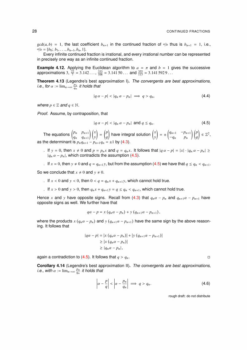
gcd(a, b) = 1, the last coefficient bn+1 in the continued fraction of a/b thus is bn+1 = 1, i.e.,a/b = [b0; b1, . . . , bn−1, bn, 1].

Every infinite continued fraction is irrational, and every irrational number can be representedin precisely one way as an infinite continued fraction.

Example 4.12. Applying the Euclidean algorithm to a = π and b = 1 gives the successiveapproximations 3, 22

7 = 3.142 . . . , 333106 = 3.141 50 . . . and 355

113 = 3.141 592 9 . . .

Theorem 4.13 (Legendre’s best approximation I). The convergents are best approximations,i.e., for α := limn→∞

pn

qnit holds that

|q α − p| < |qn α − pn | =⇒ q > qn, (4.4)

where p ∈ Z and q ∈ N.

Proof. Assume, by contraposition, that

|q α − p| < |qn α − pn | and q ≤ qn. (4.5)

The equations(pn pn+1qn qn+1

) (xy

)=

(pq

)have integral solution

(xy

)= ±

(qn+1 −pn+1−qn pn

) (pq

)∈ Z2,

as the determinant is pnqn+1 − pn+1qn = ±1 by (4.3).

. If y = 0, then x , 0 and p = pnx and q = qnx. It follows that |q α − p| = |x | · |qn α − pn | ≥|qn α − pn |, which contradicts the assumption (4.5).

. If x = 0, then y , 0 and q = qn+1y, but from the assumption (4.5) we have that q ≤ qn < qn+1.

So we conclude that x , 0 and y , 0.

. If x < 0 and y < 0, then 0 < q = qnx + qn+1y, which cannot hold true.

. If x > 0 and y > 0, then qnx + qn+1y = q ≤ qn < qn+1, which cannot hold true.

Hence x and y have opposite signs. Recall from (4.3) that qnα − pn and qn+1α − pn+1 haveopposite signs as well. We further have that

qα − p = x(qnα − pn

)+ y

(qn+1α − pn+1

),

where the products x(qnα − pn

)and y

(qn+1α − pn+1

)have the same sign by the above reason-

ing. It follows that

|qα − p| = x(qnα − pn

) + y(qn+1α − pn+1

) ≥ x

(qnα − pn

) ≥ |qnα − pn | ,

again a contradiction to (4.5). It follows that q > qn.

Corollary 4.14 (Legendre’s best approximation II). The convergents are best approximations,i.e., with α := limn→∞

pn

qnit holds that

α −

pq

<

α −

pnqn

=⇒ q > qn. (4.6)


4.3 ELEMENTARY PROPERTIES 29

Proof. Assume that q ≤ qn. Then we may multiply with (4.6) to obtain |q α − p| < |qn α − pn |,but the preceding theorem implies q > qn. This contradicts the assumption and hence theassertion.

Theorem 4.15. For α := limn→∞pn

qnit holds that

bn+2qn qn+2

<α −

pnqn

<

1qn qn+1

<1q2n

.

Further, for α irrational we have that p0q0<

p2q2< · · · < α < · · · <

p3q3<

p1q1

.

Proof. The assertion follows from (4.3), as the convergents rn =pn

qn, rn+1 and rn+2 oscillate

around α.

4.3 ELEMENTARY PROPERTIES

Theorem 4.16 (Gauss’s continued fraction). Let f0, f1, f2, . . . be a sequence of functions sothat f i−1(z) − f i (z) = ki z f i+1(z), then

f1(z)f0(z)

=1

1 +k1z

1 +k2z

1 +k3z

1 + . . .

.

4.4 PROBLEMS

Exercise 4.1 (Golden ratio). Show that φ = 1+√

52 = [1; 1, 1, 1, . . . ].

Exercise 4.2. Show that√

2 = [1; 2, 2, 2, . . . ].

Exercise 4.3. Show that√

5 = [2; 4, 4, 4, . . . ].




5Bernoulli numbers and polynomials

1729 = 13 + 123 = 93 + 103.

Taxicab

5.1 DEFINITIONS

Definition 5.1. Bernoulli numbers1 Bk , k = 0, 1, . . . , are defined by

zez − 1

=1

1 + z2! +

z2

3! + . . .

=∑k=0

Bk

k!zk (5.1)

= 1 −z2+

z2

12−

z4

720+

z6

30 240−

z8

1 209 600+

z10

47 900 160∓ . . . ;

Bernoulli polynomials arez ezx

ez − 1=

∞∑k=0

Bk (x)k!

zk . (5.2)

Table 3.1 presents some explicit Bernoulli numbers and Table 5.1 below lists the first Bernoullipolynomials.

Remark 5.2. It is evident by comparing (5.1) and (5.2) that

Bk = Bk (0). (5.3)

Remark 5.3. Note that coth z = cosh zsinh z =

ez+e−z

ez−e−z =e2z−1+2e2z−1 =

2e2z−1 + 1 is an odd function, thus

z2

cothz2=

zez − 1

+z2=

∞∑k=0

B2k(2k)!

z2k

and it follows thatB2k+1 = 0 (5.4)

for k ≥ 1 (note, however, that B1 = −12 ).

Proposition 5.4 (Explicit formula). Bernoulli polynomials (and thus Bernoulli numbers) aregiven explicitly by

Bk (x) =k∑

n=0

1n + 1

n∑`=0

(−1)`(n`

)(` + x)k . (5.5)

1Jacob I Bernoulli, 1654–1705

31

32 BERNOULLI NUMBERS AND POLYNOMIALS

Proof. It holds that z = log(1 − (1 − ez )

)= −

∑n=0

(1−ez )n+1

n+1 and thus

z ez x

ez − 1= ezx

∞∑n=0

(1 − ez

)nn + 1

=

∞∑n=0

1n + 1

n∑`=0

(−1)`(n`

)ez(x+`)

=

∞∑k=0

zk

k!·

∞∑n=0

1n + 1

n∑`=0

(−1)`(n`

)(` + x)k .

The sum over n in the latter display terminates at k, as x 7→ (` + x)k is a polynomial of degree kand thus

∑n`=0(−1)`

(n`

)(`+x)k = 0 for n ≥ k . The assertion follows by comparing coefficients.

Remark 5.5 (Translation). We have that

z ez(x+y)

ez − 1=

∞∑k=0

(z y)k

k!·

∞∑`=0

B` (x)`!

z` =∞∑k=0

zk

k!

k∑`=0

(k`

)B` (x)yk−`

so that

Bk (x + y) =k∑`=0

(k`

)B` (x) yk−`

by comparing with (5.2).

Remark 5.6 (Symmetry). Comparing the coefficients in the identity z e(1−x )z

ez−1 = −z e−xz

e−z−1 revealsthat

Bk (1 − x) = (−1)kBk (x). (5.6)

In particular we find that Bk (1) = (−1)kBk .

Remark 5.7. Differentiating (5.2) with respect to x and comparing the coefficients at zk revealsthat

B′k (x) = k · Bk−1(x). (5.7)

5.2 SUMMATION AND MULTIPLICATION THEOREM

Theorem 5.8 (Faulhaber’s formula2). For p = 0, 1, 2, . . . , x ∈ R and n ∈ N (actually n ∈ Z, if weset

∑bk=a := −

∑a−1k=b+1 whenever b < a) it holds that

n−1∑k=0

(k + x)p =Bp+1(n + x) − Bp+1(x)

p + 1. (5.8)

Proof. Set Sp (n) :=∑n−1

k=0 (k + x)p, then the generating function is

∞∑p=0

zpSp (n)

p!=

n−1∑k=0

∞∑p=0

(k + x)p

p!zp =

n−1∑k=0

e(k+x)z =e(n+x)z

ez − 1−

exz

ez − 1.

=∑k=0

zk−1 Bk (n + x) − Bk (x)k!

,

from which the assertion follows by comparing the coefficients (k = p + 1).

2Johann Faulhaber, 1580–1635


5.3 FOURIER SERIES 33

Proposition 5.9 (Multiplication theorem). For m ∈ N holds that

Bk (mx) = mk−1m−1∑`=0

Bk

(x +

`

m

).

Proof. Indeed, the result follows by comparing the coefficients in the identity

m−1∑`=0

∞∑k=0

Bk

(x +

`

m

)zk

k!=

m−1∑`=0

ze(x+ `

m

)z

ez − 1=

zexz

ez − 1e

zmm − 1

ez/m − 1= z

exz

ez/m − 1.

5.3 FOURIER SERIES

In what follows we define the periodic function (with period 1)

βk (x) := Bk (x − bxc), x ∈ R. (5.9)

It follows from (5.4) and (5.6) that βk is continuous for k ≥ 2. Even more, by (5.7), βk ∈ C (k−2) (R).

Theorem 5.10. The Bernoulli polynomials are given, for k ≥ 1, by the Fourier series3

Bk (x) = −k!

(2πi)k∑n∈Z,n,0

e2πinx

nk= −2 · k!

∞∑n=1

cos(2πnx − kπ

2

)(2πn)k

, x ∈ (0, 1). (5.10)

Proof. Consider the function x 7→ z ezx

ez−1 . Its Fourier coefficients, for n ∈ Z, are

ˆ 1

0e−2πinx z ezx

ez − 1dx =

zez − 1

ˆ 1

0ex(z−2πin) dx =

zez − 1

ex(z−2πin)

z − 2πin

1

x=0

=z

ez − 1ez − 1

z − 2πin=

zz − 2πin

.

The Fourier series thus is∑k=0

Bk (x)zk

k!=

z ezx

ez − 1=

∑n∈Z

e2πinx zz − 2πin

= 1 −∑n,0

e2πinx z2πin

11 − z

2πin

= 1 −∑n,0

e2πinx∞∑k=1

( z2πin

)k= 1 −

∞∑k=1

zk

k!· k!

∑n,0

e2πinx

(2πin)k.

The result follows by comparing the coefficients.

3Recall that sin(x + π

2)= cos x and cos

(x + π

2)= − sin x.


34 BERNOULLI NUMBERS AND POLYNOMIALS

Polynomial Bk (x) Fourier series βk (x)

B0(x) = 1B1(x) = x − 1

2 = −2 ·∑∞

n=1sin 2πnx

2πn sawtooth wave (5.11)B2(x) = x2 − x + 1

6 = 4 ·∑∞

n=1cos 2πnx(2πn)2

B3(x) = x3 − 32 x2 + 1

2 x = 12 ·∑∞

n=1sin 2πnx(2πn)3

B4(x) = x4 − 2x3 + x2 − 130 = −48 ·

∑∞n=1

cos 2πnx(2πn)4

B5(x) = x5 − 52 x4 + 5

3 x3 − x6 = −240 ·

∑∞n=1

sin 2πnx(2πn)5

Table 5.1: Bernoulli polynomials

5.4 UMBRAL CALCULUS

As a formal power series and interpreting Bk as Bk we have eBx = xex−1 and thus e(B+n)x = x enx

ex−1and also

e(B+n)x − eBx = xenx − 1ex − 1

= x(e0x + ex + · · · + e(n−1)x

),

and by comparing the coefficients of xk+1

k! thus (B+n)k+1−Bk+1

k+1 = 0k + 1k + · · · + (n − 1)k , i.e.,

0k + 2k + · · · + (n − 1)k =1

k + 1

(nk+1 +

(k + 1

1

)B1nk +

(k + 1

1

)B2nk−1 + · · · +

(k + 1

k

)Bkn

).


6Gamma function

6.1 EQUIVALENT DEFINITIONS

Definition 6.1. Euler’s integral of the second kind, aka. Gamma function, is (the analytic exten-sion) of

Γ(s) :=ˆ ∞

0xs−1e−x dx, <(s) > 0.

Remark 6.2. By integration by parts it holds that Γ(s + 1) = s Γ(s), so the analytic extension toC\0,−1,−2, . . . is apparent. The derivatives are

Γ(k) (s) =

ˆ ∞0

xs−1 (log x

)k e−x dx, <(s) > 0. (6.1)

Proposition 6.3 (Gauß’ definition of the Γ-function). It holds that

Γ(s) = limn→∞

n! ns

s(s + 1) · · · (s + n), s < 0,−1,−2, . . . . (6.2)

Proof. Recall that(1 − x

n

)n→ e−x as n → ∞ for every x ∈ C. Then

ˆ n

0

(1 −

xn

)nxs−1 dx =

ˆ ∞0

fn(x)xs−1 dx −−−−→n→∞

ˆ ∞0

e−x xs−1 dx

for fn(x) =(1 − x

n

)n· 1(0,n) by Lebesgue’s dominated convergence theorem. By integration by

parts we obtainˆ n

0+

(1 −

xn

)nxs−1 dx =

(1 −

xn

)n xs

s

n

x=0++

ˆ n

0+

(1 −

xn

)n−1 xs

sdx

=1s·

ˆ n

0+

(1 −

xn

)n−1xs dx.

Repeating the argument n − 1 times givesˆ n

0+

(1 −

xn

)nxs−1 dx =

n − 1n

1s(s + 1)

·

ˆ n

0+

(1 −

xn

)n−2xs+1 dx

=(n − 1)(n − 2) · · · 1

nn−11

s(s + 1) · · · (s + n − 1)

ˆ n

0xs+n−1 dx

=n!nn

ns+n

s(s + 1) · · · (s + n)=

n! ns

s(s + 1) · · · (s + n)


Corollary 6.4. It holds that

Γ(s) =1s

∏n=1

(1 + 1

n

)s1 + s

n

. (6.3)

35

36 GAMMA FUNCTION

Proof. Note that(1 + 1

1

) (1 + 1

2

). . .

(1 + 1

n−1

)= 2

1 ·32 · . . . ·

nn−1 = n, so the result follows from (6.2).

Theorem 6.5 (Schlömilch formula, Weierstrass’ definition). It holds that

Γ(s) =e−γs

s

∏n=1

es/n

1 + sn

, (6.4)

where γ is the Euler–Mascheroni constant.1

Proof. Use that∑n

j=11j − log n −−−−→

n→∞γ and thus exp

(−γs +

∑nj=1

sj

)∼ ns. The result follows

with (6.3).

Theorem 6.6. The Taylor series expansion is given by

log Γ(1 + s) = −γs +∑k=2

ζ (k)k

(−s)k, |s | < 1.

Proof. With (6.4) we get

log(s · Γ(s)

)= −γs +

∑n=1

( sn− log

(1 +

sn

))= −γs +

∑n=1

*,

sn+

∑k=1

(−1)k1k

( sn

)k+-

= −γs +∑k=2

(−1)k1k

∑n=1

( sn

)k= −γs +

∑k=2

(−s)kζ (k)

k, (6.5)

the result.

Corollary 6.7. It holds that Γ(s) = 1s −γ+

s2

(γ2 + π2

6

)+O

(s2

)and Γ(s+1) = 1−γs+ s

2

(γ2 + π2

6

)+

O(s2

). The residues at s = −n (n = 0, 1, . . . ) are given by

Γ(s) =(−1)n

(s + n) · n!+ O(1). (6.6)

6.2 EULER’S REFLECTION FORMULA


π coth πx =1x+

∞∑n=1

2xx2 + n2 , x 66∈ Z. (6.7)

Proof. Consider the function t 7→ cosh(x t) for x > 0 on (−π, π). The function is even, thus theTaylor series expansion is cosh xt = a0

2 +∑

n=1 an cos nt with

a0 =1π

ˆ π

−πcosh xt dt =

2x π

sinh xπ

1Lorenzo Mascheroni, 1750–1800


6.2 EULER’S REFLECTION FORMULA 37

and

an =1π

ˆ π

−πcos nt cosh xt dt =

1π

ˆ π

−π

eint + e−int

2ext + e−xt

2dt

=1

4π

(e(in+x)t

in + x+

e(in−x)t

in − x+

e(−in+x)t

−in + x+

e(−in−x)t

−in − x

)

π

t=−π

=(−1)n

4π

(exπ − e−xπ

in + x+

e−xπ − exπ

in − x+

exπ − e−xπ

−in + x+

e−xπ − exπ

−in − x

)=

(−1)n

2π4x

n2 + x2 sinh πx

and thus

cosh xt =sinh πxπx

+sinh πxπ

∑n=1

(−1)n2x cos ntn2 + x2 . (6.8)

The result follows for t = π.

Proposition 6.9 (Euler’s infinite product for the sine function). It holds that

sin πx = πx∞∏k=1

(1 −

x2

k2

). (6.9)

Proof. Set f (x) := sin πx thus f ′(x)f (x) = π cot πx; set g(x) := πx

∏∞k=1

(1 − x2

k2

)and it follows that

g′(x)g(x)

=1x−

∑k=1

2x/k2

1 − x2/k2 =1x−

∑k=1

2xk2 − x2

and using (6.7) thus i g′(ix)g(ix) =

f ′(x)f (x) . It follows that f (x) = cg(ix) for some constant c ∈ C. The

constant is clear by letting x → 0 in (6.9).

Corollary 6.10 (Wallis’2 product for π). It holds that

π

2=

∏n=1

4k2

4k2 − 1=

21

23

43

45

65

66

86

87. . . ,

or equivalently,√πk

22k

(2kk

)→ 1, (6.10)

as k → ∞.

Proof. Choose x = 12 in (6.9) and observe that 1 − 1

4n2 =2n−1

2n2n+1

2n .The second formula follows from 1

22k

(2kk

)=

1·3· · ·(2k−1)2·4· · ·(2k) .

Proposition 6.11 (Reflection formula, functional equation). It holds that

Γ(s) Γ(1 − s) =π

sin(πs).

2John Wallis, 1616–1703


38 GAMMA FUNCTION

Proof. We use (6.2) to see that

Γ(s) Γ(1 − s) ←n! ns

s(1 + s) · · · (n + s)·

n! n1−s

(1 − s)(1 − s + 1) · · · (1 − s + n)

=1s

n!2

(1 − s2)(22 − s2) . . . (n2 − s2)·

n1 − s + n

= π1πs

1(1 − s2

12

) (1 − s2

22

). . .

(1 − s2

n2

) · n1 − s + n

→π

sin πs

as n → ∞ by (6.9) and thus the result.

Corollary 6.12. It holds that Γ(

12

)=√π.

6.3 DUPLICATION FORMULA

Proposition 6.13 (Legendre duplication formula). It holds that

Γ(s) Γ(s +

12

)= 21−2s√π Γ(2s);

more generally, for m ∈ 2, 3, 4, . . . , the multiplication theorem

m−1∏k=0Γ

(s +

km

)= (2π)

m−12 m

12−ms

Γ(ms)

holds true.

Proof. Indeed, with (6.2) and (6.10),

Γ(s) Γ(s + 1

2

)Γ(2s)

←−−−−n→∞

n! ns

s(1+s) · · ·(n+s) ·n! ns+ 1

2

(s+ 12 )(1+s+ 1

2 ) · · ·(n+s+ 12 )

(2n)! (2n)2s

2s(1+2s) · · ·(2n+2s)

=n1/2 · 2−2s(2n

n

) ·2s(2s + 2) . . . (2s + 2n)

s(s + 1) · · · (s + n)·

(2s + 1) . . . (2s + 2n − 1)(s + 1

2 )(s + 32 ) · · · (s + n − 1

2 ) · (s + n + 12 )

=2−2s

√n(2nn

) 2n+12n ·n

s + n+12−−−−→n→∞

21−2s√π

and thus the result; the remaining statement follows similarly.


7Euler–Maclaurin formula

By Riemann–Stieltjes integration it follows that∑n

k=1 f (k) =´ n+

0+ f (x) d bxc. We thus have

n∑k=1

f (k) −ˆ n

0f (x) dx =

ˆ n+

0+f (x) d(bxc − x).

By integration by parts thus,

n∑k=1

f (k) −ˆ n

0f (x) dx =

ˆ n

0(x − bxc) f ′(x) dx,

orn∑

k=1f (k) =

ˆ n

0f (x) dx +

f (n) − f (0)2

+

ˆ n

0

(x − bxc −

12

)f ′(x) dx. (7.1)

Now recall from (5.9) the functions βk (x) = Bk (x − bxc) and from (5.11) the function B1(x),thus

n−1∑k=0

f (k) =ˆ n

0f (x) dx −

f (n) − f (0)2

+

ˆ n

0β1 (x) f ′(x) dx. (7.2)

Recall from (5.7) that βk (x) =β′k+1 (x)k+1 and from (5.3) that βk (n) = βk (0) = Bk . Integrating by

parts thus gives

n−1∑k=0

f (k) =ˆ n

0f (x) dx + B1

(f (n) − f (0)

)+

B22·(

f ′(n) − f ′(0))−

ˆ n

0

β2 (x)2

f (2) (x) dx.

Repeating the procedure and noting that B3 = 0,

n−1∑k=0

f (k) =ˆ n

0f (x) dx +

B11

(f (n) − f (0)

)+

B22·(

f ′(n) − f ′(0))+

ˆ n

0

β3 (x)6

f (3) (x) dx.

Repeating the procedure (in total p times) gives the Euler–Maclaurin1 summation formula.

Theorem 7.1. For p ∈ N and f ∈ Cp ([0, n]) it holds that

n−1∑k=0

f (k) =ˆ n

0f (x) dx +

p∑`=1

B``!

f (`−1) (x)n

x=0−

(−1)p

p!

ˆ n

0βp (x) f (p) (x) dx,

orn∑

k=1f (k) =

ˆ n

0f (x) dx +

p∑`=1

(−1)`B``!

f (`−1) (x)n

x=0−

(−1)p

p!

ˆ n

0βp (x) f (p) (x) dx.

1Colin Maclaurin, 1698–1746, Scottish

39

40 EULER–MACLAURIN FORMULA

7.1 EULER–MASCHERONI CONSTANT

Example 7.2. The Euler–Mascheroni constant is

γ := limm→∞

n−1∑k=1

1k− log n = 0.577 215 664 9 . . . . (7.3)

Set f (x) := 1x+1 , then, by (7.2),

n∑j=1

1j− log(n + 1) =

n−1∑k=0

f (k) −ˆ n

0f (x) dx = −

1n+1 − 1

2−

ˆ n

0

β1(x)(x + 1)2 dx.

Letting n → ∞ gives the convergent integral γ = 12 −´ ∞

1β1 (x)x2 dx.

7.2 STIRLING FORMULA

Choose f (x) := log x in (7.1), then

log n! =n∑

k=2log k =

ˆ n

1log x dx +

12

log n +ˆ n

1

β1(x)x

dx

and thus log n! −(n + 1

2

)log n + n = 1 +

´ n1β1 (x)x dx exists for n → ∞.

With bn := n!ennn√n

and Corollary 6.10 we find that 1b ←

b2nb2n=

(2n)!e2n

(2n)2n√

2n· n2nnn!2e2n =

√n2

(2nn )

22n →1√2π

and thus, asymptotically, n! ∼√

2πn(ne

)n.

A more thorough analysis (cf. Abramowitz and Stegun [1, 6.1.42]) gives the asymptotic ex-pansion

log Γ(z) =(z −

12

)log z − z + log

√2π +

n∑m=1

B2m

2m(2m − 1)z2m−1 .

Alternative proof, following an idea of P. Billingsley. Let Xi be independent Poisson variables withparameter 1. The random variable X1 + · · · + Xn follows a Poisson distribution with parameter n.Set h(x) := max(0, x) (the ramp function), then

E h(

X1 + · · · + Xn − n√

n

)=

∞∑k=n+1

e−nnk

k!k − n√

n=

e−n√

n

∑k=n+1

(nk

(k − 1)!−

nk+1

k!

)=

e−n√

nnn+1

n!.

By the central limit theorem X1+· · ·+Xn−n√n

converges in distribution to a random variable Z ∼

N (0, 1) for which E h(Z ) =´ ∞

0 x e−x2/2

√2π

dx = − e−x2/2

√2π

∞

x=0= 1√

2π. Thus the result.

Corollary 7.3. It holds that (zk

)≈

(−1)k

Γ(−z)kz+1 and(k + z

k

)≈

kz

Γ(z + 1)

as k → ∞.


7.2 STIRLING FORMULA 41

Proof. Indeed, with (6.3) we have that

(−1)k(zk

)=

(−z + k − 1

k

)=

1Γ(−z)(k + 1)z+1

∞∏j=k+1

(1 + 1

j

)−z−1

1 − s+1j



42 EULER–MACLAURIN FORMULA


8Summability methods

8.1 SILVERMAN–TOEPLITZ THEOREM

Definition 8.1. We shall say that the summability method t = (tik )∞i,k=0 confines a regular

summability method if the following hold true for every convergent sequence with ak −−−−→k→∞

α:

S1.∑

k=0 tik ak converges for every i = 0, 1, . . . and

S2.∑

k=0 tik ak −−−−→i→∞

α.

Theorem 8.2 (Silverman–Toeplitz). The matrix t = (ti j ) with tik ∈ C confines a regular summa-bility method if and only if it satisfies the following properties:

T1.∑

k=0 |tik | ≤ M < ∞ for all i = 0, 1, . . . ,

T2. tik −−−−→i→∞

0 for all k = 0, 1, . . . and

T3.∑∞

k=0 tik −−−−→i→∞

1.

Proof. For a = (ak )∞k=0 ∈ c (the Banach space of sequences with a limit) define ti (a) :=∑

k=0 tik ak , a linear functional on c. Recall that ti ∈ c∗ is continuous with norm ‖ti ‖ =∑

k=0 |tik |(i.e., (tik )k ∈ `1 for all i) which converges by S1 for every point a = (ak ) ∈ c. By the uniformbounded principle (Banach–Steinhaus theorem) there is constant M such that supi ‖ti ‖ ≤ M <∞, hence T1.

Choose a = ek ∈ c0, then tik = ti (ek ) −−−−→i→∞

0 by S2, hence T2. Finally choose a = (1, 1, . . . ) ∈c with limit ak → α = 1 to get

∑k=0 tik ak −−−−→

i→∞1 by S2, hence T3.

As for the converse observe that for a = α · (1, 1, . . . ) +∑

k=0 (ak − α) · ek and hence ti (x) =α ·

∑k=0 tik +

∑k (ak − α) tik , where

∑k=0 tik −−−−→

i→∞1 by T3. For the remaining term we have

|∑

k=0 (ak − α) tik | ≤∑

k |ak − α | |tik | + M supk>r |ak − α | by T2 and hence, for r large enough,f i((ak )

)−−−−→i→∞

α, i.e., S2 and S1.

Remark 8.3. For the summability methods below we investigate the sequences of partial sumssk :=

∑kj=0 a j . Note, that ∑

k=0tik sk =

∑j=0

a j ·

∞∑k=j

tik

and ∑k=0

(Tik − Ti,k+1

)sk =

∑j=0

a j · Ti j,

where Ti j =∑

k=j tik and ti j = Ti j − Ti, j+1.

43

44 SUMMABILITY METHODS

8.2 CESÀRO SUMMATION

Consider the nth partial sum of the series sn :=∑n

j=0 a j → s :=∑∞

j=0 a j . Then

n + 1 − 0n + 1

a0 +n + 1 − 1

n + 1a1 + · · · +

n + 1 − nn

an =s0 + s1 + · · · + sn

n + 1→ s, (8.1)

the limit does not change and Theorem 8.2 applies with tik =

1k+1 if k ≤ i0 else.

The procedure may

be repeated, which gives rise for the following, more general method.

Definition 8.4. For α ∈ C we shall call the limit

n∑j=0

(nj

)(n+αj

) a j =:∑j=0

a j

the Cesàro mean.1

Note that, for α = 1,(nj )

(n+1j ) =

n+1−jn+1 and thus (8.1).

Remark 8.5. The Cesàro limit of Grandi’s series is∑

k=0(−1)k = 12 , cf. Figure 13.3.

8.3 EULER’S SERIES TRANSFORMATION

Theorem 8.6 (Euler transform). It holds that

∑j=0

a j =∑i=0

1(1 + y)i+1

i∑j=0

(ij

)y j+1a j, (8.2)

where y ∈ C is a parameter.

Proof. We have that∞∑i=j

(ij

) (1

1 + y

) i+1= y−j−1. (8.3)

Indeed, for j = 0 the assertion follows from the usual geometric series. Differentiating (8.3)reveals the claim for j ← j + 1 after obvious rearrangements.

By rearranging the series (8.2) we find that

∑i=0

1(1 + y)i+1

i∑j=0

(ij

)y j+1a j =

∞∑j=0

a j yj+1

∞∑i=j

(ij

)1

(1 + y)i+1 =

∞∑j=0

a j,

thus the assertion.

1Ernesto Cesàro, 1859–1906


8.4 SUMMATION BY PARTS 45

8.4 SUMMATION BY PARTS

The rearrangementn∑

k=m

fk (gk+1 − gk ) =[

fngn+1 − fmgm]−

n∑k=m+1

gk ( fk − fk−1).

is called summation by parts, or Abel2 transformation. Repeating the procedure M times givesthe assertion of the following statement.

Proposition 8.7. For M = 0, 1, . . . it holds that

n∑k=0

fkgk =M−1∑i=0

f (i)0 G(i+1)

i +

n−M∑j=0

f (M )j G(M )

j+M

=

M−1∑i=0

(−1)i f (i)n−iG

(i+1)n−i + (−1)M

n−M∑j=0

f (M )j G(M )

j ,

where

f (M )j :=

M∑k=0

(−1)M−k(Mk

)f j+k

and

G(M )j :=

n∑k=j

(k − j + M − 1

M − 1

)gk,

G(M )j :=

j∑k=0

(j − k + M − 1

M − 1

)gk .

Proposition 8.8 (Abel’s test). Suppose the sequence (bk )∞k=0 is of bounded variation (i.e.,∑

j=0bj+1 − bj

< ∞) and∑∞

k=0 ak converges. Then∑

k=0 akbk converges too.

Proof. Note first that bk is uniformly bounded, as

|bk | =b0 +

k−1∑j=0

bj+1 − bj

≤ |b0 | +

∞∑j=0

bj+1 − bj .

By summation by parts it holds that

N∑k=M

akbk = bM

N∑k=M

ak +N−1∑j=M

(bj+1 − bj )N∑

k=j+1ak . (8.4)

For ε > 0 find n0 ∈ N such that ∑N

k=M ak < ε for every N, M > n0. It follows that

N∑k=M

akbk≤ |bM | ε +

N−1∑j=M

bj+1 − bj ε ≤ ε

*.,|b0 | + 2

∑j=0

bj+1 − bj+/-.

The assertion follows, as ε > 0 is arbitrary.

2Niels Henrik Abel, 1802–1829, Norwegian



Proposition 8.9 (Continuity). Suppose that

(i) |1 − bk (r) | −−−−→r→1−

0 for all k ∈ N (pointwise convergence) and

(ii)∑

k=0 |bk (r) − bk+1(r) | < C for some C < ∞ and r < 1 (uniform bounded variation),

then

limr→1−

∞∑k=0

bk (r) · ak =∑k=0

ak,

provided that the latter sum exists.

Proof. Let M ∈ N be large enough so that ∑∞

k=` a` < ε for all ` > M and r0 < 1 large enough

such that |1 − bk (r) | < εM ·sup`∈N |a` |

for all k = 0, 1, . . . , M − 1 and |1 − bM (r) | < 2 for all r ∈ (r0, 1).Similarly to (8.4) it follows for r > r0 that∞∑k=0

ak −∞∑k=0

akbk (r) =M−1∑k=0

ak(1 − bk (r)

)+

∞∑k=M

ak(1 − bk (r)

)=

M−1∑k=0

ak(1 − bk (r)

)+

(1 − bM (r)

) ∞∑k=M

ak +∞∑

j=M

(bj (r) − bj+1(r)

) ∞∑k=j+1

ak .

Hence

∞∑k=0

ak −∞∑k=0

akbk (r)≤ M

ε

M+ 2ε + ε

∞∑j=M

bj (r) − bj+1(r) < (3 + C)ε

and thus the assertion.

8.4.1 Abel summationTheorem 8.10. It holds that

limr→1−

∞∑k=0

rk · ak =∞∑k=0

ak,


Proof. Choose bk (r) := rk , then bk (r) = rk −−−−→r→1−

1 and∑

k=0 |bk (r) − bk+1(r) | =∑

k=0 rk−rk+1 = 1for r ∈ (0, 1). The assertion follows with Proposition 8.9.

8.4.2 Lambert summationTheorem 8.11 (Lambert3 summation). It holds that

limr→1−

(1 − r) ·∞∑k=1

k rk

1 − rk· ak =

∞∑k=1

ak, (8.5)


Proof. Choose bk (r) := (1−r )k rk

1−rk . By de L’Hôpital’s rule,

limr→1−

bk (r) = limr→1−

(1 − r)k rk

1 − rk= lim

r→1−−k rk + (1 − r)k2 rk−1

−krk−1 = 1.

The assertion follows with Proposition 8.9 by monotonicity, as bk (r) > bk+1(r) > 0 for r ∈(0, 1).

3Johann Heinrich Lambert, 1728–1777, Swiss polymath


8.5 ABEL’S SUMMATION FORMULA 47

8.5 ABEL’S SUMMATION FORMULA

Theorem 8.12 (Abel’s summation formula). It holds that∑1−ε≤n≤x

an φ(n) = A(x) φ(x) −ˆ x

1−εA(u) φ′(u) du, (8.6)

where A(x) :=∑

1≤n≤x an and ε ∈ (0, 1).

Proof. By Riemann-Stieltjes integration by parts we have thatˆ x

1−εA(u) dφ(u) +

ˆ x

1−εφ(u) dA(u) = φ(u) A(u) |xu=1−ε = A(x) φ(x)


8.6 POISSON SUMMATION FORMULA

Definition 8.13. The Fourier transform of a function f : R→ C is

f (k) :=ˆ ∞−∞

f (t) e−2πikt dt, k ∈ R.

Theorem 8.14 (Poisson summation formula). It holds that∑k∈Z

f (k) =∑k∈Z

f (k). (8.7)

Proof. Set g(t) :=∑

n∈Z f (t + n) and note that g has period 1. Its Fourier series is g(t) =∑k∈Z ck · e2πikt, where

ck =ˆ 1

0e−2πikt g(t) dt

=

ˆ 1

0e−2πikt

∑n∈Z

f (t + n) dt

=∑n∈Z

ˆ n+1

n

e−2πik (t−n) f (t) dt

=∑n∈Z

ˆ n+1

n

e−2πikt f (t) dt

=

ˆ ∞−∞

e−2πikt f (t) dt

= f (k).

It follows that ∑k∈Z

f (t + k) = g(t) =∑k∈Z

e2πikt ck =∑k∈Z

e2πikt f (k)

and the assertion by choosing t = 0.



Example 8.15 (Jacobi4 theta function). For x > 0 define the function

ϑ(x) :=∑k∈Z

e−k2πx = 1 + 2

∑k=1

e−k2πx, (8.8)

then

ϑ(x) =1√

xϑ

(1x

). (8.9)

Proof. We have that

ˆ ∞−∞

e−2πikt · e−t2πx dt =

e−k2πx

√x

ˆ ∞−∞

1√2π · 1

2πx

· e− 1

2 12πx

(t+ ik

x

)2

︸︷︷︸pdf of N (− ik

x ,1

2πx )

dt =e−

k2πx

√x,

where we have used that 2π i k t + t2πx = k2πx + πx

(t + i k

x

)2. Thus the Fourier transform of

f (t) := e−t2πx is f (k) = 1√

xe−

k2πx . Applying the Poisson summation formula (8.7) reveals the

result.

8.7 BOREL SUMMATION

Borel summation allows summing divergent series.

Definition 8.16. The Borel summation of the sequence (ak )∞k=0 is

∞∑k=0

ak zk :=ˆ ∞

0Ba(t z) e−t dt =

1z

ˆ ∞0Ba(t) e−t/z dt,

where Ba(t) :=∑∞

k=0ak

k! tk .

Proposition 8.17. If∑∞

k=0 ak zk converges, then the sum coincides with its Borel summation.

Proof. Indeed, one may interchange the summation with integration and it holds that

∞∑k=0

ak zk =∞∑k=0

akk!

zk ·ˆ ∞

0e−t tk dt

=

∞∑k=0

ˆ ∞0

e−t ·akk!

(t z)k dt

=

ˆ ∞0

e−t · Ba(t z) dt


4Carl Gustav Jacob Jacobi, 1804–1851


8.8 ABEL–PLANA FORMULA 49

Example 8.18. The sum a(z) :=∑∞

k=0(−z)k k! does not converge. But Ba(t) =∑∞

k=0(−t)k = 11+t

and the Borel summation is

a(z) =ˆ ∞

0e−t

dt1 + zt

=t←t−1/z

e1/z

ˆ ∞1/z

e−t1zt

dt

=1z

e1/zΓ

(0,

1z

),

that is,∑∞

k=0(−z)k k! = 1z e1/z Γ

(0, 1

z

).

Clearly, the series is not summable in the classical sense.

8.8 ABEL–PLANA FORMULA

8.9 MERTENS’ THEOREM

Theorem 8.19. Suppose that∑∞

i=0 ai =: A converges absolutely and∑∞

i=0 bi =: B converges,then the Cauchy product

∑∞i=0 ci = A · B converges as well, where ck :=

∑k`=0 a`bk−` .

Proof. Define the partial sums An :=∑n

i=0 ai, Bn :=∑n

i=0 bi and Cn :=∑n

i=0 ci. Then Cn =∑ni=0 an−iBi =

∑ni=0 an−i (Bi − B) + AnB by rearrangement.

There exists an integer N so that

|Bn − B | <ε

1 +∑∞

k=0 |ak |(8.10)

for all n > N . Further, there is M > 0 so that

|an | <ε

N(1 + supi∈0,1,...,N−1 |Bi − B |

) (8.11)

for all n > M. And there is L > 0 so that for all n > L also

|An − A| <ε

|B | + 1. (8.12)

Now let n > max M + N, L. It follows that

|Cn − AB | =

n∑i=0

an−i (Bi − B) + (An − A)B

≤

N−1∑i=0

a n − i︸︷︷︸≥M

· |Bi − B |

︸︷︷︸<ε/N by (8.11)

+

n∑i=N

|an−i | · |Bi − B |︸︷︷︸<ε by (8.10)

+ |An − A| · |B |︸︷︷︸<ε by (8.12)

≤ 3ε

and hence the assertion.




9Euler’s product formula

Lisez Euler, lisez Euler, c’est notre maître àtous.

Pierre-Simon Laplace, 1749–1827

9.1 ARITHMETIC FUNCTIONS

Definition 9.1. A function f : N→ C is said to be arithmetic; the class of all arithmetic functionsis A.

Definition 9.2. An arithmetic function f : N→ C is1

additive, if f (m · n) = f (m) + f (n) provided that (m, n) = 1,totally (completely) additive, if f (m · n) = f (m) + f (n) for all m, n ∈ N.

An arithmetic function is

multiplikative, if f (m · n) = f (m) · f (n) provided that (m, n) = 1,totally (completely) multiplicative, if f (m · n) = f (m) · f (n) for all m, n ∈ N.

The class of all multiplicative functions isM.

Remark 9.3. If f (·) is multiplicative, then f (1) = 1 or f (·) = 0. Further, if f1, . . . , fk are multi-plicative then n 7→ f1(n) · · · fk (n) is multiplicative.

9.2 EXAMPLES OF ARITHMETIC FUNCTIONS

Definition 9.4. The big Omega function

Ω(n) =ω∑i=1

αi =∑

p∈P : pα |n1

counts the total number of prime factors in the canonical representation (2.3), n = pα11 . . . pαωω ,

while the prime omega functionω(n) := ω =

∑p∈P : p |n

1 (9.1)

counts the distinct number of prime factors of n.The Liouville function2 is (the second λ in Table 3.1)

λ(n) := (−1)Ω(n) . (9.2)1streng additiv, dt.2Joseph Liouville, 1809–1882, French

51

52 EULER’S PRODUCT FORMULA


(i) The function big Omega Ω is completely additive,

(ii) Liouville’s λ is completely multiplicative,

(iii) the prime omega function ω is additive and

(iv) Euler’s totient function ϕ is multiplicative (cf. Theorem 3.2).

Definition 9.6. The number-of-divisors function

τ(n) :=∑d |n

1 (9.3)

(for the German Teiler = divisors) counts the number of divisors; often, σ0 = d = ν := τ.

Definition 9.7. The sigma function, or sum-of-divisors function is

σ(n) :=∑d |n

d.

Definition 9.8. More generally, the divisor function is

σk (n) :=∑d |n

dk . (9.4)

Proposition 9.9. The divisor function σk are multiplicative, but not completely multiplicative.

9.3 EULER’S PRODUCT FORMULA

Definition 9.10. Riemann’s ζ-function is the analytic continuation of the Dirichlet series

ζ (s) :=∞∑n=1

1ns, (9.5)

which converges for <(s) > 1.

Proposition 9.11 (Euler’s product formula). It holds that

ζ (s) =∏

p prime

11 − 1

ps

, <(s) > 1. (9.6)

Proof. The assertion follows with f (n) = 1 from the following, more general statement.

Theorem 9.12. Suppose that f is multiplicative and∑

n=1f (n)ns converges absolutely for some

s ∈ C, then ∑n=1

f (n)ns=

∏p prime

∑k=0

f (pk )pks

.

If f is totally multiplicative, then ∑n=1

f (n)ns=

∏p prime

11 − f (p)

ps

.


9.3 EULER’S PRODUCT FORMULA 53

Proof. Choose N large enough so that∑

n>Nf (n)ns

< ε. Set PN := p ∈ P : p ≤ N , then

∏p∈PN

∞∑k=0

f (pk )pks

=∑n∈N,

p |n⇒p∈PN

f (n)ns

and hence∑∞

n=1f (n)ns −

∏p∈PN

∑∞k=0

f (pk )pks

≤∑

n>Nf (n)ns

≤∑

n>Nf (n)ns

< ε from which the asser-tion follows.

Proposition 9.13 (Liouville function). It holds that

ζ (2s)ζ (s)

=∏

p prime

(1 +

1ps

)−1=

∑n=1

λ(n)ns

, <(s) > 1,

where λ(n) is the Liouville function, cf. (9.2).

Proof. Indeed, ζ (s)ζ (2s) =

∏p∈P

1− 1ps ·2

1− 1ps=

∏p∈P

(1 + 1

ps

), the first assertion. The remaining assertion

follows with 11+ 1

ps=

∑k=0

(−1)k

pks .

Remark 9.14. It follows from ζ (s) = ζ (2s) ·∏

p∈P

(1 + 1

ps

)that every number is the product of

simple primes (square-free) × the square of a natural number.

Definition 9.15 (Möbius function). The Möbius3 function µ : N→ −1, 0, 1 (cf. Table 3.1) is

µ(n) :=

1 if n = 1,(−1)k if n = p1 · · · pk with distinct primes p1 < . . . < pk,0 if n has a square (prime) factor.

Remark 9.16. The function n 7→ |µ(n) | is the indicator function for the square-free integers.

Proposition 9.17. The function µ(·) is multiplicative (not totally multiplicative, though).

Theorem 9.18. Let Qk (n) be the number of kth-power free integers up to n, then

Qk (n) ∼n

ζ (k)

as n → ∞.Square-free numbers, in particular, have for k = 2 the asymptotic density Q2 (n)

n ∼ 6π2 ≈ 0.6079.

Sketch of the proof. For large n, a fraction 1 − 12k of numbers is not divisible by 2l, 1 − 1

3k arenot divisible by 3k , etc. These ratios are multiplicative (cf. the Chinese remainder theorem,Theorem 2.32) and we thus obtain the approximation

Qk (n) ∼ n ·∏

p prime

(1 −

1pk

)=

n∏p prime

11− 1

pk

=n

ζ (k),

the assertion.

3August Ferdinand Möbius, 1790–1868



Theorem 9.19 (Dirichlet inverse of the Möbius function). It holds that

∑d |n

µ(d) =

1 if n = 1,0 else.

(9.7)

Proof. For n = pα11 · · · p

αωω > 1 (with ω distinct prime factors) we have that

∑d |n

µ(d) =∑d |n,

d square-free

µ(d) = µ(1) +ω∑r=1

∑1≤i1<...ir ≤ω

µ(pi1 · · · pir

),

where the latter sum runs over all square-free divisors of n. For combinatorial reasons,

∑d |n

µ(d) =ω∑r=0

(ω

r

)(−1)r = (1 − 1)ω = 0


Theorem 9.20. It holds that ∑n=1

an

ns·∑n=1

bnns=

∑n=1

cnns, (9.8)

where cn =∑

d |n ad · bn/d =∑

j ·k=n a j · bk .

Proof. Indeed,∑

n=1an

ns ·∑

m=1bm

ms =∑

n,m=1an ·bm

(n ·m)s . The result follows by comparing terms.


1ζ (s)

=∑n=1

µ(n)ns

, <(s) > 1. (9.9)

Proof. The proof is immediate by (9.8) and (9.7).

Corollary 9.22 (Corollary to Proposition 9.13). It holds that

ζ (s)ζ (2s)

=∑n=1

|µ(n) |ns

=

∞∑n=1,

n square-free

1ns.

Corollary 9.23 (Landau4). It holds that∑n=1

µ(n)n= 0 and

∑n=1

µ(n) log nn

= −1. (9.10)

Proof. Consider (9.9) and its derivative for s → 1.

Proposition 9.24. The number of divisors of n (including 1 and n) is τ(n) :=∑

d |n 1. It holds that

ζ (s)2 =∑n=1

τ(n)ns

, <(s) > 1.

4Edmund Landau, 1877–1938, German


9.3 EULER’S PRODUCT FORMULA 55

Proof. The proof is immediate by (9.8).


ζ (s − 1)ζ (s)

=∑n=1

ϕ(n)ns

, <(s) > 1,

where ϕ(·) is Euler’s totient function (3.1).

Proof. The proof is immediate by (9.8), as

ζ (s) ·∑n=1

ϕ(n)ns=

∑n=1

1ns

∑d |n

1 · ϕ(d) =∑n=1

nns= ζ (s − 1)

by Gauss’ theorem, Theorem 3.5.

Proposition 9.26. The following hold true (cf. Titchmarsh [19]):

.ζ (s)2

ζ (2s) =∑

n=12ω (n)

ns , where ω is the number of different prime factors, cf. (9.1);

. ζ (s) ζ (s − a) =∑

n=1σa (n)ns , where σa is the divisor function, cf. (9.4);

.ζ (s)3

ζ (2s) =∑

n=1τ(n2

)ns , where τ is the number of divisors, cf. (9.3);

.ζ (s)4

ζ (2s) =∑

n=1τ(n)2

ns ;

.(ζ (s) − 1

)k=

∑n=2

fk (n)ns , where fk (n) is the number of representations of n as a product of

k factors, each greater than unity when n > 1, the order of the factors being essential;

. 12−ζ (s) =

∑n=1

f (n)ns , where f (n) is the number of representations of n as a product of factors

greater than unity, representations with factors in a different order being considered asdistinct, and f (1) = 1.

Definition 9.27. The von Mangoldt5 function is

Λ(n) :=

log p if n = pk (p prime, k integer),0 else.

(9.11)


log ζ (s) =∑n=1

Λ(n)ns log n

.

Proof. From (9.6) we deduce that

log ζ (s) = −∑

p prime

log(1 −

1ps

)=

∑p prime

∞∑k=1

1kpks

.

Now note that Λ(pk )log pk =

1k for n = pk and 0 else, thus the result.

5Hans Carl Friedrich von Mangoldt, 1854–1925, German



Theorem 9.29. For <(s) > 1 it holds that

−ζ ′(s)ζ (s)

=∑n=1

Λ(n)ns

(9.12)

=∑

p prime

log pps − 1

=∑

p prime

log pps+

∑p prime

log pps (ps − 1)

; (9.13)

the latter sum converges for <(s) > 12 .

Proof. From (9.6) we deduce that log ζ (s) = −∑

p∈P log(1 − 1

ps

). Differentiating with respect to

s thus ζ ′(s)ζ (s) =

∑p∈P

1ps log 1

p

1− 1ps= −

∑p∈P

log pps−1 ; the second identity is immediate.

Convergence follows from the integral test for convergence or the inequality∑p∈P

log pps (ps − 1)

≤log 2

2s (2s − 1)+

∑n=3

log nns (ns − 1)

≤log 2

2s (2s − 1)+

ˆ ∞2

log xxs (xs − 1)

dx < ∞.

Definition 9.30. The prime zeta function is

P(s) :=12s+

13s+

15s+ · · · =

∑p prime

1ps. (9.14)

Theorem 9.31. For <(s) > 1 it holds that

log ζ (s) =∑`=1

1`

P(`s) (9.15)

and conversely,

P(s) =∑

p prime

1ps=

∞∑k=1

µ(k)k

log ζ (ks).

Proof. From Euler’s product (9.6) it follows that

log ζ (s) = −∑

p prime

log(1 −

1ps

)=

∑p prime

∑`=1

1`

1p`s

(9.16)

=∑`=1

1`

∑p prime

1p` s=

∑`=1

1`

P(` s).

Hence,∑k=1

µ(k)k

log ζ (ks) =∑k,`=1

µ(k)k

P(` k s)`

=∑n=1

∑k `=n

µ(k)P(n s)

n=

∑n=1

P(n s)n

∑k `=n

µ(k)︸︷︷︸δ1 (n) by (9.7)

= P(s),

the result.

Proposition 9.32. For k ≥ 1 and <(s) > 1 it holds that |P(ks) | ≤ 1k−1 .

Proof. Indeed,

|P(ks) | ≤ P(k) =∑

p prime

1pk≤

∑n=2

1nk≤

∑n=2

ˆ n

n−1

dxxk=

ˆ ∞1

dxxk=

1k − 1

.


9.4 PROBLEMS 57

9.4 PROBLEMS

Exercise 9.1. Verify the properties in Proposition 9.26.




10Multiplicative functions and Möbius inversion

10.1 DIRICHLET PRODUCT AND MÖBIUS INVERSION

Recall the definition of arithmetic (Definition 9.1), additive and multiplicative (Definition 9.2) func-tions.

Definition 10.1 (Dirichlet convolution). The Dirichlet1 product of arithmetic functions f and g isthe arithmetic function f ∗ g, where

( f ∗ g)(n) :=∑

d1 ·d2=n

f (d1) · g(d2). (10.1)

The product is commutative and associative:(( f ∗ g) ∗ h

)(n) =

(f ∗ (g ∗ h)

)(n) =

(f ∗ g ∗ h

)(n) =

∑d1d2d3=n

f (d1) g(d2) h(d3).

Definition 10.2. Define the arithmetic functions

δ1(n) :=

1 if n = 1,0 else

and1(n) := 1

for n ∈ N.

Remark 10.3. It holds that δ1 ∗ f = f ∗ δ1 = f (δ1 is the neutral element with respect to theDirichlet product).

Definition 10.4 (Dirichlet inverse). The function f −1 with f ∗ f −1 = δ1 is the Dirichlet inverse off with respect to ∗.

Theorem 10.5 (Dirichlet inverse of the Möbius function). The Möbius function is the Dirichletinverse of 1, 1−1 = µ, i.e.,

µ ∗ 1 = δ1; (10.2)

more explicitly, ∑d |n

µ(d) =

1 if n = 1,0 else.

(10.3)

Proof. The proof is immediate by Theorem 9.19.

Example 10.6. The Dirichlet inverse of the arithmetic function α : n 7→ 1ns is α−1 : n 7→ µ(n)

ns .

1Johann Peter Gustav Lejeune Dirichlet, 1805–1859

59

60 MULTIPLICATIVE FUNCTIONS AND MÖBIUS INVERSION

Proof. Indeed,∑

d |n α(nd

)α−1(d) =

∑d |n

(dn

)s·µ(d)ds =

1ns

∑d |n µ(d) = 1

ns

(µ ∗ 1

)(n) = 1

ns δ1(n) =δ1(n) by (9.8).

Definition 10.7. The sum function is

Sf (n) :=∑d |n

f (d). (10.4)

Remark 10.8. We have that Sf = f ∗1 = 1 ∗ f . (However, note that 1 · f = f · 1 = f for the usual,pointwise product.)

Theorem 10.9 (Möbius inversion formula; Dedekind2). Any arithmetic function f can be ex-pressed in terms of the its sum function Sf as

f (n) =∑

d1 d2=n

µ(d1) · Sf (d2) (10.5)

for every integer n ≥ 1, where Sf is the sum function (10.4).

Proof. We have that f = δ1 ∗ f = (µ ∗ 1) ∗ f = µ ∗ (1 ∗ f ) = µ ∗ Sf , this is the result.For a more explicit proof,∑

d |n

µ(d) Sf

( nd

)=

∑d |n

µ( n

d

)Sf (d) =

∑d |n

µ( n

d

) ∑d1 |d

f (d1)

=∑d1 |n

f (d1)∑

d1 |d |n

µ( n

d

)=

∑d1 |n

f (d1)∑d2 |m

µ

(md2

),

where m = n/d1, d2 = d/d1. By (9.7), the second sum is non-zero when m = 1, i.e., n = d1, andhence the whole expression equals f (n).

Theorem 10.10. The setM of multiplicative functions is closed under the Dirichlet product, i.e.,f ∗ g ∈ M whenever f , g ∈ M.

Proof. For (a, b) = 1 note that

d1 | a and d2 | b =⇒ (d1, d2) = 1

andd : d | a · b = d1 · d2 : d1 | a and d2 | b .

Set h := f ∗ g, then

h(a) h(b) = ( f ∗ g)(a) · ( f ∗ g)(b) =∑d1 |a

f (d1) g(

ad1

)·∑d2 |b

f (d2) g(

bd2

)

=∑

d1 |a, d2 |b

f (d1) f (d2) · g(

ad1

)g

(bd2

)=

∑d1 |a, d2 |b

f (d1d2) · g(

abd1d2

)

=∑d |ab

f (d) g(

a bd

)= h(a b).

Thus, h is also multiplicative so that f ∗ g ∈ M.

2Richard Dedekind, 1831–1916, German


10.2 THE SUM FUNCTION 61

10.2 THE SUM FUNCTION

Theorem 10.11. The function f (·) is multiplicative iff its sum-function Sf is multiplicative.

Proof. Assuming that f is multiplicative we have that Sf = f ∗ 1 is multiplicative by Theo-rem 10.10, as 1 is multiplicative.

As for the converse it holds that f = µ∗ Sf by the Möbius inversion formula (10.5). Assumingthat Sf is multiplicative, it follows again with Theorem 10.10 that f is multiplicative, as µ ismultiplicative by Proposition 9.17.

Corollary 10.12. The sum function of a multiplicative function f is given by

Sf (n) =ω∏i=1

(1 + f (pi) + f (p2

i ) + · · · + f (pαi

i )).

If f is totally multiplicative, then it is sufficient to know f |P, as

Sf (n) =ω∏i=1

f (pi)αi+1 − 1f (pi) − 1

.

10.3 OTHER SUM FUNCTIONS

Corollary 10.13 (Corollary to Theorem 9.19; Möbius). For a function f : [1,∞) → C define

F (x) :=∑k≤x,k∈N

f( x

k

), (10.6)

thenf (x) =

∑k≤x,k∈N

µ(k) F( x

k

); (10.7)

conversely, (10.7) implies (10.6).

Proof. For an arithmetic function α : N→ C and f : [0,∞) → C define the operation

(α • f )(x) :=∑k≤x,k∈N

α(k) f( x

k

).

The following hold true:

(i) α • ( f + g) = α • f + α • g,

(ii) (α + β) • f = α • f + β • f ,

(iii) α • (β • f ) = (α ∗ β) • f and

(iv) δ1 • f = f .



(i) and (ii) are clear. As for (iii),(α • (β • f )

)(x) =

∑k≤x

α(k)(β • f )( x

k

)=

∑k≤x

α(k)∑`≤ x

k

β(`) f( x

k`

)=

∑k`≤x

α(k) β(`) f( x

k`

)=

∑n≤x

∑k`=n

α(k) β(`) f( x

n

)=

∑n≤x

(α ∗ β)(n) f( x

n

)=

((α ∗ β) • f )

)(x).

(iv) finally follows trivially from (δ1 • f )(x) =∑

k≤x δ1(k) f(xk

)= f (x).

Now note that F = 1 • f . Hence

µ • F = µ • (1 • f ) = (µ ∗ 1) • f = δ1 • f = f

by (9.8), which is (10.7). Finally

1 • f = 1 •(µ • F) = (1 ∗µ) • F = δ1 • F = F,

which is (10.6).

Remark 10.14. Set f (x) := 1, then F (x) = bxc. It follows that

1 =∑k≤x

µ(k) ·⌊ x

k

⌋.

For example (x = 5)

1 = 5µ(1) + 2µ(2) + µ(3) + µ(4) + µ(5) or1 = 6µ(1) + 3µ(2) + 2µ(3) + µ(4) + µ(5) + µ(6)

(x = 6).

10.4 PROBLEMS

Exercise 10.1. Show the Lambert series for the Möbius function,∑n=1

µ(n)rn

1 − rn= r, |r | < 1

or more generally, ∑n=1

anxn =∑

(µ ∗ a)(n)xn

1 − xn.

Exercise 10.2. Show that ∑n=1

µ(n)n= 0,

provided that the sum exists (hint: Lambert summation 8.5).


10.4 PROBLEMS 63


an

ns= ζ (s) ·

∑n=1

(a ∗ µ)(n)ns

.


xn2=

∑n=1

λ (n)xn

1 − xn,

where λ is the Liouville function.




11Dirichlet Series

If n 7→ f (n) is multiplicative, then so is n 7→ f (n)ns for every s ∈ C.

Definition 11.1. The Dirichlet series associated with an arithmetic function a is

Da(s) :=∞∑n=1

an

ns.

11.1 PROPERTIES

Lemma 11.2. If a1 + · · · + an is bounded, then Da(s) is holomorphic ins : <(s) > 0

.

Theorem 11.3. It holds that ∑n=1

an

ns·∑n=1

bnns=

∑n=1

(a ∗ b)(n)ns

, (11.1)

where ’∗’ is the Dirichlet convolution (10.1), cn =∑

d |n adbn/d =∑

j ·k=n a jbk .

Proof. See (9.8).

Theorem 11.4. It holds that 1∑n=1

anns=

∑n=1

bn

ns , where bn :=∑

d |n µ(nd

)ad .

Proof. It holds that∑

n=1an

ns ·∑

m=1bm

ms =∑

n=1cnns with cn =

∑d |n ad

∑d′ |n/d µ(d ′)bn/dd′ .

11.2 ABSCISSA OF CONVERGENCE

Theorem 11.5 (Cf. Hardy and Riesz [9, Theorem 2]). Suppose that∑∞

n=1an

ns0 converges andϑ < π

2 . Then the Dirichlet series Da(s) =∑∞

n=1an

ns converges uniformly on

G :=s ∈ C : arg(s − s0) ≤ ϑ

and Da(s) is holomorphic on

s : <(s) > <(s0)

.

Proof. The series converges at s0, hence, for ε > 0, there is M > 0 so that ∑

M≤n<tan

ns0 < ε

for all t > M. Set σ := <(s) and σ0 := <(s0) and φ(n) := 1ns−s0 , then with Abel’s summation

formula (8.6),∑M≤n<N

an

ns=

∑M≤n<N

an

ns0·

1ns−s0

=∑

M≤n<N

an

ns0·

1N s−s0

+

ˆ N

M

∑M≤n<u

an

ns0·

s − s0

us−s0+1 du.

As σ0 < σ it follows that

∑M≤n<N

an

ns

<

ε

Nσ−σ0+

ˆ N

M

ε

s − s0

us−s0+1 du

= ε

(1

Nσ−σ0+|s − s0 |

σ0 − σ

(1

Nσ−σ0−

1Mσ−σ0

))≤ ε

(1 + 2

|s − s0 |

|σ − σ0 |

).

65

66 DIRICHLET SERIES

Define the angle sin α := |σ−σ0 ||s−s0 |

. Assuming that s ∈ G it holds that π2 − α < ϑ, thus |σ−σ0 |

|s−s0 |=

sin α = cos(π2 − α

)> cos ϑ, i.e., |s−s0 |

|σ−σ0 |< 1

cosϑ . It follows that

∑M≤n<N

an

ns

< ε

(1 +

2cos ϑ

)uniformly in G and hence the assertion.

Theorem 11.6 (Uniqueness). Suppose that F (s) :=∑

n=1an

ns and G(s) :=∑

n=1bn

ns converge fors = s0 and F (σ) = G(σ) for all σ ∈ R sufficiently large. Then an = bn for all n ∈ N.

Proof. Convergence is uniformly on [<(s0) + 1,∞), thus

limσ→∞

F (σ) =∑n=1

an · limσ→∞

1nσ= a1.

The same argument applied to G gives that a1 = b1.Consider next the functions F2(s) := 2s (F (s) − a1) =

∑n=2 an

(2n

)sand G2(s) := 2s (G(s) − b1).

As a1 = b1 it holds that F2 = G2. As above we find that a2 = b2 and the assertion follows byrepeating the arguments successively.

Theorem 11.7 (Abscissa of convergence). Let

σ0 := lim supn→∞

log ∑N

n=1 an

log N,

then the Dirichlet series Da(s) =∑∞

n=1an

ns converges for all s ∈ C with <(s) > σ0 and divergesfor all <(s) < σ0.

11.3 PROBLEMS

Exercise 11.1. Show that∑

n=1αn

ns converges for all s ∈ C, if |α | < 1, but diverges for all s ∈ C if|α | > 1.


12Mellin transform

Definition 12.1. The Mellin1 transform of a function f : (0,∞) → C is the functionM f : C → C,where

M f (s) :=ˆ ∞

0xs−1 f (x) dx, s ∈ C.

Example 12.2. Bateman [3, pp. 303] provides a comprehensive list of Mellin transforms. Ta-ble 12.1 provides few examples.

12.1 INVERSION

Proposition 12.3 (Inversion of the Mellin transform). It holds that

M−1F (x) =1

2πi

ˆ c+i∞

c−i∞

F (s) x−s ds = f (x), (12.1)

where F (s) :=M f (s) =´ ∞

0 f (x) xs−1 dx and c is within the strip of analyticity, c ∈s ∈ C : a < <(s) < b

.

Proof. We shall derive the result from Fourier transforms.With c fixed, define h(x) := xc · f (x) so that 0 is in the strip of analyticity of the function h.

Note first that

Mh(−it) =ˆ ∞

0x−it−1 h(x) dx =

x←ey

ˆ ∞−∞

e−ity h(ey

)dy = F

(h exp

)(t),

where

F (g)(t) :=ˆ ∞−∞

e−ity g(y) dy

is the usual Fourier transform. Employing the inverse Fourier transform gives

h(ey

)=

12π

ˆ ∞−∞

eityMh(−it) dt =t←−s/i

12πi

ˆ +i∞−i∞

e−syMh(s) ds. (12.3)

1Hjelmar Mellin, 1854–1933, Finnish2The function

H (x) :=

0 if x < 0,12 if x = 0,1 if x > 1

(12.2)

is the Heaviside step function.3aka. Cahen–Mellin integral4Hermite polynomials

67

68 MELLIN TRANSFORM

function Mellin transform remark

f (x) M f (s) =´ ∞

0 xs−1 f (x) dx1

2πi´ c+i∞c−i∞ F (s)x−s ds F (s) cf. (12.1)

δ(x − b) bs−1

xaH (b − x) 2ba+s

a+s

xaH (x − b) − ba+s

a+s Lemma 12.8xλ f

(axb

) 1β a−

s+λβ M f

(s+λβ

)e−bx 3

Γ(s)bs

e−12 log2 x · Hn

(log x

)4

√2π(−i)nes2/2 · Hn (i s)

sin αx Γ(s)αs sin πs

2 Example 12.15cos αx Γ(s)

αs cos πs2

e−x sin αx Γ(s) sin(s arctanα)

(1+α2)s/2

e−x cos αx Γ(s) cos(s arctanα)

(1+α2)s/2

2ψ(x2) ξ (s) = s(s−1)2

Γ(s/2)πs/2 ζ (s) cf. (13.21)∑

k=0φ(k)k! (−x)k Γ(s) · φ(−s) cf. (12.6)

Dirichlet series∑n=1 ane−nx Γ(s) · Da(s) Theorem 12.9∑n=1 an f ( nx ) Da(−s) · M f (−s) cf. (12.5)

Derivativesf (n) (x) (−1)n Γ(s)

Γ(s−n)M f (s − n)(x d

dx

)nf (x) (−1)nsnM f (s)

Convolutionsxα´ ∞

0 yβ f(xy

)g(y) dy

y M f (s + α) · Mg(s + α + β) cf. (12.8)xα´ ∞

0 yβ f (xy) g(y) dyy M f (s + α) · Mg(β − s − α) cf. (12.9)

f (x) g(x) 12πi´ c+i∞c−i∞ M f (z) · Mg(s − z) dz Proposition 12.13

Table 12.1: Mellin transforms


12.2 PERRON’S FORMULA 69

Now note thatMh(s) =M f (s + c) and after replacing y ← log x in (12.3) thus

f (x) = x−c · h(x)=

x−c

2πi

ˆ +i∞−i∞

x−s · Mh(s) ds

=1

2πi

ˆ +i∞−i∞

x−(s+c) · M f (s + c) ds

=s←s−c

12πi

ˆ c+i∞

c−i∞

x−s · M f (s) ds,

the assertion.

12.2 PERRON’S FORMULA

Theorem 12.4 (Perron’s formula, see also Proposition 12.6 below5). Suppose that Da(s) :=∑n=1

an

ns converges uniformly ons : <(s) > c − ε

for some ε > 0 and c > 0. Then it holds that

A∗(x) :=∑∗

n≤x

an =1

2πi

ˆ c+i∞

c−i∞

Da(s)xs

sds for all (sic!) x ∈ R, (12.4)

where∑∗

n≤x an =∑

n<x an +12 ax if x is an integer (and

∑∗n≤x an =

∑n≤x an else).

Remark 12.5. Notice that Perron’s formula allows computing∑

n≤x an, even if Da does notconverge at s = 0.

Proof. By Abel’s summation formula (8.6) it follows that

Da(s) =∑n=1

an

ns=

ˆ ∞0

1xs

dA(x) = sˆ ∞

0

A(x)xs+1 dx = s · MA(−s).

From Mellin inversion (12.1) we deduce that

A(x) =1

2πi

ˆ c+i∞

c−i∞

MA(s)x−s ds

=1

2πi

ˆ c+i∞

c−i∞

Da(−s)−s

· x−s ds

=1

2πi

ˆ c+i∞

c−i∞

Da(s) ·xs

sds,

the assertion.

Proposition 12.6 (Discrete convolution). It holds that

∞∑n=1

an · f( n

x

)=

12πi

ˆ c+i∞

c−i∞

Da(s)M f (s) xs ds. (12.5)

Remark 12.7. The preceding result generalizes Perron’s formula. Indeed, choose f (x) := H (x−1), thenM f (s) = 1

s (cf. Table 12.1) and this gives Perron’s formula (12.4).

5Oskar Perron, 1880–1975, German mathematician


70 MELLIN TRANSFORM

Proof. We have that

M *,

∑n=1

an · f( n

x

)+-

(s) =ˆ ∞

0xs−1

∑n=1

an · f( n

x

)dx

=x← n

x

∑n=1

anns ·

ˆ ∞0

x1−s−2 f (x) dx

= Da(−s) · M f (−s).

By inverting the formula with (12.1) we obtain∑n=1

an · f( n

x

)=

12πi

ˆ c+i∞

c−i∞

Da(−s)M f (−s) x−s ds

=1

2πi

ˆ c+i∞

c−i∞

Da(s)M f (s) xs ds,

the result.

However, the latter identity is only almost everywhere and A(x) is not continuous at integers.To verify Perron’s formula rigorously (i.e., for all x ∈ R) we shall employ the following auxiliarylemma.

Lemma 12.8. Let c > 0, y > 0 and T > 0. Further, set

I (y,T ) :=1

2πi

ˆ c+iT

c−iT

ys

sds and H (y) :=

0 if y < 0,1/2 if y = 0,1 if y > 0

(Heaviside step function, cf. (12.2)). It holds that

|I (y,T ) − H (y − 1) | <

yc min(1, 1

T |log y |

)if y , 1,

cπT if y = 1

(cf. Table 12.1 with b = 1 and a = 0).

Proof. For y = 1,

I (1,T ) =1

2π

ˆ T

−T

dtc + it

=1

2π

ˆ T

−T

c − itc2 + t2 dt =

1π

ˆ T

0

cc2 + t2 dt

=1π

ˆ T/c

0

11 + t2 dt =

1π

ˆ ∞0

11 + t2 dt −

1π

ˆ ∞T/c

11 + t2 dt =

12−

1π

ˆ ∞T/c

11 + t2 dt

(recall that arctan′ z = 11+z2 ) and hence I (1,T ) − 1

2 <

1π

´ ∞T/c

dtt2 =

cπT .

If 0 < y < 1, then 0 =´ ys

s ds for the contour according Figure 12.1a and hence

I (y,T ) =1

2πi

(ˆ r−iT

c−iT

+

ˆ r+iT

r−iT

−

ˆ r+iT

c+iT

)ys

sds

−−−−→r→∞

12πi

(ˆ ∞−iTc−iT

−

ˆ ∞+iTc+iT

)ys

sds

=1

2πi

(ˆ ∞c

yr−iT

r − iTdr −

ˆ ∞c

yr+iT

r + iTdr

)


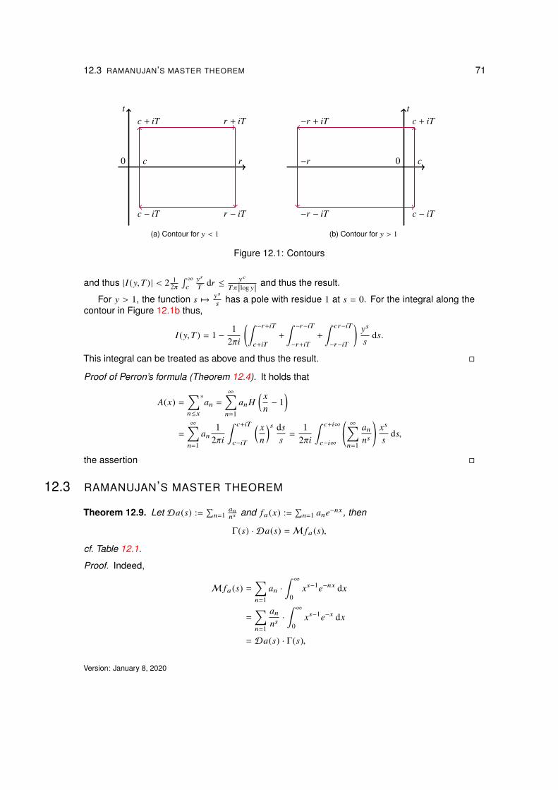
12.3 RAMANUJAN’S MASTER THEOREM 71

0

t

c r

r + iT

r − iT

c + iT

c − iT

(a) Contour for y < 1

0

t

c−r

−r + iT

−r − iT

c + iT

c − iT

(b) Contour for y > 1

Figure 12.1: Contours

and thus |I (y,T ) | < 2 12π´ ∞c

yr

T dr ≤ yc

Tπ |log y |and thus the result.

For y > 1, the function s 7→ ys

s has a pole with residue 1 at s = 0. For the integral along thecontour in Figure 12.1b thus,

I (y,T ) = 1 −1

2πi

(ˆ −r+iTc+iT

+

ˆ −r−iT−r+iT

+

ˆ cr−iT

−r−iT

)ys

sds.

This integral can be treated as above and thus the result.

Proof of Perron’s formula (Theorem 12.4). It holds that

A(x) =∑n≤x

∗an =

∞∑n=1

anH( x

n− 1

)=

∞∑n=1

an1

2πi

ˆ c+iT

c−iT

( xn

)s dss=

12πi

ˆ c+i∞

c−i∞

*,

∞∑n=1

an

ns+-

xs

sds,

the assertion

12.3 RAMANUJAN’S MASTER THEOREM

Theorem 12.9. Let Da(s) :=∑

n=1an

ns and fa (x) :=∑

n=1 ane−nx , then

Γ(s) · Da(s) =M fa (s),

cf. Table 12.1.

Proof. Indeed,

M fa (s) =∑n=1

an ·

ˆ ∞0

xs−1e−nx dx

=∑n=1

an

ns·

ˆ ∞0

xs−1e−x dx

= Da(s) · Γ(s),


72 MELLIN TRANSFORM

the assertion.

Perron’s formula6 describes the inverse Mellin transform applied to a Dirichlet series.

Theorem 12.10 (Ramanujan’s master theorem7). Suppose that φ is entire and |φ(s)Γ(s) | < 1R1+ε

ins : =(s) < c, |s | ≥ R

for increasing R. Then the Mellin transform of

f (x) :=∑k=0

φ(k)k!

(−x)k

isM f (s) =

ˆ ∞0

xs−1 f (x) dx = Γ(s) · φ(−s). (12.6)

The identity is often employed as formal identity.

Proof. The Gamma function s 7→ Γ(s) has poles at s ∈ −k : k = 0, 1, 2, . . . and the residues ats = −k are given by Γ(s) = (−1)k

k!(s+k) + O(1), cf. (6.6). By Cauchy’s residue theorem, applied to thecontour Figure 12.1b displays,

12πi

ˆ c+i∞

c−i∞

Γ(s)φ(−s)x−s ds =∑k=0

(−1)k

k!φ(k)xk =

∑k=0

φ(k)k!

(−x)k = f (x),

and the assertion follows by Mellin inversion (12.1).

12.4 CONVOLUTIONS

Definition 12.11 (Multiplicative convolution). The convolution of two functions f , g : (0,∞) → Cis

( f ∗ g)(x) =ˆ ∞

0f(

xy

)g(y)

dyy.

Proposition 12.12 (Convolution). It holds that

M ( f ∗ g) =M f · Mg; (12.7)

and further (cf. Table 12.1),

M

(xαˆ ∞

0yβ f

(xy

)g(y)

dyy

)(s) =M f (s + α) · Mg(s + α + β), (12.8)

M

(xαˆ ∞

0yβ f (xy)g(y)

dyy

)(s) =M f (s + α) · Mg(β − s − α). (12.9)

Proof. With Fubini,

M

(xαˆ ∞

0yβ f

(xy

)g(y)

dyy

)(s) =

ˆ ∞0

xs+α−1ˆ ∞

0yβ−1 f

(xy

)g(y) dydx

=x←xy

ˆ ∞0

yβ+s+α−1g(y) dy ·ˆ ∞

0xs+α−1 f (x) dx

=M f (s + α) · Mg(β + s + α)

6Oskar Perron, 1880–1975, German7Srinivasa Ramanujan, 1887–1920, Indian


12.4 CONVOLUTIONS 73

and thus (12.8) and (12.7). Further,

M

(xαˆ ∞

0yβ f (xy)g(y)

dyy

)(s) =

ˆ ∞0

xs+α−1ˆ ∞

0yβ−1 f (xy) g(y) dydx

=x←x/y

ˆ ∞0

xs+α−1 f (x) dx ·ˆ ∞

0yβ−s−α−1g(y) dy

=M f (s + α) · Mg(β − α − s)

and thus (12.9).

Proposition 12.13. We have that

M ( f · g)(s) =1

2πi

ˆ c+i∞

c−i∞

M f (z) · Mg(s − z) dz.

Proof. Recall from Table 12.1 thatM−11(·) = δ(· − 1), thus

12πi

ˆ c+i∞

c−i∞

M f (z) · Mg(s − z) dz =1

2πi

ˆ c+i∞

c−i∞

ˆ ∞0

xz−1 f (x) dx ·ˆ ∞

0ys−z−1g(y) dydz

=

ˆ ∞0

ˆ ∞0

12πi

ˆ c+i∞

c−i∞

(y

x

)−zdz︸︷︷︸

M−11(y/x)

f (x)x

dx g(y)ys−1 dy

=(12.1)

ˆ ∞0

ˆ ∞0

δ(y

x− 1

) f (x)x

dx ys−1g(y) dy

=y←xy

ˆ ∞0

ˆ ∞0

δ (y − 1) g(xy)ys−1 dy xs−1 f (x) dx

=

ˆ ∞0

g(x)xs−1 f (x) dx

=M ( f · g)(s)


Example 12.14. Let φ(k) = 1, then f (x) = e−x andM f (s) = Γ(s).

Example 12.15. Let φ(k) := −αk sin kπ2 so that

f (x) =∑k=0

φ(k)k!

(−x)k =∑n=0

(−1)nα2n+1

(2n + 1)!x2n+1 = sin αx.

It follows thatM (sin αx)(s) = Γ(s)αs sin sπ

2 (cf. Talbe 12.1).

Example 12.16. Let φ(k) := αk cos kπ2 so that

f (x) =∑k=0

φ(k)k!

(−x)k =∑n=0

(−1)nα2n

(2n)!(−x)2n = cos αx

and thusM (cos αx)(s) = Γ(s)αs cos sπ

2 .


74 MELLIN TRANSFORM

(a) Godfrey Harold Hardy, 1877–1947 (b) Srinivasa Ramanujan, 1887–1920: the manwho knew infinity

Figure 12.2: I remember once going to see him (Ramanujan) when he was lying ill at Putney.I had ridden in taxi-cab No. 1729, and remarked that the number seemed to be rather a dullone, and that I hoped it was not an unfavourable omen. ‘No’, he replied, ‘it is a very interestingnumber; it is the smallest number expressible as the sum of two [positive] cubes in two differentways.’


https://www.youtube.com/watch?v=oXGm9Vlfx4w

https://www.youtube.com/watch?v=oXGm9Vlfx4w

13Riemann zeta function

Mathematicians have tried in vain to thisday to discover some order in thesequence of prime numbers, and we havereason to believe that it is a mystery intowhich the human mind will never penetrate.

Leonhard Euler, 1707–1783

Riemann1 (cf. Riemann [15]) was the first to consider the function ζ on the complex plane.

Remark 13.1 (Derivatives). The derivatives of the zeta function are ζ (k) (s) = (−1)k∑∞

n=2logk nns ,

k ≥ 1.

Proposition 13.2 (Explicit values). For n = 1, 2, . . . it holds that

ζ (2n) = (−1)n−1 B2n2 (2n)!

(2π)2n. (13.1)

Proof. Choose x = 0 in the Fourier series (5.10) and note that βk is continuous for k ≥ 2 withβk (0) = Bk .

Example 13.3 (Basel problem). In particular we find the relations

ζ (2) =∑k=1

1k2 =

π2

6, ζ (4) =

∑k=1

1k4 =

π4

90, ζ (6) =

∑k=1

1k6 =

π6

945, (13.2)

etc.

Note that 1ns

=1nσ for s = σ + it so that (9.5) converges indeed for <(s) > 1. The following

provides an extension to <(s) > 0.

13.1 RELATED DIRICHLET SERIES

Lemma 13.4. It holds that

ζ (s) =1

1 − 21−s

∑n=1

(−1)n−1

ns, <(s) > 0. (13.3)

Remark 13.5. Note, that the abscissa of convergence (cf. Theorem 11.7) of the series∑

n=1(−1)n−1

ns

is σ0 = 0, although(1 − 21−s

)ζ (s) =

∑n=1

(−1)n−1

ns does not have a singularity at <(s) = s0. Thisis a notable difference to power series.

1Bernhard Riemann, 1826–1866, German

75

76 RIEMANN ZETA FUNCTION

Proof. Indeed,2

η(s) :=(1 −

22s

)ζ (s) = 1 +

12s+

13s+

14s+

15s+

16s+

17s+

18s+ . . .

−22s

−24s

−26s

−28s

= 1 −12s+

13s−

14s+

15s−

16s+

17s∓ . . .



ζ (s) =1

s − 1

∞∑n=1

(n

(n + 1)s−

n − sns

), (13.4)

the series converges for <(s) > 0.

Proof. Indeed,

∑n=1

(n

(n + 1)s−

n − sns

)=

∑n=1

n − 1ns−

∑n=1

n − sns

=∑n=1

n − 1 − n + sns

= (s − 1)ζ (s),

hence the identity. As for convergence recall that (1 + x)s =∑

k=0(sk

)xk . Thus

n(n + 1)s

−n − s

ns=

1ns

(n(1 +

1n

)−s− n + s

)=

1ns

(n − n

sn+ n

s(s + 1)2n2 + O

(1n2

)− n + s

)=

s(s + 1)2ns+1 + O

(1

ns+2

)and thus the result.

Remark 13.7. The series converges for s = 1 to∑

n=1(

nn+1 −

n−1n

)=

∑n=1

(− 1

n+1 +1n

)= 1 so that

ζ has a pole at s = 1 with residue 1, i.e., ζ (s) = 1s−1 + O(1).

Proposition 13.8. The series

ζ (s) =1

s − 1

∞∑n=1

n(n + 1)2

(2n + 3 + s(n + 1)s+2 −

2n − 1 − sns+2

)

converges for <(s) > −1.

2The function η is also known as Dirichlet eta function.


13.2 REPRESENTATIONS AS INTEGRAL 77

Proof. As above,∑n=1

n(n + 1)2

(2n + 3 + s(n + 1)s+2 −

2n − 1 − sns+2

)=

∑n=1

(n − 1)n2

·2(n − 1) + 3 + s

ns+2 −n(n + 1)

2·

2n − 1 − sns+2

=∑n=1

2n2(s − 1)2ns+2 = (s − 1) ζ (s),

after simplifications. Convergence can be established as above, it holds that

n(n + 1)2

(2n + 3 + s(n + 1)s+2 −

2n − 1 − sns+2

)=

12ns+2

(s + 3

3

)+ O

(n−s−3

)and thus the assertion.

Remark 13.9. Note that3

ζ (0) = −12

∞∑n=1

(n

2n + 3n + 1

− (n + 1)2n − 1

n

)= −

12

∞∑n=1

(1n−

1n + 1

)= −

12.

13.2 REPRESENTATIONS AS INTEGRAL

Proposition 13.10 (Mellin transform). It holds that

ζ (s) Γ(s) =ˆ ∞

0

xs−1

ex − 1dx (<(s) > 1). (13.5)

Proof. Apply Theorem 12.9 with f (x) =∑

n=1 e−nx = 1ex−1 .

Theorem 13.11. It holds that

ζ (s) = sˆ ∞

1

bucus+1 du, <(s) > 1. (13.6)

Proof. Choose an := 1 so that A(x) = bxc and φ(x) = 1xs . Then apply Abel’s summation

formula (8.6).


ζ (s) = −sˆ ∞

0frac

(1t

)ts−1 dt, 0 < <(s) < 1 (13.7)

where frac(x) := x − bxc is the fractional part of the number x ∈ R.

Proof. From (13.6) we infer that

ζ (s) = sˆ 1

0

⌊1u

⌋us−1 du, <(s) > 1.

3I.e., 1 + 1 + 1 + · · · = − 12,cf. Figure 13.3



It holds that´ 1

01uus−1 du =

´ 10 us−2 du = us−1

s−11

u=0= 1

s−1 for <(s) > 1 and thus

ζ (s) −s

s − 1= sˆ 1

0

(⌊1u

⌋−

1u

)us−1 du. (13.8)

Now note that´ ∞

11uus−1 du =

´ ∞1 us−2 du = us−1

s−1∞

u=1= − 1

s−1 for <(s) < 1 and thus

ζ (s) −s

s − 1= sˆ ∞

0

(⌊1u

⌋−

1u

)us−1 du + s

ˆ ∞1

1u

us−1 du.

= sˆ ∞

0

(⌊1u

⌋−

1u

)us−1 du −

ss − 1


Remark 13.13. The equation (13.8) holds for<(s) > 0 and thus proves that ζ has a single poleat s = 1.

Definition 13.14. The function M (x) :=∑

n≤x µ(n) is the Mertens function.4


1ζ (s)

= sˆ ∞

1

M (u)us+1 du, <(s) > 1. (13.9)

Proof. In Abel’s summation formula (8.6) choose an := µ(n) so that A(x) = M (x) and φ(x) = 1xs ,

then the result derives from (9.9).

Theorem 13.16 (Riemann, cf. Edwards [7]). It holds that (recall that (−x)s = exp(s · log(−x)

),

which is not defined for x ∈ R≥0)

2 sin(πs) Γ(s) ζ (s) = i˛H

(−x)s−1

ex − 1dx, (13.10)

where H is the Hankel5 contour.

Remark 13.17. The Hankel contour (aka. keyhole contour, cf. Figure 13.1) is a path in thecomplex plane which extends from [+∞, δ], around the origin counter clockwise and back to[+∞,−δ], where δ is an arbitrarily small positive number.

Proof. We have that ˛H

(−x)s−1

ex − 1dx = −

(ˆ δ

+∞

+

ˆ|x |=δ+

ˆ ∞δ

)(−x)s dx(ex − 1)x

, (13.11)

although, strictly speaking, the path of integration must be taken to be slightly above the realaxis as it descends from +∞ to 0 and slightly below the real axis as it goes from 0 back to +∞.

Now note thatˆ|x |=δ

(−x)s dx(ex − 1)x

=

ˆ|x |=δ

xs−2∞∑k=0

Bk(−x)k

k!dx

=

ˆ 2π

0δs−1 · eit (s−1)

∞∑k=0

(−1)kBkδkeikt

k!dt −−−−→

δ→00

4Franz Mertens, 1840–19275Hermann Hankel, 1839–1873, German mathematician


13.3 GLOBALLY CONVERGENT SERIES 79

0

Figure 13.1: Hankel contour

-15 -10 -5 5

-4

-3

-2

-1

1

2

3

(a) reals

-14 -12 -10 -8 -6 -4 -2

-0.10

-0.05

0.05

0.10

(b) negative reals

Figure 13.2: ζ on the real line

for s > 1 by (5.1). The remaining terms in the integral (13.11) are

limδ→0

ˆ δ

+∞

exp(s log x − iπ)(ex − 1)x

dx +ˆ +∞δ

exp(s log x + iπ)(ex − 1)x

dx =(eiπs − e−iπs

) ˆ ∞0

xs−1

ex − 1dx.

With (13.5) we thus have¸H

(−x)s−1

ex−1 dx = −2i sin(πs)Γ(s)ζ (s) and thus the assertion.

13.3 GLOBALLY CONVERGENT SERIES


ζ (s) =1

1 − 21−s

∑n=0

12n+1

n∑k=0

(−1)k(nk

)1

(k + 1)s,

the series converges for all s ∈ C.

Proof. Apply Euler transform (cf. (8.2)) to (13.3).

Theorem 13.19 (Cf. Hasse [11]). It holds that

ζ (s) =1

s − 1

∑n=0

1n + 1

n∑k=0

(nk

)(−1)k

(k + 1)s−1 ; (13.12)



Figure 13.3: Ramanujan’s proof of ζ (−1) = 1 + 2 + 3 + · · · = − 112 in his letter to Hardy

the series converges for all s ∈ C.

Proof. Note first that 1ks =

1Γ(s)

´ ∞0 e−kt ts−1 dt and

n∑k=0

(nk

)(−1)k

(k + 1)s=

1Γ(s)

ˆ ∞0

n∑k=0

(−1)k(nk

)e−(k+1)t ts−1 dt

=1Γ(s)

ˆ ∞0

(1 − e−t

)ne−t ts−1 dt.

Finally, as log(1 − x) = −∑

n=0xn+1

n+1 ,∑n=0

1n + 1

n∑k=0

(nk

)(−1)k

(k + 1)s=

1Γ(s)

ˆ ∞0

∞∑n=0

(1 − e−t

)nn + 1

e−t ts−1 dt

=1Γ(s)

ˆ ∞0

t1 − e−t

e−t ts−1 dt

=1Γ(s)

ˆ ∞0

ts

et − 1dt

=1Γ(s)

ζ (s + 1) Γ(s + 1)

by (13.5) and thus the result.

Corollary 13.20 (Explicit values, cf. Remark 13.9). It holds that ζ (0) = − 12 and

ζ (−n) = −Bn+1n + 1

, n = 1, 2, 3, . . . .

Proof. By comparing (5.5) and (13.12) it follows with (5.6) that ζ (−n) = −Bn+1 (1)n+1 = −

Bn+1n+1 .

Alternative proof. The assertion follows as well from the residue theorem with (5.1) and (13.10).

Remark 13.21 (Cf. Figure 13.3). This result is often stated as 1 + 1 + 1 + · · · = ζ (0) = − 12 or

1 + 2 + 3 + · · · = ζ (−1) = − 112 .

Corollary 13.22. It holds (cf. Remark 5.3 and Figure 13.2) that

ζ (s) = 0, s = −2,−4,−6, . . .

These are called the trivial zeros of the Riemann zeta function.


13.4 POWER SERIES EXPANSIONS 81

13.4 POWER SERIES EXPANSIONS

Define the function fn(s) := n(n+1)s −

n−sns and recall from (13.4) that ζ (s) = 1

s−1∑∞

n=1 fn(s). Theseries converges for <(s) > 0. From Taylor we obtain that

ζ (s) =1

s − 1

∑n=1

(fn(1) + (s − 1) f ′n(1) +

(s − 1)2

2f ′′n (1) + . . .

)=

∑n=1 fn(1)s − 1

+∑n=1

f ′n(1) +s − 1

2

∑n=1

f ′′n (1) + . . .

Now note, for k ≥ 1, that

(−1)k f (k)n (s) = −k

logk−1 nns

−(n − s) logk n

ns+

n logk (n + 1)(n + 1)s

and

(−1)k f (k+1)n (1)

k + 1=

logk nn−

1k + 1

(n

n + 1logk+1(n + 1) −

n − 1n

logk+1 n). (13.13)

Definition 13.23. The numbers

γk := limm→∞

m∑n=1

logk nn−

logk+1 mk + 1

(13.14)

are Stieltjes constants.6

Remark 13.24. The constant γ0 = γ = 0.577 215 . . . is Euler’s constant or Euler–Mascheroniconstant, cf. (7.3). The following constants are γ1 = −0.072 815 . . . , γ2 = −0.009 690 . . . , etc.

Remark 13.25. Note in (13.14) that´ m

1logk n

n dn = logk+1 mk+1 .

Theorem (Global Laurent series expansion). It holds that

ζ (s) =1

s − 1+

∞∑k=0

(−1)kγkk!

(s − 1)k (13.15)

=1

s − 1+ γ − γ1(s − 1) +

γ22

(s − 1)2 ∓ . . . ,

for every s ∈ C\0, where γk are Stieltjes constants. ζ has a simple pole at s = 1 with residueRes1(ζ ) = 1.

Proof. Note first that ∑n=1

fn(1) =∑n=1

1n(n + 1)

= 1

It follows with (13.13) that

γk = limm→∞

m∑n=1

logk nn−

mm + 1

logk+1(m + 1)k + 1

= limm→∞

m∑n=1

(−1)k f (k+1)n (1)

k + 1,

6Thomas Jean Stieltjes, 1856–1894, Dutch



as the sum is telescoping.Note further that

mm + 1

logk+1(m + 1) − logk+1 m =m

m + 1

(log m + log

(1 +

1m

))k+1− logk+1 m

=m

m + 1

(log m +

1m

)k+1− logk+1 m + O

(logk m

m

)= −

1m + 1

logk+1 m + O(logk m

m

)−−−−−→m→∞

0


13.5 EULER’S THEOREM

Corollary 13.26 (Euler’s theorem). The series of reciprocal primes diverges,∑p prime

1p= ∞.

Remark 13.27 (Euler’s informal proof). We provide Euler’s informal proof first. Note, that

log∑n=1

1n= log

∏p prime

11 − p−1 = −

∑p prime

log(1 −

1p

)

=∑

p prime

(1p+

12p2 +

13p3 + . . .

)=

∑p prime

1p+

12

∑p prime

1p2 +

12

∑p prime

1p2 + . . .

= A +12

B +13

C +13

D + . . .

= A + K

for some K < 1. By letting x → 1 in log 11−x =

∑n=1

xn

n we find that∑

n=11n = log∞. It follows that

A =∑

p prime1p = log log∞.

Proof. From (9.15) and Proposition 9.32 we deduce that

log ζ (s) −

∑p prime

1ps

≤

∑k=2

1k

1k − 1

= 1.

From Taylor series expansion (13.15) we have for s ∼ 1 and <(s) > 1 that

P(s) =∑

p prime

1ps∼ log ζ (s) ∼ log

1s − 1

(13.16)



13.6 THE FUNCTIONAL EQUATION 83

Figure 13.4: Riemann, 1859

Remark 13.28. Note the contrast: it holds that∑p prime

1ps∼ log

1s − 1

by (13.16), but, as ζ ′(s)ζ (s) = −

1s−1 , ∑

p prime

log pps∼

1s − 1

by (9.13).

Theorem 13.29 (Mertens’ second theorem). It holds that

∑p≤x

1p∼ log log x + γ +

∑k=2

µ(k)k

log ζ (k) + O(

1log x

).

The Meissel–Mertens constant is M := γ +∑

k=2µ(k)k log ζ (k) = γ +

∑p∈P log

(1 − 1

p

)+ 1

p ≈

0.21649....

See Theorem 16.9 below for a proof based on the prime number theorem (PNT, Theo-rem 16.4 below).

Remark 13.30. We have that log log 1010 000 ≈ 10.04 and the age of the universe is ≈ 4.3 × 1017

seconds.

13.6 THE FUNCTIONAL EQUATION

Riemann’s functional equation for the ζ-function is a reflection formula relating ζ (s) with ζ (1− s).



Theorem 13.31 (Functional equation). It holds that

ζ (s) = 2(2π)s−1 sinπs2Γ(1 − s) ζ (1 − s).

Further, with ξ (s) := s(s−1)2 πs/2 Γ

( s2)ζ (s) we have that

ξ (s) = ξ (1 − s). (13.17)

Remark 13.32. Riemann actually considered the function Ξ(z) := ξ(

12 + iz

).

Proof. Recall from (8.8) the definition of the Jacobi theta function ϑ and define

ψ(x) :=32

x ϑ′(x) + x2 ϑ′′(x) =∑k=1

(2(k2πx

)2− 3k2πx

)e−k

2πx (13.18)

(see Figure 13.5a for the graph; cf. Riemann’s note, Figure 13.4). As Jacobi’s theta function, thefunction ψ satisfies the functional equation (cf. (8.9))

ψ(x) =1√

xψ

(1x

). (13.19)

Indeed, we have from (13.18) that

ψ(x) =√

xddx

(x3/2 ϑ′(x)

)=√

xddx

(x3/2 d

dxϑ(x)

)

and with (8.9) thus

ψ(x) =√

xddx

(x3/2 d

dx

(x−1/2 ϑ

(1x

)))=√

xddx

(x3/2

(−

12

x−3/2 ϑ

(1x

)− x−5/2 ϑ′

(1x

)))=√

xddx

(−

12ϑ

(1x

)−

1xϑ′

(1x

))=√

x(

12x2 ϑ

′

(1x

)+

1x2 ϑ

′

(1x

)+

1x3 ϑ

′′

(1x

))=

1√

x

(32

1xϑ′

(1x

)+

1x2 ϑ

′′

(1x

))=

1√

xψ

(1x

),

i.e., (13.19).


13.6 THE FUNCTIONAL EQUATION 85

It holds that ˆ ∞0

xs2 −1 ψ(x) dx =

∑k=1

ˆ ∞0

xs2 −1

(2(k2π x

)2− 3k2π x

)e−k

2πx dx

=x← x

k2π

∑k=1

ˆ ∞0

xs2 −1(

k2π) s

2

(2x2 − 3x

)e−x dx

=ζ (s)πs/2

(2 Γ

( s2+ 2

)− 3 Γ

( s2+ 1

))=ζ (s)πs/2Γ

( s2

) (2

s2

( s2+ 1

)− 3

s2

)=ζ (s)πs/2

s(s − 1)2

Γ

( s2

).

Hence (cf. Table 12.1)

ξ (s) =ζ (s)πs/2

s(s − 1)2

Γ

( s2

)=

ˆ ∞0

xs2 −1 ψ(x) dx (13.20)

=

ˆ ∞0

xs2 −

32 ψ

(1x

)dx

=x←1/x

ˆ ∞0

x−s2 +

32−2 ψ (x) dx

=

ˆ ∞0

x1−s

2 −1 ψ (x) dx;

comparing with (13.20) reveals that ξ is symmetric and thus the functional equation (13.17).However, convergence remains to be discussed. To this end observe that (13.18) implies

that ψ (k) (x) → 0 as x → ∞ for every k = 0, 1, . . . and further, ψ (k) (x) → 0 as x → 0 by (13.19). Itfollows that (13.19) holds for all s ∈ C, the integral converges globally.

Remark 13.33 (Fourier transform). With (13.20) we have that

ξ (s) =ˆ ∞

0x

s2 −1 ψ(x) dx =

ˆ ∞0

xs−1 · 2ψ(x2) dx (13.21)

=

ˆ ∞−∞

ex (s−1/2) · 2 ex/2ψ(e2x ) dx

=

ˆ ∞−∞

cos *,

s − 12

ix+

-· 2ex/2 ψ

(e2x ) dx,

where x 7→ 2 ex/2 ψ(e2x ) is symmetric.

Remark 13.34 (Representations of cos t x). The Fourier transform of the following representa-tions derives from (6.8):

cos t x =sin πtπt−

sin πtπ

∑k=1

(−1)k2t

k2 + t2 cos k x (−π ≤ x ≤ π)

= limn→∞

H2n

(t x

2√

n

)(all x)

= Tt (cos x) = cosπx2+ t

∑j=1

(2x) j

jcos

π(t − j)2

( t+j−22

j − 1

);



0.5 1.0 1.5 2.0 2.5

0.2

0.4

0.6

0.8

(a) Graph of 2ψ(x2), see (13.18)

20 40 60 80 100

-4

-2

2

4

(b) Riemann–Siegel Z

Figure 13.5: Function plots

Hn is the Hermite polynomial and Tt the generalized Chebyshev polynomial.

Remark 13.35 (Riemann–Siegel theta function, Z-function). To investigate the function ζ on the

critical lines ∈ C : <(s) = 1

2

it is convenient to define θ(t) := arg Γ

( 12+it

2

)− t log π

2 (the principal

branch of the function ξ) and Z (t) := eiθ (t)ζ(

12 + it

). Note, that Z (t) ∈ R and ζ

(12 + it

) = ±Z (t)for t ∈ R. Figure 13.5b displays the graph of Z.

Proposition 13.36 (Explicit values). It holds that ζ ′(0) = − 12 log 2π and ζ ′(−2n) = (−1)nζ (2n+1)(2n)!

22n+1π2n .

We give a further proof of the functional equation.

Second proof of Theorem 13.31. Recall from (13.6) that ζ (s) = s´ ∞

1bxcxs+1 dx, thus

ζ (s) =1

s − 1+

12− sˆ ∞

1

x − bxc − 12

xs+1 dx (<(s) > −1)

= −sˆ ∞

0

x − bxc − 12

xs+1 dx (−1 < <(s) < 0).

Now recall the sawtooth wave from (5.11) so that

ζ (s) =sπ

∞∑n=1

1n

ˆ ∞0

sin 2πnxxs+1 dx

=sπ

∑n=1

(2nπ)s

n

ˆ ∞0

sin xxs+1 dx

=sπ

(2π)sζ (1 − s)(− Γ(−s)

)sin

πs2,

and thus the result. We have used here´ ∞

0 xs−1 sin x dx = Γ(s) sin πs2 , see Example 12.15 and

Table 12.1.


13.7 RIEMANN HYPOTHESIS (RH) 87

13.7 RIEMANN HYPOTHESIS (RH)

The first non-trivial, or ’non-obvious’ zeros of the Riemann zeta are (cf. Figure 13.5b)

ρ1 := 1/2 + i · 14.134 725 141 734 693 790 . . .,

ρ2 := 1/2 + i · 21.022 039 638 771 554 993 . . .,

ρ3 := 1/2 + i · 25.010 857 580 145 688 763 . . . andρ4 := 1/2 + i · 30.424 876 125 859 513 210 . . ..

The following formulation of the Riemann hypothesis (RH) quotes the second millenniumproblem, http://www.claymath.org/millennium-problems :

The prime number theorem determines the average distribution of the primes. TheRiemann hypothesis tells us about the deviation from the average. Formulated inRiemann’s 1859 paper, it asserts that all the ’non-obvious’ zeros of the zeta functionare complex numbers with real part 1/2.

13.8 HADAMARD PRODUCT

Hadamards7 product follows from Weierstrass8 product theorem.


ζ (s) =e(log(2π)−1− γ2 )s

2(s − 1)Γ(1 + s

2

) ∏ρ

(1 −

sρ

)e

sρ ,

where the product is over the non-trivial zeros ρ of ζ and the γ again is the Euler–Mascheroniconstant.

Corollary 13.38. It holds that

ζ ′(s)ζ (s)

= log 2π −γ

2− 1 −

1s − 1

−12Γ′(s/2 + 1)Γ(s/2 + 1)

+∑ρ

(1

s − ρ+

1ρ

),

where the sum is among all nontrivial zeros ρ of the Riemann zeta function.


ξ (s) =12

∏ρ

(1 −

sρ

).

Theorem 13.40 (Li’s criterion). It holds thatddz

log ξ( z

z − 1

)=

∑n=1

λn+1zn,

where λn := 1(n−1)!

dndsn

(sn−1ξ (s)

) s=1=

∑ρ 1 −

(1 − 1

ρ

)n.

The Riemann hypothesis is true iff λn > 0 for all n = 1, 2, . . .

PROBLEMS

Exercise 13.1. Verify the identity (13.18).

7Jacques Hadamard, 1865–1963, French8Karl Weierstraß, 1815–1897, German


http://www.claymath.org/millennium-problems



14Further results and auxiliary relations

14.1 OCCURRENCE OF COPRIMES

Theorem 14.1. The probability of two numbers being coprime is 6π2 ≈ 60.8%; more precisely:

letcopr(x) := (m, n) ∈ N × N : m, n ≤ x and m and n are coprime.

Then

limx→∞

copr(x)x2 =

6π2 .

Proof. DefineAk (x) :=

(m, n) ∈ N2 : m, n ≤ x and gcd(m, n) = k

and A(x) :=⋃

k≤x Ak (x), the union of disjoint sets. Note that, for x and k fixed, the map

copr( x

k

)→ Ak (x)

(m, n) 7→ (k · m, k · n)

is a bijection. Therefore, bxc2 =∑

k≤x |Ak (x) | =∑

k≤xcopr

(xk

) and by Corollary 10.13 thuscopr (x) =

∑k≤x µ(k)

⌊xk

⌋2.

Now note that(xk

)2−

⌊xk

⌋2≤ 2 x

k . Hence

copr (x) −

∑k≤x

µ(k)( x

k

)2≤ 2x

∑k≤x

1k≤ 2x(1 + log x)

or

copr (x)x2 −

∑k≤x

µ(k)k2

≤ 2

1 + log xx

. (14.1)

With (9.9) and (13.2) we find that∑∞

k=1µ(k)k2 =

1ζ (2) =

6π2 . The result follows by letting x → ∞

in (14.1).

14.2 EXPONENTIAL INTEGRAL

Definition 14.2. The exponential integral is

Ei(z) := p.v.ˆ z

−∞

et

tdt,

where p.v. denotes the Cauchy principal value.

89

90 FURTHER RESULTS AND AUXILIARY RELATIONS


Ei(z) = γ + log z +∞∑k=1

zk

k · k!. (14.2)

Proof. By integration by parts, (6.5) and (6.1),

log ε +ˆ ∞ε

e−t

tdt =

(1 − e−ε

)log ε +

ˆ ∞ε

e−t log t dt −−−−→ε→0

ˆ ∞0

e−t log t dt = Γ′(1) = −γ.

It follows that

Ei(z) ←−−−−ε→0

ˆ −ε−∞

et

tdt − log ε + log z +

ˆ z

ε

et − 1t

dt −−−−→ε→0

γ + log z +∞∑k=1

ˆ z

0

tk−1

k!dt


14.3 LOGARITHMIC INTEGRAL FUNCTION

Definition 14.4. The logarithmic integral is

li(x) := p.v.ˆ x

0

1log t

dt,

for x > 1 being the Cauchy principal value.

Proposition 14.5. It holds that li z = Ei(log z) = γ + log log z +∑∞

k=1logk zk ·k! .

Asymptotic expansion. The logarithmic integral has the asymptotic series expansion

li(x) =x

log x

(1 +

1log x

+2

log2 x+ · · · +

k!logk x

)+ O

(x

logk+1 x

)(14.3)

as x → ∞. To see this asymptotic expansion replace x ← ey, then

li(ey

)=

ˆ ey

0

1log t

dt =t←ey (1−t )

eyˆ ∞

0

e−yt

1 − tdt .

By Taylor series expansion we have 11−t = 1 + t + · · · + tn−1 + tn

1−t , thus

li(ey

)= ey

n∑k=1

ˆ ∞0

tk−1e−yt dt + eyˆ ∞

0

e−yt tn

1 − tdt

= eyn∑

k=1

(k − 1)!yk

+ Rn(y),

where Rn(y) = ey´ ∞

0e−yt tn

1−t dt = O(1/yn+1

)as y → ∞. The expansion follows by replacing

y ← log x again.More generally and by a similar reasoning it can be shown thatˆ x

2

dt

logk t=

x

logk x

(1 +

klog x

+(k + 1)k

log2 x+ · · · +

(k + ` − 1

`

)`!

log` x

)+ O

(x

logk+`+1 x

), (14.4)

as x → ∞.


14.4 ANALYTIC EXTENSIONS 91

Remark 14.6. Differentiate (14.4) with respect to x to see the identity.

Remark 14.7. Compare with (14.3) and Gauß’ letter (Figure 1.1, second page) the extension

xlog x − 1

=x

log x(1 − 1

log x

) = xlog x

(1 +

1log x

+1

log2 x+ . . .

).

14.4 ANALYTIC EXTENSIONS

The following is from Zagier [22].

Theorem 14.8 (Analytic theorem, Newman [14]). Let f (t) (t ≥ 0) be bounded and locally inte-grable function and suppose that the function g(z) :=

´ ∞0 f (t)e−z t dt (<(z) > 0) extends holo-

morphically to <(z) ≥ 0. Then´ ∞

0 f (t) dt exists and equals g(0).

Proof. For T > 0 set gT (z) :=´ T

0 f (t)e−z t dt. The function gT is holomorphic for all z ∈ C. To

prove the theorem we have to show that limT→∞ gT (0) = g(0).Let R > 0 be large and C the boundary of the region

z ∈ C : |z | ≤ R, <(z) ≥ −δ

, where δ > 0

is small enough (depending on R) so that g is holomorphic in and on C. By Cauchy’s theorem,

g(0) − gT (0) =1

2πi

˛C

(g(z) − gT (z)

)ezT

(1 +

z2

R2

)1z

dz. (14.5)

(i) Note that for z ∈ C+ :=z ∈ C : |z | = R and <(z) > 0

,

|g(z) − gT (z) | =

ˆ ∞T

f (t)e−zt dt≤ Bˆ ∞T

e−zt dt = B

e−T <(z)

<(z)

and further(1 + z2

R2

)1z =

1z +

zR2 =

zR2 +

zR2 =

2<(z)R2 , thus

ez T

(1 +

z2

R2

)1z

≤ eT <(z) 2<(z)

R2 .

Consequently, on C+, the integrand in (14.5) is bounded by 2BR2 .

(ii) Now consider z ∈ C− :=z ∈ C : |z | = R and <(z) < 0

.

(a) The function gT is an entire function (i.e., analytic everywhere) and the contour C− inthe integral (14.5) thus may be changed to z ∈ C, <(z) < 0 and |z | = R. It holds that

|gT (z) | =

ˆ T

0f (t) e−z t dt

≤ Bˆ T

−∞

e−z t dt = B

e−<(z)T

<(z)

so that the integrand in (14.5) thus again is bounded by 2BR2 .

(b) The remaining integrand in (14.5) is the function g(z)ezT(1 + z2

R2

)1z , which decreases

uniformly on the remaining contour (z ∈ C−, <(z) = −δ), as T increases. The totallength of the contour is 2πR, thus it follows that |g(0) − gT (0) | < 4B+1

R for T sufficientlylarge. The assertion follows, as R > 0 is arbitrary.


92 FURTHER RESULTS AND AUXILIARY RELATIONS


15Prime counting functions

15.1 RIEMANN PRIME COUNTING FUNCTIONS AND THEIR RELATION

Definition 15.1 (Prime-counting function). The prime-counting function is

π(x) :=∑p≤x,

p prime

1.

The Riemann prime-counting function is

J (x) :=∑k=1

π(x1/k )k

=∑pk ≤x,p prime

1k. (15.1)

Different notation in frequent use is also J = Π.

Note that π(2) = 1, π(4) = 2, J (4) = 2 12 and

π(pn) = n (15.2)

for the nth prime pn (n ∈ N). We also have that pπ (p) = p, if p is prime.

Remark 15.2. As π(x) = 0 for x < 2 it is sufficient in (15.1) to consider only x1/n ≥ 2 and to sum

up to n ≤ 1logx (2) = log2(x), i.e., J (x) =

∑log2 (x)n=1

π(x

1/n)

n .


π(x) =∑n=1

µ(n)n

J(x1/n

). (15.3)

Out[37]=

100 200 300 400 500

20

40

60

80

100

l i(n)

π(n)n

log(n)

Out[47]=

100 200 300 400 500

20

40

60

80

100

l i(n)

J(n)n

log(n)

Figure 15.1: Prime counting functions π and J

93

94 PRIME COUNTING FUNCTIONS

Proof. Indeed, with (15.1),∑d1=1

µ(d1)d1

J(x1/d1

)=

∑d1=1

µ(d1)d1

∑d2=1

1d2π

(x1/d1d2

)=

∑n=1

π(x1/n

) 1n

∑d1d2=n

µ(d1)

= π(x),

where we have employed (9.7) (the Dirichlet inverse of the Möbius function).

Theorem 15.4 (Mellin transforms). It holds that

log ζ (s) = sˆ ∞

0

π(x)x(xs − 1)

dx

= sˆ ∞

0

J (x)xs+1 dx

and (recall the zeta prime function P(s) =∑

p prime1ps from (9.14))

P(s) = sˆ ∞

0

π(x)xs+1 dx.

Proof. By Riemann–Stieltjes integration by parts

log ζ (s) = −∑p

log(1 −

1ps

)= −

ˆ ∞1

log(1 −

1xs

)dπ(x)

=

ˆ ∞1

π(x)s 1xs+1

1 − 1xs

dx

= sˆ ∞

0π(x)

1x(xs − 1)

dx;

a slightly more explicit derivation is

log ζ (s) = −∑p

log(1 −

1ps

)= −

∑n=2

(π(n) − π(n − 1)

)log

(1 −

1ns

)= −

∑n=2

π(n)(log

(1 −

1ns

)−

(1 −

1(n + 1)s

))

=∑n=2

π(n)ˆ n+1

n

sx(xs − 1)

dx

= sˆ ∞

2

π(x)x(xs − 1)

dx.


15.2 CHEBYSHEV PRIME COUNTING FUNCTIONS AND THEIR RELATION 95

Further

log ζ (s) = sˆ ∞

0

π(x)x(xs − 1)

dx

= sˆ ∞

0

π(x)xs+1

11 − x−s

dx

= sˆ ∞

0

π(x)xs+1 xs

∑k=1

x−sk dx

= s∑k=1

ˆ ∞0

π(x)x

x−sk dx

=x←x1/k

s∑k=1

ˆ ∞0

π(x1/k

)x1/k

x−s ·1k

x1/k−1 dx

= sˆ ∞

0

J (x)xs+1 dx

and thus the result.The Mellin transformation of P (cf. (9.14)) is immediate from

P(s) =ˆ ∞

1

1xs

dπ(x) = −ˆ ∞

1π(x) d

1xs=

ˆ ∞1

π(x)1

xs+1 dx.

Proposition 15.5. It holds that (cf. (9.11))

J (x) =∑n≤x

Λ(n)log n

. (15.4)

Proof. Indeed, J (x) =∑

pk ≤x1k =

∑pk ≤x

log p

log pk =∑

n≤xΛ(n)log n .

15.2 CHEBYSHEV PRIME COUNTING FUNCTIONS AND THEIR RELATION

Definition 15.6. The first Chebyshev 1 function is

ϑ(x) :=∑p≤x,

p prime

log p =π (x)∑k=1

log pk = log(x#), (15.5)

the second Chebyshev function is the summatory von Mangoldt function (cf. (9.11)),

ψ(x) :=∑n≤x

Λ(n) =∑pk ≤x,p prime

log p; (15.6)

the primorial isx# :=

∏p≤x,

p prime

p.

Remark 15.7. Note that n# = pπ (n)#.



Out[52]=

100 200 300 400 500

100

200

300

400

500

x

ϑ(x)

(a) Plot of ϑ

20000 40000 60000 80000 100000

-500

-400

-300

-200

-100

(b) Plot of ϑ(x) − x

Figure 15.2: Chebyshev function ϑ

Out[48]=

100 200 300 400 500

100

200

300

400

500

n

Ψ(n)

(a) Plot of ψ

20000 40000 60000 80000 100000

-150

-100

-50

50

100

150

(b) Plot of ψ(x) − x

Figure 15.3: Chebyshev function ψ


15.2 CHEBYSHEV PRIME COUNTING FUNCTIONS AND THEIR RELATION 97

Remark 15.8. Note that we expect that ϑ(x) ∼´ x

1 log p d(´ p

01

log t dt)=´ x

1log plog p dt = x − 1.


ψ(x) =∑p≤x

⌊log xlog p

⌋log p (15.7)

andψ(x) = ϑ(x) + ϑ

(x1/2

)+ ϑ

(x1/3

)+ · · · =

∑m=1

ϑ(x1/m

)and conversely,

ϑ(x) =∑m=1

µ(m) ψ(x1/m

).

Proof. Note that log xlog p = logp x.

Then ∑d1=1

µ(d1) ψ(x1/d1

)=

∑d1=1

µ(d1)∑d2=1

ϑ(x1/d1d2

)=

∑n=1

ϑ(x1/n

) ∑d1d2=n

µ(d1)

= ϑ(x),

where we have employed (9.7) (the Dirichlet inverse of the Möbius function; cf. Theorem 15.3).

Proposition 15.10. We have that

log n =∑d |n

Λ(d) and Λ(n) = −∑d |n

µ(d) log d.

Proof. Use Möbius inversion formula (10.5).

Proposition 15.11. It holds that (recall the definition of the zeta prime function (9.14))

−dds

P(s) =∑

p prime

log pps= sˆ ∞

1

ϑ(x)xs+1 dx

and further (cf. Theorem 9.29) we have

dds

log ζ (s) =ζ ′(s)ζ (s)

= −∑n=2

Λ(n)ns= −s

ˆ ∞1

ψ(x)xs+1 dx

and (cf. Proposition 9.28)

log ζ (s) =∑n=2

Λ(n)ns log n

.

1Pafnuty Chebyshev, 1821–1894, Russian



Proof. With −P′(s) =∑

p primelog pps (cf. (9.14)) we have that

∑p prime

log pps=

ˆ ∞1

dϑ(x)xs

= sˆ ∞

1

ϑ(x)xs+1 dx. (15.8)

From (9.6) (see also (9.29)) we deduce that

−ζ ′(s)ζ (s)

=dds

∑p prime

log(1 −

1ps

)= −

∑p prime

1ps log 1

p

1 − 1ps

=∑

p prime

∑k=1

log ppsk

=∑n=1

Λ(n)ns

and thus the first identity.The second identity follows from Abel’s summation formula (8.6), as the Chebyshev function

ψ is the summatory function of Λ by (15.6).

15.3 RELATION OF PRIME COUNTING FUNCTIONS

The extremely ingenious proof of the following proposition is due to Chebyshev.

Proposition 15.12 (Chebyshev). It holds that

ϑ(x) < x · log 4 (< 1.39 · x) (15.9)

for all x > 0.

Proof. Employing the primorial (15.5) the statement is equivalent to Fn := n# =∏

p≤n < 4n forall n ∈ N which we shall verify by induction.

The statement is true for n = 0, 1, 2 and 3.If n is even, then Fn = Fn−1 < 4n−1 < 4n, as desired.If n is odd, then n = 2k + 1. By induction hypothesis

∏p≤k+1 < 4k+1.

Consider the binomial coefficient(2k+1

k

)=

(2k+1) ·2k · · ·(k+2)1·2·3· · ·k . Clearly, for every prime p with

k + 2 ≤ p ≤ 2k + 1, one has that p |(2k+1

k

)and hence

∏k+1<p≤2k+1 p ≤

(2k+1k

)=

(2k+1k+1

)≤

12 (1 + 1)2k+1 = 4k . It follows that

Fn = F2k+1 =∏

p≤k+1p ·

∏k+1<p≤2k+1

p < 4k+1 ·

(2k + 1

k

)< 4k+1 4k = 42k+1 = 4n,

the assertion.

Theorem 15.13 (Prime counting functions). The prime counting functions are related as follows:

(i) π(x) = ϑ(x)log x +

´ x2

ϑ(u)u log2 u

du = ϑ(x)log x + O

(x

log2 x

)and

(ii) ϑ(x) = π(x) log x −´ x

2π (u)u du = π(x) log x + O

(x

log x

).

(iii) J (x) = ψ(x)log x +

´ x2

ψ(u)u log2 u

du and

(iv) ψ(x) = J (x) log x −´ x

2J (u)u du.


15.3 RELATION OF PRIME COUNTING FUNCTIONS 99

Proof. Set an :=

log n if n is prime,0 else

and φ(x) := 1log x . With Abel’s summation formula (8.6)

(A(x) =∑

n≤x an = ϑ(x)) it follows that π(x) =∑

n≤x an φ(n) = ϑ(x)log x +

´ x1

ϑ(u)u log2 u

du, thus (i), asdesired.

Applying Abel summation (8.6) again (with an =

1 if n is prime,0 else

, i.e., A(x) = π(x) and

φ(x) = log x) gives ϑ(x) =∑

n≤x anφ(n) = π(x) log x −´ x

1π (u)u du, thus (ii).

As for the order of convergence recall from (15.9) that ϑ(u)u log2 u

≤log 4log2 u

, with (14.4) we conclude

that´ x

2ϑ(u)

u log2 udu = O

(x

log2 x

).

From (15.9) we have that ϑ(x) = O (x), so we conclude from (i) that π(x) = O(

xlog x

). Conse-

quently,´ x

2π (u)u dt ≤

´ x2

Clogu du = Cx

log x with (14.4), thus the order of convergence in (ii).As for (iii) define an := Λ(n), then A(x) = ψ(x) by (15.6). Set φ(x) = 1

log x . With (15.4) we

obtain that J (x) =∑

n≤x an φ(n) = ψ(x)log x +

´ x1

ψ(u)u log2 u

du.

For (iv), applying Abel summation (8.6) (with an =Λ(n)log n , i.e., A(x) = J (x) and φ(x) = log x)

gives ψ(x) =∑

n≤x anφ(n) = J (x) log x −´ x

1J (u)u du, the result.

Corollary 15.14. The following are equivalent:

(i) π(x) ∼ xlog x for x → ∞,

(ii) ϑ(x) ∼ x for x → ∞ (cf. Remark 15.8),

(iii) ψ(x) ∼ x for x → ∞,

(iv) J (x) ∼ xlog x for x → ∞.

Proof. It remains to show (iii).With (15.7) we have that

ψ(x) =∑p≤x

log p⌊log xlog p

⌋≤

∑p≤x

log x = π(x) log x

and further, for every ε > 0,

ψ(x) ≥∑

x1−ε ≤p≤x

log p ≥∑

x1−ε ≤p≤x

(1 − ε) log x ≥ (1 − ε)(π(x) − x1−ε

)log x.

The assertion follows with (i).




16The prime number theorem

Fundamental for the prime number theorem (PNT) is that ζ (s) , 0 for <(s) = 1.

16.1 ZETA FUNCTION ON <(·) = 1

Theorem 16.1. For σ > 1 and t ∈ R we have that

ζ (σ)3 ζ (σ + it)4 ζ (σ + 2it) ≥ 1. (16.1)

Proof. For any φ ∈ R the trigonometric identity

3 + 4 cos φ + cos 2φ = 2 · (1 + cos φ)2 ≥ 0

holds true. Recall that eσ+it = eσ. From (9.16) we deduce

|ζ (σ + it) | = exp *.,

∑p prime

∞∑`=1

cos(` t log p)` p` σ

+/-

and consequently

ζ (σ)3 ζ (σ + it)4 ζ (σ + 2it) = exp *.,

∑p prime

∞∑`=1

3 + 4 cos(` t log p) + cos(2 ` t log p)` p` σ

+/-≥ 1,

the result.

The following theorem is in essence due to Hadamard, its original proof has about 25 pages.

Theorem 16.2. The Riemann ζ function does not vanish for <(s) ≥ 1, i.e., ζ (s) , 0 whenever<(s) ≥ 1.

Proof. Euler’s product formula (9.6) converges for <(s) > 1 and hence ζ (s) , 0 for <(s) > 1. Itremains to show that ζ (s) , 0 whenever <(s) = 1.

We have that ζ (σ) ∼ 1σ−1 from (13.15). Suppose that ζ (1 + it) = 0, then ζ (σ + it) ∼ σ −

1. From (16.1) it follows that(

1σ−1

)3(σ − 1)4ζ (σ + it) & 1, thus ζ (σ + 2it) ∼ 1

σ−1 . This is acontradiction, as ζ does not have a pole at 1 + 2it, its only pole is a s = 1.

The following proof is based on Newman [14], cf. also Zagier [22].

Theorem 16.3. The improper integralˆ ∞

1

ϑ(x) − xx2 dx

is a convergent integral, i.e., the limit´ T

1ϑ(x)−x

x2 dx exists, as T → ∞.

101

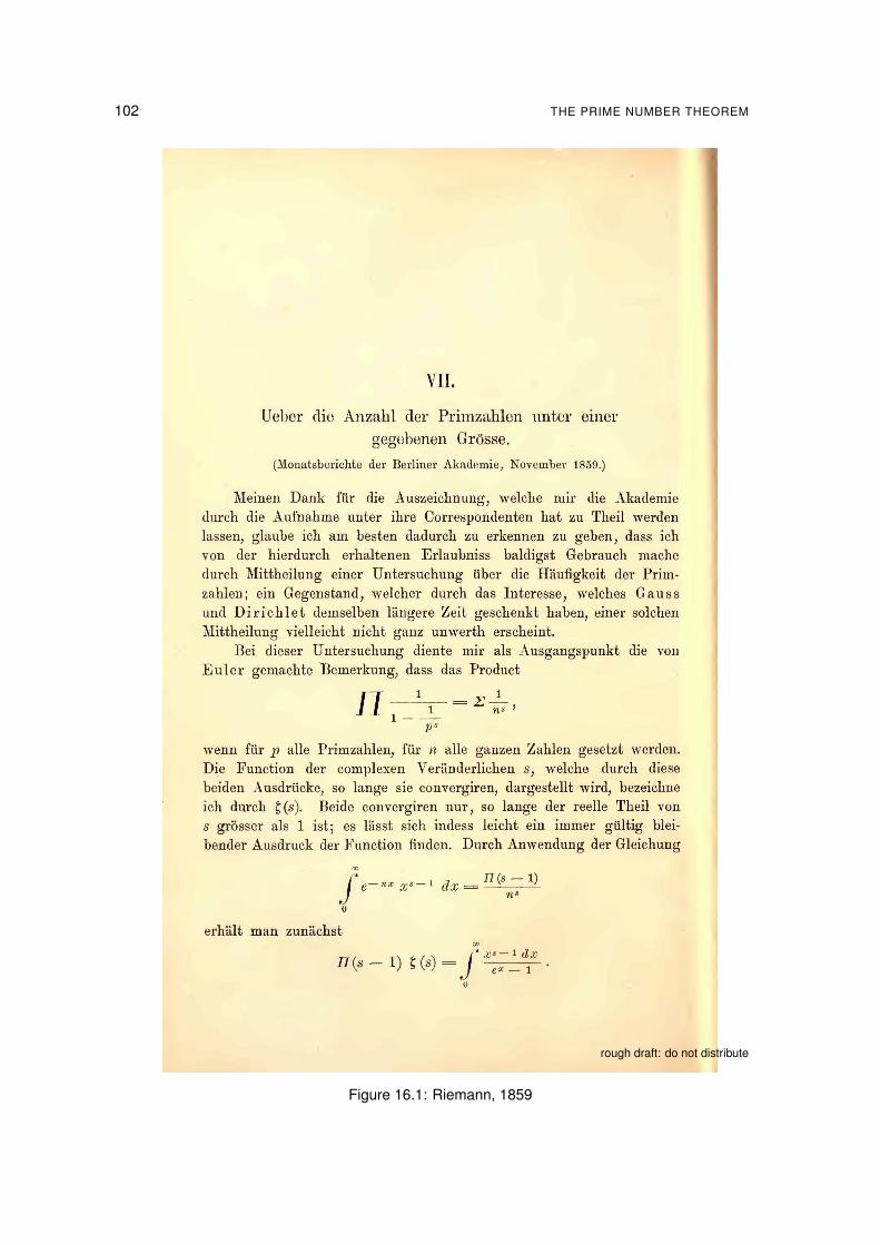
102 THE PRIME NUMBER THEOREM

VII.

Ueber die Anzahl der Primzahlen unter e111er gegebenen GrÖsse.

(Monatsberichte der Berliner Akademie, November 1859.)

Meinen Dank für die Auszeichnung, welche mir die Akademie durch die Aufnahme unter ihre Correspondenten hat zu Theil werden lassen, glaube ich am besten dadurch zu erkennen zu geben, dass ich von der hierdurch erhaltenen Erlaubniss baldigst Gebrauch mache durch Mittheilung einer Untersuchung über die Häufigkeit der Primzahlen; ein Gegenstand, welcher durch das Interesse, welches Gauss und Di richl et demselben längere Zeit geschenkt haben, einer solchen Mittheilung vielleicht nicht ganz unwerth erscheint.

Bei dieser Untersuchung diente mir als Ausgangspunkt die von Euler gemachte Bemerkung, dass das Product

JI __ 1 __ = E _ 1_ 1 n s ,

- 1 --P"

wenn für p alle Primzahlen, für n alle ganzen Zahlen gesetzt werden. Die Function der complexen Veriinderlichen s, welche durch diese beiden Ausdrücke, so lange sie convergiren, dargestellt wird, bezeichne ich durch ~(s). Beide convergiren nur, so lange der reelle Theil von s grässer als 1 ist; es lässt sich indess leicht ein immer güHig bleibender Ausdruck der Function finden. Durch Anwendung der Gleichung

'"

J' e- nx X S - 1 dx = 17 (s - 1) n'

o

erhält man zunächst Cf>

n (S - 1) ~ (s) = J' .~s- l (l x ex - 1 .

o

Figure 16.1: Riemann, 1859


16.2 THE PRIME NUMBER THEOREM 103

Proof. Recall from (15.8) that

−P′(s) =∑

p prime

log pps= sˆ ∞

1

ϑ(x)xs+1 dx = s

ˆ ∞0

e−s tϑ(et

)dt .

From (9.13) we have that

−ζ ′(s)ζ (s)

=∑

p prime

log pps − 1

=∑

p prime

log pps+

∑p prime

log pps (ps − 1)

.

By Theorem 16.1, ζ (s) , 0 for <(s) ≥ 1 and so it follows that

g(s − 1) := −P′(s)

s−

1s − 1

= −1sζ ′(s)ζ (s)

−1

s − 1︸︷︷︸analytic for <(s)≥1

−1s

∑p prime

log pps (ps − 1)︸︷︷︸

analytic for <(s)>1/2

extends to an analytic function in <(s) ≥ 1, i.e.,

g(z) = −P′(z + 1)

z + 1−

1z=

ˆ ∞0

(ϑ(et

)e−t − 1

)︸︷︷︸f (t)

e−zt dt

extends to an analytic function for<(z) ≥ 0. By Chebyshev’s theorem (see (15.9)), the integrandf is bounded by log 4 − 1. It follows from Theorem 14.8 that g(0) =

´ ∞0 f (t) dt =

´ ∞1

ϑ(x)−xx2 dx

exists.

16.2 THE PRIME NUMBER THEOREM

Theorem 16.4 (Prime number theorem, PNT; Hadamard and de la Vallée Poussin,1 1896). Itholds that

π(x) ∼x

log xas x → ∞.

Proof. In view of Corollary 15.14 it is enough to verify that ϑ(x) ∼ x (cf. Remark 15.8). To thisend recall from Theorem 16.3 that

´ ∞1

ϑ(x)−xx2 dx converges.

Assume, by contraposition, that ϑ(x) / x, then there are λ > 1 and µ < 1 so that ϑ(x) > λxor ϑ(x) < µx for arbitrary large x > 0.

In the first case, as ϑ is nondecreasing,ˆ λx

x

ϑ(t) − tt2 dt ≥

ˆ λx

x

λx − tt2 dt =

ˆ λ

1

λ − tt2 dt > 0,

and in the second ˆ x

µx

ϑ(t) − tt2 dt ≤

ˆ x

µx

µx − tt2 dt =

ˆ 1

µ

µ − tt2 dt < 0.

As x is arbitrary large, it follows that the integral´ ∞

1ϑ(x)−x

x2 dx does not converge. This contradictsTheorem 16.3.

1Charles Jean de la Vallée Poussin, 1866–1962, Belgian



Corollary 16.5. For every ε > 0 there is an n0 ∈ N so that there is a prime p with

n < p < (1 + ε)n n ≥ n0.

Proof. By the prime number theorem,

limx→∞

π((1 + ε)x

)π(x)

= limx→∞

(1+ε)xlog

((1+ε)x

)x

log x

= (1 + ε) limx→∞

log xlog x + log(1 + ε)

= 1 + ε. (16.2)

Therefore, there is n0 so that π((1 + ε)x

)> π(x) for all x > n0 and hence there is p ∈ P between

x and (1 + ε)x.

16.3 CONSEQUENCES OF THE PRIME NUMBER THEOREM

Lemma 16.6. Let(an

)n∈N and

(bn

)n∈N are sequences with limn→∞ an = limn→∞ bn = ∞ and

π(an

)∼ π

(bn

),

then alsoan ∼ bn

as n → ∞.

Proof. We show first that lim supn→∞an

bn≤ 1.

Suppose this were false. Then there is ε > 0 and nk with nk → ∞ such that ank > (1 + ε)bnk .Then

lim supn→∞

π(ank

)π(bnk

) ≥ lim supn→∞

π((1 + ε)bnk

)π(bnk

) = 1 + ε

by (16.2), which is a contradiction to the assertion.By exchanging the roles of an and bn it follows that lim supn→∞ b

an≤ 1 and thus limn→∞

an

bn=

1.

Corollary 16.7. Let pn denote the nth prime (cf. (15.2)), then it holds that

pn ∼ n log n (16.3)

as n → ∞.

Proof. By the prime number theorem

π(n log n) ∼n log n

log(n log n)=

n log nlog n + log log n

=n

1 + log log nlog n

∼ n = π(pn).

The assertion follows from the preceding lemma.

Corollary 16.8 (Erdos2). It holds that

pn+1pn−−−−→n→∞

1.

Proof. Indeed, by (16.3), pn+1pn∼

(n+1) log(n+1)n log n −−−−→

n→∞1.

2Paul Erdos, 1913–1996, Hungarian


16.3 CONSEQUENCES OF THE PRIME NUMBER THEOREM 105

Theorem 16.9 (See Theorem 13.29 above). It holds that∑p≤x

1p∼ log log x.

More generally, ∑p≤x

1p∼ log log x + M + O

(1

log x

),

where M := γ +∑

k=2µ(k)k log ζ (k) = 0.261 497 212 . . . is the Meissel3–Mertens constant.

Remark 16.10. Euler actually writes∑∞

p prime1p = log log∞.

Proof. We have from Theorem 15.13 that π(n) = nlog n + O

(n

log2 n

). Hence

∑p≤x

1p=

x∑n=1

π(n) − π(n − 1)n

=

x∑n=1

π(n)n−

x−1∑n=0

π(n)n + 1

=π(x)

x+

x−1∑n=1

π(n)n(n + 1)

=π(x)

x+

x−1∑n=1

π(n)n2 −

x−1∑n=1

π(n)n2(n + 1)

=

x−1∑n=1

π(n)n2 + O(1)

=

x−1∑n=1

(1

n log n+ O

(1

n log2 n

))+ O(1)

= log log x + O(1),

where we have used that 1x log x = (log log x)′ and 1

x log2 x=

(− 1

log x

) ′.

Remark 16.11. Mertens actually proved the statement without employing the prime numbertheorem.

3Ernst Meissel, 1826–1895, German astronomer




17Riemann’s approach by employing the zeta function

This section repeats Riemann’s path. Here we proceed formally and care about convergencelater.

17.1 MERTENS’ FUNCTION

Assume that f (ρ) = 0, then the series expansion is

f (s) = 0 + f ′(ρ)(s − ρ) +(s − ρ)2

2f ′′(ρ) + O(s − ρ)3,

or, assuming that ρ is a simple zero (i.e., f ′(ρ) , 0),

1f (s)

=1

f ′(ρ)(s − ρ)−

f ′′(ρ)2 f ′(ρ)2 + O(s − ρ)1,

the residue at s = ρ is 1f ′(ρ) .

Recall from (9.9) that 1ζ (s) =

∑n=1

µ(n)ns and from (13.9) that M (x) =

∑n≤x µ(n). Assuming that

all all zeros are simple it follows from Perron’s formula (12.4) that

M∗(x) =∑∗

n≤x

µ(n) =ˆ c+i∞

c−i∞

1ζ (s)

xs

sds =

1ζ (0)

+∑

ρ : ζ (ρ)=0

xρ

ρ · ζ ′(ρ)+

∑n=1

x−2n

−2n · ζ ′(−2n),

where the sum is along all zeros ρ of the ζ-function on the critical strip.

17.2 CHEBYSHEV SUMMATORY FUNCTION ψ

Theorem 17.1 (Riemann-von Mangoldt explicit formula). For any x > 1 it holds that

ψ∗(x) = x −∑

ρ : ζ (ρ)=0

xρ

ρ− log 2π −

12

log(1 − x−2

). (17.1)

Proof. The summatory function is∑∗

n≤x ψ(x) =∑∗

n≤x Λ(n), cf. (15.6). Recall from (9.12) theDirichlet series ζ ′(s)

ζ (s) = −∑

n=1Λ(n)ns and the residue is Res

(ζ ′(s)ζ (s) , s = ρ

)= 1. With Perron’s formula

thus

ψ∗(x) =∑∗

n≤x

Λ(n)

=1

2πi

ˆ c+i∞

c−i∞

(−ζ ′(s)ζ (s)

)xs

sds

= x −ζ ′(0)ζ (0)

−∑n=1

x−2n

−2n−

∑ρ

xρ

ρ

= x −∑ρ

xρ

ρ− log 2π −

12

log(1 − x−2

).

107

108 RIEMANN’S APPROACH BY EMPLOYING THE ZETA FUNCTION

17.3 RIEMANN PRIME COUNTING FUNCTION

Theorem 17.2. For x > 1it holds that

J∗(x) = li(x) −∑

ρ : ζ (ρ)=0li(xρ) − log 2 +

ˆ ∞2

dtt(t2 − 1) log t

.

Remark 17.3. We note that li(xρ) = Ei(ρ log x)

Proof. Recall that we have

J∗(x) =∑∗

pk ≤x

1k=

∑∗

n≤x

Λ(n)log n

=

ˆ x

0

1log t

dψ∗(t)

and thus, with (17.1),

J∗(x) =ˆ x

0

ψ∗′(t)log t

dt

=

ˆ x

0

1 −∑ρ tρ−1 − 1

t3−t

log tdt

= li(x) −∑ρ

li(xρ) − log 2 +ˆ ∞x

dtt(t2 − 1) log t

. (17.2)

Indeed, ddx li(xρ) = ρxρ−1

log(xρ ) =xρ−1

log x .

17.4 PRIME COUNTING FUNCTION π

Theorem 17.4. For x > 1 it holds that

π(x) = R(x) −∑ρ

R(xρ) −1

log x+

1π

arctanπ

log x

= R(x) −1

log x+

1π

arctanπ

log x−

∑n=1

µ(n)n

∑j=1

Ei(ρ j log x)

where

R(x) :=∑n=1

µ(n)n

li(x1/n) = 1 +

∑k=1

logk xk! k ζ (k + 1)

(17.3)

is Riemann’s R-function (cf. (15.3)). The latter series is know as Gram1 series.

Recall that we have π∗(x) =∑

k=1µ(k)k J

(x1/k ) and with (17.2) thus

π∗(x) =∑∗

k≤x

1 = R(x) −∑ρ

R(xρ) −1

log x+

1π

arctanπ

log x,

1Jørgen Pedersen Gram, Danish actuary and mathematician


17.4 PRIME COUNTING FUNCTION π 109

Proof of (17.3), Riemann’s R-function. With (14.2) and (9.10) it holds that

R(x) =∑n=1

µ(n)n

li(x1/n) =∑

n=1

µ(n)n

Ei(log x

n

)

=∑n=1

µ(n)n

*,γ − log n + log log x +

∑k=1

logk xk k! nk

+-

=(γ + log log x

) ∑n=1

µ(n)n−

∑n=1

µ(n) log nn

+∑k=1

logk xk k!

∑n=1

µ(n)nk+1 ,

thus the result (cf. also Exercise 10.2).For the rest see Riesel and Gohl [16].


110 RIEMANN’S APPROACH BY EMPLOYING THE ZETA FUNCTION


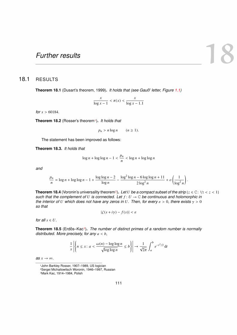
18Further results

18.1 RESULTS

Theorem 18.1 (Dusart’s theorem, 1999). It holds that (see Gauß’ letter, Figure 1.1)

xlog x − 1

< π(x) <x

log x − 1.1

for x > 60184.

Theorem 18.2 (Rosser’s theorem1). It holds that

pn > n log n (n ≥ 1).

The statement has been improved as follows:


log n + log log n − 1 <pnn< log n + log log n

and

pnn= log n + log log n − 1 +

log log n − 2log n

−log2 log n − 6 log log n + 11

2 log2 n+ o

(1

log2 n

).

Theorem 18.4 (Voronin’s universality theorem2). Let U be a compact subset of the strip z ∈ C : 1/2 < z < 1such that the complement of U is connected. Let f : U → C be continuous and holomorphic inthe interior of U which does not have any zeros in U. Then, for every ε > 0, there exists γ > 0so that

|ζ (s + iγ) − f (s) | < ε

for all s ∈ U.

Theorem 18.5 (Erdos–Kac3). The number of distinct primes of a random number is normallydistributed. More precisely, for any a < b,

1x

n ≤ x : a <ω(n) − log log n√

log log n≤ b

→

1√

2π

ˆ b

a

e−t2/2 dt

as x → ∞.

1John Barkley Rosser, 1907–1989, US logician2Sergei Michailowitsch Woronin, 1946–1997, Russian3Mark Kac, 1914–1984, Polish

111

112 FURTHER RESULTS

Billingsley’s proof. Let Xp be independent Bernoulli variables with P(Xp = 1) = 1p . Set Sy :=∑

p≤y Xp, then µy := E Sy =∑

p≤y1p = log log y + O(1) and σ2

y := var Sy =∑

p≤y1p −

1p2 =

log log y + O(1) by Theorem 16.9. The central limit theorem implies Sy−µyσy

→ N (0, 1) as y → ∞.

Fix y and let 1p (n) := [p | n] =

1 if p | n0 else

(the Iverson bracket) so that ωy (n) :=∑

p |n, p≤y 1 =∑p≤y 1p (n). We compare the moments of ωy (n) with those of Sy, i.e.,

1x

∑n≤x

(ωy (n) − µy

)k− E

(Sy − µy

)k=

k∑j=1

(kj

) (−µy

)k−y· *

,

1x

∑n≤x

ωy (n) j − E S jy

+-.

The last term is∑p1,...,p j ≤y

*,

1x

∑n≤x

1p1 (n) · · ·1p j (n) − E Xp1 · · · Xp j+-=

∑p1,...,p j ≤y

L:=lcm(p1,...,p j

(1x

⌊ xL

−1L

)

π(y) j

x.

This error bound implies that 1x

∑n≤x

(ωy (n)−µy

σy

)k∼ E

(Sy−µyσy

)k∼ E Zk as y → ∞, where Z ∼

N (0, 1). If we choose y := x1/log log log x , then ω(n) − ωy (n) ≤ log log log x and thus the result.

18.2 OPEN PROBLEMS

Conjecture 18.6 (Goldbach’s4 conjecture). Every even integer greater than 2 can be expressedas the sum of two primes.

Conjecture 18.7 (Twin prime conjecture). There exist infinity many twin primes (cf. Defini-tion 2.19).

Problem 18.8 (Landau’s 4th problem). Are there infinitely many primes of the form n2 + 1?

4Christian Goldbach, 1690–1764, German mathematician


Bibliography

[1] M. Abramowitz and I. A. Stegun. Handbook of Mathematical Functions with Formulas,Graphs, and Mathematical Tables. Dover, New York, ninth Dover printing, tenth GPO print-ing edition, 1964. ISBN 0-486-61272-4. URL http://people.math.sfu.ca/~cbm/aands/frameindex.htm. 40

[2] T. M. Apostol. Introduction to Analytic Number Theory. Springer New York, 1976.doi:10.1007/978-1-4757-5579-4. 7

[3] H. Bateman. Tables of Integral Transforms. McGraw-Hill Book Company, Inc., New York-Toronto-London, 1954. 67

[4] P. Borwein, S. Choi, B. Rooney, and A. Weirathmueller, editors. The Riemann Hypothesis.Springer New York, 2008. doi:10.1007/978-0-387-72126-2. 7

[5] H. Davenport. Multiplicative Number Theory. Springer New York, 1980. doi:10.1007/978-1-4757-5927-3. 7

[6] D. Duverney. Number Theory. WORLD SCIENTIFIC, 2010. doi:10.1142/7762. 25

[7] H. M. Edwards. Riemann’s Zeta Function. Academic Press, New York and London, 1974.URL https://books.google.at/books?id=ruVmGFPwN. 7, 78

[8] O. Forster. Analytic number theory. Lecture notes, TU München, 2001. URL http://www.mathematik.uni-muenchen.de/~forster/v/ann/annth_all.pdf. 7

[9] G. H. Hardy and M. Riesz. The General Theory Of Dirichlets Series. 1915. URL https://archive.org/details/generaltheoryofd029816mbp/. 65

[10] G. H. Hardy and E. M. Wright. An introduction to the theory of numbers, 6th edition. 51(3):283–283, 2010. doi:10.1080/00107510903184414. 7

[11] H. Hasse. Ein Summierungsverfahren für die Riemannsche ζ-Reihe. MathematischeZeitschrift, 32(1):458–464, 1930. doi:10.1007/BF01194645. German. 79

[12] H. Ivaniec and E. Kowalski. Analytic Number Theory, volume 53 of Colloquium Publications.American Mathematical Society, Providence, Rhode Island, 2004. ISBN 0-8218-3633-1.doi:10.1090/coll/053. 7

[13] S. Khrushchev. Orthogonal Polynomials and Continued Fractions. Cambridge UniversityPress, 2011. ISBN 0521854199. URL https://www.maths.ed.ac.uk/~v1ranick/papers/khrushchev.pdf. 25

[14] D. J. Newman. Simple analytic proof of the prime number theorem. The American Mathe-matical Monthly, 87(9):693–696, 1980. doi:10.2307/2321853. 7, 91, 101

[15] B. Riemann. Werke. Leipzig: Druck und Verlag von B. G. Teubner, 1876. German. 75

[16] H. Riesel and G. Gohl. Some calculations related to Riemann’s prime number formula.Mathematics of Computation, 24(112):969–983, 1970. doi:10.2307/2004630. 109

113

http://people.math.sfu.ca/~cbm/aands/frameindex.htm

http://people.math.sfu.ca/~cbm/aands/frameindex.htm

http://dx.doi.org/10.1007/978-1-4757-5579-4

http://dx.doi.org/10.1007/978-0-387-72126-2

http://dx.doi.org/10.1007/978-1-4757-5927-3

http://dx.doi.org/10.1007/978-1-4757-5927-3

http://dx.doi.org/10.1142/7762

https://books.google.at/books?id=ruVmGFPwN

http://www.mathematik.uni-muenchen.de/~forster/v/ann/annth_all.pdf

http://www.mathematik.uni-muenchen.de/~forster/v/ann/annth_all.pdf

https://archive.org/details/generaltheoryofd029816mbp/

https://archive.org/details/generaltheoryofd029816mbp/

http://dx.doi.org/10.1080/00107510903184414

http://dx.doi.org/10.1007/BF01194645

http://dx.doi.org/10.1090/coll/053

https://www.maths.ed.ac.uk/~v1ranick/papers/khrushchev.pdf

https://www.maths.ed.ac.uk/~v1ranick/papers/khrushchev.pdf

http://dx.doi.org/10.2307/2321853

http://dx.doi.org/10.2307/2004630

114 BIBLIOGRAPHY

Figure 18.1: Homer cubed

[17] Sander. Analytische Zahlentheorie. Lecture notes (in German), Universität Hannover, 2001.URL http://www.blu7.com/Skripte/Analytische_Zahlentheorie_SS01_Skript.pdf. 7

[18] E. C. Titchmarsh. The Zeta-Function of Riemann. 1930. 7

[19] E. C. Titchmarsh. The Theory of the Riemann Zeta function. Oxford University Press,Providence, Rhode Island, second edition, 1986. ISBN 0-19-853369-1. 7, 55

[20] H. S. Wall. Analytic theory of continued fractions. Chelsea Publ., 1948. 25

[21] D. Zagier. Die ersten 50 Millionen Primzahlen. In Lebendige Zahlen, pages 39–73.Birkhäuser Basel, 1981. doi:10.1007/978-3-0348-5407-8. German. 7

[22] D. Zagier. Newman’s short proof of the prime number theorem. The American Mathemati-cal Monthly, 104(8), 1997. doi:10.1080/00029890.1997.11990704. 7, 91, 101


https://www.youtube.com/watch?v=7824c5YAsEA

http://www.blu7.com/Skripte/Analytische_Zahlentheorie_SS01_Skript.pdf

http://dx.doi.org/10.1007/978-3-0348-5407-8

http://dx.doi.org/10.1080/00029890.1997.11990704

Index

BBernoulli

number, 31polynomial, 31

Bézout identity, 10

Ccomposite, 10coprime, 10

DDirichlet

inverse, 59product, 59series, 65

EEuclid’s lemma, 11Euler–Mascheroni constant, 36exponential integral, 89

FFermat

liar, 23pseudoprime, 23

functionadditive, 51arithmetic, 51arithmetic function

divisor, σk , 52Liouville, λ, 51Möbius, µ, 53number-of-divisors, σ0, 52prime omega, big omega, Ω, 51prime omega, ω, 51sum-of-divisors, σ, 52totient, ϕ, 19von Mangoldt, Λ, 55

Chebyshev, ϑ, ψ, 95multiplicative, 51totally multiplicative, 51

fundamental theorem of arithmetic, 12

GGamma function, 35

gcd, 10

HHeaviside step function, 67

Lleast common multiple, lcm, 9logarithmic integral, 90

MMöbius inversion, 60multiple, 10

Nnumber

Carmichael, 23

Pprime, 10

cousin, 13sexy, 13twin, 13

prime gap, 13prime number theorem, 103prime-counting function, π, 93primes

Fermat, 14Mersenne, 14

primorial, 95

RRiemann hypothesis, 87Riemann-Siegel, 86

SStieltes constants, 81Stirling formula, 40summation

Abel, 47Borel, 48by parts, 45Cesàro, 44Euler, 44Euler–Maclaurin, 39Lambert, 46

115

116 INDEX

Poisson, 47

WWallis’ product, 37

Zzeros

non-obvious, 87trivial, 80

zeta function, 52prime P, 56


Date post:	28-Oct-2019
Category:	Documents
Upload:	others
View:	29 times
Download:	2 times

Introduction to Analytic Number Theory - tu-chemnitz.de · In number theory, the fundamental...

Documents