Introduction to Automatic Speech Recognition Prof. Dr.-Ing. Hermann Ney, Dr. Ralf Schl¨ uter Lehrstuhl f¨ ur Informatik 6 Human Language Technology and Pattern Recognition Computer Science Department, RWTH Aachen University D-52056 Aachen, Germany October 20, 2009 Ney/Schl¨ uter: Introduction to Automatic Speech Recognition 1 October 20, 2009
Transcript
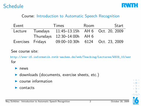
Introduction to Automatic Speech Recognition
Prof. Dr.-Ing. Hermann Ney, Dr. Ralf Schluter
Lehrstuhl fur Informatik 6Human Language Technology and Pattern Recognition
Ney/Schluter: Introduction to Automatic Speech Recognition 3 October 20, 2009
Outline0. Lehrstuhl fur Informatik 60.1 Research Topics0.2 Projects0.3 Courses0.4 Textbooks
1. Introduction to Speech Recognition
2. Digital Signal Processing
3. Spectral Analysis
4. Time Alignment and Isolated Word Recognition
5. Statistical Interpretation and Models
6. Connected Word Recognition
7. Large Vocabulary Speech Recognition
Ney/Schluter: Introduction to Automatic Speech Recognition 4 October 20, 2009
Lehrstuhl fur Informatik 6: Research TopicsResearch Topics
Method: Stochastic Modelling
I Modelling dependencies and vague knowledge(contrast: rule-based approach)
I Decision making, in particular in context
I Automatic learning from data/examples
Applications:Human Language Technology and Pattern Recognition
Ney/Schluter: Introduction to Automatic Speech Recognition 5 October 20, 2009
Applications: Examples
I Speech recognition
I small vocabularyI large vocabulary
I Machine translation
I Natural language processing
I text/document classificationI information retrievalI parsing and syntactic analysis
I Language understanding and dialog systems
I Image recognition
I object recognitionI handwriting recognition
Ney/Schluter: Introduction to Automatic Speech Recognition 6 October 20, 2009
Applications: Examples
I Diagnosis and expert systems
I Other applications:
I speaker verification and identificationI fingerprint verification and identificationI DNA sequence identificationI gesture recognitionI lip readingI geological analysisI high-energy physics: bubble chamber tracksI ...
Ney/Schluter: Introduction to Automatic Speech Recognition 7 October 20, 2009
Outline0. Lehrstuhl fur Informatik 60.1 Research Topics0.2 Projects0.3 Courses0.4 Textbooks
1. Introduction to Speech Recognition
2. Digital Signal Processing
3. Spectral Analysis
4. Time Alignment and Isolated Word Recognition
5. Statistical Interpretation and Models
6. Connected Word Recognition
7. Large Vocabulary Speech Recognition
Ney/Schluter: Introduction to Automatic Speech Recognition 8 October 20, 2009
Lehrstuhl fur Informatik 6 (i6): Projects
I ARISE (EU):Automatic Railway Information Systems across Europe– Speech Recognition and Language Modelling
I EuTrans II (EU): Translation of Spoken Language– Speech Recognition and Translation
I Institut fur deutsche Sprache (IdS):– Language Modelling for Newspapers
I Audio Document Retrieval (NRW):– Speech Recognition and Information Retrieval
I Verbmobil II (BMBF): Speech Recognition and Translation forAppointment Scheduling and Traveling Information– Speech Recognition– Speech Translation– Prototype Modules
Ney/Schluter: Introduction to Automatic Speech Recognition 9 October 20, 2009
Projects i6
I Image Object Recognition (RWTH):– OCR (optical character recognition)– Medical Images
I Advisor (EU):– Speech Recognition for German Broadcast News
I EGYPT follow-up (NSF):– Basic Algorithms for Statistical Machine Translation
I Audio Document Retrieval (NRW ?):– German Broadcast News: Recognition and Information Retrieval
I Bilateral Projects with Companies (including start-ups)
I German DFG:– Improved Acoustic Modelling using Structured Models– Statistical Methods for Written Language Translation– Statistical Modeling for Image Object Recognition
Ney/Schluter: Introduction to Automatic Speech Recognition 10 October 20, 2009
Projects i6I Coretex (EU):
– Improving Core Technology for Speech Recognition– Applications: Broadcast News in Several Languages
I LC-Star (EU):– Lexical and Corpora Resources for Recognition, Translationand Synthesis– Prototype system for machine translation of spokensentences
I TC-Star (EU):– Technology and Corpora for Speech to Speech Translation– Applications: Broadcast News and Speeches/Lectures
I Transtype-2 (EU):– Machine translation of written text– Application: interactive machine-aided translation
I PF-Star (EU):– Machine translation of spoken dialogues– Application: tourism and travelling
Ney/Schluter: Introduction to Automatic Speech Recognition 11 October 20, 2009
Projects i6
I JUMAS (EU):– Judicial MAnagement by digital libraries Semantics– Application: audio and video search of court proceedings
I LUNA (EU):– spoken Language UNderstanding in multilinguAl
communication systems
– Application: real-time understanding of spontaneous speechin advanced telecom services
I GALE (US-DARPA):– Global Autonomous Language Exploitation– Application: Information Processing in Multiple Languages
I QUAERO [lat.: to search] (OSEO/France)– multimedia and multilingual indexing– Application: extract information from written texts,
speech and music audio, images, and video
Ney/Schluter: Introduction to Automatic Speech Recognition 12 October 20, 2009
Outline0. Lehrstuhl fur Informatik 60.1 Research Topics0.2 Projects0.3 Courses0.4 Textbooks
1. Introduction to Speech Recognition
2. Digital Signal Processing
3. Spectral Analysis
4. Time Alignment and Isolated Word Recognition
5. Statistical Interpretation and Models
6. Connected Word Recognition
7. Large Vocabulary Speech Recognition
Ney/Schluter: Introduction to Automatic Speech Recognition 13 October 20, 2009
Courses
I Introductory lectures (L3/4) with exercises (E2) for Bachelor,Master, and Diploma students:– ASR: (Introduction to) Automatic Speech Recognition– PRN: (Introduction to) Pattern Recognition and Neural Networks– NLP: (Introduction to) Natural Language Processing
I Advanced lectures (L3) with exercises (E1/2) for Master andDoctoral students:– advASR: Advanced Automatic Speech Recognition– advPRN: Advanced Pattern Recognition– advNLP: Advanced Natural Language Processing
I Further Lectures (L2) with exercises (E1):– MIP: Medical Image Processing
(’Ringvorlesung’, each WS)
Ney/Schluter: Introduction to Automatic Speech Recognition 14 October 20, 2009
Courses (ctd.)
I Seminars:– Bachelor Degree (SS, Block)– Diplom Degree (SS, Block)– Doctor Degree (WS+SS)
I Laboratory Courses (WS, Block)
I Study Groups (WS+SS: speech, language, image)
New course cycles:year term lectures
08/09 WS PRNN (L4/3,E2) ASR (L4/3,E2)SS NLP (L4/3,E2) –
09/10 WS PRNN (L4/3,E2) ASR (L4/3,E2)SS NLP (L4/3,E2) advASR (L3,E1)
Ney/Schluter: Introduction to Automatic Speech Recognition 15 October 20, 2009
Exams i6: Diplom Degree
I area of specialization (Vertiefungsgebiet) i6 with the topics:
– Automatic Speech Recognition (ASR)– Pattern Recognition and Neural Networks (PRNN)– Natural Language Processing (NLP)– ...select 12 hours (SWS) out of i6 lectures
Ney/Schluter: Introduction to Automatic Speech Recognition 16 October 20, 2009
Exams i6: Diplom Degree (ctd.)
I practical computer science (Prakt. Informatik) (3 areas):recommendation: 12 hours (SWS) out of
two L4 from: ASR, PRNN, NLPone L4 from i6-external lectures:
I data basesI artificial intelligenceI ... additional alternatives: on demand
Ney/Schluter: Introduction to Automatic Speech Recognition 17 October 20, 2009
Examinations i6
I Bachelor Informatik:credit system: oral exam after each course/at end of lecture period
I Master in Media Informatics or Software Systems Engineering:credit system: oral exam after each course/at end of lecture period
I Technische Informatik (Diplom):oral exam at the end of the lecture period (exception)
I Magister in Technik-Kommunikation:more or less similar to Diplom degree
I ERASMUS students of Computer Science:oral exam/colloquium for graded certificate at end of lecture period
Note: consult Prof. Ney before December 2009 for exam dates,and before registering for the exam with the ZPA. The ZPAregistration period via CAMPUS Office is Dec. 1-18, 2009; theexam registration in person at ZPA is expected to be Dec. 2/3,2009.
Ney/Schluter: Introduction to Automatic Speech Recognition 18 October 20, 2009
Outline0. Lehrstuhl fur Informatik 60.1 Research Topics0.2 Projects0.3 Courses0.4 Textbooks
1. Introduction to Speech Recognition
2. Digital Signal Processing
3. Spectral Analysis
4. Time Alignment and Isolated Word Recognition
5. Statistical Interpretation and Models
6. Connected Word Recognition
7. Large Vocabulary Speech Recognition
Ney/Schluter: Introduction to Automatic Speech Recognition 19 October 20, 2009
Textbooks: Topics i6Textbooks on Speech Recognition:
I emphasis on signal processing and small-vocabularyrecognition:L. Rabiner, B. H. Juang: Fundamentals of SpeechRecognition.Prentice Hall, Englewood Cliffs, NJ, 1993.
I emphasis on large vocabulary and language modelling:F. Jelinek: Statistical Methods for Speech Recognition.MIT Press, Cambridge, 1997.
I introduction to both speech and language:D. Jurafsky, J. H. Martin: Speech and Language Processing.Prentice Hall, Englewood Cliffs, NJ, 2000.
I advanced topics:R. De Mori: Spoken Dialogues with Computers.Academic Press, London, 1998
Ney/Schluter: Introduction to Automatic Speech Recognition 20 October 20, 2009
Textbooks: Topics i6Textbooks on Signal Processing:
I A. V. Oppenheim, R. W. Schafer: Discrete Time SignalProcessing, Prentice Hall, Englewood Cliffs, NJ, 1989.
I A. Papoulis: Signal Analysis, McGraw-Hill, New York, NY, 1977.I A. Papoulis: The Fourier Integral and its Applications,
McGraw-Hill Classic Textbook Reissue Series, McGraw-Hill,New York, NY, 1987.
I W. K. Pratt: Digital Image Processing, Wiley & Sons Inc,New York, NY, 1991.
Further reading on Signal Processing:I T. K. Moon, W. C. Stirling: Mathematical Methods and Algorithms
for Signal Processing. Prentice Hall, Upper Saddle River, NJ, 2000.I J. R. Deller, J. G. Proakis, J. H. L. Hansen: Discrete-Time
Processing of Speech Signals, Macmillan Publishing Company,New York, NY, 1993.
I L. Berg: Lineare Gleichungssysteme mit Bandstruktur, VEBDeutscher Verlag der Wissenschaften, Berlin, 1986.
Ney/Schluter: Introduction to Automatic Speech Recognition 21 October 20, 2009
Textbooks: Topics i6
Textbooks on Natural Language Processing(statistical/corpus-based):
I introduction to both speech and language:D. Jurafsky, J. H. Martin: Speech and Language Processing.Prentice Hall, Englewood Cliffs, NJ, 2000.
I emphasis on statistical methods for written language:C. D. Manning, H. Schutze: Foundations of Statistical NaturalLanguage Processing. MIT Press, Cambridge, MA, 1999.
I related field: artificial intelligence:S. Russel, P. Norvig: Artificial Intelligence. Prentice Hall,Englewood Cliffs, NJ, 1995 (in particular Chapters 22-25).
Ney/Schluter: Introduction to Automatic Speech Recognition 22 October 20, 2009
Textbooks: Topics i6Textbooks on Statistical Learning (Pattern Recognition, NeuralNetworks, Data Mining, ...):
I best introduction (including modern concepts):R. O. Duda, P. E. Hart, D. G. Stork: Pattern Classification.2nd ed., J. Wiley & Sons, New York, NY, 2001.
I emphasis on statistical concepts:B. D. Ripley: Pattern Recognition and Neural Networks.Cambridge University Press, Cambridge, England, 1996.
I emphasis on modern statistical concepts:T. Hastie, R. Tibshirani, J. Friedman: The Elements ofStatistical Learning: Data Mining, Inference and Predictions.Springer, New York, 2001.
I emphasis on theory and principles:L. Devroye, J. Gyorfi, G. Lugosi: A Probabilistic Theory ofPattern Recognition. Springer, New York, 1996.
Ney/Schluter: Introduction to Automatic Speech Recognition 23 October 20, 2009
Textbooks: Topics i6
Textbooks on mathematical methods (vector spaces and matrices,statistics, optimization methods, ...):
I best overall summary:T. K. Moon, W. C. Stirling: Mathematical Methods andAlgorithms for Signal Processing. Prentice Hall, Upper SaddleRiver, NJ, 2000.
I introduction to modern statistics:G. Casella, R. L. Berger: Statistical Inference. Wadsworth &Brooks/Cole, Pacific Grove, CA, 1990.
I good overview of numerical algorithms and implementations:W. H. Press, S. A. Teukolsky, W. T. Vetterling,B. P. Flannery: Numerical Recipes in C. CambridgeUniv. Press, Cambridge, 2nd ed., 1992.
Ney/Schluter: Introduction to Automatic Speech Recognition 24 October 20, 2009
Outline0. Lehrstuhl fur Informatik 6
1. Introduction to Speech Recognition1.1 Task Definition & History1.2 History1.3 Why is Speech Recognition Hard?1.4 Stochastic Approach1.5 Evaluation1.6 Examples
2. Digital Signal Processing
3. Spectral Analysis
4. Time Alignment and Isolated Word Recognition
5. Statistical Interpretation and Models
6. Connected Word Recognition
7. Large Vocabulary Speech Recognition
Ney/Schluter: Introduction to Automatic Speech Recognition 25 October 20, 2009
What is speech recognition?
Speech recognition means:
convert the acoustic signal (sound) into a sequence ofwritten words (text)
Related tasks:
I Speech understanding: generating a semantic representation
I Speaker recognition: identifying the person who spoke
I Speech detection: separating speech from non-speech
I Speech enhancement: improve the intelligibility of a signal
I Speech compression: encode speech signal for transmissionor storage with a small amount of bits
Ney/Schluter: Introduction to Automatic Speech Recognition 26 October 20, 2009
Terminology: Speech Recognition vs. Understanding
I Speech recognition (Spracherkennung)typical application: dictation, i.e. speech to text;understanding is secondary.
I Speech (or language) understanding (Sprachverstehen)recognition AND ‘logical’ understanding:
I easy application:Recognize 1 of K voice commands andcarry them out (e.g. name dialing).
I difficult application:Spoken dialogue system with natural language input(e.g. travel information)
Ney/Schluter: Introduction to Automatic Speech Recognition 27 October 20, 2009
Outline0. Lehrstuhl fur Informatik 6
1. Introduction to Speech Recognition1.1 Task Definition & History1.2 History1.3 Why is Speech Recognition Hard?1.4 Stochastic Approach1.5 Evaluation1.6 Examples
2. Digital Signal Processing
3. Spectral Analysis
4. Time Alignment and Isolated Word Recognition
5. Statistical Interpretation and Models
6. Connected Word Recognition
7. Large Vocabulary Speech Recognition
Ney/Schluter: Introduction to Automatic Speech Recognition 28 October 20, 2009
Historical DevelopmentsHistory of speech and language technology:
Ney/Schluter: Introduction to Automatic Speech Recognition 35 October 20, 2009
Outline0. Lehrstuhl fur Informatik 6
1. Introduction to Speech Recognition1.1 Task Definition & History1.2 History1.3 Why is Speech Recognition Hard?1.4 Stochastic Approach1.5 Evaluation1.6 Examples
2. Digital Signal Processing
3. Spectral Analysis
4. Time Alignment and Isolated Word Recognition
5. Statistical Interpretation and Models
6. Connected Word Recognition
7. Large Vocabulary Speech Recognition
Ney/Schluter: Introduction to Automatic Speech Recognition 36 October 20, 2009
Stochastic Modelling for Speech RecognitionKey Ideas:
I put all ambiguities in probability distributions(stochastic knowledge sources)
I stochastic modelling in speech recognition:I phoneme (or word) modelsI pronunciation lexiconI language model
I training: use data to train the free parameters of the models
I leave all the interdependencies and ambiguities to a search process,e.g. 16 values/10 msec = 32 000 values/20 sec:
I optimal interaction between all knowledge sourcesI (virtually) no local (=intermediate) decisionsI no distinction between statistical and syntactic pattern recognition→ holistic approach to decision making
contrast: rule-based system (a la Prolog) withhard decisions at intermediate levels
Ney/Schluter: Introduction to Automatic Speech Recognition 37 October 20, 2009
Knowledge Sources and Interactions in Speech RecognitionSPEECH SIGNAL
ACOUSTIC ANALYSIS
RECOGNIZED SENTENCE
SENTENCE
KNOWLEDGE SOURCESSEARCH: INTERACTION OF
KNOWLEDGE SOURCES
WORD
PHONEME
LANGUAGE MODEL
PRONUNCIATION LEXICON
PHONEMEMODELS
SEGMENTATION ANDCLASSIFICATION
SYNTACTIC ANDSEMANTIC ANALYSIS
WORD BOUNDARY DETECTIONAND LEXICAL ACCESS
HYPOTHESES
HYPOTHESES
HYPOTHESES
Ney/Schluter: Introduction to Automatic Speech Recognition 38 October 20, 2009
Outline0. Lehrstuhl fur Informatik 6
1. Introduction to Speech Recognition1.1 Task Definition & History1.2 History1.3 Why is Speech Recognition Hard?1.4 Stochastic Approach1.5 Evaluation1.6 Examples
2. Digital Signal Processing
3. Spectral Analysis
4. Time Alignment and Isolated Word Recognition
5. Statistical Interpretation and Models
6. Connected Word Recognition
7. Large Vocabulary Speech Recognition
Ney/Schluter: Introduction to Automatic Speech Recognition 39 October 20, 2009
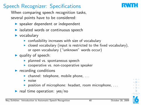
Speech Recognizer: SpecificationsWhen comparing speech recognition tasks,several points have to be considered:
I speaker dependent or independent
I isolated words or continuous speechI vocabulary
I confusibility increases with size of vocabularyI closed vocabulary (input is restricted to the fixed vocabulary),
or open vocabulary (“unknown” words occur)
I quality of speech:I planned vs. spontaneous speechI cooperative vs. non-cooperative speaker
I recording conditionsI channel: telephone, mobile phone, . . .I noiseI position of microphone: headset, room microphone, . . .
I real time operation: yes/no
Ney/Schluter: Introduction to Automatic Speech Recognition 40 October 20, 2009
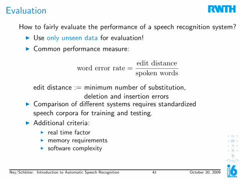
Evaluation
How to fairly evaluate the performance of a speech recognition system?
I Use only unseen data for evaluation!
I Common performance measure:
word error rate =edit distancespoken words
edit distance := minimum number of substitution,deletion and insertion errors
I Comparison of different systems requires standardizedspeech corpora for training and testing.
I Additional criteria:I real time factorI memory requirementsI software complexity
Ney/Schluter: Introduction to Automatic Speech Recognition 41 October 20, 2009
Evaluation
Out of vocabulary (OOV) words:
I words in the testing corpus that arenot included in the recognition vocabulary
I these words can not be recognized correctly
I the OOV rate [%] is a lower bound for the word error rate
I every OOV word leads to at least one recognition error,but the average is about 2 errors per OOV word.
Ney/Schluter: Introduction to Automatic Speech Recognition 42 October 20, 2009
Word Error Rate: ExampleExample from the Verbmobil Corpus
play /example-verbmobil-2.wav
Spoken:
also ich vielleicht ist grade zu der Zeit die CeBit das ware
vielleicht fur uns fachlich auch ganz interessant
Recognized:
also ich vielleicht das grade zu der Zeit die CeBit das ware
vielleicht uns fachlich auch noch ganz interessant
substitution insertion deletion
WER =1 deletion + 1 insertion + 1 substitution
19 spoken words= 15.8%
Ney/Schluter: Introduction to Automatic Speech Recognition 43 October 20, 2009
Outline0. Lehrstuhl fur Informatik 6
1. Introduction to Speech Recognition1.1 Task Definition & History1.2 History1.3 Why is Speech Recognition Hard?1.4 Stochastic Approach1.5 Evaluation1.6 Examples
2. Digital Signal Processing
3. Spectral Analysis
4. Time Alignment and Isolated Word Recognition
5. Statistical Interpretation and Models
6. Connected Word Recognition
7. Large Vocabulary Speech Recognition
Ney/Schluter: Introduction to Automatic Speech Recognition 44 October 20, 2009
play example-sietill-1.wav play example-sietill-2.wav
ARISE (Automatic Railway Information System across Europe)
language: Dutch domain: timetable informationrecording: telephone vocabulary: 1000 words
play example-arise-1.wav
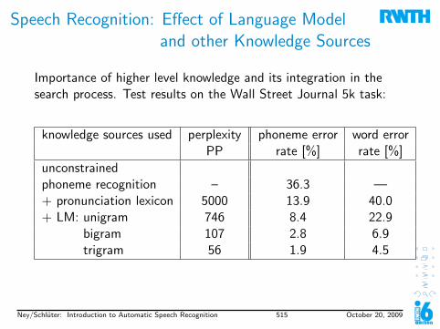
WSJ (Wall Street Journal) 5k
language: American English domain: news paper textrecording: studio quality, vocabulary: 5000 words
read speech
play example-wsj-1.wav play example-wsj-2.wav
Ney/Schluter: Introduction to Automatic Speech Recognition 45 October 20, 2009
Corpora
Verbmobil 2
language: Germandomain: appointments, travel informationrecording: office environment, high quality and telephone recordings
spontaneous speech, various dialectsvocabulary: 10000 words
play example-verbmobil-1.wav play example-verbmobil-3.wav
Ney/Schluter: Introduction to Automatic Speech Recognition 46 October 20, 2009
Corpora
Hub4 (Broadcast News)
language: American Englishdomain: TV and radio broadcasts (CNN Headline News,
NPR All things considered, . . . )recording: various conditions (studio , interviews, reporters, . . . )vocabulary: 65000 words
examples: show demo en.html
Advisor (Broadcast News)
language: Germandomain: TV and radio broadcasts (Report Mainz (SWR), . . . )recording: various conditions (studio , interviews, reporters, . . . )vocabulary: 62000 words
examples: show demo de.html
Ney/Schluter: Introduction to Automatic Speech Recognition 47 October 20, 2009
Corpora
EPPS (European Parliament Plenary Sessions)
language: Spanishdomain: Parliamentary Speechesrecording: parliamentary hall (politicians)vocabulary: 60000 words
examples: show tcstar epps demo.html
Ney/Schluter: Introduction to Automatic Speech Recognition 48 October 20, 2009
Corpora
GALE (Broadcast News)
language: Arabicdomain: TV broadcasts (Al Jazeera News)recording: various conditions (studio , interviews, reporters, . . . )vocabulary: 256000 words (429000 pronunciations)
examples: show demo ar.html
language: Mandarin Chinesedomain: TV broadcasts (CCTV 4 News)recording: various conditions (studio , interviews, reporters, . . . )vocabulary: 60000 words
examples: show demo cn.html
Ney/Schluter: Introduction to Automatic Speech Recognition 49 October 20, 2009
Outline0. Lehrstuhl fur Informatik 6
1. Introduction to Speech Recognition
2. Digital Signal Processing2.1 Motivation2.2 Linear time-invariant Systems2.3 Fourier Transform2.4 δ-Function2.5 Fourier Series2.6 Discrete Time Signal Processing2.7 Sampling (Nyquist) Theorem and Reconstruction2.8 Fourier Transform and z–Transform2.9 System Representation and Examples2.10 Discrete Time Signal Fourier Transform Theorems2.11 Discrete Fourier Transform (DFT)2.12 Fast Fourier Transform (FFT)
3. Spectral Analysis
4. Time Alignment and Isolated Word Recognition
5. Statistical Interpretation and Models
6. Connected Word Recognition
7. Large Vocabulary Speech Recognition
Ney/Schluter: Introduction to Automatic Speech Recognition 50 October 20, 2009
The Speech SignalSpeech Signal Analysis
The acoustic signal is recorded by a microphone and sampled at afrequency of (say) 16 kHz and converted into a sequence of 16-bitnumbers.An example from the Wall Street Journal corpus:play example-1.wav
This acoustic waveform shows very little direct cues about whatmight have been said.Note that not even the word boundaries are obvious.
Ney/Schluter: Introduction to Automatic Speech Recognition 51 October 20, 2009
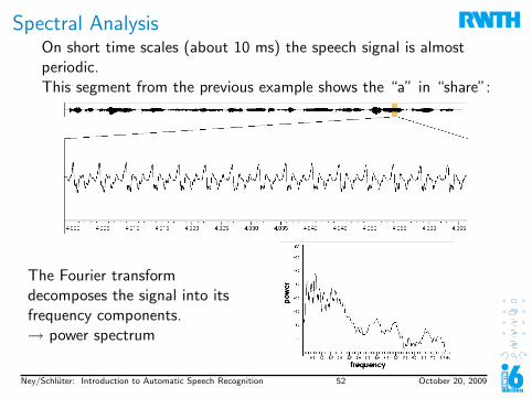
Spectral AnalysisOn short time scales (about 10 ms) the speech signal is almostperiodic.This segment from the previous example shows the “a” in “share”:
The Fourier transformdecomposes the signal into itsfrequency components.→ power spectrum
Ney/Schluter: Introduction to Automatic Speech Recognition 52 October 20, 2009
The Spectrogram
The speech signal is divided into overlapping windowsapproximately 25ms long and 10ms apart. For each so-calledtime-frame the power spectrum is calculated.
This results in a spectrogram which shows the spectral energydistribution for each time-frame:
Ney/Schluter: Introduction to Automatic Speech Recognition 53 October 20, 2009
Ney/Schluter: Introduction to Automatic Speech Recognition 55 October 20, 2009
Outline0. Lehrstuhl fur Informatik 6
1. Introduction to Speech Recognition
2. Digital Signal Processing2.1 Motivation2.2 Linear time-invariant Systems2.3 Fourier Transform2.4 δ-Function2.5 Fourier Series2.6 Discrete Time Signal Processing2.7 Sampling (Nyquist) Theorem and Reconstruction2.8 Fourier Transform and z–Transform2.9 System Representation and Examples2.10 Discrete Time Signal Fourier Transform Theorems2.11 Discrete Fourier Transform (DFT)2.12 Fast Fourier Transform (FFT)
3. Spectral Analysis
4. Time Alignment and Isolated Word Recognition
5. Statistical Interpretation and Models
6. Connected Word Recognition
7. Large Vocabulary Speech Recognition
Ney/Schluter: Introduction to Automatic Speech Recognition 56 October 20, 2009
Linear time-invariant Systems
Examples:
– speech production
– electrical systems
S
h(t)input signal
x(t)output signal
y(t)
symbolic: t → y(t) = S t → x(t)simplified: y(t) = S x(t)
I Note: the complete time domain of the function isimportant, not individual positions in time t.
more exact: y = S x
Ney/Schluter: Introduction to Automatic Speech Recognition 57 October 20, 2009
LTI–System: (LTI = Linear Time-Invariant)
I Linear:
Additive:
S x1 + x2 = S x1+ S x2
Homogeneous:
S α x = αS x , α ∈ IR
I Time-invariant:
t → y(t − t0) = S t → x(t − t0) , t0 ∈ IR
Ney/Schluter: Introduction to Automatic Speech Recognition 58 October 20, 2009
Mathematical theorem
I Linearity and time invariance result in the convolutionrepresentation
I Output signal y(t) of LTI system S with input signal x(t):
y(t) =
∞∫−∞
x(t − τ) h(τ) dτ
=
∞∫−∞
x(τ) h(t − τ) dτ
= x(t) ∗ h(t)
I h: impulse response of the system S
Ney/Schluter: Introduction to Automatic Speech Recognition 59 October 20, 2009
I system response h∆τ (t) to excitation e∆τ (t):
h∆τ (t) = S e∆τ (t)
∆τ1/∆τ
∆τe (t)
t t
x (t)
τi
∆τ1/∆τ
∆τe (t)
t t
x (t)
τi
I signal x(t) is represented as sum of amplitude weighted andtime shifted elementary functions e∆τ (t):
x(t) = lim∆τ→0
[∑i
x(τi ) e∆τ (t − τi ) ∆τ
]
Ney/Schluter: Introduction to Automatic Speech Recognition 60 October 20, 2009
Hence the following holds for the output signal y(t):
y(t) = S x(t) = S
lim
∆τ→0
∑i
x(τi ) e∆τ (t − τi ) ∆τ
= lim∆τ→0
[S
∑i
x(τi ) e∆τ (t − τi ) ∆τ
]additivity:
= lim∆τ→0
[∑i
S x(τi ) e∆τ (t − τi ) ∆τ
]homogeneity:
= lim∆τ→0
[∑i
x(τi ) S e∆τ (t − τi ) ∆τ
]
time invariance:
= lim∆τ→0
[∑i
x(τi ) h∆τ (t − τi ) ∆τ
]. . .
Ney/Schluter: Introduction to Automatic Speech Recognition 61 October 20, 2009
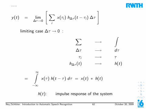
. . .
y(t) = lim∆τ→0
[∑i
x(τi ) h∆τ (t − τi ) ∆τ
]
limiting case ∆τ → 0 : ∑−→
∫∆τ −→ dτ
τi −→ τ
h∆τ (t) −→ h(t)
=
∞∫−∞
x(τ) h(t − τ) dτ = x(t) ∗ h(t)
h(t): impulse response of the system
Ney/Schluter: Introduction to Automatic Speech Recognition 62 October 20, 2009
Examples of LTI-operations:
I Oscillatory systems (electrical or mechanical) with
external excitation: x(t) −→ h(τ) −→ y(t)
y(t) =
∫h(t − τ) x(τ) dτ
y ′′(t) + 2αy ′(t) + β2y(t) = x(t)
α, β: parameters depending on the oscillatory systemI Electrical engineering systems: high-pass, low-pass, band-passI Moving average:
x(t) −→ S −→ y(t) := x(t)
x(t) =1
T
+T/2∫−T/2
x(t + τ) dτ
Ney/Schluter: Introduction to Automatic Speech Recognition 63 October 20, 2009
I Differentiator:
x(t) −→ S −→ y(t) := x ′(t)
I Comb filter: ”hypothesized” period T
x(t) −→ S −→ y(t) := x(t)− x(t − T )
I In general: linear differential equations with coefficients ck , dl :∑k
cky (k)(t) =∑l
dlx(l)(t) [ + further constraints ]
I Example of a non-linear system:
system: y(t) = x2(t)
x(t) = A cos(βt)
=⇒ y(t) = A2 cos2(βt) =A2
2(1 + cos(2βt))
frequency doubling
Ney/Schluter: Introduction to Automatic Speech Recognition 64 October 20, 2009
Outline0. Lehrstuhl fur Informatik 6
1. Introduction to Speech Recognition
2. Digital Signal Processing2.1 Motivation2.2 Linear time-invariant Systems2.3 Fourier Transform2.4 δ-Function2.5 Fourier Series2.6 Discrete Time Signal Processing2.7 Sampling (Nyquist) Theorem and Reconstruction2.8 Fourier Transform and z–Transform2.9 System Representation and Examples2.10 Discrete Time Signal Fourier Transform Theorems2.11 Discrete Fourier Transform (DFT)2.12 Fast Fourier Transform (FFT)
3. Spectral Analysis
4. Time Alignment and Isolated Word Recognition
5. Statistical Interpretation and Models
6. Connected Word Recognition
7. Large Vocabulary Speech Recognition
Ney/Schluter: Introduction to Automatic Speech Recognition 65 October 20, 2009
Fourier Transform
Sinusoidal oscillation:
x(t) = A sin ( ω t + ϕ )
amplitude Aphase / null phase ϕangular frequency ω = 2 π f
dimension:
DIM(ω) DIM(t) = 1
DIM(ω) =1
DIM(t)
=1
[sec]= [Hz]
complex representation:
e j α = cos α + j sin α, α ∈ IRj2 = −1, j ∈ C
cos α =e jα + e−jα
2
sin α =e jα − e−jα
2jcos
sin
αα
α
Im
Re
1
1
Ney/Schluter: Introduction to Automatic Speech Recognition 66 October 20, 2009
LTI-System
y(t) =
∞∫−∞
x(t − τ)h(τ)dτ = x(t) ∗ h(t)
I Determine the following specific input signal:
x(t) = A e j(ωt+ϕ)
I For this input signal the output signal becomes:
y(t) =
∞∫−∞
A e j(ω(t−τ)+ϕ)h(τ)dτ
= A e j(ωt+ϕ)
∞∫−∞
h(τ)e−jωτdτ
︸ ︷︷ ︸H(ω) = F h(τ)
= x(t) · H(ω)
Ney/Schluter: Introduction to Automatic Speech Recognition 67 October 20, 2009
Definition of the Fourier transform:
H(ω) =
∞∫−∞
h(τ)e−jωτdτ = F h(τ) = F τ → h(τ)
(→ decomposition into e−jωτ )
I H(ω) is called transfer function of the system
Remarks about x(t) = A e j(ωt+ϕ):
I The shape of the input signal x(t), i.e. its frequency ω(“eigenfunction”) remains invariant
I Amplitude (intensity) and phase (time shift) are depending onH(ω) (“eigenvalue”)
(→ analogy to the problem of eigenvalues in linear algebra)
Ney/Schluter: Introduction to Automatic Speech Recognition 68 October 20, 2009
RemarksI FT is complex:
H(ω) = Re H(ω) + j Im H(ω) = |H(ω)| e jΦ(ω)
I Amplitude (spectrum):
|H(ω)| =
√Re H(ω)2 + Im H(ω)2
I Phase (spectrum):
Φ(ω) =
arctan
(Im H(ω)Re H(ω)
)Re H(ω) > 0
arctan
(Im H(ω)Re H(ω)
)+ π Re H(ω) < 0
π
2Re H(ω) = 0, Im H(ω) > 0
−π2
Re H(ω) = 0, Im H(ω) < 0
Ney/Schluter: Introduction to Automatic Speech Recognition 69 October 20, 2009
Examples of Fourier transforms1. Rectangle function
h(t) = rect(t
T) =
1, |t| ≤ T/20, |t| > T/2
t
h(t)
H(ω)
ω
H(ω) =
∞∫−∞
h(t)e−jωtdt =
T2∫
−T2
e−jωtdt =1
−jω
[e−jω T
2 − e jω T2
]
=2
ωsin(
ωT
2) =
T sin(ωT
2)
ωT
2
(here: Im H(ω) = 0)
Ney/Schluter: Introduction to Automatic Speech Recognition 70 October 20, 2009
Double-sided exponential
h(t) = e−α|t| with α > 0
H(ω) =
∞∫−∞
h(t)e−jωtdt =
∞∫0
e−(α+jω)tdt +
∞∫0
e−(α−jω)tdt
=
[e−(α+jω)t
−(α + jω)+
e−(α−jω)t
−(α− jω)
]∞0
= 0 + 0− 1
−(α + jω)− 1
−(α− jω)
=α− jω + α + jω
α2 + ω2
=2α
α2 + ω2
Ney/Schluter: Introduction to Automatic Speech Recognition 71 October 20, 2009
h(t) = e−α|t| ↔ H(ω) =2α
α2 + ω2
I Imaginary part equals 0I Infinite spectrumI No zeros
h(t)
t
H( )ω
ω
I If h(t) is symmetric (i.e. h(t) = h(−t)), imaginary parts dropaway and the real part is sufficient
Ney/Schluter: Introduction to Automatic Speech Recognition 72 October 20, 2009
Damped oscillations
h(t) = e−α|t| cos(βt) with α > 0
H(ω) =
∞∫−∞
h(t)e−jωtdt
=
∞∫0
e−(α+jω)t cos(βt)dt +
∞∫0
e−(α−jω)t cos(βt)dt
=
∞∫0
e−(α+jω)t e jβt + e−jβt
2dt +
∞∫0
e−(α−jω)t e jβt + e−jβt
2dt
= . . . (elementary calculation)
=α
α2 + (ω − β)2+
α
α2 + (ω + β)2
Ney/Schluter: Introduction to Automatic Speech Recognition 73 October 20, 2009
I Limiting case: H(ω)|ω=±β =1
α+
α
α2 + (2β)2
=⇒ tends towards ∞ or −∞ if α tends towards 0
ω
H( )ω
β−β| |
h(t)
t
Ney/Schluter: Introduction to Automatic Speech Recognition 74 October 20, 2009
Modulated rectangle function (“truncated cosine”)
h(t) =
cos(β t), |t| ≤ T/2
0, |t| > T/2
H(ω) =
∞∫−∞
h(t)e−jωtdt =
T2∫
−T2
cos(β t)e−jωtdt
= . . . (elementary calculation)
=T
2
sin
((ω − β)
T
2
)(ω − β)
T
2
+
sin
((ω + β)
T
2
)(ω + β)
T
2
Ney/Schluter: Introduction to Automatic Speech Recognition 75 October 20, 2009
| |
h(t)
t
H( )ω
ω
h(t)
t
| |
ω
ωH( )
β−β
rectangle function
modulated rectangle = truncated cosine
Ney/Schluter: Introduction to Automatic Speech Recognition 76 October 20, 2009
Fourier Transform pairs (u = ω/2π)
Rectangle function
1
-1/2 1/2
-1/2 1/2
Triangle function
1
Exponential function
e-α|x|
Gaussian function
e-αx2
Unit impulse
δ(x)
1
Sinc function
Squared sinc function
sin(πu)πu
1
α2+(2πu)2
2α
πu2
αe-πα
1
Rectangle function
1
-1/2 1/2
-1/2 1/2
Triangle function
1
Exponential function
e-α|x|
Gaussian function
e-αx2
Unit impulse
δ(x)
1
Sinc function
Squared sinc function
sin(πu)πu
1
α2+(2πu)2
2α
πu2
αe-πα
1
Ney/Schluter: Introduction to Automatic Speech Recognition 77 October 20, 2009
Fourier Transform pairs (u = ω/2π)
Rectangle function
1
-1/2 1/2
-1/2 1/2
Triangle function
1
Exponential function
e-α|x|
Gaussian function
e-αx2
Unit impulse
δ(x)
1
Sinc function
Squared sinc function
sin(πu)πu
1
α2+(2πu)2
2α
πu2
αe-πα
1
Rectangle function
1
-1/2 1/2
-1/2 1/2
Triangle function
1
Exponential function
e-α|x|
Gaussian function
e-αx2
Unit impulse
δ(x)
1
Sinc function
Squared sinc function
sin(πu)πu
1
α2+(2πu)2
2α
πu2
αe-πα
1
Rectangle function
1
-1/2 1/2
-1/2 1/2
Triangle function
1
Exponential function
e-α|x|
Gaussian function
e-αx2
Unit impulse
δ(x)
1
Sinc function
Squared sinc function
sin(πu)πu
1
α2+(2πu)2
2α
πu2
αe-πα
1
Ney/Schluter: Introduction to Automatic Speech Recognition 78 October 20, 2009
Inverse of Fourier–transform
I Fourier transform (FT):
H(ω) =
∞∫−∞
h(t)e−jωtdt
I assumption for inverse FT:
h(t) =1
2π
∞∫−∞
H(ω)e jωtdω
Ney/Schluter: Introduction to Automatic Speech Recognition 79 October 20, 2009
inserting H(ω) in h(t):
h(t) =1
2πlim
Ω,T→∞
Ω∫−Ω
T∫−T
h(τ) e jω(t−τ) dτ
dω
=1
2πlim
Ω→∞lim
T→∞
T∫−T
Ω∫−Ω
e jω(t−τ) dω h(τ) dτ
= limΩ→∞
limT→∞
1
π
T∫−T
sin (Ω(t − τ))
t − τh(τ) dτ
= limΩ→∞
1
π
∞∫−∞
sin (Ω(t − τ))
t − τh(τ) dτ
= h(t)
Ney/Schluter: Introduction to Automatic Speech Recognition 80 October 20, 2009
due to:
limΩ→∞
1
π
∞∫−∞
sin(Ωt)
th(t) dt = h(0)
formal expression:
h(t) =
∞∫−∞
1
2π
∞∫−∞
e jω(t−τ) dω
︸ ︷︷ ︸
= δ(t − τ)
h(τ) dτ
I δ(t − τ): Dirac delta function
I distribution theory, see there for stronger proof
Ney/Schluter: Introduction to Automatic Speech Recognition 81 October 20, 2009
Outline0. Lehrstuhl fur Informatik 6
1. Introduction to Speech Recognition
2. Digital Signal Processing2.1 Motivation2.2 Linear time-invariant Systems2.3 Fourier Transform2.4 δ-Function2.5 Fourier Series2.6 Discrete Time Signal Processing2.7 Sampling (Nyquist) Theorem and Reconstruction2.8 Fourier Transform and z–Transform2.9 System Representation and Examples2.10 Discrete Time Signal Fourier Transform Theorems2.11 Discrete Fourier Transform (DFT)2.12 Fast Fourier Transform (FFT)
3. Spectral Analysis
4. Time Alignment and Isolated Word Recognition
5. Statistical Interpretation and Models
6. Connected Word Recognition
7. Large Vocabulary Speech Recognition
Ney/Schluter: Introduction to Automatic Speech Recognition 82 October 20, 2009
Starting point: definition of the δ-function as aboundary case of a function δε(t):
limε→0
+∞∫−∞
f (t) δε(t) dt = f (0) (3.1)
I Possible realizations of δε(t)
a) δε(t) =
1
2εt ∈ [−ε,+ε]
0 otherwise
b) δε(t) =1
π
ε
ε2 + t2
c) δε(t) =1
π
sin (t/ε)
t
d) δε(t) =1√
2πε2e−
t2
2ε2
Ney/Schluter: Introduction to Automatic Speech Recognition 83 October 20, 2009
I During inversion of the Fourier transformwe have “formally” obtained:
δ(t) =1
2π
+∞∫−∞
e jωt dω = limΩ→∞
1
π
sin (Ωt)
t(3.2)
Fourier transform Fδ(t):
Fδ(t) =
+∞∫−∞
e−jωtδ(t) dt
due to (3.1) the following holds:
Fδ(t) = e jωt |t=0 = 1
Ney/Schluter: Introduction to Automatic Speech Recognition 84 October 20, 2009
I Another derivation using (3.2):
δ(t) =1
2π
+∞∫−∞
e jωt Fδ(t) dω general
=1
2π
+∞∫−∞
e jωt dω according to (3.2)
Comparison results in:
Fδ(t) = 1
Ney/Schluter: Introduction to Automatic Speech Recognition 85 October 20, 2009
From this we obtain the following equations:
From symmetry property:
F1 = 2 π δ(ω)
From shifting theorem:
Fe jω0t = 2 π δ(ω − ω0)
Ney/Schluter: Introduction to Automatic Speech Recognition 86 October 20, 2009
cos (ω0 t) =1
2
[e jω0t + e−jω0t
]=
1
2
+∞∫−∞
δ(ω − ω0) e jωt dω +
+∞∫−∞
δ(ω + ω0) e jωt dω
= π
1
2π
+∞∫−∞
[ δ(ω − ω0) + δ(ω + ω0) ] e jωt dω
F cos (ω0 t) = π [ δ(ω − ω0) + δ(ω + ω0) ]
Ney/Schluter: Introduction to Automatic Speech Recognition 87 October 20, 2009
Note another derivation:
consider “damped oscillations”
1
2πe−α|t| cos (ω0t)
in the limit α→ 0 .
Ney/Schluter: Introduction to Automatic Speech Recognition 88 October 20, 2009
Comb function
I define “comb function” (pulse train, sequence of δ-impulses):
x(t) =+∞∑
n=−∞δ(t − nT )
Ney/Schluter: Introduction to Automatic Speech Recognition 89 October 20, 2009
I Fourier transform of comb function:
X (ω) =
+∞∫−∞
x(t) e−jωt dt
=
+∞∫−∞
+∞∑n=−∞
δ(t − nT ) e−jωt dt
=+∞∑
n=−∞
+∞∫−∞
δ(t − nT ) e−jωt dt
=+∞∑
n=−∞e−jωnT
= . . . (see Papoulis 1962, p. 44)
=2π
T
+∞∑n=−∞
δ(ω − n2π
T)
Ney/Schluter: Introduction to Automatic Speech Recognition 90 October 20, 2009
I in words:
δ-impulse sequence with period T in time domain
produces
δ-impulse sequence with period 1T in frequency domain
(i.e. 2πT in ω-frequency domain)
comb function is transformed to comb function
Ney/Schluter: Introduction to Automatic Speech Recognition 91 October 20, 2009
Comb function
cos(ω0t)
sin(ω0t)
-2π-4π-6π 2π 4π 6πT T T T T T
T 3T-T-3T 6T-6T
δ(t-nT)Σn=-
12j(−δ(ω-ω0)+δ(ω+ω0))
(δ(ω-ω0)+δ(ω+ω0))12
Σ δ(ω-n2π/T)n=-
2πT
−ω0 ω0
−ω0
ω0
Comb function
cos(ω0t)
sin(ω0t)
-2π-4π-6π 2π 4π 6πT T T T T T
T 3T-T-3T 6T-6T
δ(t-nT)Σn=-
12j(−δ(ω-ω0)+δ(ω+ω0))
(δ(ω-ω0)+δ(ω+ω0))12
Σ δ(ω-n2π/T)n=-
2πT
−ω0 ω0
−ω0
ω0
Comb function
cos(ω0t)
sin(ω0t)
-2π-4π-6π 2π 4π 6πT T T T T T
T 3T-T-3T 6T-6T
δ(t-nT)Σn=-
12j(−δ(ω-ω0)+δ(ω+ω0))
(δ(ω-ω0)+δ(ω+ω0))12
Σ δ(ω-n2π/T)n=-
2πT
−ω0 ω0
−ω0
ω0
Ney/Schluter: Introduction to Automatic Speech Recognition 92 October 20, 2009
Properties of the Fourier TransformSymmetry
H(ω) =
∞∫−∞
h(t) e−jωt dt = F h(t)
h(t) =1
2π
∞∫−∞
H(ω) e jωt dω = F−1 H(ω)
F 2h(t) = FH(ω) = 2πh(−t)
F−1 Fh(t) = F−1H(ω) = h(t)
I Time domain and frequency domain are correlatedsymmetrically.
I Properties of FT are valid in both domains, especially theconvolution theorem (see later).
Ney/Schluter: Introduction to Automatic Speech Recognition 93 October 20, 2009
Theorems for the Fourier transform
H(ω) =
∞∫−∞
e−jωt h(t) dt
consider the equation:
H(ω) = F h(t)
more exact:
ω → H(ω) = F t → h(t)
Ney/Schluter: Introduction to Automatic Speech Recognition 94 October 20, 2009
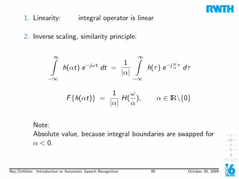
1. Linearity: integral operator is linear
2. Inverse scaling, similarity principle:
∞∫−∞
h(αt) e−jωt dt =1
|α|
∞∫−∞
h(τ) e−j ωατ dτ
Fh(αt) =1
|α|H(ω
α), α ∈ IR\0
Note:Absolute value, because integral boundaries are swapped forα < 0.
Ney/Schluter: Introduction to Automatic Speech Recognition 95 October 20, 2009
3. Shift: h(t − t0)∞∫−∞
h(t − t0) e−jωt dt = e−jωt0
∞∫−∞
h(t − t0) e−jω(t−t0) dt
= e−jωt0
∞∫−∞
h(τ) e−jωτ dτ
=⇒ Fh(t − t0) = e−jωt0H(ω) t0 ∈ IR
with H(ω) = Fh(t)important:
| Fh(t − t0) | = | Fh(t) |,
since: |e−jωt0 | = |e−ju| = | cos u − j sin u|=
√cos2 u + sin2u = 1
Ney/Schluter: Introduction to Automatic Speech Recognition 96 October 20, 2009
4. Symmetry and antisymmetry:
h(t) = h(−t) ⇒ ImH(ω) = 0
h(t) =−h(−t) ⇒ ReH(ω) = 0
5. Complex conjugation: assume h(t) to be a complex function
Ney/Schluter: Introduction to Automatic Speech Recognition 101 October 20, 2009
FourierTransform
Convolution with h(t)
Multiplication with H(ω) = Fh(t)
Inverse FourierTransform
x(t)
X(ω)
y(t)
Y(ω)
I Motivation for the Fourier transform:FT gives the “simplest” representation of the systemoperation, because every LTI-System can be interpreted asconvolution of the input signal x(t) and the impulse responseof the system h(t). Convolution can be then efficientlycalculated using FT and convolution theorem.
I Mathematical: eigenfunctionsNey/Schluter: Introduction to Automatic Speech Recognition 102 October 20, 2009
Example: Oscillator with excitation
x(t) −→ Oscillator −→ y(t)
y ′′(t) + 2α y ′(t) + β2 y(t) = x(t)
x(t) =1
2π
+∞∫−∞
X (ω)e jωtdω
y(t) =1
2π
+∞∫−∞
Y (ω)e jωtdω
y ′(t) =1
2π
+∞∫−∞
Y (ω)jω e jωtdω
y ′′(t) =1
2π
+∞∫−∞
Y (ω)[−ω2] e jωtdω
Ney/Schluter: Introduction to Automatic Speech Recognition 103 October 20, 2009
Substitute x(t),y(t),y ′(t),and y ′′(t) into oscillator differentialequation:
+∞∫−∞
[−ω2 + 2αjω + β2]Y (ω)e jωtdω =
+∞∫−∞
X (ω)e jωtdω
⇔+∞∫−∞
[−ω2 + 2αjω + β2] Y (ω)− X (ω)
︸ ︷︷ ︸=0
e jωtdω = 0 ∀t
In this way we obtain the transfer function of an oscillator:
H(ω) =Y (ω)
X (ω)=
1
−ω2 + 2αjω + β2
Ney/Schluter: Introduction to Automatic Speech Recognition 104 October 20, 2009
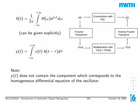
h(t) =1
2π
+∞∫−∞
H(ω)e jωtdω
(can be given explicitly)
y(t) =
+∞∫−∞
x(t) h(t − τ)dτ
FourierTransform
Convolution with h(t)
Multiplication with H(ω) = Fh(t)
Inverse FourierTransform
x(t)
X(ω)
y(t)
Y(ω)
Note:y(t) does not contain the component which corresponds to thehomogeneous differential equation of the oscillator.
Ney/Schluter: Introduction to Automatic Speech Recognition 105 October 20, 2009
Parseval Theorem
Convolution theorem:
F−1 H(ω) X (ω) =
∞∫−∞
h(t) x(τ − t) dt
⇔ 1
2π
∞∫−∞
H(ω) X (ω) e jωτ dω = (h ∗ x) (τ) (?)
We make two special assumptions:
i) x(−t) := h(t), then: X (ω) = H(ω)
ii) τ = 0
Ney/Schluter: Introduction to Automatic Speech Recognition 106 October 20, 2009
Inserting i) and ii) in (?) results in the Parseval Theorem:
1
2π
∞∫−∞
H(ω)H(ω) dω =
∞∫−∞
h(t)h(t) dt
=1
2π
∞∫−∞
|H(ω)|2 dω =
∞∫−∞
|h(t)|2 dt = E
I Energy E in time domain = Energy E in frequency domain
(up to the factor1
2π; aid: use normalization factor
1√2π
for
both directions of Fourier Transform)
I Physical aspect: energy conservation
I Mathematical aspect: unitary (orthogonal) representation invector space
I |H(ω)|2 is called power spectral density.
Ney/Schluter: Introduction to Automatic Speech Recognition 107 October 20, 2009
Outline0. Lehrstuhl fur Informatik 6
1. Introduction to Speech Recognition
2. Digital Signal Processing2.1 Motivation2.2 Linear time-invariant Systems2.3 Fourier Transform2.4 δ-Function2.5 Fourier Series2.6 Discrete Time Signal Processing2.7 Sampling (Nyquist) Theorem and Reconstruction2.8 Fourier Transform and z–Transform2.9 System Representation and Examples2.10 Discrete Time Signal Fourier Transform Theorems2.11 Discrete Fourier Transform (DFT)2.12 Fast Fourier Transform (FFT)
3. Spectral Analysis
4. Time Alignment and Isolated Word Recognition
5. Statistical Interpretation and Models
6. Connected Word Recognition
7. Large Vocabulary Speech Recognition
Ney/Schluter: Introduction to Automatic Speech Recognition 108 October 20, 2009
Fourier Seriesx : IR −→ IR
t −→ x(t)
Consider a periodical function x with period T :
x(t) = x(t + T ) for each t ∈ IRthen also x(t) = x(t + kT ) for k ∈ Z
Examples:I Constant function:
x0(t) = A0
I Harmonic oscillator:
x1(t) = A1 cos (2π
Tt + ϕ1) , A1 > 0
I All higher harmonics:
xn(t) = An cos (n2π
Tt + ϕn) , An > 0
Ney/Schluter: Introduction to Automatic Speech Recognition 109 October 20, 2009
therefore
x(t) =∞∑
n=0
An cos (n ω0 t + ϕn) with ω0 =2 π
T, An ≥ 0
is periodical with period T = 2πω0
I Another notation:
x(t) =∞∑
n=−∞Bn e−j n ω0 t where Bn is a complex number
Line spectrumrepresentation:
Ney/Schluter: Introduction to Automatic Speech Recognition 110 October 20, 2009
A real measured signal has always a ”widespread” spectrum.
Reasons:I Strictly periodical signal (almost) never exists
I Period can fluctuateI ”Wave form” within one period can fluctuateI Only a finite section of the signal is analyzed
(”window function”)
I Only a strictly periodical signal has a sharp line spectrum
Remarks:
I Fourier series are actually not strictly related to periodicalfunctions: a finite interval of IR is sufficient (the signal is theninterpreted as infinitely prolonged).
I By transition from the finite interval to the complete real axisthe Fourier series becomes Fourier integral.
Ney/Schluter: Introduction to Automatic Speech Recognition 111 October 20, 2009
Calculation of Fourier coefficient
I Consider a periodical function x(t) with period T = 2πω0
I approach:
x(t) =+∞∑
n=−∞an e j nω0 t a ∈ C
I multiplication with e−j mω0 t where m ∈ IN and integrationover one period result in:
+T/2∫−T/2
x(t) e−j m ω0 t dt =+∞∑
n=−∞an
+T/2∫−T/2
e j (n−m) ω0 t dt
Ney/Schluter: Introduction to Automatic Speech Recognition 112 October 20, 2009
I Due to “orthogonality” holds:
+T/2∫−T/2
e j (n−m) ω0 t dt =
T if n = m0 if n 6= m
I Then:T/2∫−T/2
x(t) e−j m ω0 t dt = am T
I Result:
an =1
T
+T/2∫−T/2
x(t) e−j n ω0 t dt
=1
T
+T/2∫−T/2
x(t) cos (n ω0 t) dt − j1
T
+T/2∫−T/2
x(t) sin (n ω0 t) dt
Ney/Schluter: Introduction to Automatic Speech Recognition 113 October 20, 2009
Spectrum of a periodical function
I If x(t) is periodical with the period T = 2πω0
, then
x(t) =+∞∑
n=−∞an e j nω0 t , an ∈ C
I The Fourier transform X (ω) is:
X (ω) = Fx(t)
=+∞∑
n=−∞an Fe j n ω0 t︸ ︷︷ ︸
= 2πδ(ω − nω0)
= 2 π+∞∑
n=−∞an δ(ω − nω0)
Ney/Schluter: Introduction to Automatic Speech Recognition 114 October 20, 2009
I Note:This derivation is formal, because the Fourier integral does notexist in the “usual sense”;strict derivation within the scope of distribution theory.
I In words:a periodic function with the period T has a Fourier transformin the form of a line spectrum with the distance ω0 = 2π
Tbetween the components.
Ney/Schluter: Introduction to Automatic Speech Recognition 115 October 20, 2009
Outline0. Lehrstuhl fur Informatik 6
1. Introduction to Speech Recognition
2. Digital Signal Processing2.1 Motivation2.2 Linear time-invariant Systems2.3 Fourier Transform2.4 δ-Function2.5 Fourier Series2.6 Discrete Time Signal Processing2.7 Sampling (Nyquist) Theorem and Reconstruction2.8 Fourier Transform and z–Transform2.9 System Representation and Examples2.10 Discrete Time Signal Fourier Transform Theorems2.11 Discrete Fourier Transform (DFT)2.12 Fast Fourier Transform (FFT)
3. Spectral Analysis
4. Time Alignment and Isolated Word Recognition
5. Statistical Interpretation and Models
6. Connected Word Recognition
7. Large Vocabulary Speech Recognition
Ney/Schluter: Introduction to Automatic Speech Recognition 116 October 20, 2009
Discrete Time Signal ProcessingIf we want to process a continuous time signal x(t) with acomputer, we have to sample it at discrete equidistant time points
tn = n · TS
where TS is called sampling period.
Ney/Schluter: Introduction to Automatic Speech Recognition 117 October 20, 2009
Terminology:
I “time discrete” is often called “digital”, where this adjectiveoften (but not always) denotes the amplitude quantization,i.e. the quantization of the value x(n · TS).
Advantages of digital processing in comparison to analog components:
I independent of analog components and technicaldifficulties with respect to their realization;
I in principle arbitrary high accuracy;
I also non-linear methods are possible,in principle even every mathematical method.
Ney/Schluter: Introduction to Automatic Speech Recognition 118 October 20, 2009
Digital Simulation using Discrete Time SystemsTask definition:
I Given:Analog system with input signal x(t) and output signal y(t);Sampling with sampling period TS
I Wanted:Discrete System with input signal x [n] and output signal y [n],such that
x [n] = x(nTS)
results in
y [n] = y(nTS)
I For which signals is such a digital simulation possible?
I The sampling theorem gives (most of) the answer.
Ney/Schluter: Introduction to Automatic Speech Recognition 119 October 20, 2009
LTI System (analog to continuous time case):
I Linearity:
I Homogeneity:
S α x [n] = α S x [n]
I Additivity:
S x1[n] + x2[n] = S x1[n] + S x2[n]
I Shift invariance:
S x [n − n0] = y [n − n0], n0 whole number
Ney/Schluter: Introduction to Automatic Speech Recognition 120 October 20, 2009
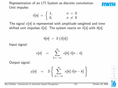
Representation of an LTI System as discrete convolution:Unit impulse:
δ[n] =
1, n = 00, n 6= 0
The signal x [n] is represented with amplitude weighted and timeshifted unit impulses δ[n]. The system reacts on δ[n] with h[n]:
h[n] = S δ[n]
Input signal:
x [n] =∞∑
k=−∞x [k] δ[n − k]
Output signal:
y [n] = S
∞∑k=−∞
x [k] δ[n − k]
Ney/Schluter: Introduction to Automatic Speech Recognition 121 October 20, 2009
Additivity
=∞∑
k=−∞S x [k] δ[n − k]
Homogeneity
=∞∑
k=−∞x [k] S δ[n − k]
Time invariance
=∞∑
k=−∞x [k] h[n − k]
I Input signal x [n] and output signal y [n] of a discrete time LTIsystem are linked through discrete convolution.
I h[n] is called impulse response like in continuous time case.
Ney/Schluter: Introduction to Automatic Speech Recognition 122 October 20, 2009
Examples of Discrete Time Systems
I Difference calculation:
y [n] = x [n] − x [n − n0]
I First order difference equation:(recursive averaging, averaging with memory)
y [n]− α y [n − 1] = x [n]
I (Digital) resonator (second order difference equation)
y [n]− α y [n − 1]− β y [n − 2] = x [n]
Ney/Schluter: Introduction to Automatic Speech Recognition 123 October 20, 2009
I “1-2-1”-averaging:
y [n] = 0.5 · x [n − 1] + x [n] + 0.5 · x [n + 1]
I sliding window averaging (“smoothing”)
y [n] =1
2M + 1
M∑k=−M
x [n − k]
I weighted averaging: instead of constant weight
h[n] =1
2M + 1
arbitrary weights can be used:
y [n] =M∑
k=−M
h[k] · x [n − k]
Note: the only difference from general case isfinite length of the convolution kernel h[n].
Ney/Schluter: Introduction to Automatic Speech Recognition 124 October 20, 2009
Outline0. Lehrstuhl fur Informatik 6
1. Introduction to Speech Recognition
2. Digital Signal Processing2.1 Motivation2.2 Linear time-invariant Systems2.3 Fourier Transform2.4 δ-Function2.5 Fourier Series2.6 Discrete Time Signal Processing2.7 Sampling (Nyquist) Theorem and Reconstruction2.8 Fourier Transform and z–Transform2.9 System Representation and Examples2.10 Discrete Time Signal Fourier Transform Theorems2.11 Discrete Fourier Transform (DFT)2.12 Fast Fourier Transform (FFT)
3. Spectral Analysis
4. Time Alignment and Isolated Word Recognition
5. Statistical Interpretation and Models
6. Connected Word Recognition
7. Large Vocabulary Speech Recognition
Ney/Schluter: Introduction to Automatic Speech Recognition 125 October 20, 2009
Sampling (Nyquist) Theorem and ReconstructionThe following will be analyzed and derived respectively:How should we choose the sampling period TS , if we want torepresent a continuous signal x(t) with its sample values x(nTS)so that the signal x(t) can be exactly reconstructed from itssample values?
I Fourier transform of the continuous time signal x(t):
X (ω) = F x(t) =
∞∫−∞
x(t) e−jωt dt
x(t) = F−1 X (ω) =1
2π
∞∫−∞
X (ω) e jωt dω (3.3)
I Signal x(t) has limited bandwidth with upper limit ωB , whichmeans: X (ω) = 0 for all |ω| ≥ ωB
Note: X (ωB) = 0
Ney/Schluter: Introduction to Automatic Speech Recognition 126 October 20, 2009
I X (ω) in domain −ωB < ω < ωB can be represented asFourier Series:
X (ω) =∞∑
n=−∞an exp(−jnπ
ω
ωB) (3.4)
I The coefficients an are given by:
an =1
2ωB
ωB∫−ωB
X (ω) exp(jnπω
ωB) dω (3.5)
I Comparison of the Eqs. (3.3) and (3.5) shows that thecoefficients an are given by the values of the inverse Fouriertransform of x(t) at points
tn =nπ
ωB
The band limitation of X (ω) has to be considered for theintegration limits in (3.3). Result:
an = x(nπ
ωB) · πωB
(3.6)
Ney/Schluter: Introduction to Automatic Speech Recognition 127 October 20, 2009
I Inserting Eq. (3.6) into Eq. (3.4) and then in Eq. (3.3)results in:
x(t) =1
2π
ωB∫−ωB
π
ωB
∞∑n=−∞
x(nπ
ωB) exp(−jnπ
ω
ωB) exp(jωt) dω
I Swap summation and integration and carry out integration:
x(t) =∞∑
n=−∞x(
nπ
ωB)
sin(ωB (t − nπ
ωB))
ωB (t − nπ
ωB)
I Reconstruction of the signal x(t) from sample values is
possible if equidistant sample values x(nπ
ωB) = x(n · Ts) have
the distanceTS =
π
ωB(3.7)
Ney/Schluter: Introduction to Automatic Speech Recognition 128 October 20, 2009
I The sampling period TS corresponds to the samplingfrequency ΩS :
ΩS =2π
TS
I Eq. (3.7) shows that if the sampling frequency is
ΩS := 2 ωB
the original signal x(t) can be reconstructed exactly.
I In the Fourier series representation of X (ω) in Eq. (3.4), theperiod 2 · ωB has been supposed.
ωB is the highest frequency component of the signal x(t).
Ney/Schluter: Introduction to Automatic Speech Recognition 129 October 20, 2009
I Since X (ω) is equal to zero for |ω| ≥ ωB , the period 2 · ωB
can be substituted with every period 2 · ωB where ωB ≥ ωB .The previous derivation is also valid for this ωB .
I When
ωB =π
TS
then:
x(t) =∞∑
n=−∞x(n TS)
sin(π (t − n TS)/TS)
π (t − n TS)/TS
(reconstruction formula)
Note: limt→0sin(t)
t = 1 (l’Hopital’s rule)
Ney/Schluter: Introduction to Automatic Speech Recognition 130 October 20, 2009
I The condition ωB ≥ ωB results in:
TS ≤π
ωB(3.8)
for the sampling period TS and in:
ΩS ≥ 2 · ωB (3.9)
for the sampling frequency ΩS .
I The Eqs. (3.8) and (3.9) are denoted as sampling theorem.
The sampling frequency has to be at least twice as high as theupper limit frequency of the signal ωB where X (ω) = 0 for|ω| ≥ ωB .
If and only if this condition is satisfied, an exactreconstruction (without approximation!) of a continuoussignal x(t) from its sample values x(nTS) is possible.
I Note: The sampling frequency ΩS = 2 · ωB is also called
Nyquist frequency.
Ney/Schluter: Introduction to Automatic Speech Recognition 131 October 20, 2009
Ideal Reconstruction
t
x(t)
t
xs(t)
xr(t)
T
T
a)
b)
c)
t
x(t)
t
xs(t)
xr(t)
T
T
a)
b)
c)
t
x(t)
t
xs(t)
xr(t)
T
T
a)
b)
c)
Figure: Ideal reconstruction of a band-limited signal (from Oppenheim,Schafer): a) original signal b) sampled signal c) reconstructed signal
Ney/Schluter: Introduction to Automatic Speech Recognition 132 October 20, 2009
AliasingX(ω)
ωωΒ−ωΒ
a)
ωωΒ−ωΒ
b)
-ΩS ΩS
. . . . . .
XS1(ω) ΩS > 2ωΒ,
XS2(ω)
ωωΒ−ωΒ
c)
, ΩS = 2ωΒ
-ΩS ΩS
. . . . . .
(Nyquist rate)
XS3(ω)
ωΒ−ωΒ
, ΩS < 2ωΒ (aliasing)
. . . . . .
ΩS−ΩS
d)
ω
a) original spectrum
X(ω)
ωωΒ−ωΒ
a)
ωωΒ−ωΒ
b)
-ΩS ΩS
. . . . . .
XS1(ω) ΩS > 2ωΒ,
XS2(ω)
ωωΒ−ωΒ
c)
, ΩS = 2ωΒ
-ΩS ΩS
. . . . . .
(Nyquist rate)
XS3(ω)
ωΒ−ωΒ
, ΩS < 2ωΒ (aliasing)
. . . . . .
ΩS−ΩS
d)
ω
b) sampling rate higherthan Nyquist rate:exact reconstructionpossible
X(ω)
ωωΒ−ωΒ
a)
ωωΒ−ωΒ
b)
-ΩS ΩS
. . . . . .
XS1(ω) ΩS > 2ωΒ,
XS2(ω)
ωωΒ−ωΒ
c)
, ΩS = 2ωΒ
-ΩS ΩS
. . . . . .
(Nyquist rate)
XS3(ω)
ωΒ−ωΒ
, ΩS < 2ωΒ (aliasing)
. . . . . .
ΩS−ΩS
d)
ω
c) sampling rate equal toNyquist rate: exactreconstruction possible
X(ω)
ωωΒ−ωΒ
a)
ωωΒ−ωΒ
b)
-ΩS ΩS
. . . . . .
XS1(ω) ΩS > 2ωΒ,
XS2(ω)
ωωΒ−ωΒ
c)
, ΩS = 2ωΒ
-ΩS ΩS
. . . . . .
(Nyquist rate)
XS3(ω)
ωΒ−ωΒ
, ΩS < 2ωΒ (aliasing)
. . . . . .
ΩS−ΩS
d)
ω
Sampling of band-limited signal withdifferent sampling rates.
Ney/Schluter: Introduction to Automatic Speech Recognition 133 October 20, 2009
Another proof using delta- and comb-function:Sampling of the continuous signal x(t) with ΩS = 2π
TS
I Band limitation: X (ω) = 0 for |ω| ≥ ωB
(always possible: analog to low-pass with T (ω) = 0 for |ω| ≥ ωB)I Sampling procedure
= multiplication with comb function in time domain
xs(t) = Ts x(t) ·+∞∑
n=−∞δ(t − nTs)
= convolution with comb function in frequency domain:
Xs(ω) = Ts ·1
2πX (ω) ∗ 2π
Ts
+∞∑n=−∞
δ
(ω − 2πn
Ts
)
=
+∞∫−∞
X (ω)+∞∑
n=−∞δ
(ω −
[ω − 2πn
Ts
])d ω
=+∞∑
n=−∞X
(ω − n
2π
Ts
)Ney/Schluter: Introduction to Automatic Speech Recognition 134 October 20, 2009
I sampled signal has periodical Fourier spectrum(Analogy to Fourier series: periodical signal has line spectrum,i.e. discrete spectrum)No overlap if:
ωB ≤ ΩS − ωB
2ωB ≤ ΩS
I In so-called digital simulation, the signal x(t) is representedby its sampled values x(n · TS) measured at equidistant timepoints with distance TS . With a proper sampling period TS
an exact reconstruction of the signal x(t) from the sampledvalues x(n · TS) is possible.
I If it is possible to exactly reconstruct the signal x(t) from thesampled values x(n · TS), then it is possible to performdiscrete time processing of the sampled values x(n · TS) on acomputer, which is equivalent to continuous time processingof the signal x(t) (digital simulation).
Ney/Schluter: Introduction to Automatic Speech Recognition 135 October 20, 2009
I Continuous time processing:
y(t) =
∞∫−∞
x(τ) h(t − τ) dτ
I Discrete time processing:I Sampling period TS
I x [n] := x(nTS)
y(nTS) =∞∑
k=−∞x(kTS) h(nTS − kTS) TS , h[n] := TS h(nTS)
y [n] =∞∑
k=−∞x [k] h[n − k]
I Proof: substitute perfect reconstruction of integrand.I As a result of the convolution theorem (convolution in time
domain corresponds to multiplication in frequency domain),the band limited input signal gives an also band limited outputsignal which is exactly determined by its sampled values.
Ney/Schluter: Introduction to Automatic Speech Recognition 136 October 20, 2009
Important (cf. derivation of Nyquist theorem):I In the domain |ω| < ΩS/2 the Fourier transform of a
continuous time signal x(t) is identical with theFourier–transform of the corresponding sampled discrete timesignal x(nTS):
X (ω) =
∞∫−∞
x(t) exp(−jωt) dt
for |ω| ≤ ΩS/2 is identical to
TS · XS(ω) = TS ·∞∑
n=−∞x(nTS) exp(−jωTSn)
= TS ·∞∑
n=−∞x(nTS) exp(−j
2πω
ΩSn)
I Inverse Fourier transform of discrete time signal:
x(nTS) =1
ΩS
ΩS/2∫−ΩS/2
XS(ω) exp(jωTSn) dω
Ney/Schluter: Introduction to Automatic Speech Recognition 137 October 20, 2009
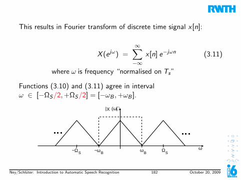
I One period:
−ΩS
2≤ ω ≤ ΩS
2
−π ≤ 2πω
ΩS≤ π
I The Fourier transform of a discrete time signal is periodic in ωwith the period 2π/TS = ΩS .
I The Fourier transform of a discrete time signal iscontinuous in ω.
Ney/Schluter: Introduction to Automatic Speech Recognition 138 October 20, 2009
Frequency normalization
I Define the normalized frequency ωN :
ωN : = 2πω
ΩS
I Definition: (ω now denotes a normalized frequency)
I Fourier transform of discrete time signal x [n]:
X (e jω) =+∞∑
n=−∞x [n] exp(−jωn)
Note the notation X (e jω).
I Inverse Fourier transform of discrete time signal x [n]:
x [n] =1
2π
π∫−π
X (e jω) exp(jωn) dω
Ney/Schluter: Introduction to Automatic Speech Recognition 139 October 20, 2009
Outline0. Lehrstuhl fur Informatik 6
1. Introduction to Speech Recognition
2. Digital Signal Processing2.1 Motivation2.2 Linear time-invariant Systems2.3 Fourier Transform2.4 δ-Function2.5 Fourier Series2.6 Discrete Time Signal Processing2.7 Sampling (Nyquist) Theorem and Reconstruction2.8 Fourier Transform and z–Transform2.9 System Representation and Examples2.10 Discrete Time Signal Fourier Transform Theorems2.11 Discrete Fourier Transform (DFT)2.12 Fast Fourier Transform (FFT)
3. Spectral Analysis
4. Time Alignment and Isolated Word Recognition
5. Statistical Interpretation and Models
6. Connected Word Recognition
7. Large Vocabulary Speech Recognition
Ney/Schluter: Introduction to Automatic Speech Recognition 140 October 20, 2009
Fourier Transform and z–TransformTransfer function and Fourier transformEigenfunctions of discrete linear time invariant systems (analog totime continuous case; ω is dimensionless here):
x [n] = e j ω n −∞ < n < ∞Proof:
y [n] =∞∑
k=−∞h[k] x [n − k] =
∞∑k=−∞
h[k] e j ω (n−k)
= e j ω n∞∑
k=−∞h[k] e−j ω k
Define: H(e j ω) =∞∑
k=−∞h[k] e−j ω k
Remark:The Fourier transform of a discrete time signal is alreadyintroduced as Fourier series during the derivation of samplingtheorem and reconstruction formula, cf. Eq. (3.4).Result: y [n] = e j ω n H(e j ω)
Ney/Schluter: Introduction to Automatic Speech Recognition 141 October 20, 2009
z–transform
I Fourier transform of a discrete time signal x [n]:
X (e jω) =+∞∑
n=−∞x [n] e−jωn
I periodic in ωI ω is normalized frequency, thence:
−π < ω ≤ π
I X is evaluated on the unit circle (e jω)
I Generalization: X is evaluated for any complex values z .
I That results in the z–transform:
X (z) =+∞∑
n=−∞x [n] z−n
Ney/Schluter: Introduction to Automatic Speech Recognition 142 October 20, 2009
I Reasons for z–transform
1. analytically simpler, function theory methods are applicable2. better handling of convergence problem:
I convergence of finite signal, i.e. x [n] = 0 for each n > N0
I convergence of infinite signal depends on z
I Inverse z–transform:
x [n] =1
2πj
∮X (z) zn−1 dz
formally: z = e jω dz = jzdω
x [n] =1
2π
2π∫0
X (e jω) e jωn dω
Ney/Schluter: Introduction to Automatic Speech Recognition 143 October 20, 2009
Example of Fourier transform and z–transform:
I “Truncated geometric series”
x [n] =
an 0 ≤ n ≤ N − 10 otherwise
I z–transform
X (z) =N−1∑n=0
an z−n =N−1∑n=0
(a z−1)n
=1− (a z−1)N
1− a z−1
=1
zN−1
zN − aN
z − a
Ney/Schluter: Introduction to Automatic Speech Recognition 144 October 20, 2009
I Fourier transformz–transform results in Fourier transformation usingsubstitution:
z = e jω
X (e jω) =1− aN e−jωN
1− a e−jω
special case for a = 1 (discrete time rectangle):
= exp
(−jω(N − 1)
2
) sin
(ωN
2
)sin(ω
2
)Ney/Schluter: Introduction to Automatic Speech Recognition 145 October 20, 2009
Proof for the z–transform inversion
I Statement:
x [k] =1
2πj
∮X (z) zk−1 dz
I Cauchy integration rule
1
2πj
∮z−kdz =
1 k = 10 k 6= 1
1
2πj
∮X (z) zk−1dz =
1
2πj
∮ ∑n
x [n] z−n+k−1dz
=∑n
x [n]1
2πj
∮z−n+k−1dz︸ ︷︷ ︸
6= 0 only for n = k
= x [k]
Ney/Schluter: Introduction to Automatic Speech Recognition 146 October 20, 2009
I Fourier case:
z = e jω =⇒ dz = j e jω dω
Then:
x [n] =1
2πj
+π∫−π
X (e jω) (e jω)n−1 j e jωdω
Integration path is unit circle because of e jω
=1
2π
+π∫−π
X (e jω) e jωn dω
Ney/Schluter: Introduction to Automatic Speech Recognition 147 October 20, 2009
Outline0. Lehrstuhl fur Informatik 6
1. Introduction to Speech Recognition
2. Digital Signal Processing2.1 Motivation2.2 Linear time-invariant Systems2.3 Fourier Transform2.4 δ-Function2.5 Fourier Series2.6 Discrete Time Signal Processing2.7 Sampling (Nyquist) Theorem and Reconstruction2.8 Fourier Transform and z–Transform2.9 System Representation and Examples2.10 Discrete Time Signal Fourier Transform Theorems2.11 Discrete Fourier Transform (DFT)2.12 Fast Fourier Transform (FFT)
3. Spectral Analysis
4. Time Alignment and Isolated Word Recognition
5. Statistical Interpretation and Models
6. Connected Word Recognition
7. Large Vocabulary Speech Recognition
Ney/Schluter: Introduction to Automatic Speech Recognition 148 October 20, 2009
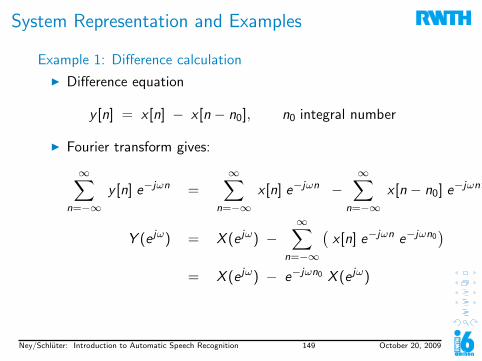
System Representation and Examples
Example 1: Difference calculation
I Difference equation
y [n] = x [n] − x [n − n0], n0 integral number
I Fourier transform gives:
∞∑n=−∞
y [n] e−jωn =∞∑
n=−∞x [n] e−jωn −
∞∑n=−∞
x [n − n0] e−jωn
Y (e jω) = X (e jω) −∞∑
n=−∞
(x [n] e−jωn e−jωn0
)= X (e jω) − e−jωn0 X (e jω)
Ney/Schluter: Introduction to Automatic Speech Recognition 149 October 20, 2009
I Then follows:H(e jω) =
Y (e jω)
X (e jω)
= 1 − e−jωn0
|H(e jω)|2 = (1− cos(ωn0))2 + sin2(ωn0)
= 1 − 2cos(ωn0) + cos2(ωn0) + sin2(ωn0)
= 2 (1 − cos(ωn0))
|H(e iω)|2
0
1
2
3
4
5
ω πn0
Ney/Schluter: Introduction to Automatic Speech Recognition 150 October 20, 2009
Example 2: First order difference equation
Delay
y[n]
x[n]
+
y[n-1]
α
x [n] + α y [n − 1] = y [n]
⇐⇒ y [n] − α y [n − 1] = x [n]
Ney/Schluter: Introduction to Automatic Speech Recognition 151 October 20, 2009
Method 1:Estimation of transfer function H(e jω) from impulse response h[n]:
I From the equ. above with y [n] = h[n] and x [n] = δ[n] follows:
h[n] = δ[n] + α h[n − 1]
= δ[n] + α δ[n − 1] + α2 δ[n − 2] + · · ·
=
αn, n ≥ 00, otherwise
I Fourier spectrum/transfer function H(e jω)
H(e jω) =+∞∑
k=−∞h[k] e−jωk =
+∞∑k=0
αk e−jωk
=+∞∑k=0
(α e−jω
)k=
1
1 − α e−jωfor |α| < 1
Ney/Schluter: Introduction to Automatic Speech Recognition 152 October 20, 2009
Method 2:Estimation of transfer function H(e jω) using Fourier transform ofdifference equation:
I Difference equation:
y [n] − α y [n − 1] = x [n]
I Fourier–transform:
Y (e jω) − α e−jω Y (e jω) = X (e jω)
I Result:
H(e jω) =Y (e jω)
X (e jω)
=1
1 − α e−jω
Ney/Schluter: Introduction to Automatic Speech Recognition 153 October 20, 2009
Example 3: Linear difference equations (with constant coeff.)
I Difference equation:
y [n] =I∑
i=0
b[i ] x [n − i ]−J∑
j=1
a[j ] y [n − j ]
I z-transform:
Y (z) = X (z)I∑
i=0
b[i ]z−i − Y (z)J∑
j=1
a[j ]z−j
I Result:
H(z) =Y (z)
X (z)=
I∑i=0
b[i ] z−i
1 +J∑
j=1a[j ] z−j
=+∞∑
n=−∞h[n] z−n
Using the definition of H(z) we can obtain the impulse response asa function of the coefficients of the difference equation in theabove term.
Ney/Schluter: Introduction to Automatic Speech Recognition 154 October 20, 2009
I Remark:If we factorise denominator and numerator polynoms intolinear factors, we can obtain a zero-pole-representation of adiscrete time LTI system:
H(i) =ΠI
i=1(z − vi )
ΠJj=1(z − wj)
with zeros vi ∈ C and poles wj ∈ C.I in general:
h[n] has infinite number of non-zero values
=⇒ IIR–filter: Infinite Impulse Response
I but if: a[j ] ≡ 0 ∀jh[n] identical to zero outside of a finite interval
h[n] =
b[n] n = 0, . . . , I0 otherwise
=⇒ FIR–filter: Finite Impulse Response
Ney/Schluter: Introduction to Automatic Speech Recognition 155 October 20, 2009
Table: Fourier transform pairs
signal Fourier–transform
1. δ[n] 1
2. δ[n − n0] e−jωn0
3. 1 (−∞ < n <∞)∞X
k=−∞
2πδ(ω + 2πk)
4. anu[n] (|a| < 1)1
1− ae−jω
5. u[n]1
1− e−jω+
∞Xk=−∞
πδ(ω + 2πk)
6. (n + 1)anu[n] (|a| < 1)1
(1− ae−jω)2
δ[n] =
1, n = 00, n 6= 0
u[n] =
1, n ≥ 00, n < 0
Ney/Schluter: Introduction to Automatic Speech Recognition 156 October 20, 2009
Table: Fourier transform pairs (ctd.)
signal Fourier–transform
7.rn sinωp(n + 1)
sinωpu[n] (|r | < 1)
1
1− 2r cosωp e−jω + r 2e−j2ω
8.sinωcn
πnX (e jω) =
(1, |ω| < ωc ,
0, ωc < |ω| ≤ π
9. x [n] =
(1, 0 ≤ n ≤ M
0, otherwise
sin[ω(M + 1)/2]
sin(ω/2)e−jωM/2
10. e jω0n∞X
k=−∞
2πδ(ω − ω0 + 2πk)
11. cos(ω0n + φ) π∞X
k=−∞
[ e jφδ(ω − ω0 + 2πk)
+ e−jφδ(ω − ω0 + 2πk)]
δ[n] =
1, n = 00, n 6= 0
u[n] =
1, n ≥ 00, n < 0
Ney/Schluter: Introduction to Automatic Speech Recognition 157 October 20, 2009
Outline0. Lehrstuhl fur Informatik 6
1. Introduction to Speech Recognition
2. Digital Signal Processing2.1 Motivation2.2 Linear time-invariant Systems2.3 Fourier Transform2.4 δ-Function2.5 Fourier Series2.6 Discrete Time Signal Processing2.7 Sampling (Nyquist) Theorem and Reconstruction2.8 Fourier Transform and z–Transform2.9 System Representation and Examples2.10 Discrete Time Signal Fourier Transform Theorems2.11 Discrete Fourier Transform (DFT)2.12 Fast Fourier Transform (FFT)
3. Spectral Analysis
4. Time Alignment and Isolated Word Recognition
5. Statistical Interpretation and Models
6. Connected Word Recognition
7. Large Vocabulary Speech Recognition
Ney/Schluter: Introduction to Automatic Speech Recognition 158 October 20, 2009
Discrete Time Signal Fourier Transform Theorems
Basically there is no difference between FT theorem for thecontinuous time and the discrete time case because summation hasthe same properties as integration.
Only differentiation and difference calculation are not completelyanalog, because it is not possible to form a derivative in thediscrete time case.
Ney/Schluter: Introduction to Automatic Speech Recognition 159 October 20, 2009
Table: Fourier transform Theorems
signal Fourier–transformx [n], y [n] X (e jω),Y (e jω)
1. ax [n] + by [n] aX (e jω) + bY (e jω)
2. x [n − nd ], e−jωnd X (e jω)nd is integral number
3. e jω0nx [n] X (e j(ω−ω0))
4. x [−n] X (e−jω)
X (e jω) if x [n] is real
5. nx [n] jdX (e jω)
dω
Ney/Schluter: Introduction to Automatic Speech Recognition 160 October 20, 2009
signal Fourier–transformx [n], y [n] X (e jω),Y (e jω)
6. x [n] ∗ y [n] X (e jω)Y (e jω)
7. x [n]y [n]1
2π
∫ π
−πX (e jΘ)Y (e j(ω−Θ))dΘ
8. x [n]− x [n − 1] (1− e−jω)X (e jω)
|1− e−jω|2 = 2(1− cosω)
Parseval theorem
9.∞∑
n=−∞|x [n]|2 =
1
2π
∫ π
−π|X (e jω)|2dω
10.∞∑
n=−∞x [n]y [n] =
1
2π
∫ π
−πX (e jω)Y (e jω)dω
Ney/Schluter: Introduction to Automatic Speech Recognition 161 October 20, 2009
Example 1 corresponding to Theorem 5:
X (e jω) =+∞∑
k=−∞x [k] e−jωk
d
dωX (e jω) =
d
dω
(+∞∑
k=−∞x [k] e−jωk
)
=+∞∑
k=−∞
d
dω
(x [k] e−jωk
)
=+∞∑
k=−∞x [k] (−jk) e−jωk
⇐⇒ jd
dωX (e jω) =
+∞∑k=−∞
k x [k] e−jωk
F n · x [n] = jd
dωF x [n]
Ney/Schluter: Introduction to Automatic Speech Recognition 162 October 20, 2009
Example 2 corresponding to Theorem 8
F x [n]− x [n − 1] =+∞∑
k=−∞x [k] e−jωk −
+∞∑k=−∞
x [k − 1] e−jωk
=+∞∑
k=−∞x [k] e−jωk −
+∞∑k=−∞
x [k] e−jωk e−jω
= X (e jω)(1− e−jω
)
=⇒ |F x [n]− x [n − 1] |2 = |F x [n] |2 |1 − e−jω|2
= |F x [n] |2 2 · (1− cos(ω))
Ney/Schluter: Introduction to Automatic Speech Recognition 163 October 20, 2009
Outline0. Lehrstuhl fur Informatik 6
1. Introduction to Speech Recognition
2. Digital Signal Processing2.1 Motivation2.2 Linear time-invariant Systems2.3 Fourier Transform2.4 δ-Function2.5 Fourier Series2.6 Discrete Time Signal Processing2.7 Sampling (Nyquist) Theorem and Reconstruction2.8 Fourier Transform and z–Transform2.9 System Representation and Examples2.10 Discrete Time Signal Fourier Transform Theorems2.11 Discrete Fourier Transform (DFT)2.12 Fast Fourier Transform (FFT)
3. Spectral Analysis
4. Time Alignment and Isolated Word Recognition
5. Statistical Interpretation and Models
6. Connected Word Recognition
7. Large Vocabulary Speech Recognition
Ney/Schluter: Introduction to Automatic Speech Recognition 164 October 20, 2009
Discrete Fourier Transform: DFT
The Fourier transform for discrete time signals and systems hasbeen explained on the previous pages.
For discrete time signals with finite length there is also anotherFourier representation called Discrete Fourier Transform (DFT).
The DFT plays a central role in digital signal processing.
Decisive reasons:
I fast algorithms exist for DFT calculation(Fast Fourier Transform, FFT).
I discrete frequencies ωk can be better represented in thecomputer than continuous frequencies ω.
Ney/Schluter: Introduction to Automatic Speech Recognition 165 October 20, 2009
Assume a discrete time signal x [n] with finite length (see also page216):
x [n] =
x [n] 0 ≤ n ≤ N − 10 otherwise
Note: For a continuous time signal it is impossible in the strictsense to be band-limited and time-limited (truncation effect =Windowing).
Ney/Schluter: Introduction to Automatic Speech Recognition 166 October 20, 2009
I The discrete time signal Fourier transform for x [n] is:
X (e jω) =N−1∑n=0
x [n] exp(−jωn)
I ω is a continuous variable.The period is 2π.Frequencydiscretisation is made by sampling along the frequency axis.
I The Fourier transform X (e jω) is evaluated at
ωk =2π
Nk where k = 0, 1, . . . ,N − 1
I Define:
X [k] := X (e jω)|ω = ωk
N=8
Re
ImC
Ney/Schluter: Introduction to Automatic Speech Recognition 167 October 20, 2009
I Discrete Fourier Transform (DFT):
X [k] =N−1∑n=0
x [n] exp(−j2π
Nk n), k = 0, 1, . . . ,N − 1
I Inverse DFT:
x [n] =1
N
N−1∑k=0
X [k] exp(j2π
Nk n), n = 0, 1, . . . ,N − 1
I Remark:This equation can be proven by inserting the equation forX [k] in the equation for x [n] and using the orthogonality:
1
N
N−1∑n=0
exp
(j2π
Nkn
)=
1 k = m N, m is integral number0 otherwise
Ney/Schluter: Introduction to Automatic Speech Recognition 168 October 20, 2009
I Note:Consider the “analogy” between inverse DFT (above) andinverse Fourier transform of discrete time signal:
x [n] =1
2π
2π∫0
X (e jω) e jωn dω
Under the given conditions the integral is equal to the sum(without approximation!).
Ney/Schluter: Introduction to Automatic Speech Recognition 169 October 20, 2009
Remarks:
I DFT coefficients X [k] are not an approximation of the discretetime signal Fourier transform X (e jω). On the contrary:
X [k] = X (e jω)|ω = ωk
I Number of the coefficients X [k] depends on the signal lengthN. A finer sampling of the discrete time signal Fouriertransform is possible by appending zeros to the signal x [n](zero–padding).
x[n]
nN-1
Ney/Schluter: Introduction to Automatic Speech Recognition 170 October 20, 2009
Interpretation of Fourier coefficientsI Fourier transform X (e jω) of the time discrete signal x [n]
|X(e )|
ωπ−π
ωj
I Evaluation at N discrete sampling points
ωk =2π
Nk
yields the DFT coefficients X [k].
At first k lies in the domain k = −N
2+ 1, . . . , 0, . . . ,
N
2.
|X(e )|, |X[k]|
ωπ−π
ωj
-N/2+1 N/21 20-1 k
Ney/Schluter: Introduction to Automatic Speech Recognition 171 October 20, 2009
I Because of the periodicity of X (e jω) the coefficientsX [k] can also be obtained by shifting the sampling points withnegative frequency into the positive frequency domain (by oneperiod). Then k = 0, . . . ,N/2, . . . ,N − 1.
X [k] =N−1∑n=0
x [n] exp(−j2π
Nk n)
|X(e )|, |X[k]|
ωπ−π
ωj
1 20 N-1 k
I Interpretation of coefficients for general signal x [n]:
k = 0 ←→ f = 0
1 ≤ k ≤ N
2− 1 ←→ 0 < f <
fS2
k =N
2←→ ± fS
2N
2+ 1 ≤ k ≤ N − 1 ←→ − fS
2< f < 0
Ney/Schluter: Introduction to Automatic Speech Recognition 172 October 20, 2009
Symmetric relations for real signals:
I For DFT coefficients X [k] of a real signal x [n] the followingholds:
X [k] = X [N − k]
Re(X [k]) = Re(X [N − k])
Im(X [k]) = −Im(X [N − k])
I For the amplitude spectrum |X [k] | the following holds:
|X [k] |2 = Re2X [k] + Im2X [k]= |X [N − k] |2
Ney/Schluter: Introduction to Automatic Speech Recognition 173 October 20, 2009
Realization of DFT/* PI = 3.14159265358979 */
/* x: input signal, N: length of input signal */
/* Xre, Xim: real and imaginary part of DFT coefficients */
void dft (int N, float x[], float Xre[], float Xim[])
int n, k;
float SumRe, SumIm;
for (k=0; k<=N-1; k++)
SumRe = 0.0;
SumIm = 0.0;
for (n=0; n<=N-1; n++)
SumRe += x[n]*cos(2*PI*k*n/N);
SumIm -= x[n]*sin(2*PI*k*n/N);
Xre[k] = SumRe;
Xim[k] = SumIm;
Remark:
I discrete realization
I Reduction of “Fourierpowers” e−
2πjN·kn to e−
2πjN·l
(l = 0, 1, . . . ,N − 1) ispossible, because they areperiodical (on the unit circle).
Ney/Schluter: Introduction to Automatic Speech Recognition 174 October 20, 2009
DFT as Matrix Operation
I Notation with unit roots
X [k] =N−1∑n=0
x [n] exp (−2πj
Nk n)
=N−1∑n=0
x [n] W knN
where WN := exp (−2πj
N)
N=12
W =10N
W 1N
W 2NW 3N
I Periodicity of unit root WN
exp (−j ωk) = exp (−j2π
Nk) = (WN)k
Ney/Schluter: Introduction to Automatic Speech Recognition 175 October 20, 2009
Note
1. W rN = W r mod N
N
2. W kNN = (W N
N )k = 1k = 1 k ∈ Z
3. W 2N = [exp (−2πj
N)]2 = exp (−2πj
N2)
= exp (− 2πj
N/2) = WN/2 N even
4. WN/2N = exp (−2πj
N
N
2) = exp (−πj) = −1
5. Wr+N/2N = W
N/2N W r
N = −W rN
Ney/Schluter: Introduction to Automatic Speech Recognition 176 October 20, 2009
DFT as matrix multiplication
X [k] =N−1∑n=0
x [n] exp (−2πj
Nk n)
=N−1∑n=0
W knN x [n]
=N−1∑n=0
WNkn x [n]
with the matrix WN and the matrix elements:
WNkn := W knN
Ney/Schluter: Introduction to Automatic Speech Recognition 177 October 20, 2009
Inversion
x [n] =1
N
N−1∑k=0
X [k] exp (2πj
Nk n)
=1
N
N−1∑k=0
(W−1N )kn X [k]
=1
N
N−1∑k=0
W−1N kn X [k]
For the matrix WN−1 therefore holds:
WN−1 :=1
NW−1
N
Ney/Schluter: Introduction to Automatic Speech Recognition 178 October 20, 2009
DFT matrix operation: properties
I DFT: invertible linear mapping
I N complex signal values ↔ N complex Fourier components
I N real signal values ↔ N
2complex Fourier components
(due to symmetry)
in words:DFT causes no “information loss” in the signal.
Ney/Schluter: Introduction to Automatic Speech Recognition 179 October 20, 2009
I Parseval theorem for DFTgeneral Fourier:
N−1∑n=0
|x [n]|2 =1
2π
+π∫−π
|X (e jω)|2dω
special DFT: (recalculate for yourself!)
N−1∑n=0
|x [n]|2 =1
N
N−1∑k=0
|X [k]|2
in words:Disregarding the factor 1
N , the DFT is a norm conserving(= energy conserving) transformation (mathematicalterminology: “unitary”).
Ney/Schluter: Introduction to Automatic Speech Recognition 180 October 20, 2009
From Continuous Fourier Transform to MatrixRepresentation of Discrete Fourier Transform
Assumption: band-limited signal x(t)Fourier transform of the continuous time signal x(t): 3
X (ω) = Fx(t) =
∫ ∞−∞
x(t) e−jωtdt (3.10)
For the exact reconstruction (without approximation) of thecontinuous time signal from sampled values, the samplesx [n] = x(n · Ts) need to have a distance of at most
Ts =π
ωB
(sampling theorem).
Ney/Schluter: Introduction to Automatic Speech Recognition 181 October 20, 2009
This results in Fourier transform of discrete time signal x [n]:
X (e jω) =∞∑−∞
x [n] e−jωn (3.11)
where ω is frequency “normalised on Ts”
Functions (3.10) and (3.11) agree in intervalω ∈ [−ΩS/2,+ΩS/2] = [−ωB ,+ωB ].
X
ω
(ω)||
−ω ωBB
ΩS−ΩS
Ney/Schluter: Introduction to Automatic Speech Recognition 182 October 20, 2009
Signal x [n] is further decomposedby applying a window functionw [n] (windowing):
w [n] =
. . . n = 0, . . . ,N − 1
0 otherwise
Windowed signal y [n]:
y [n] = w [n] · x [n]
0
0.2
0.4
0.6
0.8
1
0 N-1
Figure: Hanning window
Windowed signal can be analyzed using Fourier transform or DFT.
Y (e jωk ) =N−1∑n=0
y [n] e−jωk
Ney/Schluter: Introduction to Automatic Speech Recognition 183 October 20, 2009
DFT:
ωk =2πk
Nwhere k = 0, . . . ,N − 1
Y [k] =N−1∑n=0
y [n] e−2πN
kn
Matrix representation (K=N):
Y [0]
...Y [k]
...Y [K − 1]
=
...
e−2πjN·n·k
...
y [0]
...y [n]
...y [N − 1]
Ney/Schluter: Introduction to Automatic Speech Recognition 184 October 20, 2009
Frequency Resolution and Zero PaddingTask: signal x [n] with finite length N is given.Wanted: Fourier transform X (e jωk ) at
ωk =2π
Kk , where k = 0, 1, . . . ,K − 1 and K > N
Inserting the definitions:
X (e jωk ) =N−1∑n=0
x [n] exp (−2πj
Kk n)
=K−1∑n=0
x [n] exp (−2πj
Kk n)
where x [n] =
x [n] n = 0, . . . ,N − 10 n = N, . . . ,K − 1
i.e. zero padding (appending zeros).
Ney/Schluter: Introduction to Automatic Speech Recognition 185 October 20, 2009
Matrix representation of zero padding:
X [0]...
...X [K − 1]
=
W nk
K
x [0]...
...x [N − 1]
0...0
n = 0
n = N − 1n = N
n = K − 1Note:“Zero Padding” does not introduce any additional information intothe signal. This is only a trick so that DFT and particularly FFT(Fast Fourier Transform) can be performed with a
higher frequency resolution(than necessary for perfect reconstruction).
Ney/Schluter: Introduction to Automatic Speech Recognition 186 October 20, 2009
Finite ConvolutionInput signal and convolution kernel have finite durationConsider “finite” convolution:
I Impulse response: h[n] ≡ 0 for n 6∈ 0, 1, 2, . . . ,Nh − 1I Input signal: x [n] ≡ 0 for n 6∈ 0, 1, 2, . . . ,Nx − 1I Output signal:
y [n] =∞∑
k=−∞h[k] x [n − k] =
Nh−1∑k=0
h[k] x [n − k]
k
k
h[k]
x[-k]
N-1
-(N-1)x
h
0
n=0
I Altogether: Nx + Nh − 1positions with “overlap”
I Therefore only Nx + Nh − 1 valuesof output signal can be 6= 0:
y [n] =
0 n > Nx + Nh − 2. . . n = 0, 1, . . . ,Nx + Nh − 20 n < 0
Ney/Schluter: Introduction to Automatic Speech Recognition 187 October 20, 2009
k0 Nh-1=12
1
k0 Nx-1=4
x[k]
1 0.80.6
0.40.2
k0-Nx
x[n-k] n=-1,
k0
x[n-k] n=m (m>0 & m<Nh+Nx-2),
k0
x[n-k] n=Nh+Nx-1,
n0
y[n]
-1 Nh-1
Nh-1
Nh+Nx-1
mm-NX+1
Nh+Nx-2
Nh-1
a)
b)
c)
i)
ii)
iii)
Nh-1
1
1.8
2.4
2.8
2
1.2
0.60.2
3 3
Nx-1
h[k]Figure: Example of alinear convolution oftwo finite length signals:
a) two signals;
k0 Nh-1=12
1
k0 Nx-1=4
x[k]
1 0.80.6
0.40.2
k0-Nx
x[n-k] n=-1,
k0
x[n-k] n=m (m>0 & m<Nh+Nx-2),
k0
x[n-k] n=Nh+Nx-1,
n0
y[n]
-1 Nh-1
Nh-1
Nh+Nx-1
mm-NX+1
Nh+Nx-2
Nh-1
a)
b)
c)
i)
ii)
iii)
Nh-1
1
1.8
2.4
2.8
2
1.2
0.60.2
3 3
Nx-1
h[k]
b) signal x [n − k] for different n:i) n < 0, no overlap with h[k]⇒ convolution y [n] = 0,
k0 Nh-1=12
1
k0 Nx-1=4
x[k]
1 0.80.6
0.40.2
k0-Nx
x[n-k] n=-1,
k0
x[n-k] n=m (m>0 & m<Nh+Nx-2),
k0
x[n-k] n=Nh+Nx-1,
n0
y[n]
-1 Nh-1
Nh-1
Nh+Nx-1
mm-NX+1
Nh+Nx-2
Nh-1
a)
b)
c)
i)
ii)
iii)
Nh-1
1
1.8
2.4
2.8
2
1.2
0.60.2
3 3
Nx-1
h[k]
ii) n between 0 and Nh + Nx − 2,⇒ convolution y [n] 6= 0,
k0 Nh-1=12
1
k0 Nx-1=4
x[k]
1 0.80.6
0.40.2
k0-Nx
x[n-k] n=-1,
k0
x[n-k] n=m (m>0 & m<Nh+Nx-2),
k0
x[n-k] n=Nh+Nx-1,
n0
y[n]
-1 Nh-1
Nh-1
Nh+Nx-1
mm-NX+1
Nh+Nx-2
Nh-1
a)
b)
c)
i)
ii)
iii)
Nh-1
1
1.8
2.4
2.8
2
1.2
0.60.2
3 3
Nx-1
h[k]
iii) n > Nh + Nx − 2, no overlap,⇒ convolution y [n] = 0;
k0 Nh-1=12
1
k0 Nx-1=4
x[k]
1 0.80.6
0.40.2
k0-Nx
x[n-k] n=-1,
k0
x[n-k] n=m (m>0 & m<Nh+Nx-2),
k0
x[n-k] n=Nh+Nx-1,
n0
y[n]
-1 Nh-1
Nh-1
Nh+Nx-1
mm-NX+1
Nh+Nx-2
Nh-1
a)
b)
c)
i)
ii)
iii)
Nh-1
1
1.8
2.4
2.8
2
1.2
0.60.2
3 3
Nx-1
h[k]
c) resulting convolution y [n].
Ney/Schluter: Introduction to Automatic Speech Recognition 188 October 20, 2009
Finite convolution using DFT
Convolution theorem:
y [n] =∞∑
k=−∞h[k] x [n − k]
Fourier:
Y (e jω) = H(e jω) X (e jω), 0 ≤ ω ≤ 2π
Also valid for sample frequencies:
ωk :=2π
Nk, k = 0, . . . ,N − 1 for any N
Notation: Y [k] = H[k] X [k]
Ney/Schluter: Introduction to Automatic Speech Recognition 189 October 20, 2009
I Question: How to choose the length N of the DFT?I Reminder: different “lengths”I x [n]: Nx non-zero valuesI h[n]: Nh non-zero valuesI y [n]: Ny = Nx + Nh − 1 non-zero values
I Answer:I The convolution theorem is certainly correct for any N > 0.I If we want to calculate the output signal completely from
Y [k], we have to know Y [k] for at least N = Nx + Nh − 1frequency values k = 0, 1, . . . ,N − 1.
I In words: for the DFT length N must be valid:
N ≥ Nx + Nh − 1
Method: Zero Padding, i.e. appending zeros.
Note: The FFT will be introduced on the next pages. Acomparison of costs for realization of the finite convolution by DFTand FFT can be found at the end of the paragraph on FFT onSlide 209.
Ney/Schluter: Introduction to Automatic Speech Recognition 190 October 20, 2009
Outline0. Lehrstuhl fur Informatik 6
1. Introduction to Speech Recognition
2. Digital Signal Processing2.1 Motivation2.2 Linear time-invariant Systems2.3 Fourier Transform2.4 δ-Function2.5 Fourier Series2.6 Discrete Time Signal Processing2.7 Sampling (Nyquist) Theorem and Reconstruction2.8 Fourier Transform and z–Transform2.9 System Representation and Examples2.10 Discrete Time Signal Fourier Transform Theorems2.11 Discrete Fourier Transform (DFT)2.12 Fast Fourier Transform (FFT)
3. Spectral Analysis
4. Time Alignment and Isolated Word Recognition
5. Statistical Interpretation and Models
6. Connected Word Recognition
7. Large Vocabulary Speech Recognition
Ney/Schluter: Introduction to Automatic Speech Recognition 191 October 20, 2009
Fast Fourier Transform (FFT)
Principle of FFT:
Calculation of the DFT can be done by successive decompositioninto smaller DFT calculations.
In this way, the number of elementary operations (multiplicationsand additions) is dramatically reduced:FFT:
N2 → N
2ld N operations
factor of velocity gain for N = 1024:
2 · Nld N
=2 · 1024
10= 200
Ney/Schluter: Introduction to Automatic Speech Recognition 192 October 20, 2009
The matrix is decomposed into a product of sparse matrices,therefore N with a lot of prime factors is convenient (notnecessarily only powers of two).
Terminology for different variants of FFT:
I in time ↔ in frequency
I in place: yes/no
I radix 2 ↔ radix 4
I decomposition to prime factors instead of N = 2n
History
1965 Cooley and Tukey1942 Danielson and Lanczos1905 Runge1805 Gauss
Ney/Schluter: Introduction to Automatic Speech Recognition 193 October 20, 2009
Algorithms which are based on a decomposition of thesignal x [n] are called “decimation–in–time algorithms”.The case N = 2ν is considered in the following.
X [k] =N−1∑n=0
x [n] exp(−j2π
Nk n) where k = 0, 1, . . . ,N − 1
=N−1∑n=0
x [n] W nkN where W nk
N = exp(−j2π
Nk n)
I Decomposition of the sum over n into the sums over even andodd n:
X [k] =
N/2−1∑r=0
x [2r ] W 2rkN +
N/2−1∑r=0
x [2r + 1] W(2r+1)kN
=
N/2−1∑r=0
x [2r ] (W 2N)rk + W k
N
N/2−1∑r=0
x [2r + 1] (W 2N)rk
Ney/Schluter: Introduction to Automatic Speech Recognition 194 October 20, 2009
I Because of
W 2N = exp(−2j
2π
N) = exp(−j
2π
N/2) = WN/2
for k = 0, . . . ,N − 1 holds:
X [k] =
N/2−1∑r=0
x [2r ] W rkN/2 + W k
N
N/2−1∑r=0
x [2r + 1] (WN/2)rk
= G [k] + W kN H[k]
I Each of the two sums corresponds to DFT with length N/2.
I First sum is N/2–DFT of even indexed signal values x [n].
I Second sum is a N/2–DFT of the odd indexed values.
I The DFT of the length N can be obtained by getting the twoN/2–DFT’s together, with the factor W k
N .
Ney/Schluter: Introduction to Automatic Speech Recognition 195 October 20, 2009
Complexity:The complexity O(N2) of one-dimensional FT can be reduced byadequate resorting values from two FTs with length N
2 and
complexity O(2 · (N2 )2) = N2
2 . By successive application of thisresorting the complexity can be reduced to O(N log N).The case N = 23 = 8 is considered in the following.
I X [4] can be obtained from H[4] and G [4] according to theequation on the previous slide.
I Because of the DFT–length N2 = 4:
H[4] = H[0] and G [4] = G [0]
And then:
X [4] = G [0] + W 4N H[0]
The values X [5], X [6] and X [7] can be obtained analogously.
Ney/Schluter: Introduction to Automatic Speech Recognition 196 October 20, 2009
Flow diagram for decomposition of one N-DFTinto two N/2–DFTs (here: N=8)
x[n] X[k]
N/2-point
DFT
N/2-point
DFT
x[0]
x[2]
x[4]
x[6]
x[1]
x[3]
x[5]
x[7]
G[0]
G[1]
G[2]
G[3]
H[0]
H[1]
H[2]
H[3]
X[0]
X[1]
X[2]
X[3]
X[4]
X[5]
X[6]
X[7]
W0N
W1N
W2N
W3N
W4N
W5N
W6N
W7N
Ney/Schluter: Introduction to Automatic Speech Recognition 197 October 20, 2009
I Further analogous decomposition, until only DFT’s withthe length N = 2 remain (so called Butterfly Operation)
I Resulting flow diagram of the FFT:
x[0]
x[4]
x[2]
x[6]
x[1]
x[5]
x[3]
x[7]
W0N
W0N
W0N
W0N
-1
-1
-1
-1
W0N
W2N
-1
-1
-1
-1
W0N
W1N
W2N
W3N
X[0]
X[1]
X[2]
X[3]
X[4]
X[5]
X[6]
X[7]
W0N
W2N
-1
-1
-1
-1
Ney/Schluter: Introduction to Automatic Speech Recognition 198 October 20, 2009
Complexity reduction
I Number of complex multiplications in FFT is N/2 · ld N.
I Comparison:Direct application of the DFT definition needs N2 complexmultiplications.
I Example: N = 1024 = 210
N2
N/2 · ld N≈ 200
Complexity reduction by factor 200
I FFT with the base 2 is not minimal according to number ofadditions, FFT with the base 4 can be better.
Ney/Schluter: Introduction to Automatic Speech Recognition 199 October 20, 2009
Matrix representation of the FFT principleI The complex Fourier matrix can be decomposed into the
product of r = ld N matrices, each of them having only twonon-zero elements in each column.
I The following graph shows the decomposition of the Fouriermatrix in the case of inverse transformation.
I w corresponds to W−1N
X = |wnk |X = T3 · T2 · T1 · TS · xThis is how the decomposition into r + 1 = 4 matrices looks like(w 4 = −1,w 8 = 1):
1 1 1 1 1 1 1 1 1 1 1 1 1 1 1 11 w w 2 w 3 w 4 w 5 w 6 w 7 1 w w 2 w 3 w 4 w 5 w 6 w 7
1 w 2 w 4 w 6 w 8 w 10 w 12 w 14 1 w 2 w 4 w 6 1 w 2 w 4 w 6
1 w 3 w 6 w 9 w 12 w 15 w 18 w 21 1 w 3 w 6 w w 4 w 7 w 2 w 5
|wnk | = 1 w 4 w 8 w 12 w 16 w 20 w 24 w 28 = 1 w 4 1 w 4 1 w 4 1 w 4
1 w 5 w 10 w 15 w 20 w 25 w 30 w 35 1 w 5 w 2 w 7 w 4 w w 6 w 3
1 w 6 w 12 w 18 w 24 w 30 w 36 w 42 1 w 6 w 4 w 2 1 w 6 w 4 w 2
1 w 7 w 14 w 21 w 28 w 35 w 42 w 49 1 w 7 w 6 w 5 w 4 w 3 w 2 wNey/Schluter: Introduction to Automatic Speech Recognition 200 October 20, 2009
I Matrices T1, T2 and T3 contain exactly two non-zeroelements in each row.
I Non-zero elements are realizing the Butterfly Operation.
I Matrix T1: step width of the Butterfly Operation is 1Matrix T2: step width of the Butterfly Operation is 2Matrix T3: step width of the Butterfly Operation is 4
I step widths can be found:I in signal flow diagramI distance between the non-zero elements in T1, T2 and T3
Ney/Schluter: Introduction to Automatic Speech Recognition 202 October 20, 2009
Butterfly OperationI Signal flow diagram and matrix representation of the FFT are
based on the following basic operation:
Xm-1[p]
Xm-1[q]
Xm[p]
Xm[q]-1
WrN
I For two input values Xm−1[p] and Xm−1[q] this operationproduces two output values Xm[p] and Xm[q]. The outputvalues are thereby a linear combination of the input values.
I Because of the flow graph, the operation is called“Butterfly Operation”.[
Xm[p]Xm[q]
]=
[Xm−1[p] + W r
N Xm−1[q]Xm−1[p]−W r
N Xm−1[q]
]=
[1 W r
N
1 −W rN
]·[
Xm−1[p]Xm−1[q]
]Ney/Schluter: Introduction to Automatic Speech Recognition 203 October 20, 2009
Bit Reversal
I The matrix representation of the FFT uses a sorting matrix,i.e. the signal which is to be transformed is at first resorted.
C End of FFT Butterfly Operations ********************************************
RETURN
END
Ney/Schluter: Introduction to Automatic Speech Recognition 207 October 20, 2009
Explanations about Fortran ProgramTwo program parts:
1. Bit Reversal2. Butterfly Operations
I 3 loops with variables i, ipbeg, ip control Butterfly operationsI Outer loop: i specifies the level of the FFTI Except for the first level, Butterfly operations are “nested”.
Therefore two loops for Butterfly operations within one level.I Middle loop: ipbeg goes over “nested” Butterfly opera-
I Inner loop:ip specifies first element of Butterfly operationistp specifies step width of Butterfly operationiq=ip+istp specifies second element for Butter-fly operationinner loop is “started” once per “nesting”
Ney/Schluter: Introduction to Automatic Speech Recognition 208 October 20, 2009
x[0]
x[4]
x[2]
x[6]
x[1]
x[5]
x[3]
x[7]
W0N
W0N
W0N
W0N
-1
-1
-1
-1
W0N
W2N
-1
-1
-1
-1
W0N
W1N
W2N
W3N
X[0]
X[1]
X[2]
X[3]
X[4]
X[5]
X[6]
X[7]
W0N
W2N
-1
-1
-1
-1
Figure: Flow diagram of an 8–point–FFT using Butterfly operations.
Ney/Schluter: Introduction to Automatic Speech Recognition 209 October 20, 2009
Finite Convolution: Complexity using FFT
Estimation of number of necessary multiplications for aconvolution of x [n] and h[n]
x [n]: Nx non-zero values
h[n]: Nh non-zero values
Realisation
direct implementation DFT FFT
transformation
(Nx + Nh)2 Nx +Nh2 log2(Nx + Nh)
Nx · Nh multiplication in frequency domainNx + Nh Nx + Nh
inverse transformation
(Nx + Nh)2 Nx +Nh2 log2(Nx + Nh)
Ney/Schluter: Introduction to Automatic Speech Recognition 210 October 20, 2009
Outline0. Lehrstuhl fur Informatik 6
1. Introduction to Speech Recognition
2. Digital Signal Processing
3. Spectral Analysis3.1 Features for Speech Recognition3.2 Short Time Analysis and Windowing3.3 Autocorrelation Function and Power Spectral Density3.4 Spectrograms3.5 Filter Bank Analysis3.6 Mel-frequency scale3.7 Cepstrum3.8 Cepstrum calculation using Filter Bank Output3.9 Statistical Interpretation of the Cepstrum Transformation3.10 Energy in acoustic Vector3.11 LPC Analysis3.12 LPC Interpretation in Frequency Domain3.13 Generative LPC Model & Alternative Representations3.14 Short Summary of Standard Feature Extraction
4. Time Alignment and Isolated Word Recognition
5. Statistical Interpretation and Models
6. Connected Word Recognition
7. Large Vocabulary Speech Recognition
Ney/Schluter: Introduction to Automatic Speech Recognition 211 October 20, 2009
Architecture of an ASR System
speech signal
short-timeanalysis
each 10 ms(using FFT)
sequence ofacoustic vectors
patterncomparison
decision
reference modelfor each word
in the vocabulary
Ney/Schluter: Introduction to Automatic Speech Recognition 212 October 20, 2009
Short time analysis:
I window length 10–40ms
I sampling period 10–20ms
I in case of sampling rate of 10kHz:
I Window: 100–400 samplesI sampling period (frame shift): 100–200 samples
Recommended windows:
I Hamming
I Kaiser
I Blackman
Model parameters:
I Energy, intensity (“loudness”)
I Fundamental frequency (“height”)
I Spectral parameters (“colour”, “smoother” amplitudespectrum)
Ney/Schluter: Introduction to Automatic Speech Recognition 213 October 20, 2009
Goal:
I Ideally: Real features for the recognition
I In practice: Data reduction, i.e. compact descriptionof the speech signal (amplitude spectrum)
Side effect:
I Method also enables coding of speech signalsusing lowest possible number of bits
Key words:
I Fourier transform: wide/narrow band, autocorrelation function
I Filter bank
I Cepstrum
I Linear Predictive Coding (LPC) analysis
I Fundamental frequency analysis
Ney/Schluter: Introduction to Automatic Speech Recognition 214 October 20, 2009
Outline0. Lehrstuhl fur Informatik 6
1. Introduction to Speech Recognition
2. Digital Signal Processing
3. Spectral Analysis3.1 Features for Speech Recognition3.2 Short Time Analysis and Windowing3.3 Autocorrelation Function and Power Spectral Density3.4 Spectrograms3.5 Filter Bank Analysis3.6 Mel-frequency scale3.7 Cepstrum3.8 Cepstrum calculation using Filter Bank Output3.9 Statistical Interpretation of the Cepstrum Transformation3.10 Energy in acoustic Vector3.11 LPC Analysis3.12 LPC Interpretation in Frequency Domain3.13 Generative LPC Model & Alternative Representations3.14 Short Summary of Standard Feature Extraction
4. Time Alignment and Isolated Word Recognition
5. Statistical Interpretation and Models
6. Connected Word Recognition
7. Large Vocabulary Speech Recognition
Ney/Schluter: Introduction to Automatic Speech Recognition 215 October 20, 2009
I The DFT is defined for signals with finite duration.
I Speech signal s[n]: assumed to be quasi stationary,i.e. properties should not change within 20-50 ms.
I Window function w [n]: decomposition of the original signals[n] into (overlapping) segments using window function w [n]:
x [n] = s[n] · w [n], with, e.g., w [n] =
1, |n| ≤ N/20, otherwise
I The windowed signal x [n] is analyzed with a FourierTransform or DFT.
Ney/Schluter: Introduction to Automatic Speech Recognition 216 October 20, 2009
I The multiplication of the original signal s[n] with the windowfunction w [n] in the time domain corresponds to theconvolution of the spectra of two signals S(e jω) and windowfunction W (e jω) in the frequency domain:
X (e jω) =1
2π
π∫−π
S(e jθ) W (e j(ω−θ)) dθ
I This convolution performs a (spectral) smearing in thefrequency domain (leakage).
Ney/Schluter: Introduction to Automatic Speech Recognition 217 October 20, 2009
Window function:
0
0.2
0.4
0.6
0.8
1
0 N-1
Rectangle
Impulse response:
-60
-50
-40
-30
-20
-10
0
-0.5 fs 0 0.5 fs
dB
0
0.2
0.4
0.6
0.8
1
0 N-1
Triangle
-60
-50
-40
-30
-20
-10
0
-0.5 fs 0 0.5 fs
dB
Ney/Schluter: Introduction to Automatic Speech Recognition 218 October 20, 2009
Window function:
0
0.2
0.4
0.6
0.8
1
0 N-1
Hanning
Impulse response:
-60
-50
-40
-30
-20
-10
0
-0.5 fs 0 0.5 fs
dB
0
0.2
0.4
0.6
0.8
1
0 N-1
Hamming
-60
-50
-40
-30
-20
-10
0
-0.5 fs 0 0.5 fs
dB
Ney/Schluter: Introduction to Automatic Speech Recognition 219 October 20, 2009
Window function:
0
0.2
0.4
0.6
0.8
1
0 N-1
Nuttall
Impulse response:
-60
-50
-40
-30
-20
-10
0
-0.5 fs 0 0.5 fs
dB
0
0.2
0.4
0.6
0.8
1
0 N-1
Gauss
-60
-50
-40
-30
-20
-10
0
-0.5 fs 0 0.5 fs
dB
Ney/Schluter: Introduction to Automatic Speech Recognition 220 October 20, 2009
Window function:
0
0.2
0.4
0.6
0.8
1
0 N-1
Chebyshev
Impulse response:
-60
-50
-40
-30
-20
-10
0
-0.5 fs 0 0.5 fs
dB
Ney/Schluter: Introduction to Automatic Speech Recognition 221 October 20, 2009
Example: DFT
πT
- πT
-Ω0 Ω0
XC(Ω)
0
0
1 H(Ω)
πT
πT
-
0
SC(Ω)
-Ω0 Ω0 Ω
Ω
Ω
2π0 ω0=ΩT−ω0−π π−2π
ω
X(ejω)
0 π-π 2πω
−2π
W(ejω)
ω2π−2π −π π0
V(ejω), V[k]
2πn
Fourier Transformof a continuous
time signal
Frequency graphof anti-aliasinglow-pass filter
Fourier Transformof filtered signal
Fourier Transform of sampled signal
Fourier Transform of window function
Fourier Transform of windowed signaland sampled values
of continuous spectrumobtained using DFT
πT
- πT
-Ω0 Ω0
XC(Ω)
0
0
1 H(Ω)
πT
πT
-
0
SC(Ω)
-Ω0 Ω0 Ω
Ω
Ω
2π0 ω0=ΩT−ω0−π π−2π
ω
X(ejω)
0 π-π 2πω
−2π
W(ejω)
ω2π−2π −π π0
V(ejω), V[k]
2πn
Fourier Transformof a continuous
time signal
Frequency graphof anti-aliasinglow-pass filter
Fourier Transformof filtered signal
Fourier Transform of sampled signal
Fourier Transform of window function
Fourier Transform of windowed signaland sampled values
of continuous spectrumobtained using DFT
Ney/Schluter: Introduction to Automatic Speech Recognition 222 October 20, 2009
Properties of short-time DFT–analysis
Important effects:
I Picket FenceIf not enough sampled values of continuous spectrum areavailable, spectral sampling can yield delusive results.This problem can be reduced using zero padding (inter-spacebetween the coefficients S [k] becomes smaller, i.e. frequencyresolution becomes better)
I Leakage: Spreading of the line spectrumBecause the window function is limited in time, a spreadedspectrum is measured instead of the spectrum of the originalsignal unlimited in time.That means, the line spectrum even becomes spreaded forpure sinusoidal signals!
Ney/Schluter: Introduction to Automatic Speech Recognition 223 October 20, 2009
Examples of DFT analysis
I we observe a continuous time signal x(t) composed of twosinusoids:
x(t) = A0 cos(Ω0 t) + A1 cos(Ω1 t) −∞ < t <∞
I sampling according to sampling theorem(with negligible quantization errors)
I discrete time signal x [n]:
x [n] = A0 cos(ω0 n) + A1 cos(ω1 n) −∞ < n <∞
where ω0 = Ω0TS and ω1 = Ω1TS
Ney/Schluter: Introduction to Automatic Speech Recognition 224 October 20, 2009
I Including the window function w [n]:
v [n] = A0 w [n] cos(ω0 n) + A1 w [n] cos(ω1 n)
Intermediate calculations:
v [n] =A0
2w [n] exp(j ω0 n) +
A0
2w [n] exp(−j ω0 n)
+A1
2w [n] exp(j ω1 n) +
A1
2w [n] exp(−j ω1 n)
also modulation principle
I Fourier Transform of the windowed signal:
V (e jω) =A0
2W (e j(ω−ω0)) +
A0
2W (e j(ω+ω0))
+A1
2W (e j(ω−ω1)) +
A1
2W (e j(ω+ω1))
Ney/Schluter: Introduction to Automatic Speech Recognition 225 October 20, 2009
I Assume:I Ω0 =
2π
14· 10kHz, A0 = 1
I Ω1 =4π
15· 10kHz, A1 = 0.75
I sampling with 1/TS = 10kHzI rectangle window with N = 64
I Windowed signal v [n] for discrete time signal x(n) is therefore:
v [n] =
cos(
2π
14n) + 0.75 cos(
4π
15n) : 0 ≤ n ≤ 63
0 : otherwise
-1
0
1
2
63
n
v[n]
Ney/Schluter: Introduction to Automatic Speech Recognition 226 October 20, 2009
I Fourier Transform W (e jω) of the rectangle window function
0
64
π−π
Ney/Schluter: Introduction to Automatic Speech Recognition 227 October 20, 2009
Example 1: Leakage Effect
Variation of ω0 and ω1 resp. Ω0 and Ω1
Difference between frequencies ω0 and ω1 is reduced graduallyCase 1a:
Ω0 =2π
6104 Hz, Ω1 =
2π
3104 Hz
ω0 = Ω0 TS =2π
6104 Hz 10−4 s =
2π
6
ω1 = Ω1 TS =2π
3104 Hz 10−4 s =
2π
3
Ney/Schluter: Introduction to Automatic Speech Recognition 228 October 20, 2009
Case 1a: ω0 =2π
6ω1 =
2π
3
0
32
π−π 2π2π3 6
2π 2π6 3
V(ω)
ω
Case 1b: ω0 =2π
14ω1 =
4π
15
0 π−π ω4π15
2π14
2π14
4π15
32
V(ω)
Case 1c: ω0 =2π
14ω1 =
2π
12
0
30
-π π ω2π 2π12 14
V(ω)
Case 1d: ω0 =2π
14ω1 =
4π
25
0
40
V(ω)
−π π
Ney/Schluter: Introduction to Automatic Speech Recognition 229 October 20, 2009
Example 2: Picket Fence Effect
DFT gives sampled values of the spectrum of the windowed signal.Spectral sampling can yield delusive results.
Case 2a:
I Windowed signal v [n]:
v [n] =
cos(
2π
14n) + 0.75 cos(
4π
15n) : 0 ≤ n ≤ 63
0 : otherwise
I DFT of the length N = 64 without Zero Padding
Ney/Schluter: Introduction to Automatic Speech Recognition 230 October 20, 2009
a)
-1
0
1
2
63
n
v[n]
a) signal v [n]b) DFT-spectrum V [k]c) Fourier spectrum V (e jω).
b)
0
30
V(k)
k63
c)
0
32
ωπ 2π
V(ω)
Ney/Schluter: Introduction to Automatic Speech Recognition 231 October 20, 2009
Case 2b:
I In contrast to case 2a, the frequencies of sinusoids arechanged only slightly.
I Windowed signal v [n]:
v [n] =
cos(
2π
16n) + 0.75 cos(
2π
8n) : 0 ≤ n ≤ 63
0 : otherwise
I DFT of the length N = 64 without Zero Padding
Ney/Schluter: Introduction to Automatic Speech Recognition 232 October 20, 2009
Picket Fence Effect
a)
-1
0
1
n
v(n)
63
(a) signal v [n];(b) DFT-spectrum V [k];(c) Fourier spectrum V (e jω).
b) 32
0 k
V(k)
63
c)
0
32
V(ω)
π 2π ω
Ney/Schluter: Introduction to Automatic Speech Recognition 233 October 20, 2009
Analysis of Example 2
I The manifestation of the DFT can be put down to the spectralsampling. Although in Case 2b the windowed signal v [n]contains a significant number of frequencies beyond ω0 andω1, they do not show in the DFT spectrum of length N = 64.
I Using a rectangle window, the DFT of the sinusoidal signalgives sharp spectral lines, if the period N of thetransformation is a whole multiple of the signal period and noZero Padding is applied.
Ney/Schluter: Introduction to Automatic Speech Recognition 234 October 20, 2009
Explanation for the case of a complex exponential function:
I Assume the signal x [n] =1
Nexp(j
2π
n0n)
I Then:
X [k] = δ(k − N
n0)
I For the DFT of rectangle window holds:
W [k] =sin(πk)
sin(πk/N)
I Convolution theorem for windowed signal v [n] gives:
V [k] = X [k] ∗ W [k] =
sin
(π(k − N
n0)
)sin
(π(k − N
n0)/N
)I In case of
N
n0∈ IN only DFT coefficient k =
N
n0is non-zero.
Ney/Schluter: Introduction to Automatic Speech Recognition 235 October 20, 2009
Example 2 (continued)
I Assume signal v [n] of Case 2b:
v [n] =
cos(
2π
16n) + 0.75 cos(
2π
8n) : 0 ≤ n ≤ 63
0 : otherwise
I In contrast to Case 2b, a DFT with length N = 128 is applied(Zero Padding).
I Result:Using finer sampling, existing additional frequencycomponents emerge.
Ney/Schluter: Introduction to Automatic Speech Recognition 236 October 20, 2009
Picket Fence Effect and Zero Padding
a) 32
0 k
V(k)
63
a) DFT of length N = 64;b) DFT of length N = 128;c) Fourier spectrum V (e jω).
b)
0 k127
V(k)
32
c)
0
32
V(ω)
π 2π ω
Ney/Schluter: Introduction to Automatic Speech Recognition 237 October 20, 2009
Example 3: Frequency Resolution
Explanation of following illustrations:
I Assume: signal of Example 2, Case 2a.
I Kaiser window is applied instead of rectangle window.
I First: window length L = 64 and DFT length N = 64.
I Then: window length L and DFT length N are halved.
I Afterwards: for the case L = 32, the DFT length N isgradually increased up to N = 1024 (Zero Padding).
I Finally: DFT spectrum with different window lengthL = 32, 64 for the DFT length N = 1024.
Ney/Schluter: Introduction to Automatic Speech Recognition 238 October 20, 2009
The Kaiser window is defined as:
wK [n] =
I0
[β(
1− [(n − α) /α]2)1/2
]I0(β)
: 0 ≤ n ≤ L− 1
0 : otherwise
In this example:
β = 0.8 and α =L− 1
2
The windowed signal v [n]:
v [n] = wK [n] cos(2π
14n) + 0.75 wK [n] cos(
4π
15n)
Ney/Schluter: Introduction to Automatic Speech Recognition 239 October 20, 2009
Example 3: (continued)
DFT length N = 64;window length L = 64.
I Windowed signal
-1
0
1
n
v(n)
63
I DFT spectrum 30
0 k
V(k)
63
Ney/Schluter: Introduction to Automatic Speech Recognition 240 October 20, 2009
Example 3: (continued)
DFT length N = 32;window length L = 32(N and L halved)
I Windowed signal
1
n310
v(n)
I DFT spectrum
8
V(k)
0 k31
Ney/Schluter: Introduction to Automatic Speech Recognition 241 October 20, 2009
Example 3: (continued)
Effect of changingDFT length Nat constantwindow length L = 32(Zero Padding)
I DFT length N = 32
8
V(k)
0 k31
I DFT length N = 64
8
V(k)
0 k63
Ney/Schluter: Introduction to Automatic Speech Recognition 242 October 20, 2009
Example 3: (continued)
Effect of changingDFT length Nat constantwindow length L = 32(Zero Padding)
I DFT length N = 128
8
V(k)
0 k127
I DFT length N = 1024
8
V(k)
0 k1024
Ney/Schluter: Introduction to Automatic Speech Recognition 243 October 20, 2009
Example 3: (continued)
Effect of increasingthe window length Lat constant DFTlength N = 1024.
I Window length L = 32
8
V(k)
0 k1024
I Window length L = 64
16
V(k)
0 k1024
Ney/Schluter: Introduction to Automatic Speech Recognition 244 October 20, 2009
Example 4: Influence of Window Function
0
0
speech signalphoneme "a"
top left:speech signal (vowel “a”);
top right:512 point FFT usingrectangle window;
bottom:512 point FFT usingHamming window
0
amplitude spectrum- rectangle window -
0
amplitude spectrum- Hamming window -
Ney/Schluter: Introduction to Automatic Speech Recognition 245 October 20, 2009
Outline0. Lehrstuhl fur Informatik 6
1. Introduction to Speech Recognition
2. Digital Signal Processing
3. Spectral Analysis3.1 Features for Speech Recognition3.2 Short Time Analysis and Windowing3.3 Autocorrelation Function and Power Spectral Density3.4 Spectrograms3.5 Filter Bank Analysis3.6 Mel-frequency scale3.7 Cepstrum3.8 Cepstrum calculation using Filter Bank Output3.9 Statistical Interpretation of the Cepstrum Transformation3.10 Energy in acoustic Vector3.11 LPC Analysis3.12 LPC Interpretation in Frequency Domain3.13 Generative LPC Model & Alternative Representations3.14 Short Summary of Standard Feature Extraction
4. Time Alignment and Isolated Word Recognition
5. Statistical Interpretation and Models
6. Connected Word Recognition
7. Large Vocabulary Speech Recognition
Ney/Schluter: Introduction to Automatic Speech Recognition 246 October 20, 2009
Definition of Autocorrelation Function (ACF) analog to thecontinuous time case:
R[k] : =∞∑
n=−∞x [n] x [n + k]
For a signal x [n] assume (e.g. after some suitable windowing):
x [n] =
x [n] 0 ≤ n ≤ N − 1
0 otherwise
In this case the ACF gives:
R[k] =N−1−k∑
n=0
x [n] x [n + k]
because x [n] = 0 for n < 0 and n ≥ N
Ney/Schluter: Introduction to Automatic Speech Recognition 247 October 20, 2009
“triangular effect”
N k-N
number of terms in R[k]
Autocorrelation:
R[k] =∞∑
n=−∞x [n] · x [n + k]
Cross correlation:
Rxy [k] =∞∑
n=−∞x [n] · y [n − k]
In contrast to convolution:
Oxy [k] =∞∑
n=−∞x [n] · y [k − n]
Ney/Schluter: Introduction to Automatic Speech Recognition 248 October 20, 2009
Properties of ACF:
1. R[k] = R[−k]
2. R[k] ≤ R[0] for each k ∈ IN (R[0]: energy, intensity)
3. If x [n] −→ R[k], then α x [n] −→ α2 R[k]
4. Intensity spectrum is the Fourier Transform of the ACF:
| X (e jω) |2 = X (e jω) · X (e jω)
=∞∑
k=−∞R[k] exp(−jωk)
Ney/Schluter: Introduction to Automatic Speech Recognition 249 October 20, 2009
Proof of relation between intensity spectrum and FT of ACF:
| X (e jω) |2 = X (e jω) · X (e jω)
=∞∑
k=−∞x [k] exp(−jωk) ·
∞∑l=−∞
x [l ] exp(jωl)
=∞∑
k=−∞
∞∑l=−∞
x [k] x [l ] exp(−jωk) exp(jωl)
=∞∑
k=−∞
∞∑l=−∞
x [k + l ] x [l ] exp(−jωk) exp(−jωl) exp(jωl)
=∞∑
k=−∞
( ∞∑l=−∞
x [k + l ] x [l ]
)exp(−jωk)
=∞∑
k=−∞R[k] exp(−jωk)
Note: The phase spectrum is removed.
Ney/Schluter: Introduction to Automatic Speech Recognition 250 October 20, 2009
5. Because of the symmetry R[k] = R[−k] the DFT becomesthe cosine transform:
| X (e jω) |2 =∞∑
k=−∞R[k] exp(−jωk)
=N−1∑
k=−(N−1)
R[k] exp(−jωk)
= R[0] +N−1∑k=1
R[k] (exp(−jωk) + exp(jωk))
= R[0] + 2 ·N−1∑k=1
R[k] cos(ωk)
because R[k] = R[−k]
Ney/Schluter: Introduction to Automatic Speech Recognition 251 October 20, 2009
6. The intensity spectrum | X (e jω) |2 is a polynom of cos(ω)with grade N − 1.Reason: Moivre formula:
cos(ωk) = cosk(ω) −(
k
2
)cosk−2(ω) sin2(ω)
+
(k
4
)cosk−4(ω) sin4(ω)
− . . .
Ney/Schluter: Introduction to Automatic Speech Recognition 252 October 20, 2009
Example 1: Spectral analysis using ACF
Fourier Transform of a voiced speech segment:
0
0
speech signalphoneme "a"
(a) signal progression
Ney/Schluter: Introduction to Automatic Speech Recognition 253 October 20, 2009
(d) low resolution Fourier Transform usingautocorrelation function (19 coefficients)
0
amplitude spectrum- 13 ACF-coefficients -
(e) low resolution Fourier Transform usingautocorrelation function (13 coefficients)
Ney/Schluter: Introduction to Automatic Speech Recognition 254 October 20, 2009
Example 2: ACF of voiced and unvoicedspeech segments
0
0
speech signalphoneme "a"
0
0
speech signalphoneme "s"
Figure: Signal progression and autocorrelation function of voiced (left)and unvoiced (right) speech segment
Ney/Schluter: Introduction to Automatic Speech Recognition 255 October 20, 2009
0
0
autocorrelation- rectangle window -
0
0
autocorrelation- rectangle window -
0
0
autocorrelation- Hamming window -
0
0
autocorrelation- Hamming window -
Ney/Schluter: Introduction to Automatic Speech Recognition 256 October 20, 2009
Example 3: Temporal progression ofautocorrelation coefficients
0
0
speech signal - digit sequence 0861909
Ney/Schluter: Introduction to Automatic Speech Recognition 257 October 20, 2009
0
ACF - coefficient for index 0 (energy)
0
0
ACF - coefficient for index 3
0
0
ACF - coefficient for index 6
0
0
ACF - coefficient for index 9
Temporal progression of speech signal and four autocorrelation coefficients
Ney/Schluter: Introduction to Automatic Speech Recognition 258 October 20, 2009
Outline0. Lehrstuhl fur Informatik 6
1. Introduction to Speech Recognition
2. Digital Signal Processing
3. Spectral Analysis3.1 Features for Speech Recognition3.2 Short Time Analysis and Windowing3.3 Autocorrelation Function and Power Spectral Density3.4 Spectrograms3.5 Filter Bank Analysis3.6 Mel-frequency scale3.7 Cepstrum3.8 Cepstrum calculation using Filter Bank Output3.9 Statistical Interpretation of the Cepstrum Transformation3.10 Energy in acoustic Vector3.11 LPC Analysis3.12 LPC Interpretation in Frequency Domain3.13 Generative LPC Model & Alternative Representations3.14 Short Summary of Standard Feature Extraction
4. Time Alignment and Isolated Word Recognition
5. Statistical Interpretation and Models
6. Connected Word Recognition
7. Large Vocabulary Speech Recognition
Ney/Schluter: Introduction to Automatic Speech Recognition 259 October 20, 2009
Example 1a: Wide Band Speech Spectrogram
Figure: a) wide-band spectrogram: short time window, high timeresolution (vertical lines), no frequency resolution; for voiced signalsprovides information on formant structure
Ney/Schluter: Introduction to Automatic Speech Recognition 260 October 20, 2009
Example 1b: Narrow Band Speech Spectrogram
Figure: b) narrow-band spectrogram: long time window, no timeresolution, high frequency resolution (horizontal lines); for voiced signalsprovides information on fundamental frequency (pitch)
Ney/Schluter: Introduction to Automatic Speech Recognition 261 October 20, 2009
Using DFT
I Wide-band: in frequency domain:I short time windowI “interaction” in the “synchronization” between
time window and “pitch impulses”I vertical linesI no resolution of spectral fine structure
I Narrow-band: in frequency domain:I long time windowI good resolution of the spectral fine structure
Ney/Schluter: Introduction to Automatic Speech Recognition 262 October 20, 2009
Example 2: speech spectrograms
Figure: Wide-band and narrow-band spectrogram and speech amplitudefor the sentence “Every salt breeze comes from the sea”.
Ney/Schluter: Introduction to Automatic Speech Recognition 263 October 20, 2009
Outline0. Lehrstuhl fur Informatik 6
1. Introduction to Speech Recognition
2. Digital Signal Processing
3. Spectral Analysis3.1 Features for Speech Recognition3.2 Short Time Analysis and Windowing3.3 Autocorrelation Function and Power Spectral Density3.4 Spectrograms3.5 Filter Bank Analysis3.6 Mel-frequency scale3.7 Cepstrum3.8 Cepstrum calculation using Filter Bank Output3.9 Statistical Interpretation of the Cepstrum Transformation3.10 Energy in acoustic Vector3.11 LPC Analysis3.12 LPC Interpretation in Frequency Domain3.13 Generative LPC Model & Alternative Representations3.14 Short Summary of Standard Feature Extraction
4. Time Alignment and Isolated Word Recognition
5. Statistical Interpretation and Models
6. Connected Word Recognition
7. Large Vocabulary Speech Recognition
Ney/Schluter: Introduction to Automatic Speech Recognition 264 October 20, 2009
I History:Decomposition of the signal using a “bank” of band-passfilters andenergy calculation in each frequency band
transferfunction
f
Ney/Schluter: Introduction to Automatic Speech Recognition 265 October 20, 2009
I Today digitally:I Digital filters:
yk [n] =∞∑
m=−∞hk [n −m] x [m] , k = 1, . . . ,K
I FIR: Finite Impulse ResponseIIR: Infinite Impulse Response (recursive filters)
I DFT (FFT) + further processing
Ney/Schluter: Introduction to Automatic Speech Recognition 266 October 20, 2009
I DFT/FFT Method:I Window functionI Appending zeros for desired “resolution” (zero padding)I FFTI “Energy” calculation: |X (e jω)|, |X (e jω)|2, log |X (e jω)|I Weighted averaging for each channel and frequency band respectively
Ney/Schluter: Introduction to Automatic Speech Recognition 267 October 20, 2009
DFT/FFT filter bank
transferfunction
f
transferfunction
f
Ney/Schluter: Introduction to Automatic Speech Recognition 268 October 20, 2009
Averaging:
I summation should be as smooth as possible over all channelsForm: rectangle, triangle, trapeze, etc.
Choosing the central frequencies fk :I constant:
∆fk = const. for all ke.g. 20 channels with ∆f = 200Hz for 0− 4 kHz
I constant relative band width:
∆fkfk
= const. for all k
I frequency groups of the ear (total number 24):
f < 500Hz : ∆f = 100
f ≥ 500Hz :∆f
f= 20%
I adjusted to vowels or sounds
Ney/Schluter: Introduction to Automatic Speech Recognition 269 October 20, 2009
Outline0. Lehrstuhl fur Informatik 6
1. Introduction to Speech Recognition
2. Digital Signal Processing
3. Spectral Analysis3.1 Features for Speech Recognition3.2 Short Time Analysis and Windowing3.3 Autocorrelation Function and Power Spectral Density3.4 Spectrograms3.5 Filter Bank Analysis3.6 Mel-frequency scale3.7 Cepstrum3.8 Cepstrum calculation using Filter Bank Output3.9 Statistical Interpretation of the Cepstrum Transformation3.10 Energy in acoustic Vector3.11 LPC Analysis3.12 LPC Interpretation in Frequency Domain3.13 Generative LPC Model & Alternative Representations3.14 Short Summary of Standard Feature Extraction
4. Time Alignment and Isolated Word Recognition
5. Statistical Interpretation and Models
6. Connected Word Recognition
7. Large Vocabulary Speech Recognition
Ney/Schluter: Introduction to Automatic Speech Recognition 270 October 20, 2009
Mel Frequency ScaleThe frequency resolution of the human ear is decreasing onthe higher frequencies. This empirical dependency results inthe definition of the Mel scale, which is approximately calculatedas (from: Hidden Markov Toolkit, Cambridge UniversityEngineering Departement, S.J.Young):
fMEL = 2595 log10 (1 +f
700Hz)
7000 f / Hz
2700
fMEL
Ney/Schluter: Introduction to Automatic Speech Recognition 271 October 20, 2009
Compression of the high frequencies
f
fMEL
A filter bank with constant band-widths can be used on the Mel scale:
fMEL
Ney/Schluter: Introduction to Automatic Speech Recognition 272 October 20, 2009
Ney/Schluter: Introduction to Automatic Speech Recognition 273 October 20, 2009
Outline0. Lehrstuhl fur Informatik 6
1. Introduction to Speech Recognition
2. Digital Signal Processing
3. Spectral Analysis3.1 Features for Speech Recognition3.2 Short Time Analysis and Windowing3.3 Autocorrelation Function and Power Spectral Density3.4 Spectrograms3.5 Filter Bank Analysis3.6 Mel-frequency scale3.7 Cepstrum3.8 Cepstrum calculation using Filter Bank Output3.9 Statistical Interpretation of the Cepstrum Transformation3.10 Energy in acoustic Vector3.11 LPC Analysis3.12 LPC Interpretation in Frequency Domain3.13 Generative LPC Model & Alternative Representations3.14 Short Summary of Standard Feature Extraction
4. Time Alignment and Isolated Word Recognition
5. Statistical Interpretation and Models
6. Connected Word Recognition
7. Large Vocabulary Speech Recognition
Ney/Schluter: Introduction to Automatic Speech Recognition 274 October 20, 2009
The Cepstrum is the Fourier series expansion of the logarithm ofthe spectrum.
Comparison: autocorrelation function is a Fourier series of thenormal (power) spectrum.
Ney/Schluter: Introduction to Automatic Speech Recognition 275 October 20, 2009
We consider:
y [n] =∞∑
k=−∞h[n − k] x [k]
Goal:Separating the kernel h[n] from the input signal x [n].This problem is also called inversion or deconvolution.
I Convolution theorem:
Y (e jω) = H(e jω) X (e jω)
I Logarithm (complex):
log Y (e jω) = log H(e jω) + log X (e jω)
I Inverse Fourier Transform:
F−1
log Y (e jω)
= F−1
log H(e jω)
+ F−1
log X (e jω)
Ney/Schluter: Introduction to Automatic Speech Recognition 276 October 20, 2009
I Another notation:
y [n] = x [n] + h[n]
using the definition of the cepstrum for x [n](analogous for y [n] and h[n])
x [n] = F−1
log X (e jω)
=1
2π
π∫−π
exp(jωn) log X (e jω) dω
=1
2π
π∫−π
exp(jωn) log
[∑m
x [m] exp(−jωm)
]dω
= C x [n]I Note:
I Cepstrum = artificial word derived from “spectrum”I Cepstrum is located in time domain
Ney/Schluter: Introduction to Automatic Speech Recognition 277 October 20, 2009
Through the cepstrum transformation
x [n] −→ x [n] = C x [n]
the convolution comes down to a simple addition.In the cepstrum domain, a linear operation L (time invariance isnot necessary) on y [n] is performed separately on h[n] and x [n]:
y [n] =∞∑
k=−∞h[n − k] x [k]
y [n] = h[n] + x [n]
L y [n] = L
h[n]
+ L x [n]
Ney/Schluter: Introduction to Automatic Speech Recognition 278 October 20, 2009
With the definition GL for the concatenation of the cepstrum, theoperation L, and the inverse cepstrum
GL := C−1 L C
we obtain
GL h[n] ∗ x [n] = GL h[n] ∗ GL x [n] .
Such a transformation GL acts on h[n] and x [n] separately, and iscalled:
homomorph (structure preserving)
Ney/Schluter: Introduction to Automatic Speech Recognition 279 October 20, 2009
Complex cepstrum:
x [n] =1
2π
π∫−π
exp(jωn) logX (e jω) dω
Note: complex logarithm
Simple cepstrum (real cepstrum):
x [n] =1
2π
2π∫0
exp(jωn) log|X (e jω)| dω
Ney/Schluter: Introduction to Automatic Speech Recognition 280 October 20, 2009
I Cepstrum: Fourier coefficients of log power spectral density
I ACF: Fourier coefficients of Fourier series of power spectral density
Setting cepstral coefficients x [n] to zero for high n results insmoothing of the power spectral density.
Ney/Schluter: Introduction to Automatic Speech Recognition 281 October 20, 2009
Example 1: Real cepstrumFine structure of power spectral density with the period 1/Tresults in a single peak in the cepstrum at time T .
frequency
log|F(ω)|2
0 1T
F-1(log|F(w)|2)
time0 T
Figure: Above: logarithmized power spectrum of a spoken vowel (schematic).Below: corresponding cepstrum (inverse Fourier–transform of thelogarithmized power spectrum).
Ney/Schluter: Introduction to Automatic Speech Recognition 282 October 20, 2009
Example 2: Smoothing
0
0
speech signalphoneme "a"
0
0
windowed phoneme "a"- Hamming window -
Ney/Schluter: Introduction to Automatic Speech Recognition 283 October 20, 2009
0
spectrum from cepstrum whole cepstrum
first 13 coefficients
Figure: Cepstral smoothing: speech signal (vowel “a”), windowed speechsignal (Hamming window), spectrum obtained from the whole cepstrum(blue) and smoothed spectrum obtained from the first 13 cepstralcoefficients (red).
Ney/Schluter: Introduction to Automatic Speech Recognition 284 October 20, 2009
Example 3: Smoothing with different numbersof cepstral coefficients
0
0
speech signalphoneme "a"
Ney/Schluter: Introduction to Automatic Speech Recognition 285 October 20, 2009
0
spectrum from cepstrum whole cepstrum
first 19 coefficients first 13 coefficients
Figure: Homomorph analysis of a speech segment: signal progression,homomorph smoothed spectrum using 13 and 19 cepstral coefficients
Ney/Schluter: Introduction to Automatic Speech Recognition 286 October 20, 2009
Outline0. Lehrstuhl fur Informatik 6
1. Introduction to Speech Recognition
2. Digital Signal Processing
3. Spectral Analysis3.1 Features for Speech Recognition3.2 Short Time Analysis and Windowing3.3 Autocorrelation Function and Power Spectral Density3.4 Spectrograms3.5 Filter Bank Analysis3.6 Mel-frequency scale3.7 Cepstrum3.8 Cepstrum calculation using Filter Bank Output3.9 Statistical Interpretation of the Cepstrum Transformation3.10 Energy in acoustic Vector3.11 LPC Analysis3.12 LPC Interpretation in Frequency Domain3.13 Generative LPC Model & Alternative Representations3.14 Short Summary of Standard Feature Extraction
4. Time Alignment and Isolated Word Recognition
5. Statistical Interpretation and Models
6. Connected Word Recognition
7. Large Vocabulary Speech Recognition
Ney/Schluter: Introduction to Automatic Speech Recognition 287 October 20, 2009
I Filter bank outputs A[k] for k = 1, . . . ,KNote: k = 0 is missing.
I We complete the outputs symmetrically:
A A AA AA-K+1 -1 0 1 2 K
I Symmetry A−k+1 = Ak for all k = 1, . . . ,K .
Ney/Schluter: Introduction to Automatic Speech Recognition 288 October 20, 2009
Inverse DFT a[n] of the symmetric sequence A−K+1, . . . ,AK :
a[n] =1
2K
K∑k=−K+1
Ak exp
(2πj
2Knk
)
=1
2K
K∑k=1
Ak
[exp
(2πj
2Knk
)+ exp
(2πj
2Kn(−k + 1)
)]
= exp
(2πj
2K0.5
)1
K
K∑k=1
Ak1
2
[exp
(2πj
2Kn(k − 0.5)
)
+ exp
(−2πj
2Kn(k − 0.5)
)]= exp
(2πj
2K0.5
)1
K
K∑k=1
Ak cos(πn
K(k − 0.5)
)
Ney/Schluter: Introduction to Automatic Speech Recognition 289 October 20, 2009
The phase term exp(
2πj2K 0.5
)originates from the position of the
symmetry axis around k = 0.5.
Cepstrum transformation is defined as:
a[n] =1
K
K∑k=1
Ak cos(πn
K(k − 0.5)
)
Ney/Schluter: Introduction to Automatic Speech Recognition 290 October 20, 2009
Mel Cepstrum according to Davis and Mermelstein
ff = 100 f = 300
k = 1 k = 3 k = K
MEL MEL MEL
Filter bank:
I overlapping band-pass filters triangular shape,
I all channels have equal band width, and filter positioning isequidistant on a Mel scale.
Ney/Schluter: Introduction to Automatic Speech Recognition 291 October 20, 2009
Calculation of the filter bank outputs:
I magnitude of DFT coefficients,
I for each channel summation of the magnitudes according totriangular weight function,
I for each channel logarithm of the sum.
Thus the filter outputs A[k] with k = 1, . . . ,K are obtained. Usingthe filter bank outputs, the cepstrum is calculated using a cosinetransform. (see previous description)
Ney/Schluter: Introduction to Automatic Speech Recognition 292 October 20, 2009
Outline0. Lehrstuhl fur Informatik 6
1. Introduction to Speech Recognition
2. Digital Signal Processing
3. Spectral Analysis3.1 Features for Speech Recognition3.2 Short Time Analysis and Windowing3.3 Autocorrelation Function and Power Spectral Density3.4 Spectrograms3.5 Filter Bank Analysis3.6 Mel-frequency scale3.7 Cepstrum3.8 Cepstrum calculation using Filter Bank Output3.9 Statistical Interpretation of the Cepstrum Transformation3.10 Energy in acoustic Vector3.11 LPC Analysis3.12 LPC Interpretation in Frequency Domain3.13 Generative LPC Model & Alternative Representations3.14 Short Summary of Standard Feature Extraction
4. Time Alignment and Isolated Word Recognition
5. Statistical Interpretation and Models
6. Connected Word Recognition
7. Large Vocabulary Speech Recognition
Ney/Schluter: Introduction to Automatic Speech Recognition 293 October 20, 2009
We consider the filter bank outputs log|Xk |.
s p kN/20
log |X |k
Ney/Schluter: Introduction to Automatic Speech Recognition 294 October 20, 2009
Assumption: The correlation between the outputs s and p,i.e. the element Csp of the covariance matrix does notdepend directly on s or p, but only on their difference. Because thespectrum is periodical there is no distance greater than N:
Csp = c(s−p)modN
It is further assumed that the correlation is locally symmetric:
Cs,s+n = Cs,s−n
Then:c(s−s−n)modN = c(s−s+n)modN
⇔ c(−n)modN = c(+n)modN
With 0 ≤ n ≤ N follows:
cn = cN−n
i.e. we have a symmetric cyclic matrix with the kernel vector c .
Ney/Schluter: Introduction to Automatic Speech Recognition 295 October 20, 2009
Example: the covariance matrix for N = 8
C =
c0 c1 c2 c3 c4 c3 c2 c1
c1 c0 c1 c2 c3 c4 c3 c2
c2 c1 c0 c1 c2 c3 c4 c3
c3 c2 c1 c0 c1 c2 c3 c4
c4 c3 c2 c1 c0 c1 c2 c3
c3 c4 c3 c2 c1 c0 c1 c2
c2 c3 c4 c3 c2 c1 c0 c1
c1 c2 c3 c4 c3 c2 c1 c0
Such a covariance matrix will be diagonalised using the cosinetransform (or Fourier Transform, which results in the cosinetransform due to the symmetry) (see excursion in chapter ??).
Ney/Schluter: Introduction to Automatic Speech Recognition 296 October 20, 2009
Outline0. Lehrstuhl fur Informatik 6
1. Introduction to Speech Recognition
2. Digital Signal Processing
3. Spectral Analysis3.1 Features for Speech Recognition3.2 Short Time Analysis and Windowing3.3 Autocorrelation Function and Power Spectral Density3.4 Spectrograms3.5 Filter Bank Analysis3.6 Mel-frequency scale3.7 Cepstrum3.8 Cepstrum calculation using Filter Bank Output3.9 Statistical Interpretation of the Cepstrum Transformation3.10 Energy in acoustic Vector3.11 LPC Analysis3.12 LPC Interpretation in Frequency Domain3.13 Generative LPC Model & Alternative Representations3.14 Short Summary of Standard Feature Extraction
4. Time Alignment and Isolated Word Recognition
5. Statistical Interpretation and Models
6. Connected Word Recognition
7. Large Vocabulary Speech Recognition
Ney/Schluter: Introduction to Automatic Speech Recognition 297 October 20, 2009
The energy is usually added as zeroth (or first) component to theacoustic vector.For the logarithmic energy we have:
log E =1
2π
π∫−π
log|X (e jω)|2 dω
For the (short time) spectrum or cepstrum it approximately holds:
log E ≈ 1
K
K∑k=1
log|Xk |2
Ney/Schluter: Introduction to Automatic Speech Recognition 298 October 20, 2009
Spectra are usually normalized with log E :
logY 2k = log|Xk |2 − log E
such that:
K∑k=1
logY 2k ≡ 0
The cepstral coefficient x [0] is the logarithmized energy:
x [0] =1
K
K∑k=1
log Xk cos
(π · 0
K(k − 0.5)
)
=1
K
K∑k=1
log Xk
since cos(0)=1.
Ney/Schluter: Introduction to Automatic Speech Recognition 299 October 20, 2009
Outline0. Lehrstuhl fur Informatik 6
1. Introduction to Speech Recognition
2. Digital Signal Processing
3. Spectral Analysis3.1 Features for Speech Recognition3.2 Short Time Analysis and Windowing3.3 Autocorrelation Function and Power Spectral Density3.4 Spectrograms3.5 Filter Bank Analysis3.6 Mel-frequency scale3.7 Cepstrum3.8 Cepstrum calculation using Filter Bank Output3.9 Statistical Interpretation of the Cepstrum Transformation3.10 Energy in acoustic Vector3.11 LPC Analysis3.12 LPC Interpretation in Frequency Domain3.13 Generative LPC Model & Alternative Representations3.14 Short Summary of Standard Feature Extraction
4. Time Alignment and Isolated Word Recognition
5. Statistical Interpretation and Models
6. Connected Word Recognition
7. Large Vocabulary Speech Recognition
Ney/Schluter: Introduction to Automatic Speech Recognition 300 October 20, 2009
The acronym LPC stands for
Linear Predictive Coefficients / Coding
and is utilized in signal processing and frequency analysis,as well as in signal coding.
Ney/Schluter: Introduction to Automatic Speech Recognition 301 October 20, 2009
timenn-2
We consider a discrete time signal x [n], possibly multiplied with awindow function.The goal of an LPC analysis is to predict each signal value x [n] byits preceding values x [n− 1], x [n− 2], ..., x [n−K ]. We distinguish:
x [n] : signal value
x [n] : predicted value
Ney/Schluter: Introduction to Automatic Speech Recognition 302 October 20, 2009
We assume the predicted value x [n] to be a linear combination ofthe preceeding values of x [n]:
x [n] :=K∑
k=1
αk x [n − k]
with at first unknown coefficients αk , k = 1, ...,K , which are called
LPC–coefficients or prediction coefficients.
The value K is called prediction order, e.g. K = 8, . . . , 10 at asampling frequency of 4 kHz (about 2 coefficients per kHz).
Ney/Schluter: Introduction to Automatic Speech Recognition 303 October 20, 2009
LPC ApplicationsStarting point: “coding” in time domain (goal: bit reduction)
↓ Parseval Theorem
parametric model for power spectrum of Fourier–transform(more exact: rough structure of power spectrum for speech signal)LPC analysis applications:
I speech coding(ADPCM = adaptive differential pulse code modulation)
I signal processing:parametric modelling with autoregressive or all-pole models(order K )
I time curves:resonance and oscillator curves, sun spots, stock-marketcourse, ...
I image coding
Ney/Schluter: Introduction to Automatic Speech Recognition 304 October 20, 2009
LPC EstimationThe coefficients αk are unknown at first.To estimate these,we define the prediction error for each point n in time:
e[n] := x [n]− x [n]
= x [n]−K∑
k=1
αk x [n − k]
For a reliable set of LPC–coefficients we calculate the squared errorcriterion E as sum of the squared prediction errors e[n]:
E =∑n
e2(n)
=∑n
[x [n]−
K∑k=1
αk x [n − k]
]2
!= minimum with respect to α1, . . . , αk , . . . , αK
Ney/Schluter: Introduction to Automatic Speech Recognition 305 October 20, 2009
To minimize the squared error E , its derivative ∂∂αl
forl = 1, . . . ,K is taken and set to zero:
∑n
(x [n]−
∑k
αk x [n − k]
)x [n − l ]
!= 0
⇔∑k
αk
∑n
x [n − k]x [n − l ] =∑n
x [n − l ]x [n]
Here, the summation limits are not specified on purpose.
If the squared error criterion E is considered as a function ofLPC–coefficients, the following properties ensue:
I E is quadratic in α1, . . . , αk , . . . , αK ;it is guaranteed to benon-negativeand it has a single well-defined minimum.
I The optimal LPC–coefficients are invariantto linear scaling of the signal values x [n].
Ney/Schluter: Introduction to Automatic Speech Recognition 306 October 20, 2009
Minimization of the squared error criterion with respect to theLPC–coefficients results either from taking the derivative or fromthe “quadratic complement” (recalculate for yourself!).The linear equation system for the LPC–coefficients αk ensues:
l = 1, . . . ,K :K∑
k=1
αk ·∑n
x [n − k] x [n − l ] =∑n
x [n − l ] x [n]
with still unspecified summation limits over n.We consider two methods for the choice of summation limits:
1. covariance method
2. autocorrelation method
Warning: terminology is not consistent.
Ney/Schluter: Introduction to Automatic Speech Recognition 307 October 20, 2009
LPC Estimation: Covariance MethodI No window function is applied, such that we obtain the
following summation limits:∑n
e2(n) =N−1∑n=0
e2(n)
i.e. we also use signal values x [n] with n < 0 for prediction.
n0 N-1
known values predicted value
I The resulting equation system for LPC–coefficients:
l = 1, . . . ,K :K∑
k=1
αk Φ(l , k) = Φ(l , 0)
with the definition:
Φ(l , k) :=N−1∑n=0
x [n − l ] x [n − k]
Ney/Schluter: Introduction to Automatic Speech Recognition 308 October 20, 2009
For the above terms hold:
I they describe a kind of cross correlation between two “signals”
I they are similar to a covariance matrix
Computational complexity for solving the equation system:
O(K 3) + O(NK )I autocorrelation method has more favorable complexity: O(K 2)
I but: calculation of auto/cross-correlation function dominates
In contrast to covariance method, autocorrelation method offers aninterpretation in the frequency domain and therefore is oftenpreferred.
Ney/Schluter: Introduction to Automatic Speech Recognition 309 October 20, 2009
LPC Estimation: Autocorrelation MethodWe consider the signal after multiplication with a convenientwindow function, usually Hamming window:In principle, the summation limits now are∑
n
e2[n] =n=+∞∑n=−∞
e2[n] .
n0 N-1
windowfunction
Ney/Schluter: Introduction to Automatic Speech Recognition 310 October 20, 2009
Since, due to windowing the signal x [n] is identical tozero outside the window function, i.e.
x [n] ≡ 0 for n < 0 or N − 1 < n
we obtain the following for the prediction error e[n]:
e[n] ≡ 0 for n < 0 or N − 1 + K < n.
Therefore, the total error E becomes:
E =N+K−1∑
n=0
e2[n].
The prediction error e[n] can become “large” on the windowfunction boundaries:
- beginning: prediction from ”zeros”- end: prediction of ”zeros”
Ney/Schluter: Introduction to Automatic Speech Recognition 311 October 20, 2009
Inserting the summation limits:
∑n
x [n − k] x [n − l ] =N−1−l∑
n=0
x [n − k] x [n − l ] =: R(|l − k |)
∑n
x [n] x [n − l ] =N−1−l∑
n=0
x [n] x [n − l ] =: R(|l |)
In this way we obtain the following equation system for theLPC–coefficients αk :
l = 1, ...,K :K∑
k=1
αkR(|l − k |) = R(l)
Ney/Schluter: Introduction to Automatic Speech Recognition 312 October 20, 2009
or in matrix form:
R(0) R(1) . . . R(K − 1)
R(1) R(0) . . . R(K − 2)
......
. . ....
... R(1)
R(K − 1) R(K − 2) . . . R(1) R(0)
α1
α2
...
αK
=
R(1)R(2)
...
R(K )
Ney/Schluter: Introduction to Automatic Speech Recognition 313 October 20, 2009
Note that this equation system is completely determined by theautocorrelation coefficients
R(0), ...,R(k), ...,R(K ).
Hence, the autocorrelation coefficients will “only” be converted toobtain the LPC–coefficients
α1, ..., αk , ..., αK .
The matrix of this equation system has the following properties:
I Toeplitz structure (follows from time invariance)
I solution: Durbin–algorithm with complexity O(K 2)
Ney/Schluter: Introduction to Automatic Speech Recognition 314 October 20, 2009
Outline0. Lehrstuhl fur Informatik 6
1. Introduction to Speech Recognition
2. Digital Signal Processing
3. Spectral Analysis3.1 Features for Speech Recognition3.2 Short Time Analysis and Windowing3.3 Autocorrelation Function and Power Spectral Density3.4 Spectrograms3.5 Filter Bank Analysis3.6 Mel-frequency scale3.7 Cepstrum3.8 Cepstrum calculation using Filter Bank Output3.9 Statistical Interpretation of the Cepstrum Transformation3.10 Energy in acoustic Vector3.11 LPC Analysis3.12 LPC Interpretation in Frequency Domain3.13 Generative LPC Model & Alternative Representations3.14 Short Summary of Standard Feature Extraction
4. Time Alignment and Isolated Word Recognition
5. Statistical Interpretation and Models
6. Connected Word Recognition
7. Large Vocabulary Speech Recognition
Ney/Schluter: Introduction to Automatic Speech Recognition 315 October 20, 2009
The LPC autocorrelation method allows prediction error conversionfrom time domain into frequency domain using the Parsevaltheorem so that LPC analysis can be interpreted as adaptation ofthe parametric model spectrum to the observed signal spectrum.
We start with the prediction error e[n]:
e[n] = x [n]−K∑
k=1
αk x [n − k]
and apply the z–transform to this equation. The z–transform isrestricted to the unit circle.
z = e jω ∈ C
Ney/Schluter: Introduction to Automatic Speech Recognition 316 October 20, 2009
For the z-transforms E (z) and X (z) we obtain:
E (z) = X (z) ·
[1−
K∑k=1
αkz−k
].
The total error Etot for the squared error criterion becomes:
Etot =N+K−1∑
n=0
e2[n]
=1
2π
+π∫−π
|E (e jω)|2 dω (Parseval Theorem)
=1
2π
+π∫−π
∣∣∣∣∣1−K∑
k=1
αk e−jωk
∣∣∣∣∣2
· |X (e jω)|2 dω
=1
2π
+π∫−π
∣∣P(e jω)∣∣2 · |X (e jω)|2 dω
Ney/Schluter: Introduction to Automatic Speech Recognition 317 October 20, 2009
with the so-called predictor polynom:
P(e jω) := 1−K∑
k=1
αk e−jωk
Squared absolute value of the predictor polynom
∣∣P(e jω)∣∣2 =
∣∣∣∣∣1−K∑
k=1
αk e−jωk
∣∣∣∣∣2
= ...
=K∑
k=1
Bk · cos(ωk)
(with suitable coefficients Bk resulting from the predictorcoefficients) is a polynom with respect to cos(ω), which can beobtained via application of trigonometric transformations.
Ney/Schluter: Introduction to Automatic Speech Recognition 318 October 20, 2009
The predictor polynom tries to “compensate” for |X (e jω)|2 –especially at maxima – and to generate a “white” spectrum for theprediction error e[n].
The complex predictor polynom P(z) with z ∈ C has exactly Kzeros in the complex plane and therefore can be factorised intolinear factors:
P(z) =K∏
k=1
(z − zk)
Ney/Schluter: Introduction to Automatic Speech Recognition 319 October 20, 2009
Observations:
I These zeros are complex conjugated pairs because αk ∈ IR.
I The zeros can cause ”minima” of∣∣P(e jω)
∣∣2.The minima of |P(e jω)|2 approximately correspond to themaxima of the smoothed spectrum |X (e jω)|2, because forminimization of the error integral it is first of all necessary to“compensate” for the maxima of the signal spectrum.The LPC analysis could therefore be used to describe of thespeech signal formant structure.
Ney/Schluter: Introduction to Automatic Speech Recognition 320 October 20, 2009
|P(e )|2iω
ω
|X(e )|2iω
Ney/Schluter: Introduction to Automatic Speech Recognition 321 October 20, 2009
LPC Example: Prediction Error
0
0
windowed phoneme "a"- Hamming window -
0
0
prediction error- 12 LPC-coefficients -
0
LPC-spectrum- 12 coefficients -
0
spectrum ofprediction error
(12 LPC-coefficients)
Ney/Schluter: Introduction to Automatic Speech Recognition 322 October 20, 2009
LPC Example: Number of LPC Coefficients
0
0
windowed phoneme "a"- Hamming window -
0
amplitude spectrum- Hamming window -
0
LPC-spectrum- 4 coefficients -
0
LPC-spectrum- 8 coefficients -
Ney/Schluter: Introduction to Automatic Speech Recognition 323 October 20, 2009
LPC Example: Number of LPC Coefficients (ctd.)
0
LPC-spectrum- 12 coefficients -
0
LPC-spectrum- 16 coefficients -
0
LPC-spectrum- 18 coefficients -
0
LPC-spectrum- 20 coefficients -
Figure: LPC–Spectra for different prediction orders K
Ney/Schluter: Introduction to Automatic Speech Recognition 324 October 20, 2009
Outline0. Lehrstuhl fur Informatik 6
1. Introduction to Speech Recognition
2. Digital Signal Processing
3. Spectral Analysis3.1 Features for Speech Recognition3.2 Short Time Analysis and Windowing3.3 Autocorrelation Function and Power Spectral Density3.4 Spectrograms3.5 Filter Bank Analysis3.6 Mel-frequency scale3.7 Cepstrum3.8 Cepstrum calculation using Filter Bank Output3.9 Statistical Interpretation of the Cepstrum Transformation3.10 Energy in acoustic Vector3.11 LPC Analysis3.12 LPC Interpretation in Frequency Domain3.13 Generative LPC Model & Alternative Representations3.14 Short Summary of Standard Feature Extraction
4. Time Alignment and Isolated Word Recognition
5. Statistical Interpretation and Models
6. Connected Word Recognition
7. Large Vocabulary Speech Recognition
Ney/Schluter: Introduction to Automatic Speech Recognition 325 October 20, 2009
e(n) x(n)
recursivefilter
αk
For the prediction error e[n] and its z–transform holds:
e[n] = x [n]−K∑
k=1
αk x [n − k]
E (z) = X (z)−K∑
k=1
αk X (z) z−k
= X (z) · [1−K∑
k=1
αk z−k ]
Ney/Schluter: Introduction to Automatic Speech Recognition 326 October 20, 2009
If we consider prediction error as input signal, we can alsointerpret the LPC–theorem as generative model whichgenerates an output signal x [n] from an adequate “input signal”e[n]:
x [n] = e[n] +K∑
k=1
αk x [n − k] .
For the signal spectrum X (z) holds:
X (z) =E (z)
1−K∑
k=1
αk z−k
.
This model is called autoregressive model. The excitation has tobe chosen such that E (z) is “white”, i.e. it does not have finestructure due to the fundamental frequency (”pitch–frequency”).In other words:
E (z) = G = const. (”gain”)
Ney/Schluter: Introduction to Automatic Speech Recognition 327 October 20, 2009
Special case:
E [n] = G · δ[n]
Then for the LPC model spectrum X (z) holds:
X (z) =G
1−K∑
k=1
αk z−k
This spectrum is often interpreted as LPC model spectrum X (z) ofthe observed signal. It is reasonable to set (without explanation):
G 2 = R(0)−K∑
k=1
αk R(k) = R(0)
[1−
K∑k=1
αkR(k)
R(0)
]
This LPC model spectrum does not have any zeros, it has onlypoles, and therefore is also called all–pole model.
Ney/Schluter: Introduction to Automatic Speech Recognition 328 October 20, 2009
Remarks:
I stability problems by solving the equation system(←− truncation error in autocorrelation)
I way out: preemphasis through difference calculation
I absolute rule for choice of order K :1 formant needs 2 LPC–coefficients1 formant per kHz+ excitation pulse shape + radiation: 2
LPC–coefficients=⇒ rule of thumb:
bandwidth4 kHz K = 105 kHz K = 126 kHz K = 14
Ney/Schluter: Introduction to Automatic Speech Recognition 329 October 20, 2009
Alternative LPC Representations
I so far:
G gainαk LPC–coefficients
I impulse response of generative model
I impulse response of squared absolute value of “predictor polynom”
I cepstrum
I poles / zeros of synthesis model / “predictor polynom”=⇒ formants / bandwidths
problem: noise susceptible
Ney/Schluter: Introduction to Automatic Speech Recognition 330 October 20, 2009
I PARCOR–coefficients: partial correlation
I Area–coefficients: cross-section surfaces Ak
I reflexion coefficients ∼ PARCOR; tube model
A1 A2 A3 A4 A5
Glottis Lips
Ney/Schluter: Introduction to Automatic Speech Recognition 331 October 20, 2009
Outline0. Lehrstuhl fur Informatik 6
1. Introduction to Speech Recognition
2. Digital Signal Processing
3. Spectral Analysis3.1 Features for Speech Recognition3.2 Short Time Analysis and Windowing3.3 Autocorrelation Function and Power Spectral Density3.4 Spectrograms3.5 Filter Bank Analysis3.6 Mel-frequency scale3.7 Cepstrum3.8 Cepstrum calculation using Filter Bank Output3.9 Statistical Interpretation of the Cepstrum Transformation3.10 Energy in acoustic Vector3.11 LPC Analysis3.12 LPC Interpretation in Frequency Domain3.13 Generative LPC Model & Alternative Representations3.14 Short Summary of Standard Feature Extraction
4. Time Alignment and Isolated Word Recognition
5. Statistical Interpretation and Models
6. Connected Word Recognition
7. Large Vocabulary Speech Recognition
Ney/Schluter: Introduction to Automatic Speech Recognition 332 October 20, 2009
Signal Analysis for Speech RecognitionThe feature extraction component analyzesthe speech signal and generates a sequenceof real-valued vectors.
xT1 := x1, x2, . . . , xT xt ∈ RD
Goals:
I similar sound ⇔ similar vector
I suppress portions of the signalirrelevant or disturbing to recognition
I optional: adaptation to backgroundnoise and/or speaker characteristics
Typically:
I vector: 16–50 components
I one vector per 10 msec, i.e. 100vectors per 1 sec of speech
SPEECH SIGNAL
PREEMPHASIS AND WINDOWING
MAGNITUDE SPECTRUM
f =2595 lg 1+( )f700 Hzmel
MEL FREQUENCY WARPING
CRITICAL BAND INTEGRATION
fmel
LOGARITHM
CEPSTRAL DECORRELATION
CEPSTRAL MEAN NORM.
ENERGY NORM.
SPECTRAL DYNAMIC FEATURES
ACOUSTIC VECTOR
Flow diagram of theextraction of Mel FequencyCepstral Coefficients(MFCC).
Ney/Schluter: Introduction to Automatic Speech Recognition 333 October 20, 2009
Feature Extraction StepsStarting point: digitized signal = sequence of samples
I Preemphasis:high-frequency components in the signal are emphasized (seeFourier analysis)
I Segmenting and Windowing:every 10ms-segment t = 1, ...,T , a 25ms-wide Hammingwindow is applied to the (preemphasized) speech samplessnt , n = 1, ...,N:
xnt = snt · wn = snt ·[
0.54− 0.46 cos
(2nπ
N − 1
)]I Spectrum: use DFT (discrete Fourier transform) or FFT (fast
Fourier transform)
Xkt =N−1∑n=0
xnt · exp
(−j
2π
N· k · n
)
Ney/Schluter: Introduction to Automatic Speech Recognition 334 October 20, 2009
Feature Extraction Steps (ctd.)I Mel frequency warping: convert frequency fk to Mel frequency fk
(with the sampling frequency FS):
fk =k
N· FS
fk = 2595 · log10
(1 +
fk700 Hz
)Xkt → Xkt
I Critical band integration: sum magnitude of Fouriercomponents in each bandpass (= critical band) i :
Yit =∑k
∣∣Xkt
∣∣ · ak i
with the triangular window ak i
bb2
3b 2
2b
i=0 i=1 i=2
k~
I Logarithm: compute the logarithm of the filter bank outputs.
Ney/Schluter: Introduction to Automatic Speech Recognition 335 October 20, 2009
Feature Extraction Steps (ctd.)I Cepstral decorrelation: apply discrete cosine transform to get
cepstral coefficients cmt
cmt =I−1∑i=0
cos
(π ·m · (i + 0.5)
I
)· log Yit
I Cepstral mean normalization: subtract mean to eliminateunknown transfer function
c ′mt = cmt − cm = cmt −1
T
T∑τ=1
cmτ
I Energy Normalization: normalize the 0th cepstral coefficient(i.e. the energy)
c ′′mt =
c ′mt −max
τc ′mτ m = 0
c ′mt otherwise
Ney/Schluter: Introduction to Automatic Speech Recognition 336 October 20, 2009
Acoustic Features for Speech Recognition
I Typically the first 16 cepstral coefficients are used forrecognition
I Spectral dynamic features: augment the feature vector c ′′t byit’s first ∆c ′′t and second derivatives ∆∆c ′′t .
I The resulting acoustic feature vector xt at time frame t thenis:
xt :=
c ′′t∆c ′′t
∆∆c ′′t
Recognition is a comparison of acoustic feature vectors.
I It requires a similarity or distance measure
I and temporal synchronisation of corresponding vectors.
Ney/Schluter: Introduction to Automatic Speech Recognition 337 October 20, 2009
Outline0. Lehrstuhl fur Informatik 6
1. Introduction to Speech Recognition
2. Digital Signal Processing
3. Spectral Analysis
4. Time Alignment and Isolated Word Recognition4.1 Distance Measures4.2 Time Alignment4.3 Dynamic Programming4.4 Isolated Word Recognition
5. Statistical Interpretation and Models
6. Connected Word Recognition
7. Large Vocabulary Speech Recognition
Ney/Schluter: Introduction to Automatic Speech Recognition 338 October 20, 2009
Distance Measures
To measure the dissimilarity of two acoustic vectors x , y ∈ RD , wewill use a distance measure or metric d(x , y).A mapping d
d : RD × RD → [0,∞[
(x , y) → d(x , y)
is called a metric (or distance measure) if for x , y , z ∈ RD :
Ney/Schluter: Introduction to Automatic Speech Recognition 339 October 20, 2009
Distance Measures: lp Norms
In the following, metrics are defined using a norm:
d(x , y) = ||x − y ||
Here, as in many other applications, we will use the so-called lpnorm (p ≥ 1):
||x − y ||p =
(D∑
d=1
|xd − yd |p)1/p
:= dp(x , y)
Ney/Schluter: Introduction to Automatic Speech Recognition 340 October 20, 2009
Distance Measures: lp Normsspecial cases which are often used:
I l1 norm: city-block metric, Manhattan distance, chessboarddistance
||x − y ||1 =D∑
d=1
|xd − yd | = d1(x , y)
I l2 norm: Euclidean distance
||x − y ||2 =
√√√√ D∑d=1
(xd − yd)2 = d2(x , y)
In Gaussian models (see later), the SQUARED Euclideandistance is used.
I l∞ norm: Tschebyschev (Csebyshev) norm, maximum norm
||x − y ||∞ = maxd|xd − yd | = d∞(x , y)
Ney/Schluter: Introduction to Automatic Speech Recognition 341 October 20, 2009
Distance Measures: Invariance PropertiesDepending on the circumstances, we want the distance measure tobe invariant under specific transformations:
I shift (or translation) invariance:
x → x ′ = x + a a ∈ RD
This property is satisfied by all metrics defined by a norm because:
d(x ′, y ′) := ||x ′ − y ′|| = ||(x + a)− (y + a)||= ||x − y || = d(x , y)
In other words: the distance does not depend on the choice ofthe origin of the coordinate system.
I rotation (including reflection) invariance:The Euclidean distance (=l2 norm) is invariant under thistransformation (see linear algebra).
Ney/Schluter: Introduction to Automatic Speech Recognition 342 October 20, 2009
Distance Measures: Scale InvarianceAnother type of invariance is concerned with transformations ofthe scaling of each vector component d = 1, ...,D:
xd → x ′d = cd · xd cd > 0
This type of invariance takes into account:
I the dimension of each vector component (=physicalmeasurement),
I the statistical variation of each vector component xd .
remark: in mathematical expressions, there are constraints on thephysical dimensions such as:
I addition: a + b for a, b ∈ R:a and b must have the same physical units.
I exponentiation: ea for a ∈ R:a must be a pure number, i.e. without any dimension.
Ney/Schluter: Introduction to Automatic Speech Recognition 343 October 20, 2009
Distance Measures: Scale Invariance
To introduce scale invariance into the norms,we take the statistical boundary conditions into account (see laterfor more details):
I we isolate a single acoustic event as part of either a word or asound (phoneme):
time axis: ................................
|
I we collect acoustic vectors for such an event (by extractingthem from training utterances) and consider their statisticalvariations
ultimate justification (see later): statistical point of view
Ney/Schluter: Introduction to Automatic Speech Recognition 344 October 20, 2009
l2 Norm: Scale Invariance
for a specific event, define the distance measure by extending thel2 norm:
d2(x , µ) =
(D∑
d=1
[xd − µd
σd
]2)− 1
2
with µd the empirical mean and σd the empirical variance of vectorcomponent xd :
µd =1
N
N∑n=1
xnd , σ2d =
1
N
N∑n=1
[xnd − µd ]2
calculated from a set of training vectors x1 . . . xn . . . xN ∈ RD
exercise: prove the scale invariance.
Ney/Schluter: Introduction to Automatic Speech Recognition 345 October 20, 2009
l1 Norm: Scale Invariance
for a specific event, define the distance measure by extending thel1 norm:
d1(x , µ) =D∑
d=1
∣∣∣∣xd − µd
σd
∣∣∣∣with µd the empirical mean (median) and σd the empiricalabsolute deviation of vector component xd :
µd =1
N
N∑n=1
xnd , σd =1
N
N∑n=1
|xnd − µd |
calculated from a set of training vectors x1 . . . xn . . . xN ∈ RD
exercise: prove the scale invariance.
Ney/Schluter: Introduction to Automatic Speech Recognition 346 October 20, 2009
Distance Measure: Quadratic Form
A rather general type of distance measure is introduced as aquadratic form:
I definition of quadratic form for y , z ∈ RD :for a positive definite matrix W ∈ RD×D we define:
dW (z , y) := (z − y)T W (z − y)
positive definite matrix W : yT Wy ≥ 0 for y ∈ RD
exercise: prove the properties of a metric.
I properties:by suitably selecting the matrix W , we can achieve:– any linear combination of features (=vector components)– suitable scaling and weighting of features
Ney/Schluter: Introduction to Automatic Speech Recognition 347 October 20, 2009
Distance Measure: Quadratic FormIn the statistical context, a special type of quadratic form isimportant, which is referred to as covariance-weighted distance (orMahalanobis distance).As before, we fix a specific acoustic event:
Ney/Schluter: Introduction to Automatic Speech Recognition 368 October 20, 2009
Dynamic ProgrammingFor the auxiliary quantity, we then have:
D(t, s) = minl→(t(l),s(l))
d(xt , ys) +
λ−1∑l=1
d(xt(l), ys(l)) :
[(t, s)− (t(λ− 1), s(λ− 1))] ∈ ∆
= d(xt , ys) + minl→(t(l),s(l))
λ−1∑l=1
d(xt(l), ys(l)) :
[(t, s)− (t(λ− 1), s(λ− 1))] ∈ ∆
= d(xt , ys) + min
(δt ,δs)∈∆D(t − δt , s − δs)
= d(xt , ys) + min D(t − 1, s),D(t − 1, s − 1),D(t, s − 1)
Ney/Schluter: Introduction to Automatic Speech Recognition 369 October 20, 2009
Dynamic ProgrammingThe dynamic programming recursion for D(t, s) then is:
D(t, s) = d(xt , ys) + minD(t − 1, s),D(t − 1, s − 1),D(t, s − 1)
with the boundary conditions:
D(1, 1) = d(x1, y1)
D(t, s) = ∞ for (t, s) 6= (1, 1)
and the boundary grid points:
D(1, s) =s∑
σ=1
d(x1, yσ)
D(t, 1) =t∑
τ=1
d(xτ , y1)
Ney/Schluter: Introduction to Automatic Speech Recognition 370 October 20, 2009
Dynamic ProgrammingSolving the recursion:
I recursive: naive implementation → NOT EFFICIENTI recursive: memoization, storing intermediate resultsI iterative: using table and controlling the loops → EFFICIENT
ARRAY D(1:T, 1:S)for t = 1, ..,T
for s = 1, ..,SD(t, s) = d(xt , ys)
+ minD(t − 1, s),D(t − 1, s − 1),D(t, s − 1)
Memory requirement (T · S), complexity (T · S) operationsUse backpointer B(t, s) to keep track of the best path:
B(t, s) = arg min(δt ,δs)∈∆
D(t − δt , s − δs)
Ney/Schluter: Introduction to Automatic Speech Recognition 371 October 20, 2009
Dynamic Programming
Non-symmetric case with path slope smaller than 2:
Ney/Schluter: Introduction to Automatic Speech Recognition 397 October 20, 2009
Isolated Word Recognition
feature vectors
parameter estimation
model parameterstime alignment
training utterances
signal analysis
yes
no
transcription
alignedacoustic vectors
alignment changed?
Ney/Schluter: Introduction to Automatic Speech Recognition 398 October 20, 2009
Isolated Word RecognitionFor optimal performance of the recognizer, the training data should
I capture the variability of the signal as much as possible,I reflect the application conditions as much as possible.
Therefore:
I collect training data under real world conditions.I distribute data collection over several weeks or months.I speaker independence: use many different speakers ( > 100 );
cover different ages, genders, dialects, . . .I try to speak “normally”: avoid both overarticulation and
monotone way of speaking.I use the same recording conditions (type of microphone,. . . )
as in the test phasefor telephone: use many different dialed-up lines.
I the collected training data has to be transcribed carefully.
Do not use training data for recognition tests!
Ney/Schluter: Introduction to Automatic Speech Recognition 399 October 20, 2009
Isolated Word RecognitionPreprocessing steps:
a) Long term normalization for spectral vectors xtd :Goal: eliminate variabilities in the acoustic vectors, which canbe caused by differences in the transmission channels(telephone, microphone, ...).In the linear approximation the influence of theacoustic–electric transmission channel can be expressed as an(unknown) transmission function Hd :
x ′td = Hd · xtd
with d = 1, . . . ,D = Filter bank channels, xtd = spectralvectorDefine new acoustic vectors ytd :
ytd :=x ′td
< x ′td >t
where <>t is the temporal mean over the utterance.
Ney/Schluter: Introduction to Automatic Speech Recognition 400 October 20, 2009
Isolated Word Recognition
ytd is independent from Hd and only depends on xtd :
ytd =x ′td
< x ′td >t
=Hd · xtd
Hd · < xtd >t
=xtd
< xtd >t
where Hd is considered independent from t.The derivation is correct for absolute values as well as squaredvalues.In the logarithmic domain correspondingly:
ytd = x ′td− < x ′td >t
Ney/Schluter: Introduction to Automatic Speech Recognition 401 October 20, 2009
Isolated Word Recognition
b) Energy normalization (global):
E (t): logarithmic energy
ENORM(t) := E (t)− < E (t) >t
Instead of the mean the maximum can also be used(especially if the amount of silence in the utterance is large):
ENORM(t) := E (t) − maxt
(E (t))
Ney/Schluter: Introduction to Automatic Speech Recognition 402 October 20, 2009
Outline0. Lehrstuhl fur Informatik 6
1. Introduction to Speech Recognition
2. Digital Signal Processing
3. Spectral Analysis
4. Time Alignment and Isolated Word Recognition
5. Statistical Interpretation and Models5.1 Hidden Markov Models5.2 Single Densities5.3 Mixture Densities5.4 Bayes Decision Rule5.5 Training
6. Connected Word Recognition
7. Large Vocabulary Speech Recognition
Ney/Schluter: Introduction to Automatic Speech Recognition 403 October 20, 2009
Hidden Markov Models
I Idea: Represent each “part” of aword by a state of a (stochastic)finite state machine.
I Mathematical formulation:
xT1 temporal sequence of feature
vectorsx1, . . . , xt , . . . , xT ,sT
1 temporal sequence of statess1, . . . , st , . . . , sT .
p(xT1 |w) =
∑[sT
1 ]
p(xT1 , s
T1 |w)
p(xT1 , s
T1 |w) =
T∏t=1
p(xt , st |x t−11 , st−1
1 ,w)
STA
TE
IN
DE
X
TIME INDEX
2 31 5 64
Ney/Schluter: Introduction to Automatic Speech Recognition 404 October 20, 2009
Hidden Markov ModelsModel assumptions for a word w :
I The states s = 1, . . . ,S(w) of a word w are an abstractconcept that can not be observed (“hidden”):
p(xt , st |x t−11 , st−1
1 ,w) = p(xt , st |st−11 ,w)
I The dependencies are restricted to the predecessor state st :“first order”, “Markovian”.
p(xt , st |st−11 ,w) = p(xt , st |st−1,w)
= p(st |st−1,w) · p(xt |st−1, st ,w)
= Transition Probability · Emission Probability
I Note:. the states correspond to the usual states of a regular grammar,
the observations are continuous.. “stochastic finite state automaton”, “stochastic regular
grammar”, and “Hidden Markov Model” are all equivalentformulations.
Ney/Schluter: Introduction to Automatic Speech Recognition 405 October 20, 2009
Hidden Markov ModelsThe model assumptions leads to:
p(xT1 |w) =
∑[sT
1 ]
T∏t=1
[p(st |st−1,w) · p(xt |st−1, st ,w)]
=∑[sT
1 ]
T∏t=1
p(xt , st |st−1,w)
The sum is approximated by the maximum:
p(xT1 |w) ∼= max
sT1
T∏
t=1
p(xt , st |st−1,w)
After applying the negative logarithm the expression is:
minsT
1
T∑t=1
−log p(xt , st |st−1,w)
Ney/Schluter: Introduction to Automatic Speech Recognition 406 October 20, 2009
Hidden Markov ModelsSpecial choice:
1
p(1|1)
2 3 4 5
p(2|2) p(3|3) p(4|4) p(5|5)
p(2|1) p(3|2) p(4|3) p(5|4)
p(3|1) p(4|2) p(5|3)
I Linear sequence of states: s = 1, . . . ,S(w)I Transition probabilities:
p(s|s ′,w) =
q(s − s ′) : s ∈ s ′ + 0, s ′ + 1, s ′ + 2
0 : otherwise
I Emission probabilities only depend on the state that is reached:
Ney/Schluter: Introduction to Automatic Speech Recognition 407 October 20, 2009
Hidden Markov Models
For this special model the optimization criterion is:
minsT
1
T∑t=1
d(xt ; st ,w) + T (st − st−1)
I This optimization criterion is identical to the one of the timealignment problem.
I It is the time alignment problem in a statistical formulation.
Ney/Schluter: Introduction to Automatic Speech Recognition 408 October 20, 2009
Outline0. Lehrstuhl fur Informatik 6
1. Introduction to Speech Recognition
2. Digital Signal Processing
3. Spectral Analysis
4. Time Alignment and Isolated Word Recognition
5. Statistical Interpretation and Models5.1 Hidden Markov Models5.2 Single Densities5.3 Mixture Densities5.4 Bayes Decision Rule5.5 Training
6. Connected Word Recognition
7. Large Vocabulary Speech Recognition
Ney/Schluter: Introduction to Automatic Speech Recognition 409 October 20, 2009
Single DensitiesGaussian distributions
I The observations belonging to a state s of word w vary statisticallyI Gaussian distributions can be used to model these variations
p(xd |s,w) =1√
2 π σ2swd
e−
1
2
xd − µswd
σswd
!2
xd component of the feature vector, µswd mean, σ2swd variance
σ2swd
x
p(x s ,w)
d
d
µswd
Ney/Schluter: Introduction to Automatic Speech Recognition 410 October 20, 2009
Single Densities
I When assuming statistical independence of the components,we can multiply the distributions of all components d = 1, . . . ,Dto get the overall distribution for the vector x = [x1, . . . , xd , . . . , xD ]
p(x |s,w) =D∏
d=1
p(xd |s,w)
=1
D∏d=1
√2 π σ2
swd
e−
1
2
DPd=1
xd − µswd
σswd
!2
Ney/Schluter: Introduction to Automatic Speech Recognition 411 October 20, 2009
Single DensitiesI The negative logarithm of p(x |s,w) can be interpreted as distance
d(x ; s,w) := −log p(x |s,w)
=1
2
D∑d=1
(xd − µswd
σswd
)2
︸ ︷︷ ︸distance
+1
2
D∑d=1
log(2 π σ2
swd
)︸ ︷︷ ︸
normalizing factor
I Often the variances are pooled over s and w
σswd = σd = const(s,w)
σd only depends on the vector component and is the same forall states and words.This results in
d(x ; s,w) =1
2
D∑d=1
(xd − µswd
σd
)2
+ const(s,w)
Ney/Schluter: Introduction to Automatic Speech Recognition 412 October 20, 2009
Single DensitiesI General Gaussian model:
no independence of the components is assumed
p(x |s,w) =1√
det (2 π Σsw )e−
1
2
((x − µsw )T Σ−1
sw (x − µsw ))
a diagonal covariance matrix Σsw leads to the previous case
I Mahalanobis distance:the negative logarithm of the general Gaussian model
d(x ; s,w) := −log p(x |s,w)
=1
2
((x − µsw )T Σ−1
sw (x − µsw ))
︸ ︷︷ ︸distance
+ log√
det (2 π Σsw )︸ ︷︷ ︸normalization factor
usually:∑
sw = const(s,w)
Ney/Schluter: Introduction to Automatic Speech Recognition 413 October 20, 2009
Single DensitiesI Laplacian distribution
absolute distance rather than squared distance
p(xd |s,w) =1
2 σswde−
˛˛xd − µswd
σswd
˛˛
µswd mean (or median), σswd absolute deviationI With statistically independent components
p(x |s,w) =D∏
d=1
p(xd |s,w)
I Negative logarithm
d(x ; s,w) := −log p(x |s,w)
=D∑
d=1
∣∣∣∣xd − µswd
σswd
∣∣∣∣︸ ︷︷ ︸distance
+D∑
d=1
log (2 σswd)︸ ︷︷ ︸normalizing factor
Ney/Schluter: Introduction to Automatic Speech Recognition 414 October 20, 2009
Single Densities
Gaussian
Laplacian
Comparison: Gaussian and Laplacian distribution with equal deviation
Ney/Schluter: Introduction to Automatic Speech Recognition 415 October 20, 2009
Outline0. Lehrstuhl fur Informatik 6
1. Introduction to Speech Recognition
2. Digital Signal Processing
3. Spectral Analysis
4. Time Alignment and Isolated Word Recognition
5. Statistical Interpretation and Models5.1 Hidden Markov Models5.2 Single Densities5.3 Mixture Densities5.4 Bayes Decision Rule5.5 Training
6. Connected Word Recognition
7. Large Vocabulary Speech Recognition
Ney/Schluter: Introduction to Automatic Speech Recognition 416 October 20, 2009
Mixture DensitiesMixture Densities
x
dx
c
Multimodal distributions
Ney/Schluter: Introduction to Automatic Speech Recognition 417 October 20, 2009
Mixture DensitiesMultimodal distributions are well modelled with mixture densities.Typical case: weighted sums of Gaussian or Laplacian densities,
where each centre is identified with a unimodal density:
p(x |s,w) =
L(s,w)∑l=1
p(x , l |s,w)
p(x , l |s,w) = p(l |s,w) · p(x |s,w , l)
with the triple (l , s,w) = (density , state,word):
I L(s,w): number of densities depending on state s and word w
I p(x |s,w): multimodal distribution of state s from word w .
I p(x |s,w , l): unimodal distribution for density l of state s fromword w .
I p(l |s,w): normalized mixture weight:∑l
p(l |s,w) = 1.
Ney/Schluter: Introduction to Automatic Speech Recognition 418 October 20, 2009
Gaussian Mixture Densities
p(x |s,w) =∑
l
[p(l |s,w) · p(x |s,w , l)]
p(x |s,w , l) =1
D∏d=1
√2 π σ2
lswd
exp
−1
2
D∑d=1
(xd − µlswd
σlswd
)2
In practice, the sum is often approximated by the maximum:
p(x |s,w) = maxlp(x , l |s,w)
= maxlp(x |s,w , l) · p(l |s,w)
Applying the negative logarithm then leads to:
−log p(x |s,w) = minl
1
2
D∑d=1
(xd − µlswd
σlswd
)2
− log p(l |s,w)
+1
2
D∑d=1
log(2 π σ2
lswd
)Ney/Schluter: Introduction to Automatic Speech Recognition 419 October 20, 2009
Mixture Densities: Training
For the moment:For each state s and word w , the number L(s,w) of componentdensities is kept constant.These steps are carried out iteratively:
I Time alignment:assign each acoustic vector xt to
I an index pair (s,w), andI to a component density l
I Estimation (’learning’) of model parameters for each triple (l , s,w):I reference vector µlsw
I variance vector σ2lsw
I mixture weight p(l |s,w) (estimated as relative frequency)
Ney/Schluter: Introduction to Automatic Speech Recognition 420 October 20, 2009
Mixture DensitiesHow to Increase the Number of Densities
successive splitting of density (l , s,w):
I collect all observations and compute mean vectors µlsw
I splitting step: generate two newmean vectors µ+
lsw , µ−lsw :
x
d
x
c
µl
µl
µl
+
-
µ+lsw = µlsw + ε · uµ−lsw = µlsw − ε · u
where u is a suitable direction vector,e.g. u = (1, 1, ..., 1)
I Repeat several times: assign observations to nearest meanvector and update estimates: means, variances and mixtureweights.
⇒ local optimum for the problem
Ney/Schluter: Introduction to Automatic Speech Recognition 421 October 20, 2009
Outline0. Lehrstuhl fur Informatik 6
1. Introduction to Speech Recognition
2. Digital Signal Processing
3. Spectral Analysis
4. Time Alignment and Isolated Word Recognition
5. Statistical Interpretation and Models5.1 Hidden Markov Models5.2 Single Densities5.3 Mixture Densities5.4 Bayes Decision Rule5.5 Training
6. Connected Word Recognition
7. Large Vocabulary Speech Recognition
Ney/Schluter: Introduction to Automatic Speech Recognition 422 October 20, 2009
Bayes Decision Rule
Requirement for a generalpattern recognition system:
Given an observationx ∈ X ⊆ RD find the classk = 1, . . . ,K it belongs to.
signal
s
x feature vector
result
p(x|k)
p(k) max p(k) p(x|k)
preprocessing
feature analysis
k
signal analysis
probabilitiesclass cond.
prior probabilities
Ney/Schluter: Introduction to Automatic Speech Recognition 423 October 20, 2009
Bayes Decision RuleI Probabilities / probability densities
I prior probability (e.g. relative frequencies)
p(k)
I class conditional probabilities (e.g. Gaussian distributions)
p(x |k)
I joint probability for X × K
p(x , k) = p(k) · p(x |k)
I marginal probabilities for X
p(x) =∑
k
p(x , k)
I a–posteriori probability
p(k |x) =p(x , k)
p(x)
Ney/Schluter: Introduction to Automatic Speech Recognition 424 October 20, 2009
Bayes Decision Rule
I Find a decision rule
r : X → 1, . . . ,Kx → r(x)
that minimizes recognition errors.
I Bayes decision rule meets this demand
r(x) = arg maxkp(k |x)
= arg maxkp(x , k)
= arg maxkp(k) · p(x |k)
Ney/Schluter: Introduction to Automatic Speech Recognition 425 October 20, 2009
Bayes Decision RuleI A general discrimination function g(x , k) can be introduced:
r(x) = arg maxkg(x , k)
The decision rule is invariant with respect to monotonoustransformations,these functions g(x , k) lead to the same recognition results:
g(x , k) = p(k|x)
=p(k) · p(x |k)
K∑c=1
p(c) · p(x |c)
g(x , k) = p(k) · p(x |k)
g(x , k) = log p(k) + log p(x |k)
g(x , k) = log [p(k) · p(x |k)]− logK∑
c=1
[p(c) · p(x |c)]
Ney/Schluter: Introduction to Automatic Speech Recognition 426 October 20, 2009
Bayes Decision Rule
I To design a recognition system four crucial problems have tobe solved:
I preprocessing and feature extraction:find suited features x for the task
I modelling:specify models and structures for p(x |k) and p(k)
I training:learn the parameters from data
I search:find the maximum during recognition
Ney/Schluter: Introduction to Automatic Speech Recognition 427 October 20, 2009
Bayes Decision Rule
Application in speechrecognition:
I class k : word sequencew1 . . .wn . . .wN = wN
1
I observation x :sequence of vectorsx = x1..xt ..xT = xT
1
I search:maximize Pr(wN
1 |xT1 )
over all possible wordsequences wN
1 withunknown N.
Speech Input
AcousticAnalysis
Phoneme Inventory
Pronunciation Lexicon
Language Model
Global Search:
maximize
x1 ... xT
Pr(w1 ... wN) Pr(x1 ... xT | w1...wN)
w1 ... wN
RecognizedWord Sequence
over
Pr(x1 ... xT | w1...wN )
Pr(w1 ... wN)
Ney/Schluter: Introduction to Automatic Speech Recognition 428 October 20, 2009
Bayes Decision RuleSolving the four crucial problems:
I Feature extraction:Mel–frequency cepstral coefficients with first and second derivatives
I Modelling:· Acoustic phonetic modelling: word as sequence of HMM–states
Pr(xT1 |wN
1 ) =∑[sT
1 ]
Pr(
xT1 , s
T1
∣∣∣wN1
)· Language model:
Unigram:
Pr(wN1 ) =
N∏n=1
p(wn)
Bigram:
Pr(wN1 ) =
N∏n=1
p(wn|wn−1)
Ney/Schluter: Introduction to Automatic Speech Recognition 429 October 20, 2009
Bayes Decision Rule
Trigram:
Pr(wN1 ) =
N∏n=1
p(wn|wn−2,wn−1)
Grammar (finite state network):e.g. voice commands:
1 2
3
4
5
6
7
8
I
WANT
THREE
ONE
BOOKS
COATS
BOOK
COAT
NEEDA
AN
NEW
OLD
9
Ney/Schluter: Introduction to Automatic Speech Recognition 430 October 20, 2009
Bayes Decision Rule
I Search:acoustic model and language model have to be considered[
wN1
]opt
= arg maxwN
1
Pr(wN
1 ) · Pr(xT1 |wN
1 )
= arg maxwN
1
Pr(wN1 ) ·
∑sT
1
Pr(
xT1 , s
T1
∣∣∣wN1
)The sum includes all paths that are consistent with the wordsequence wN
1
Ney/Schluter: Introduction to Automatic Speech Recognition 431 October 20, 2009
Bayes Decision Rule
Using the maximum approximation the sum is replaced by themaximum:[
wN1
]opt
= arg maxwN
1
Pr(wN
1 ) ·maxsT
1
Pr(
xT1 , s
T1
∣∣∣wN1
)The evaluation of the equation requires two steps:· Time alignment to maximize sT
1
· Recognition of the best word sequence wN1
Note: the number of possible word sequences can be verylarge e.g.
W = 10000 words in the vocabulary
N = 10 typical sentence length
W N = 1000010 = 1040 possible word sequences
Ney/Schluter: Introduction to Automatic Speech Recognition 432 October 20, 2009
Miscellaneous
HMM topologies:
I (0,1,2)-standard model
I Long skips
I Empty transitions (without observations)
ε ε ε
Ney/Schluter: Introduction to Automatic Speech Recognition 433 October 20, 2009
Miscellaneous
HMM topologies:
I One state per phoneme (historic approach, not good)
I Ergodic model without left to right structure (not successfulfor recognition so far)
Ney/Schluter: Introduction to Automatic Speech Recognition 434 October 20, 2009
Miscellaneous
I Dynamic information:
Idea: do not use the current value xt alone, consider thewhole region around t
. . . yt−2 yt−1 yt yt+1 yt+2 . . . yt ∈ RD
xt =
[yt
yt − yt−δ
]first temporal derivative
or:
xt =
yt
yt − yt−δyt−δ − 2yt + yt+δ
first and second temporal derivative
with typically δ = 2
Ney/Schluter: Introduction to Automatic Speech Recognition 435 October 20, 2009
MiscellaneousI Time distortion penalty:
I Model approach: count the transitions in training
p(s ′|s) =N(ss ′)∑s′′ N(ss ′′)
=N(ss ′)
N(s),
were N(ss ′) is the number of state sequences (ss ′).
I Homogeneous model: all states behave equally
p(s ′|s) =
q(s ′ − s) s ′ = s + 0, s + 1, s + 20 otherwise
q(s ′ − s) =N(s ′ − s)∑δs
N(δs)
with:∑δs
N(δs) = sum of the transitions
Ney/Schluter: Introduction to Automatic Speech Recognition 436 October 20, 2009
Miscellaneous
I Empirical approach:
Time distortion penalty:T (s ′ − s) with
· normalization: T (1) = 0· symmetry: T (2) = T (0)
If the paths “neighboring”the best path are considered,T (0) and T (2) can becalculated from the averagelocal distance between thebest path and its neighbors.
Time t
Sta
tes
s
Ney/Schluter: Introduction to Automatic Speech Recognition 437 October 20, 2009
Miscellaneous
I Thus in this example:
· local distance d(xt ; s), and· time distortion penalty T (s − s ′)
will both contribute to the best path.
Ney/Schluter: Introduction to Automatic Speech Recognition 438 October 20, 2009
Outline0. Lehrstuhl fur Informatik 6
1. Introduction to Speech Recognition
2. Digital Signal Processing
3. Spectral Analysis
4. Time Alignment and Isolated Word Recognition
5. Statistical Interpretation and Models5.1 Hidden Markov Models5.2 Single Densities5.3 Mixture Densities5.4 Bayes Decision Rule5.5 Training
6. Connected Word Recognition
7. Large Vocabulary Speech Recognition
Ney/Schluter: Introduction to Automatic Speech Recognition 439 October 20, 2009
TrainingViterbi Training with Fixed Time Alignment
Requirements:I training data, represented by sequences of
Maximum approximation for the mixture distributions:
p(x |s) =∑
l
csl · N (x |µsl , σ2)
≈ maxl
csl · N (x |µsl , σ2)
Log-likelihood with Viterbi- and maximum approximation:
LL(θ) = maxsT
1
T∑t=1
log
[max
lcst l · N (xt |µst l , σ
2)
]+ log p(st |st−1)
= maxsT
1 ,lT1
T∑t=1
[log cst lt + logN (xt |µst lt , σ
2) + log p(st |st−1)
]
Ney/Schluter: Introduction to Automatic Speech Recognition 443 October 20, 2009
TrainingViterbi Training with Fixed Time Alignment
Now consider the log-likelihood of the training data with Viterbi-and maximum approximation on mixture level with fixed HMMstate alignments and fixed mixture indices, i.e. assume that
I the HMM states sT1 = s1, s2, . . . , sT are already aligned to the
acoustic observation vectors, and theI mixture indices lT1 = l1, l2, . . . , lT maximizing the mixture
distributions (maximum approximation) for each of thealigned states sT
1 were already obtained
For example, the alignments provided could have been obtained with
some initial (possibly suboptimal) parameter set θ = csl , µsl , σ2, p(s|s ′):
(sT1 , l
T1 )(θ) = arg max
sT1 ,l
T1
p(sT1 , l
T1 |xT
1 , θ) = arg maxsT
1 ,lT1
log p(sT1 , l
T1 |xT
1 , θ)
= arg maxsT
1 ,lT1
T∑t=1
[log cst lt + logN (xt |µst lt , σ
2) + log p(st |st−1)
]
Ney/Schluter: Introduction to Automatic Speech Recognition 444 October 20, 2009
TrainingViterbi Training with Fixed Time Alignment
Log-Likelihood of the training data using a fixed HMM state alignmentin Viterbi-approximation and maximum approximation on mixture level
(θ represents the set of all parameters to be estimated,θ represents the parameter set used to obtain the initial alignment):
LL(θ) = log p(xT1 , s
T1 (θ)|wN
1 , θ)
= logT∏
t=1
p(xt |st(θ), θ) · p(st(θ)|st−1(θ))
=T∑
t=1
log p(xt |st(θ), θ) +T∑
t=1
log p(st(θ)|st−1(θ))
=T∑
t=1
log[cst(θ)lt(θ) · N (xt |µst(θ)lt(θ), σ
2)]+
T∑t=1
log p(st(θ)|st−1(θ))
Ney/Schluter: Introduction to Automatic Speech Recognition 445 October 20, 2009
TrainingViterbi Training with Fixed Time Alignment
Goal: maximize the training log-likelihood w.r.t. its parametersunder the normalization constraints for the transition probabilitiesand the mixture weights:∑
s
p(s|s ′) = 1∑
l
csl = 1
The use of Lagrange multipliers to take normalization constraintsinto account results in the following maximum (log-)likelihoodtraining criterion:
LL =T∑
t=1
[log cst(θ)lt(θ) + logN (xt |µst(θ)lt(θ), σ
2)]−∑
s
λs
(∑l
csl − 1)
+T∑
t=1
log p(st(θ)|st−1(θ))−∑
s
βs
(∑s′
p(s ′|s)− 1)
with Lagrange multipliers λs , βsNey/Schluter: Introduction to Automatic Speech Recognition 446 October 20, 2009
TrainingViterbi Training with Fixed Time Alignment
Substitute Gaussian into maximum likelihood criterion:
LL =T∑
t=1
[log cst(θ)lt(θ) −
1
2
D∑d=1
(xtd − µst(θ)lt(θ)d)2
σ2d
]
− 1
2
D∑d=1
log(2πσ2d)
−∑
s
λs
(∑l
csl − 1)
+T∑
t=1
log p(st(θ)|st−1(θ))−∑
s
βs
(∑s′
p(s ′|s)− 1)
Maximize log-likelihood criterion by setting derivatives w.r.t. theparameters to zero:
∂LL
∂θ
!= 0
Ney/Schluter: Introduction to Automatic Speech Recognition 447 October 20, 2009
TrainingViterbi Training with Fixed Time Alignment
Means:
∂LL
∂µsld=
T∑t=1
δs,st(θ)δl ,lt(θ)(xtd − µsld)!
= 0
⇔ µsld =
∑Tt=1 δs,st(θ)δl ,lt(θ)xtd∑T
t=1 δs,st(θ)δl ,lt(θ)
=
∑Tt=1 δs,st(θ)δl ,lt(θ)xtd
N(s, l)
with N(s, l) = number of observations aligned to state l andmixture component l
Variances:
∂LL
∂σ2d
=T∑
t=1
− 1
2σ2d
+1
2
(xtd − µst(θ)lt(θ)d)2
σ4d
!
= 0
⇔ σ2d =
1
T
T∑t=1
(xtd − µst(θ)lt(θ)d)2
Ney/Schluter: Introduction to Automatic Speech Recognition 448 October 20, 2009
TrainingViterbi Training with Fixed Time Alignment
Mixture weights:
∂LL
∂csl=
T∑t=1
δs,st(θ)δl ,lt(θ)1
csl− λs
!= 0
∧ ∂LL
∂λs=
∑l
csl − 1!
= 0 (normalization)
⇔ csl =
∑Tt=1 δs,st(θ)δl ,lt(θ)∑T
t=1 δs,st(θ)
=N(s, l)
N(s)
with N(s) =∑
l
N(s, l) and∑
s
N(s) = T
Ney/Schluter: Introduction to Automatic Speech Recognition 449 October 20, 2009
TrainingViterbi Training with Fixed Time Alignment
Transition probabilities:
∂LL
∂p(s ′|s)=
T∑t=1
δs′,st(θ)δs,st−1(θ)1
p(s ′|s)− βs
!= 0
∧ ∂LL
∂βs=
∑s′
p(s ′|s)− 1!
= 0
⇔ p(s ′|s) =
∑Tt=1 δs′,st(θ)δs,st−1(θ)∑T
t=1 δs,st−1(θ)
=N(s ′, s)
N(s)
with N(s ′, s) = number of transitions from state s to state s ′
Ney/Schluter: Introduction to Automatic Speech Recognition 450 October 20, 2009
TrainingViterbi Training with Fixed Time Alignment
Discussion:
I Approach: optimize likelihood by alternating time-alignment(together with mixture maximization) with parameteroptimization.
I Open question: is this approach optimal, i.e. does it convergeto an optimum?
⇒ Expectation-Maximization algorithm
Ney/Schluter: Introduction to Automatic Speech Recognition 451 October 20, 2009
TrainingExpectation Maximization
Expectation maximization (EM):I algorithm to maximize likelihood criteria with hidden variables,
e.g. with HMMs and mixture distributionsI works w/o maximum approximation on mixture levelI works w/o Viterbi-approximation ⇒ Baum-Welch algorithmI guarantees local optimality, i.e. finds local optimum, starting
from initial parameters
Assume likelihood for observation x with hidden variable y :
p(x |θ) =∑y
p(x , y |θ)
EM auxiliary function:
Q(θ, θ) =∑y
p(y |x , θ) log p(x , y |θ)
Ney/Schluter: Introduction to Automatic Speech Recognition 452 October 20, 2009
TrainingExpectation Maximization
EM Approach: starting from an initial parameter set θ, optimizingQ(θ, θ) w.r.t. θ locally improves the likelihood, i.e.:
θ′ = arg maxθ
Q(θ, θ)
⇒ p(x |θ′) ≥ p(x |θ)
More precisely:
logp(x |θ)
p(x |θ)≥ Q(θ, θ)− Q(θ, θ)
For details, derivation, proof:see lecture on Pattern Recognition and Neural Networks
This lecture:EM applied to the training of acoustic model parameters forspeech recognition, i.e. for Gaussian mixture HMMs.
Ney/Schluter: Introduction to Automatic Speech Recognition 453 October 20, 2009
Ney/Schluter: Introduction to Automatic Speech Recognition 454 October 20, 2009
TrainingExpectation Maximization
Application of EM algorithm to Gaussian mixture HMMs:
I observation: x becomes acoustic vector sequence xT1
I hidden variable: y becomes state and density sequence (sT1 , l
T1 )
Joint probability in auxiliary function (1st order HMM):
log p(xT1 , s
T1 , l
T1 |θ) = log
T∏t=1
p(xt , st , lt |st−1, θ)
= logT∏
t=1
[cst lt · N (xt |µst lt , σ
2) · p(st |st−1)]
=T∑
t=1
[log cst lt + logN (xt |µst lt , σ
2) + log p(st |st−1)]
Ney/Schluter: Introduction to Automatic Speech Recognition 455 October 20, 2009
TrainingExpectation Maximization
EM auxiliary function for Gaussian mixture HMMs:
Q(θ, θ) =∑
(sT1 ,l
T1 )
p(sT1 , l
T1 |xT
1 , θ) log p(xT1 , s
T1 , l
T1 |θ)
=∑
(sT1 ,l
T1 )
p(sT1 , l
T1 |xT
1 , θ)T∑
t=1
logN (xt |µst ,lt , σ
2) + log cst lt
+ log p(st |st−1)
=∑s,l
T∑t=1
γt(s, l |xT1 , θ)
[logN (xt |µst ,lt , σ
2) + log cst lt
]+∑s,s′
T∑t=1
γt(s ′, s|xT1 , θ) log p(s|s ′)
Ney/Schluter: Introduction to Automatic Speech Recognition 456 October 20, 2009
TrainingExpectation Maximization
Definition of path probabilities:
γt(s, l |xT1 , θ) = p(st = s, lt = l |xT
1 , θ)
= p(l |s, xt , θ) · γt(s|xT1 , θ)
with p(l |s, xt , θ) =cslN (xt |µsl , σ
2)∑l ′ csl ′N (xt |µsl ′ , σ2)
γt(s|xT1 , θ) = p(st = s|xT
1 , θ)
=∑
sT1 |st=s
p(sT1 |xT
1 , θ)
γt(s ′, s|xT1 , θ) = p(st = s, st−1 = s ′|xT
1 , θ)
=∑
sT1 |st=s,st−1=s′
p(sT1 |xT
1 , θ)
Ney/Schluter: Introduction to Automatic Speech Recognition 457 October 20, 2009
TrainingExpectation Maximization
1
s
S
t-1 t T1
σ
I γt(σ, s|xT1 , θ) “forces” paths through HMM states σ and s at
time t − 1 and t in order to isolate their contribution.
I γt(s, l |xT1 , θ) similarly forces path through state s and density
l to isolate their contribution.
Ney/Schluter: Introduction to Automatic Speech Recognition 458 October 20, 2009
TrainingExpectation Maximization
Goal: maximize the EM auxiliary function w.r.t. to parameter set θunder the normalization constraints for the transition probabilitiesand the mixture weights (as before):∑
s
p(s|s ′) = 1∑
l
csl = 1
Lagrange multipliers are used to take normalization constraintsinto account (as before):
Q(θ, θ) =∑s,l
T∑t=1
γt(s, l |xT1 , θ)
[logN (xt |µs,l , σ
2) + log csl
]− λs [csl − 1]
+∑s,s′
T∑t=1
γt(s ′, s|xT1 , θ) log p(s|s ′)− βs′
[p(s|s ′)− 1
]with Lagrange multipliers λs , βs
Ney/Schluter: Introduction to Automatic Speech Recognition 459 October 20, 2009
TrainingExpectation Maximization
Maximize EM auxiliary function by setting its derivatives w.r.t. theparameters θ to zero:
∂Q(θ, θ)
∂θ
!= 0
Result: weighted expectations.
Ney/Schluter: Introduction to Automatic Speech Recognition 460 October 20, 2009
TrainingExpectation Maximization
Means:
∂Q
∂µsld=
T∑t=1
γt(s, l |xT1 , θ)(xtd − µsld)
!= 0
⇔ µsld =
∑Tt=1 γt(s, l |xT
1 , θ)xtd∑Tt=1 γt(s, l |xT
1 , θ)
Variances:
∂Q
∂σ2d
=∑s,l
T∑t=1
γt(s, l |xT1 , θ)
− 1
2σ2d
+1
2
(xtd − µsld)2
σ4d
!
= 0
⇔ σ2d =
1
T
∑s,l
T∑t=1
γt(s, l |xT1 , θ)(xtd − µsld)2
Note normalization of path probabilities:∑s,l
γt(s, l |xT1 , θ) = 1.
Ney/Schluter: Introduction to Automatic Speech Recognition 461 October 20, 2009
TrainingExpectation Maximization
Mixture weights:
∂Q
∂csl=
T∑t=1
γt(s, l |xT1 , θ)
1
csl− λs
!= 0
∧ ∂Q
∂λs=
∑l
csl − 1!
= 0 (normalization)
⇔ csl =
∑Tt=1 γt(s, l |xT
1 , θ)∑Tt=1 γt(s|xT
1 , θ)
with γt(s|xT1 , θ) :=
∑l
γt(s, l |xT1 , θ).
Ney/Schluter: Introduction to Automatic Speech Recognition 462 October 20, 2009
TrainingExpectation Maximization
Transition probabilities:
∂Q
∂p(s ′|s)=
T∑t=1
γt(s, s ′|xT1 , θ)
1
p(s ′|s)− βs
!= 0
∧ ∂Q
∂βs=
∑s′
p(s ′|s)− 1!
= 0
⇔ p(s ′|s) =
∑Tt=1 γt(s, s ′|xT
1 , θ)∑Tt=1 γt−1(s|xT
1 , θ)
with γt−1(s|xT1 , θ) =
∑s′
γt(s, s ′|xT1 , θ).
Ney/Schluter: Introduction to Automatic Speech Recognition 463 October 20, 2009
TrainingExpectation Maximization
Discussion:
I The path probabilities γt(s, l |xT1 , θ) and γt(s, s ′|xT
1 , θ) providethe weights with which each time frame’s observationconstributes to states and densities, and, in case of thetransition probabilities, to pairs of adjacent states.
I Path probabilities distribute the contribution of a singleobservation upon more than one state (and density).
I Approach: optimize EM auxiliary function and thereforelikelihood by alternating the computation of path probabilities(expectation step) with the parameter optimization(maximization step).
I Local convergence is guaranteed.
I Global optimum might be missed.
Ney/Schluter: Introduction to Automatic Speech Recognition 464 October 20, 2009
TrainingExpectation Maximization
Path probabilities:
γt(s|xT1 , θ) =
∑sT
1 |st=s
p(sT1 |xT
1 , θ)
γt(s ′, s|xT1 , θ) =
∑sT
1 |st=s,st−1=s′
p(sT1 |xT
1 , θ)
Computation:
I Similar to dynamic programming for time alignment.
I Path probabilities are decomposed into a forward andbackward partial probability to a state s at time t.
I Summation instead of maximization over predecessor states(forward path) and successor state (backward path).
I Simplified approach uses maximum approximation.
Ney/Schluter: Introduction to Automatic Speech Recognition 465 October 20, 2009
TrainingExpectation Maximization
Maximum approximation on state and mixture level:I take maximum over all state sequences ⇒ each time frame/
observation contributes to a single state only (with unit weight)I for each time frame: take maximum over all densities of the chosen
state’s mixture ⇒ each time frame/observation contributes to asingle density of a single state’s mixture distribution only(with unit weight)
Path probabilities in maximum approximation:
γt(s, l |xT1 , θ) ≈ δst(θ),s δlt(θ),l
γt(s ′, s|xT1 , θ) ≈ δst(θ),s δst−1(θ),s′
with the optimal path and mixture indices given parameter set θ:
(sT1 , l
T1 )(θ) = arg max
sT1 ,l
T1
p(sT1 , l
T1 |xT
1 , θ)
(as before).
Ney/Schluter: Introduction to Automatic Speech Recognition 466 October 20, 2009
TrainingExpectation Maximization
I Substitution of maximum approximation of path probabilitiesinto EM reestimation equations leads to the same results aspresented previously when fixing the state and mixture path!
I Substitution of maximum approximation of path probabilitiesinto EM auxiliary function gives fixed path log likelihood:
Q(θ, θ) =∑s,l
T∑t=1
γt(s, l |xT1 , θ)
[logN (xt |µs,l , σ
2) + log csl
]+∑s,s′
T∑t=1
γt(s ′, s|θ) log p(s|s ′)
≈T∑
t=1
[logN (xt |µst(θ),lt(θ), σ
2) + log cst(θ)lt(θ)
]+ log p(st(θ)|st−1(θ))
= LL(θ)
Ney/Schluter: Introduction to Automatic Speech Recognition 467 October 20, 2009
Outline0. Lehrstuhl fur Informatik 6
1. Introduction to Speech Recognition
2. Digital Signal Processing
3. Spectral Analysis
4. Time Alignment and Isolated Word Recognition
5. Statistical Interpretation and Models
6. Connected Word Recognition6.1 Interdependence of the Decisions6.2 Optimization Criterion6.3 Dynamic Programming6.4 Refinement of the DP Search6.5 Implementation6.6 Recognition Results6.7 Appendix A
7. Large Vocabulary Speech Recognition
Ney/Schluter: Introduction to Automatic Speech Recognition 468 October 20, 2009
Interdependence of the DecisionsThe boundary between words is not evident in the signal.(Try to identify word boundaries when listening to a foreignlanguage!)Idea: build a model for whole sentence by concatenating thecorresponding word models.The search process will now optimize over
I all sentence lengths (number of words)I all word identitiesI all possible word boundariesI time alignmentI speech / non-speech (silence, noise,...)I language constraints
(syntax, semantic,...)
These decisions are not independent:
German: wen ich — wenigEnglish: I worry — ivory
Ney/Schluter: Introduction to Automatic Speech Recognition 469 October 20, 2009
Interdependence of the Decisions
Bayes decision rule:
[wN
1
]opt
= arg maxwN
1
Pr(wN1 ) ·
∑sT
1
Pr(
xT1 , s
T1
∣∣∣wN1
)∼= arg max
wN1
Pr(wN1 )︸ ︷︷ ︸
language model
·maxsT
1
Pr(
xT1 , s
T1
∣∣∣wN1
)︸ ︷︷ ︸acoustic model
where we have used the so-called maximum approximation.
Note:for the maximum approximation to work, the maximizingarguments rather than the numeric scores must be identical!
Ney/Schluter: Introduction to Automatic Speech Recognition 470 October 20, 2009
Interdependence of the DecisionsI acoustic models: HMM
I (0,1,2)-standard model for isolated wordslinear sequence of states for s = 1 . . . S(w) all words w .
I product of transition and emission probabilities:
p(xt , s|s ′,w) = p(s|s ′,w) · p(xt |s,w)
I build super HMM for each hypothesis wN1 :
Pr(
xT1 , s
T1
∣∣∣wN1
)=
T∏t=1
p(xt , st |st−1,wN1 )
with observations xT1 and states sT
1
I language model:as simplification a unigram language model shall beconsidered here
Pr(wN1 ) =
N∏n=1
p(wn)
Ney/Schluter: Introduction to Automatic Speech Recognition 471 October 20, 2009
Outline0. Lehrstuhl fur Informatik 6
1. Introduction to Speech Recognition
2. Digital Signal Processing
3. Spectral Analysis
4. Time Alignment and Isolated Word Recognition
5. Statistical Interpretation and Models
6. Connected Word Recognition6.1 Interdependence of the Decisions6.2 Optimization Criterion6.3 Dynamic Programming6.4 Refinement of the DP Search6.5 Implementation6.6 Recognition Results6.7 Appendix A
7. Large Vocabulary Speech Recognition
Ney/Schluter: Introduction to Automatic Speech Recognition 472 October 20, 2009
Optimization Criterion
The Bayes decision ruletakes into account allinterdependencies.
Instead of the sequence[sT
1 ,wN1 ] we consider a
path that does not onlyassign t a state st but alsoa word index wt to everytime frame:
t → [st ,wt ] .TIME t1 T
w=1
w=2
w=3
w=4
w=51
1
1
1
1
S(1)
S(2)
S(3)
S(4)
S(5)
STA
TE
S s
Ney/Schluter: Introduction to Automatic Speech Recognition 473 October 20, 2009
Optimization CriterionRewrite the optimization criterion from [sT
1 ,wN1 ] to [sT
1 ,wT1 ]
(with word boundaries tN0 , t0 = 0, tN = T ):
maxN,wN
1
Pr(wN
1 ) ·max[sT
1 ]Pr(xT
1 , sT1 |wN
1 )
=
= maxN,wN
1
N∏
n=1
p(wn) ·maxsT
1
T∏t=1
p(xt , st |st−1,wN1 )
with p(·|·) ofsuper HMM[
change path sT1 : from super HMM wN
1 to single HMM wn
]= max
N,wN1
maxtN
1
N∏
n=1
p(wn) · maxstntn−1+1
tn∏t=tn−1+1
p(xt , st |st−1,wn)
= max
sT1 ,w
T1
T∏
t=1
p(xt , st |st−1,wt)
with a suitable definition of p(xt , st |st−1,wt)
Ney/Schluter: Introduction to Automatic Speech Recognition 474 October 20, 2009
Optimization Criterion
with the definition for p(xt , s|s ′,w)(i.e. with the unigram language model) using the transition andemission probabilities of HMM:
I within words:
p(xt , s|s ′,wt) = p(s|s ′,w) · p(xt |s,w)
I word boundaries:
p(xt , s|s ′,wt) = p(wt) · p(xt , s|s ′ = 0,wt)
where the virtual state s ′ = 0 serves as start state for eachword HMM.
Ney/Schluter: Introduction to Automatic Speech Recognition 475 October 20, 2009
Optimization CriterionTransition rules or path constraints: for a hypothesis (t, st ,wt),consider the possible predecessor hypotheses:
I within a word:as for isolated wordrecognition
1 Tt
1
S(w)
s
STA
TE
S s
OF
WO
RD
w
TIME
STA
TE
S
1
S(w)
1 Tt
1
S(v)
TIME
W
V
I at word boundaries:
st−1 = S(wt−1)
st−1 > st ∈ 1, 2
1 Tt
1
S(w)
s
STA
TE
S s
OF
WO
RD
w
TIME
STA
TE
S
1
S(w)
1 Tt
1
S(v)
TIME
W
V
Ney/Schluter: Introduction to Automatic Speech Recognition 476 October 20, 2009
Optimization CriterionComplexity estimation for digit strings (i.e. 10 different words).The average length of a digit shall be 30 acoustic vectors.
I Number of possible digit strings:
107 + 106 + . . . 10 ∼= 107
I Number of possible digit boundaries:a maximum of 6 digit boundaries ina sequence of 30 · 7 acoustic vectors:
⇒ (30 · 7)!
6! · (30 · 7− 6)!∼= 1.1 · 1011
I Number of possible paths:
approx. 330 possible paths within a digit:
⇒ approx. 330 · 7 · 107 ∼= 1.44 · 1022
ABCD
ABCD
ABCD
ABCD
ABCD
ABCD
ABCD
ABCD
ABCD
ABCD
ABCD
ABCD
ABCD
ABCD
ABCD
ABCD
A
B
D
A
B
C
D
A
B
C
D
A
B
C
D
C
A
B
D
C
Ney/Schluter: Introduction to Automatic Speech Recognition 477 October 20, 2009
Outline0. Lehrstuhl fur Informatik 6
1. Introduction to Speech Recognition
2. Digital Signal Processing
3. Spectral Analysis
4. Time Alignment and Isolated Word Recognition
5. Statistical Interpretation and Models
6. Connected Word Recognition6.1 Interdependence of the Decisions6.2 Optimization Criterion6.3 Dynamic Programming6.4 Refinement of the DP Search6.5 Implementation6.6 Recognition Results6.7 Appendix A
7. Large Vocabulary Speech Recognition
Ney/Schluter: Introduction to Automatic Speech Recognition 478 October 20, 2009
Dynamic Programming
For dynamic programming an auxiliary quantity is defined:
Q(t, s; w) = max[st
1,wt1 ]
t∏
τ=1
p(xτ , sτ |sτ−1,wτ ) : (st ,wt) = (s,w)
= joint probability for the best partial path up to time t
ending in state s of word w .
Ney/Schluter: Introduction to Automatic Speech Recognition 479 October 20, 2009
Dynamic Programming
There are two different recursion expressions corresponding to thedifferent transition rules:
I within words:
as for isolated word recognition:
Q(t, s; w) = maxs′
Q(t − 1, s ′; w) · p(xt , s|s ′,w)
I word boundaries:
a special state s = 0 is introduced as initial state for a newword w :
Q(t − 1, s = 0; w) = p(w) ·maxvQ(t − 1, S(v); v)
Note that the function Q(t, s; w) takes into account the acousticas well as the language model (here a unigram).
Ney/Schluter: Introduction to Automatic Speech Recognition 480 October 20, 2009
Dynamic ProgrammingFormulation in terms of distances:for efficient implementation, the (negative) logarithms are used:
D(t, s; w) = min[st
1,wt1 ]
t∑
τ=1
d(xτ , sτ |sτ−1,wτ ) : (st ,wt) = (s,w)
with d(xt , st |st−1,wt) = −log p(xt , st |st−1,wt)
I within words:
D(t, s; w) = mins′
D(t − 1, s ′; w) + d(xt , s|s ′,w)
I word boundaries:
D(t, s = 0; w) = −log p(w) + minvD(t, S(v); v)
Ney/Schluter: Introduction to Automatic Speech Recognition 481 October 20, 2009
Dynamic Programming
Carry out dynamic programming by ’filling the table Q(t, s; w)’ :
I outer loop over t = 1, . . . ,T :
hypotheses Q(t, s; w) are propagated time synchronously fromleft to right.
I if t = T (the end is reached):
’traceback’ the decisions to find the best path t → [st ,wt ]representing the spoken word sentence.Start from the ’best word end’ at t = T
Ney/Schluter: Introduction to Automatic Speech Recognition 482 October 20, 2009
Outline0. Lehrstuhl fur Informatik 6
1. Introduction to Speech Recognition
2. Digital Signal Processing
3. Spectral Analysis
4. Time Alignment and Isolated Word Recognition
5. Statistical Interpretation and Models
6. Connected Word Recognition6.1 Interdependence of the Decisions6.2 Optimization Criterion6.3 Dynamic Programming6.4 Refinement of the DP Search6.5 Implementation6.6 Recognition Results6.7 Appendix A
7. Large Vocabulary Speech Recognition
Ney/Schluter: Introduction to Automatic Speech Recognition 483 October 20, 2009
Refining the DP SearchRefinement of the DP Search
Along with the hypotheses Q(t, s; w), backpointers B(t, s; w) arepropagated during dynamic programming:
I Word interior, i.e. s > 0:
Q(t, s; w) = maxs′
Q(t − 1, s ′; w) · p(xt , s|s ′; w)
σ(t, s; w) := arg max
s′
Q(t − 1, s ′; w) · p(xt , s|s ′; w)
B(t, s; w) = B(t − 1, σ(t, s; w); w)
The backpointer of the best predecessor hypothesis is passed on,i.e. the start time of the best predecessor state is propagated.
I Word boundaries, i.e. s = 0:
Q(t, 0; w) = p(w) ·maxvQ(t, S(v); v)
B(t, 0; w) = t
Each hypothesis (t, s = 0,w) is assigned the start time t(or end time of predecessor word).
Ney/Schluter: Introduction to Automatic Speech Recognition 484 October 20, 2009
Refining the Search
To store the decisions at the word boundaries, we introduce theso-called traceback arrays.
For every time frame, the traceback arrays store the best word endhypothesis, its start time (and optionally the word end score):
best word end: W (t) := arg maxwQ(t, S(w); w)
best start time: B(t) := B(t,S(W (t)); W (t))
best word score (optional): Q(t) := maxwQ(t,S(w); w)
Ney/Schluter: Introduction to Automatic Speech Recognition 485 October 20, 2009
Refining the SearchBackpointer B(t, s,w) of hypothesis (t, s,w):Reports start time of word w .
Within word recombination:
1 Tt
S(w)
TIME τ
1 Tt
1
S(w)
s
STA
TE
S s
OF
WO
RD
w
TIME
Word end hypothesis:
1 Tt
S(w)
TIME τ
1 Tt
1
S(w)
s
STA
TE
S s
OF
WO
RD
w
TIME
Ney/Schluter: Introduction to Automatic Speech Recognition 486 October 20, 2009
Refining the SearchAlignment path and backpointers
TIME t1 T
w=1
w=2
w=3
w=4
w=51
1
1
1
1
S(1)
S(2)
S(3)
S(4)
S(5)
STA
TE
S s
0 TTIME t
3 253 1 4
’START TIME’ ARRAY
’PREDECESSOR’ ARRAY 0
Ney/Schluter: Introduction to Automatic Speech Recognition 487 October 20, 2009
Refining the SearchProperties of the traceback arrays:
a) At every time frame any wordcan end. Determine the “best”ending word and store it in thetraceback arrays.
Sil
A
B
C
...
...
...
...
...
0 1 t
Sil SilA A B BC C
Sil
A
A
B
C
a)
b)
c)
C
B
Sil
...
Properties of the traceback arrays:
b) This entry corresponds to thebeginning of several new words.
Sil
A
B
C
...
...
...
...
...
0 1 t
Sil SilA A B BC C
Sil
A
A
B
C
a)
b)
c)
C
B
Sil
...
Properties of the traceback arrays:
c) The traceback arrays describethe hypothesized precedingword sequences as a tree.Each entry in the array (node)has only one predecessor.The root corresponds to theentry at time t = 0
Sil
A
B
C
...
...
...
...
...
0 1 t
Sil SilA A B BC C
Sil
A
A
B
C
a)
b)
c)
C
B
Sil
...
Ney/Schluter: Introduction to Automatic Speech Recognition 488 October 20, 2009
Refining the Search
Complexity of dynamic programming:
I time complexity:
T ·W · S
I Memory requirement:
simple version:
· requires a full table Q(t, s; w):
T ·W · S
’refined’ version:
· (s,w)-columns for Q(t, s; w) and B(t, s; w),· 2 traceback arrays of length T or 3, if Q(t) is stored.
2 ·W · S + 2 · T
Ney/Schluter: Introduction to Automatic Speech Recognition 489 October 20, 2009
Refining the SearchI To allow for speech pauses, introduce a single-state silence
model Sil :
This model does not affect the ’true words’, it is ignored bythe language model:
“p(w = Sil) = 1”
log p(w = Sil) = 0
I Language model:we may use the same constant probability for each word w :
p(w) = const
Thus, a cost is introduced for each word hypothesis and longword sequences are penalized. This is desirable to counteractthe number of possible word sequences which increases withthe number of words.
Ney/Schluter: Introduction to Automatic Speech Recognition 490 October 20, 2009
ExampleExample: connected word recognition with two templates
Ney/Schluter: Introduction to Automatic Speech Recognition 491 October 20, 2009
Outline0. Lehrstuhl fur Informatik 6
1. Introduction to Speech Recognition
2. Digital Signal Processing
3. Spectral Analysis
4. Time Alignment and Isolated Word Recognition
5. Statistical Interpretation and Models
6. Connected Word Recognition6.1 Interdependence of the Decisions6.2 Optimization Criterion6.3 Dynamic Programming6.4 Refinement of the DP Search6.5 Implementation6.6 Recognition Results6.7 Appendix A
7. Large Vocabulary Speech Recognition
Ney/Schluter: Introduction to Automatic Speech Recognition 492 October 20, 2009
Implementation
I Recognition
I Training
Ney/Schluter: Introduction to Automatic Speech Recognition 493 October 20, 2009
Dynamic Programming Algorithmfor Connected Word Recognition
I acoustic vectors: xt over time tI local distance: d(xt , s,w)I time distortion penalty: T (s − s ′,w)
INITIALIZE ARRAYS
FOR EACH TIME FRAME t = 1, . . . ,T OF THE INPUT DO
FOR EACH STATE s = 1, . . . , S(w) OF WORD MODEL w DO
DETERMINE BEST PATH TO GRID POINT (t, s; w):SCORE: D(t, s; w) = D(t − 1, s′′; w) + T (s − s′′,w) + d(x ; s,w)BACKPOINTER: B(t, s; w) = B(t − 1, s′′; w)
KEEP TRACK OF DECISIONS AT POTENTIAL WORD BOUNDARIES:w′′ = argminD(t, S(w′),w′) : w′ = 1, ...,W
TRACEBACK ARRAY: START TIME B(t) = B(t, S(w′′); w′′)WORD W (t) = w′′
DETERMINE THE WORD BOUNDARIES T = t(0), t(1), ..., t(n), ..., t(N) = 0AND THE WORDS w(1), ...,w(n), ...,w(N)
START: n = 0 t(n) = T
REPEAT TRACEBACK UNTIL WORD BOUNDARY t = 0 IS REACHED
n = n + 1 t(n) = B(t(n − 1))
w(n) = W (t(n − 1))
Ney/Schluter: Introduction to Automatic Speech Recognition 494 October 20, 2009
Implementation
Implementation example in C–code:show /dynamic-programming.pdf
Ney/Schluter: Introduction to Automatic Speech Recognition 495 October 20, 2009
Illustration of Time Alignment in Training
example:– vocabulary: word modelsA, B, C– training data: threeutterances
training procedure:– concept: see chapter 2– implementation: here
3. training utterance
2. training utterance
1. training utterance
A
B
C
A
C
B
A
B
C
C
B
A
Ney/Schluter: Introduction to Automatic Speech Recognition 496 October 20, 2009
Training Algorithm
LOOP OVER PASSES: pss = 1, ..., N pss
INITIALIZE RUNNING SUMS AND COUNTS FOR ALL
MIXTURES AND DENSITIES
FOR EACH SENTENCE snt = 1, ..., N snt OF TRAINING DATA DO
CREATE SEQUENCE OF STATES mix snt OF THE SENTENCE
TIME ALIGNMENT (linear segmentation in first pass)
FOR EACH TIME FRAME tim = 1, ..., N tim OF THE SENTENCE DO
ACCUMULATE SUMS AND COUNTS:tim→ (mix,dns)
reference vector: S ref[dns] = S ref[dns] + Vct[tim]
deviation vector: S dev[mix] = S dev[mix] + abs(Vct[tim]-ref[dns])
count of densities: C dns[dns] = C dns[dns] + 1
count of mixtures: C mix[mix] = C mix[mix] + 1
ESTIMATE PARAMETERS:reference vector: ref[dns] = S ref[dns] / C dns[dns]
deviation vector: dev[mix] = S dev[mix] / C mix[mix]
weight: weight[dns] = -log ( C dns[dns] / C mix[mix] )
SPLIT DENSITIES (optional):new reference vectors: ref[dns new] = S ref[dns] / C dns[dns] + ε
ref[dns new] = S ref[dns] / C dns[dns] - εnew weight: weight [dns new] = -log ( C dns[dns] / C mix[mix] )
Ney/Schluter: Introduction to Automatic Speech Recognition 497 October 20, 2009
Implementation
Implementation example in C–code: show /training.pdf
Ney/Schluter: Introduction to Automatic Speech Recognition 498 October 20, 2009
Outline0. Lehrstuhl fur Informatik 6
1. Introduction to Speech Recognition
2. Digital Signal Processing
3. Spectral Analysis
4. Time Alignment and Isolated Word Recognition
5. Statistical Interpretation and Models
6. Connected Word Recognition6.1 Interdependence of the Decisions6.2 Optimization Criterion6.3 Dynamic Programming6.4 Refinement of the DP Search6.5 Implementation6.6 Recognition Results6.7 Appendix A
7. Large Vocabulary Speech Recognition
Ney/Schluter: Introduction to Automatic Speech Recognition 499 October 20, 2009
I preemphasis: enhancement of high-frequency Fourier componentsI Hamming window of 15-ms lengthI mel cepstrumI normalization steps: cepstral mean and energy normalizationI acoustic vector (D=48) including derivatives:
16 position vector (measurement)16 first-order derivative16 second-order derivative
HMMs for whole-words:I vocabulary: 11 classes (10 digits + “oh”):
– gender dependent models– for each gender: 357 states + 1 state for silence
I Laplacian densities:– single and mixture distributions– state dependent deviation vectors
Ney/Schluter: Introduction to Automatic Speech Recognition 500 October 20, 2009
Ney/Schluter: Introduction to Automatic Speech Recognition 508 October 20, 2009
Outline0. Lehrstuhl fur Informatik 6
1. Introduction to Speech Recognition
2. Digital Signal Processing
3. Spectral Analysis
4. Time Alignment and Isolated Word Recognition
5. Statistical Interpretation and Models
6. Connected Word Recognition6.1 Interdependence of the Decisions6.2 Optimization Criterion6.3 Dynamic Programming6.4 Refinement of the DP Search6.5 Implementation6.6 Recognition Results6.7 Appendix A
7. Large Vocabulary Speech Recognition
Ney/Schluter: Introduction to Automatic Speech Recognition 509 October 20, 2009
Appendix AAppendix A: Derivation of the Recursion Expressions of Dynamic Programming
We introduce a special state s = 0 as initial state for a new word w .
Q(t, s; w) = max
p(w) maxv
Q(t − 1, S(v); v) · p(xt , s|s ′ = 0,w),
maxs′=1,...,S(w)
Q(t − 1, s ′; w) · p(xt , s|s ′,w)
Define Q(t − 1, s ′ = 0; w) := p(w) maxv
Q(t − 1, S(v); v)
Q(t, s; w) = max
Q(t − 1, s ′ = 0; w) · p(xt , s|s ′ = 0,w),
maxs′=1,...,S(w)
Q(t − 1, s ′; w) · p(xt , s|s ′,w)
= maxs′=0,...,S(w)
Q(t − 1, s ′; w) · p(xt , s|s ′,w)
Ney/Schluter: Introduction to Automatic Speech Recognition 510 October 20, 2009
Outline0. Lehrstuhl fur Informatik 6
1. Introduction to Speech Recognition
2. Digital Signal Processing
3. Spectral Analysis
4. Time Alignment and Isolated Word Recognition
5. Statistical Interpretation and Models
6. Connected Word Recognition
7. Large Vocabulary Speech Recognition7.1 Overview: Architecture7.2 Phoneme Models and Subword Units7.3 Phonetic Decision Trees7.4 Language Modelling7.5 Dynamic Programming Beam Search7.6 Implementation Details7.7 Excursion (for experts): Language Model Factor7.8 Excursion (for experts): Length Modelling
Ney/Schluter: Introduction to Automatic Speech Recognition 511 October 20, 2009
Overview: Architecture
Starting point: Bayes decision rule
I results in a minimum number of recognition errors(under certain conditions)
I more details:see lecture Pattern Recognition and Neural Networks
Ney/Schluter: Introduction to Automatic Speech Recognition 512 October 20, 2009
Ney/Schluter: Introduction to Automatic Speech Recognition 515 October 20, 2009
Effect of Knowledge SourcesExample from the Wall Street Journal 5k task:
LM recognized errors
no lexicon k t k t dh ey d v eh d ey n ey ih z n un k oh sh h ee eyd ih ng n dh uh dh s ey l uh f s ur n d h aa s dh aa t sUH b dh uh b r oh k r ih j y ooh n ih t p p
28
0-gram h ih t s eh n uh t ur z n ih g oh sh ee ey t ih ng — — sey l — — s ur t un aa s eh t s aw n t uh b r oh k ur ihj y ooh n ih t s
11
HIT SENATORS — — NEGOTIATING — SALE —CERTAIN ASSETS ONTO — BROKERAGE UNIT’S
9
1-gram ih t s s eh n ih t ih z n ih g oh sh ee ey t ih ng — — sey l — — s ur t un aa s eh t s aw v dh uh b r oh k urih j y ooh n ih t
6
ITS SENATE — IS NEGOTIATING — SALE — CER-TAIN ASSETS OF THE BROKERAGE UNIT
5
2-gram ih t s eh d ih t ih z n ih g oh sh ee ey t ih ng dh uh s eyl aw v s ur t un aa s eh t s aw v dh uh b r oh k ur ih j yooh n ih t
0
IT SAID IT IS NEGOTIATING THE SALE OF CERTAINASSETS OF THE BROKERAGE UNIT
0
Ney/Schluter: Introduction to Automatic Speech Recognition 516 October 20, 2009
Outline0. Lehrstuhl fur Informatik 6
1. Introduction to Speech Recognition
2. Digital Signal Processing
3. Spectral Analysis
4. Time Alignment and Isolated Word Recognition
5. Statistical Interpretation and Models
6. Connected Word Recognition
7. Large Vocabulary Speech Recognition7.1 Overview: Architecture7.2 Phoneme Models and Subword Units7.3 Phonetic Decision Trees7.4 Language Modelling7.5 Dynamic Programming Beam Search7.6 Implementation Details7.7 Excursion (for experts): Language Model Factor7.8 Excursion (for experts): Length Modelling
Ney/Schluter: Introduction to Automatic Speech Recognition 517 October 20, 2009
From Small to Large Vocabulary:Why Sub-Word Units ?Phoneme Models and Subword Units
For large vocabularies, it is prohibitive to use whole-word modelsfor each word of the vocabulary:
I There are not enough training samples for each word.
I The memory requirements increase linearly with the numberof words (today: no real problem).
Solution: create word models by concatenating sub-word units,such as phonemes, context dependent phonemes, demi-syllables,syllables, . . .Advantages:
I Training data is shared between words.
I Words not seen in training (i.e. without training examples)can be recognized by using a pronunciation lexicon.
Ney/Schluter: Introduction to Automatic Speech Recognition 518 October 20, 2009
Zipf’s LawThe problem of sparse data is related to “Zipf’s law”:
The frequency N(w) of a word w is (approximately)inversely proportional to some power γ of its rank r(w).
N(w) = const · r(w)−γ
Example from the Verbmobil corpus:
rank word frequency
1 ich 18648
2 ja 16613
3 das 14288
4 wir 13532
. . .4440 Abendtermine 1
4441 Aberglaubens 1
. . .10000 zwingend 0
1
10
100
1000
10000
100000
10 100 1000 10000
freq
uenc
y
rank
Ney/Schluter: Introduction to Automatic Speech Recognition 519 October 20, 2009
Phonetic (Phonemic) ModelsDistinguish the various levels:– acoustic realization: acoustic signal– class of equivalent sounds: phone (allophone, triphone)– (more) abstract level: phoneme
Speech sounds may be categorized according to different ’features’:
for consonants
I voiced / voiceless
I manner of articulationstop, nasal, fricative,approximant
I place of articulationlabial, dental, alveolar,palatal,velar, glottal
for vowels
I position of tongue:high/low, front/back
I rounded or not
Ney/Schluter: Introduction to Automatic Speech Recognition 520 October 20, 2009
Subword Units
speech ⇐⇒ temporal sequence of sounds⇓ ⇓
acoustic signal ⇐⇒ temporal sequence of acoustic vectors,(acoustic realization of the sounds)
Model of speech production:
I Every sound has a program for the movements of the vocaltract.
I Movements of individual sounds merge into one continuoussequence of movements.
I Ideal positioning of the vocal tract is only approximated(depending on the amount of coarticulation).⇒ the real acoustic signal differs from the ’ideal’ signal
Ney/Schluter: Introduction to Automatic Speech Recognition 521 October 20, 2009
Ney/Schluter: Introduction to Automatic Speech Recognition 522 October 20, 2009
Subword Units
Criteria for sound classification
I type of articulation (fricative, plosive)
I location of articulation ([p]: labial, [s]: dental)
I consonants and vowels
I voiced and unvoiced sounds
I stationary and non stationary sounds(vowels vs. diphtongs, plosives)
Perception of sounds:
I loudness
I tone (smoothed spectrum = formant spectrum)
I unvoiced, voiced (fundamental frequency, pitch)
Ney/Schluter: Introduction to Automatic Speech Recognition 523 October 20, 2009
Phonemes
I The pronunciation of a word is usually described in a lessdetailed way using phonemes.
I A phoneme is an abstraction over different phoneticrealizations.
I Two sounds correspond to different phonemes if they canoccur in the same context and distinguish different words.
I The phoneme inventory of a language can be inferred from“minimal pairs”.
I A minimal pair is a pair of words whose phonetictranscriptions have an edit distance of one.
Ney/Schluter: Introduction to Automatic Speech Recognition 524 October 20, 2009
PhonemesExamples of minimal pairs for German
Vowels:i: / o: Kiel / KohlI / E fit / fette: / Y fehle / fullea: / a Rate / RatteY / 9 Hulle / Holleo: / aU roh / rau
e: / E: Tee / Teint
Consonants:p / b packe / backe
t / m Tasse / Massek / ts Kahn / Zahnf / v Fall / Walls / S Bus / Buschs / z Muße / Musel / – Klette / Kette
Ney/Schluter: Introduction to Automatic Speech Recognition 525 October 20, 2009
Phonemes
Characteristics of the phoneme set:
I The phoneme set is language specific. Examples:
Chinese [l ] – [r ] one phonemeArabic [ki ] – [ku] different phonemes
I Humans are trained to distinguish sounds of specific languages.I The acoustic realizations of phonemes are context dependent
(coarticulation):I static dependencies on surrounding phonemesI dynamic dependency:
temporal overlap of the articulation of subsequent phonemes
Ney/Schluter: Introduction to Automatic Speech Recognition 526 October 20, 2009
Phoneme System for German in SAMPA notationconsonants
plosivesp Pein p aI nb Bein b aI nt Teich t aI Cd Deich d aI Ck Kunst k U n s tg Gunst g U n s t
fricativesf fast f a s tv was v a ss Tasse t a s @z Hase h a: z @S waschen v a S @ nZ Genie Z e n i:C sicher z i C 6j Jahr j a: 6x Buch b u: xh Hand h a n t
consonantssonorants
m mein m aI nn nein n aI nN Ding d I Nl Leim l aI mR Reim R aI m
vowels“checked” (short) vowels
I Sitz z I t sE Gesetz g @ z E t sa Satz z a t sO Trotz t r O t sU Schutz S U t sY hubsch h Y p S9 plotzlich p l 9 t z l I C
vowels“free” (long) vowels
i: Lied l i: te: Beet b e: tE: spat S p E: ta: Tat t a: to: rot r o: tu: Blut b l u: ty: suß z y: s2: blod b l 2: t
diphthongsaI Eis aI saU Haus h aU sOY Kreuz k r OY t s
“schwa” vowels@ bitte b I t @6 besser b E s 6
Ney/Schluter: Introduction to Automatic Speech Recognition 527 October 20, 2009
PhonemesFunction of the phonemes:
acoustic signal continuous,infinite number of realizations
⇑ (1:∞)
(allo-)phones discrete sounds, approx. 40 000
⇑ (1:1000)
phonemes discrete, alphabet: 40 – 60,depending on the language
m (1:1)
words of the language: several 100 000 wordspronunciation and meaning
Ney/Schluter: Introduction to Automatic Speech Recognition 528 October 20, 2009
Context Dependent Subword UnitsThe acoustic realization of phonemes is context dependent.
Context dependent modelling is more accurate:
I Diphones A B C D E#A | AB | BC | CD | DE | E #
I Syllables: group of phonemes, standard form consonant–vowel–consonant, about 20000 syllables for German.
vowel
consonantconsonant
time
energy
I Demi syllables (syllables split at the vowel)
I Consonant clusters
Ney/Schluter: Introduction to Automatic Speech Recognition 529 October 20, 2009
Subword Units
Example: possible subword units for German
Subword Unit Number Representation of the(approx.) acoustic signal
Ney/Schluter: Introduction to Automatic Speech Recognition 534 October 20, 2009
HMMs for phonemesI 6 state model
B M EB M E
PHO
NE
ME
X
STA
TE
IN
DE
X
TIME INDEX
...
...
...
...
...
...
...
...
...
...
...
...
...
...
...
...
...
...
...
...
E
M
B
Ney/Schluter: Introduction to Automatic Speech Recognition 535 October 20, 2009
Pronunciation LexiconA pronunciation lexicon with phonetic transcriptions is required whenusing subword units. Usually phonemes are used as subword units.Example: English digits
Ney/Schluter: Introduction to Automatic Speech Recognition 536 October 20, 2009
Pronunciation LexiconContext dependencies:
I Context independent (real) phoneme models:International phonetic alphabet defines 74 phonemes for English.In practical applications about 40–50 phonemes are used typically.
z e r oZ IH R OW
I Context dependent phoneme models:Coarticulation is considered:
z e r o
#ZIH Z IHR IHROW ROW#
I “Diphone” AB,BC : context dependent phoneme in diphonecontext
I “Triphone” ABC : context dependent phoneme in triphonecontext
Ney/Schluter: Introduction to Automatic Speech Recognition 537 October 20, 2009
Pronunciation LexiconTerminology:
I context independent phonemes (’monophones’, more or lessthe ’real’ phonemes as defined in linguistics)
I phonemes in (left or right) diphone context (’diphones’)I phonemes in triphone context (’triphones’)I phonemes in word context (’wordphones’)
The context dependency only determines the labels for emissionprobabilities which have to be specified for each state of aphoneme model.The emission probabilities can be trained independent from thephonetic context.
The sequence of states is used for recognition:I word: sequence of phoneme models,I phoneme model: sequence of HMM states⇒ word: sequence of HMM states.
Ney/Schluter: Introduction to Automatic Speech Recognition 538 October 20, 2009
Training Phoneme Models
I The sequence of HMM stateindices for a word depend on thephoneme sequence.
I The training procedure correspondsto the one used for word models:
x:
:x:
:x
::y
:yx
x::z:
::
y:
z
x
y
utterance 3
utterance 2
utterance 1
x,y,z: labels of the mixtures
z:
I Time alignment: assign a stateto every acoustic vector.
I Parameter estimation:
. Collect all observations forevery mixture m of everyphoneme model based on thetime alignment.
. Estimate the model parameters for
all densities l of the mixture m:- Reference or prototype vector µlm
- pooled variance vector σ2m
- mixture weight p(l |m)
Ney/Schluter: Introduction to Automatic Speech Recognition 539 October 20, 2009
Training Phoneme Models
Practical considerations:All possible triphones 503 = 125000 are too many!
I Combine monophones, diphones and triphones:only use diphones and triphones that occur more thane.g. 100 times in the training data.
g(A)Bg(C) instead of ABC , g(X ) phoneme class X belongs to
I Parameter tying:use clustering or Classification And Regression Trees (CART)to tie “similar” phonemes
⇒ a few thousand models that are actually used
Ney/Schluter: Introduction to Automatic Speech Recognition 540 October 20, 2009
Outline0. Lehrstuhl fur Informatik 6
1. Introduction to Speech Recognition
2. Digital Signal Processing
3. Spectral Analysis
4. Time Alignment and Isolated Word Recognition
5. Statistical Interpretation and Models
6. Connected Word Recognition
7. Large Vocabulary Speech Recognition7.1 Overview: Architecture7.2 Phoneme Models and Subword Units7.3 Phonetic Decision Trees7.4 Language Modelling7.5 Dynamic Programming Beam Search7.6 Implementation Details7.7 Excursion (for experts): Language Model Factor7.8 Excursion (for experts): Length Modelling
Ney/Schluter: Introduction to Automatic Speech Recognition 541 October 20, 2009
Phonetic Decision TreesMotivation
Classification and Regression Trees (CART)
I Used in the acoustic modelling of phonemes
I 50 phonemes ⇒ 503 = 125000 possible phonemes in triphonecontext (“triphones”)
I Problem:I too many triphones to be trained reliablyI many triphones are not seen in trainingI considering across-word contexts, this effect increases
I Solution:I tie parameters of similar triphonesI a decision tree determines similarity
Ney/Schluter: Introduction to Automatic Speech Recognition 542 October 20, 2009
MotivationA phoneme X has 2500 possible triphone contexts aXb.Phonetic decision tree for a phoneme X :
Q 0(a,b) ?
Q 2(a,b) ?Q 1(a,b) ?
y n
y n y n
y n
A path through the decision tree is defined by the answers tophonetic questions Q0,Q1,Q2, . . .e.g.: - “is the left context a fricative?”
- “is the right context a plosive?”
Ney/Schluter: Introduction to Automatic Speech Recognition 543 October 20, 2009
Example
L-BOUNDARY
R-LIQUID L-BACK-R
1/10477 R-LAX-VOWEL L-R L-L-NASAL
3/2370 R-TENSE-VOWEL
2/3628 1/9337
2/892 L-LAX-VOWEL 4/2692 R-UR
1/2098 3/3197 1/526 R-S/SH
1/848 L-EE
1/635 8/3179
Ney/Schluter: Introduction to Automatic Speech Recognition 544 October 20, 2009
Motivation
Properties of the tree:
I Every leaf of the tree stands for a generalized phoneticcontext and has a corresponding HMM emission probability.
I An adequate generalization for triphones not seen in trainingcan be expected.
Ney/Schluter: Introduction to Automatic Speech Recognition 545 October 20, 2009
Motivation
General application for CART:
Given the two variables
c = class index
x ∈ IRD , or discrete
observation
model conditional probability
p(c |x)∑c p(c |x) = 1
Q 2 x ?
Q 0 x ?
Q 1 x ?
y n
y n y n
y n
Leaf t:Distribution: x t: p(c|t)
“Classification tree” vs. “estimation tree”:an estimation tree models the conditional probability withoutclassification.
Ney/Schluter: Introduction to Automatic Speech Recognition 546 October 20, 2009
Training PrincipleGiven the training data
[xn, yn], n = 1, . . . ,N;
with x → independent variable
y → dependent variable
two subsets of x are considered
t, tL, tR ⊂ x
Define a tree by binary splitting of a node or subtree:
t = tL ∪ tR , tL ∩ tR = ∅.
y nt
tL tR
x ?tL
Ney/Schluter: Introduction to Automatic Speech Recognition 547 October 20, 2009
Training PrincipleDefine:
I A “score” g(yn|t) for every observation (xn, yn) with xn ∈ t;
I A score for the node t:
G (t) :=∑
n:xn∈t
g(yn|t).
The score function g(yn|t) shall be additive.
Note the change in the score when splitting t in the subsets tL and tR :
∆G (tL|t) = G (t)− G (tL)− G (tR)
best split tL for given t:
maxtL
∆G (tL|t)
Ney/Schluter: Introduction to Automatic Speech Recognition 548 October 20, 2009
Training PrincipleUse the log-likelihood (log-probability) criterion for G (t).(θ represents the parameter of the distribution):
g(yn|t) := log pθ(yn|t)
G (t) := maxθ
∑n:xn∈t
log pθ(yn|t)
G (tL),G (tR) correspondingly.
Optimization:I Learn the best parameters θ for a hypothetic split tL at a node t.I Choose optimal split.
Thus:
θ = θ (xn, yn) : xn ∈ tL; n = 1, . . . ,NG (tL) =
∑n:xn∈tL
log pθ(yn|tL)
Ney/Schluter: Introduction to Automatic Speech Recognition 549 October 20, 2009
Training Principle: Discrete Observationsy with discrete values:the parameters θ are the distribution p(y |t) itself(non parametric model)Then:∑n:xn∈t
log p(yn|t) =∑y
N(t, y) · log p(y |t)− λ
[∑y
p(y |t)− 1
]
∂
∂p(y |t):
N(t, y)
p(y |t)− λ = 0
∂
∂λ:∑y
p(y |t)− 1 = 0
⇒ θ ≡ p(y |t) =N(t, y)
N(t)
with the counts: N(t, y),N(t)
Ney/Schluter: Introduction to Automatic Speech Recognition 550 October 20, 2009
Training Principle: Discrete Observations
For the optimum:
G (t) =∑
n:xn∈t
log pθ(yn|t)
=∑
n:xn∈t
logN(t, y)
N(t)
=∑y
N(t, y) · logN(t, y)
N(t)
= N(t)∑y
p(y |t) · log p(y |t)
entropy
Ney/Schluter: Introduction to Automatic Speech Recognition 551 October 20, 2009
Training Principle: Continuous Observationsy with continuous values, especially Gaussian distribution:
pθ(y |t) = N (y |µt ,Σt)
N (y |µt ,Σt) =1√
det(2πΣt)· exp
[−1
2(y − µt)T Σ−1
t (y − µt)
]
G (t) =∑
n:xn∈t
logN (yn|µt , Σt)
= −N(t)
2log det
[2πΣt
]− 1
2
∑n:xn∈t
(yn − µt)T Σ−1t (yn − µt)
with
N(t) :=∑
n:xn∈t
1
Ney/Schluter: Introduction to Automatic Speech Recognition 552 October 20, 2009
Training Principle: Continuous Observations
Maximum-likelihood estimation for µt and Σt :
µt =1
N(t)
∑n:xn∈t
yn
Σt =1
N(t)
∑n:xn∈t
(yn − µt)(yn − µt)T
Ney/Schluter: Introduction to Automatic Speech Recognition 553 October 20, 2009
Training Principle: Continuous ObservationsUsing a diagonal covariance matrix:
Σt =
σ2
t1 0σ2
t2. . .
0 σ2tD
σ2
td =1
N(t)
∑n:xn∈t
(ynd − µtd)2
∑n:xn∈t
(yn − µt)T Σ−1t (yn − µt) =
∑n:xn∈t
∑d
(ynd − µtd
σtd
)2
=∑d
1
σ2td
·∑
n:xn∈t
(ynd − µtd)2
= N(t) · D
Ney/Schluter: Introduction to Automatic Speech Recognition 554 October 20, 2009
Training Principle: Continuous ObservationsGeneral case, full covariance matrix (the index t of µt and Σt isdropped here for simplification)
zn := yn − µ Σ :=1
N(t)
N∑n:xn∈t
zn · zTn
∑n:xn∈t
zTn Σ−1zn =
∑n
D∑i=1;j=1
zni
(Σ−1
)ij
znj
=∑
ij
[ ∑n:xn∈t
zniznj
](Σ−1
)ij
= N(t) ·∑
ij
Σij
(Σ−1
)ij
= N(t) ·∑
j
∑i
Σji
(Σ−1
)ij
= N(t) ·D∑
j=1
δjj = N(t) · D
Ney/Schluter: Introduction to Automatic Speech Recognition 555 October 20, 2009
Training Principle: Continuous Observations
Thus:
G (t) =∑
n:xn∈t
logN (yn|µt , Σt)
= −N(t)
2log det
[2πΣt
]− 1
2
∑n:xn∈t
(yn − µt)T Σ−1t (yn − µt)
= −N(t)
2log det
[2πΣt
]− N(t)
2D
= −N(t)
2log det
(2πeΣt
)= −N(t)
2
[D log(2π) + D + log(det Σt)
]
Ney/Schluter: Introduction to Automatic Speech Recognition 556 October 20, 2009
Training Principle: Continuous ObservationsThe improvement of the log-likelihood score by splittingt = tL ∪ tR ; tL ∩ tR = ∅ is:
∆G (t) = G (t)− G (tL)− G (tR)
= . . .
=N(tL)
2log
[det ΣtL
det Σt
]+
N(tR)
2log
[det ΣtR
det Σt
]For a diagonal covariance matrix:
log det Σt = log∏d
σ2td
=D∑
d=1
log σ2td
Ney/Schluter: Introduction to Automatic Speech Recognition 557 October 20, 2009
Leaving One Out
So far without leaving one out:
maxθ
∑n
log pθ(yn)⇒ θ = θ(yN1 )
The optimal value is substituted in the log likelihood:∑n
log pθ(yN1 )(yn),
so every observation is considered twice:
1. to determine θ
2. to determine how good the model pθ(y) explains theobservations y1, . . . , yN .
⇒ score evaluation is too optimistic.
Ney/Schluter: Introduction to Automatic Speech Recognition 558 October 20, 2009
Leaving One OutLeaving one out:
Idea: take yn out of the training set when evaluating pθ(yn)
Use θ(yN1 \yn) instead of θ(yN
1 ) for the leaving one out scoreevaluation: ∑
n
log pθ(yN1 \yn)(yn)
For Gaussian distributions the calculation of θ(yN1 \yn) is easy:
µn :=1
N − 1
∑m 6=n
ym
Σn :=1
N − 1
∑m 6=n
(ym − µn)(ym − µn)t
Ney/Schluter: Introduction to Automatic Speech Recognition 559 October 20, 2009
Outline0. Lehrstuhl fur Informatik 6
1. Introduction to Speech Recognition
2. Digital Signal Processing
3. Spectral Analysis
4. Time Alignment and Isolated Word Recognition
5. Statistical Interpretation and Models
6. Connected Word Recognition
7. Large Vocabulary Speech Recognition7.1 Overview: Architecture7.2 Phoneme Models and Subword Units7.3 Phonetic Decision Trees7.4 Language Modelling7.5 Dynamic Programming Beam Search7.6 Implementation Details7.7 Excursion (for experts): Language Model Factor7.8 Excursion (for experts): Length Modelling
Ney/Schluter: Introduction to Automatic Speech Recognition 560 October 20, 2009
Language Modelling
Goal:model syntax and semantics of natural language (spoken or written)
needed in automatic systems that processspeech (= spoken language) or language (= written language):
I speech recognition
I speech and text translation
I (spoken and written) language understanding
I spoken dialog systems
I text summarization
I ...
Ney/Schluter: Introduction to Automatic Speech Recognition 561 October 20, 2009
ExampleFinite state networks for digit strings:Syntactical constraints can be expressed with formal grammars,here represented as networks
I String of three digitsV VV
1 2 3 4
V zero, one, two, three, . . . ,nineε
I String with even number of digitsV V
V
1 2 3
V zero, one, two, three, . . . ,nineε
I Unconstrained digit stringV
1
V zero, one, two, three, . . . ,nineε
Ney/Schluter: Introduction to Automatic Speech Recognition 562 October 20, 2009
Silence ModelAllow silence between the words:
I String of three digits
V VV
Sil Sil Sil Sil
1 2 3 4
V zero, one, two, three, . . . ,nineε
I String with even number of digits
V V
V
Sil Sil Sil
1 2 3
V zero, one, two, three, . . . ,nineε
I Unconstrained digit stringV | Sil
1
V zero, one, two, three, . . . ,nineε
Ney/Schluter: Introduction to Automatic Speech Recognition 563 October 20, 2009
Unfolding the network
For the recognition, the network has to be unfolded along the time axis:
Sil
V1
2
3
1
2
3
1
2
3
1
2
3
Sil
V
Sil
V
Sil
V
Sil
V
Sil
V
Sil
V
Sil
V
Sil
V
Sil
V
Sil
V
Sil
V
t
s
1
2
3
V
V V
Sil
Sil
Sil
1
2
3
1
2
3
The computational complexity is proportional to the number ofacoustic transitions.
As shown later, it is favorable to reduce the number of “real”i.e. acoustic transitions.
Ney/Schluter: Introduction to Automatic Speech Recognition 564 October 20, 2009
Language model networks
As shown in the example, a network consists of transitions and nodes.
I Transitions:correspond to spoken words (including silence)
I Nodes:Every word has a start and end node, they define the syntactic(linguistic) context of the transition.
As shown on the next page, a word A can occur in four differentcontexts.
Ney/Schluter: Introduction to Automatic Speech Recognition 565 October 20, 2009
Language model networksPossible contexts for a word A:
a)
1
2
3
A
A
1
2
3
A
b)1
2
3
A
A
1
2
3A
In case a) the automaton is non deterministic.
Ney/Schluter: Introduction to Automatic Speech Recognition 566 October 20, 2009
Bayes Decision Rule and Perplexity
Bayes decision rule and perplexity
I Bayes decision rule using maximum approximation:
[wN
1
]opt
= arg max[wN
1 ]
Pr(wN
1 ) ·max[sT
1 ]
T∏t=1
p(xt , st |st−1,wN1 )
I The perplexity (corpus perplexity / test perplexity) of alanguage model and a test corpus [wN
1 ] is defined as
PP = Pr(wN1 )−
1N
=
[N∏
n=1
Pr(wn|wn−11 )
]− 1N
Ney/Schluter: Introduction to Automatic Speech Recognition 567 October 20, 2009
Bayes Decision Rule and Perplexity
I The logarithm of the perplexity then is:
log PP = log[Pr(wN
1 )−1N
]= − 1
N
N∑n=1
log(Pr(wn|wn−11 ))
A small perplexity corresponds to strong language model restrictions.Properties of the perplexity:
I normalization: probability per word
I inverse probability: number of possible choices per word position
I probability zero: infinite penalty
Ney/Schluter: Introduction to Automatic Speech Recognition 568 October 20, 2009
Bayes Decision Rule and Perplexity
Now assume constant probabilities (no dependence on the wordand between words):
Pr(wN1 ) =
N∏n=1
1
W=
(1
W
)N
with W = size of the vocabulary
Then the perplexity becomes:
PP = Pr(wN1 )−
1N =
[(1
W
)N]− 1
N
= W
Note: In this case, the perplexity only depends on the vocabularysize W . Nevertheless, in the general case the perplexity dependson the test corpus it is computed on.
Ney/Schluter: Introduction to Automatic Speech Recognition 569 October 20, 2009
Language Model NetworksLanguage model Pr(wN
1 ) in networks:A deterministic finite state automaton (DFA) is defined by atransition function δ
V = 1, . . . ,V nodes (linguistic contexts)
W = 1, . . . ,W arcs (words including silence)
δ : V ×W → V(v ,w)→ v ′ = δ(v ,w)
A path in the network defines a word sequence [wN1 ].
For every word w given a node v , a probability p(w |v) is defined:
p(w |v) =
0 if word w does not
leave node v≤ 1 else
Ney/Schluter: Introduction to Automatic Speech Recognition 570 October 20, 2009
Language Model NetworksThe sum of the probabilities p(w |v) over all words w for eachnode v is:
W∑w=1
p(w |v) = 1
w = 1
w = W
v
Index convention:vn+1 := δ(vn,wn)
wnv
nvn+1
Ney/Schluter: Introduction to Automatic Speech Recognition 571 October 20, 2009
Language model networksIn the general case of non deterministic finite state automata(NFA) the sum over all paths corresponding to a word sequencewN
1 has to be calculated:
Pr(wN1 ) =
∑vN
1
N∏
n=1
p(wn|vn)
.
Often the maximum approximation is used:
Pr(wN1 ) ≈ max
vN1
N∏
n=1
p(wn|vn)
= maxvN
1
N∏
n=1
p(wn|δ(vn−1,wn−1))
Note the hierarchical structure of the grammars:
I HMM: acoustic modelling for each word defining thecorrespondence between word classes and acoustic vectors
I LM: networkNey/Schluter: Introduction to Automatic Speech Recognition 572 October 20, 2009
Language model networksNon deterministic and deterministic finite state automata (NFAand DFA):
I general case NFA:
p(w , v |v ′) = p(v |v ′)︸ ︷︷ ︸Transitionprob.
· p(w |v ′, v)︸ ︷︷ ︸Emissionprob.
I special case DFA: given a pair (v ′,w) the successor state v isdetermined by v = δ(v ′,w),therefore a different factorization of p(w , v |v ′) is useful:
p(w , v |v ′) = p(w |v ′) · p(v |v ′,w)
with
p(v |v ′,w) =
1 v = δ(v ′,w)0 v 6= δ(v ′,w)
For an allowed transition (v ′,w)→ v = δ(v ′,w) theprobability is: p(w , v |v ′) = p(w |v ′)
Ney/Schluter: Introduction to Automatic Speech Recognition 573 October 20, 2009
Dynamic Programming Recursion
Search using language model networks: dynamic programming.
Here the auxiliary quantity Qv (t, s; w) used to derive the dynamicprogramming recursion is defined as:
Qv (t, s; w) := probability of the best path at time tleading to the state s of word wwith starting node v .
Note the additional index v .
Ney/Schluter: Introduction to Automatic Speech Recognition 574 October 20, 2009
Dynamic Programming Recursion
I Within words: acoustic search
Qv (t, s; w) = maxs′
Qv (t − 1, s ′; w) · p(xt , s|s ′,w)
σopt
v (t, s; w) := arg maxs′
Qv (t − 1, s ′; w) · p(xt , s|s ′,w)
Bv (t, s; w) = Bv (t − 1, σopt
v (t, s; w); w)
I Word boundaries: language model recombination
Qv (t − 1, 0; w) = maxv ′,w ′:δ(v ′,w ′)=v
Qv ′(t − 1,S(w ′); w ′) · p(w |v)
= p(w |v) · max
v ′,w ′:δ(v ′,w ′)=v
Qv ′(t − 1, S(w ′); w ′)
Bv (t − 1, 0,w) = t − 1
Ney/Schluter: Introduction to Automatic Speech Recognition 575 October 20, 2009
Dynamic Programming Recursion
Word boundaries: language model recombination
w = 1
w = W
v
v’
v’
v’
1
2
3
w’
w’
1
N
Ney/Schluter: Introduction to Automatic Speech Recognition 576 October 20, 2009
Dynamic Programming Recursion
The dynamic programming recursion is carried out for every wordw and node v . The context defined by v has to be considered inthe traceback arrays:
Score:
H(v , t) = maxv ′,w ′:δ(v ′,w ′)=v
Qv ′(t,S(w ′); w ′)
Starting node, word:
(V ,W )(v , t) = arg maxv ′,w ′:δ(v ′,w ′)=v
Qv ′(t,S(w ′); w ′)
Backpointer:
B(v , t) = B(t,S(W (v , t)); W (v , t))
The index pair (predecessor node, word) is stored in the tracebackarray (V ,W )(v , t).It can be interpreted as linguistic copy of word w in the context v .
Ney/Schluter: Introduction to Automatic Speech Recognition 577 October 20, 2009
Example
Language model network and corresponding language model transitions:
1
2
4
3
A B
C
ED
B
Sil
Sil
Sil
Sil
1
2
3
4
B
Sil
D
C
Sil
E
A
Sil
B
SilSil
B
Sil
A
Sil
C
D
Sil
B
E
acoustic transitons empty transitions language model transitions
t t
Ney/Schluter: Introduction to Automatic Speech Recognition 578 October 20, 2009
m–Gram Language ModelsFactorization without restrictions (w ∈ W ∪ $; $=sentence end):
Pr(wN1 ) =
N∏n=1
Pr(wn|wn−11 )
Limit the dependence:
Unigram LM : Pr(wN1 ) =
N∏n=1
p(wn)
Position Unigram LM : Pr(wN1 ) =
N∏n=1
p(wn|n)
Bigram LM : Pr(wN1 ) =
N∏n=1
p(wn|wn−1)
Trigram LM : Pr(wN1 ) =
N∏n=1
p(wn|wn−2,wn−1)
Ney/Schluter: Introduction to Automatic Speech Recognition 579 October 20, 2009
Training Bigram LMs
Training bigram language models:Count words and word pairs:
p(w |v) =N(v ,w)
N(v)
N(v ,w) : word pair count (v ,w)
in the training text
N(v) : count for word v
Ney/Schluter: Introduction to Automatic Speech Recognition 580 October 20, 2009
Training Bigram LMsMotivation:
Bigram probability:
Pr(wN1 ) =
N∏n=1
p(wn|wn−1)
maximize log-likelihood function:
F =N∑
n=1
log p(wn|wn−1) with∑w
p(w |v) = 1 ∀ v
F =∑v ,w
N(v ,w) log p(w |v) −∑v
µv
[∑w
p(w |v)− 1
]
Ney/Schluter: Introduction to Automatic Speech Recognition 581 October 20, 2009
Training Bigram LMs
Set derivative of log-likelihood w.r.t. p(w |v) and µv to zero toobtain maximum:
∂F
∂p(w |v)=
N(v ,w)
p(w |v)− µv
!= 0
∂F
∂µv=
∑w
p(w |v)− 1!
= 0
Solution:
p(w |v) =N(v ,w)∑w ′ N(v ,w ′)
=N(v ,w)
N(v)
Ney/Schluter: Introduction to Automatic Speech Recognition 582 October 20, 2009
DiscountingProblem:many pairs (v ,w) are not seen in training
N(v ,w) = 0 ,
relative frequency is zero.Discounting: shift probability mass from seen to unseen events.
I Linear discounting:
p(w |v) =
(1− λ) · N(v ,w)N(v)
N(v ,w) > 0
λ · p(w)∑w ′:N(v ,w ′)=0
p(w ′)N(v ,w) = 0
Estimate 0 < λ < 1 by Leaving One Out:Leave (v ,w) out of the corpus→ change counts: N(v ,w)→ N(v ,w)− 1 for N(v ,w) > 1
Ney/Schluter: Introduction to Automatic Speech Recognition 583 October 20, 2009
Linear DiscountingLeaving-one-out distribution with linear discounting:
p−1(w |v) =
(1− λ) · N(v ,w)− 1N(v)− 1
N(v ,w) > 1
λ · p(w)∑w ′:N(v ,w ′)=1
p(w ′)N(v ,w) = 1
Log-likelihood criterion:
F (λ) =∑v ,w
N(v ,w) · log p−1(w |v)
=∑
v ,w :N(v ,w)>1
N(v ,w) · log(1− λ)N(v ,w)− 1
N(v)− 1
+∑
v ,w :N(v ,w)=1
N(v ,w) · log λp(w)∑
w ′:N(v ,w ′)=1
p(w ′)
Ney/Schluter: Introduction to Automatic Speech Recognition 584 October 20, 2009
Linear DiscountingRewrite log-likelihood criterion:
F (λ) =∑
v ,w :N(v ,w)>1
N(v ,w) · log(1− λ) +∑
v ,w :N(v ,w)=1
N(v ,w) · log λ
+∑
v ,w :N(v ,w)>1
N(v ,w) · logN(v ,w)− 1
N(v)− 1
+∑
v ,w :N(v ,w)=1
N(v ,w) · logp(w)∑
w ′:N(v ,w ′)=1
p(w ′)
= const(λ)
=
[N −
∑v ,w :N(v ,w)=1
N(v ,w)
]· log(1− λ)
+∑
v ,w :N(v ,w)=1
N(v ,w) · log λ+ const(λ)
= (N − n1) · log(1− λ) + n1 · log(λ) + const(λ)
Ney/Schluter: Introduction to Automatic Speech Recognition 585 October 20, 2009
(The special handling of the silence word is not expressed inthe equations)
Ney/Schluter: Introduction to Automatic Speech Recognition 597 October 20, 2009
Bigram LM in Recognition
In principle the probability p(w |v) is the LM,but silence transitions require special interpretation:
Transition LM Probabilityp(w |v)
A – B p(B|A)
A – ASil 1
ASil – B p(B|A)
ASil – ASil 1
Sil – B p(B) : unigram
ASil – BSil 0 : not possible
Ney/Schluter: Introduction to Automatic Speech Recognition 598 October 20, 2009
Bigram LM in Recognition
Traceback arrays:it is easiest to store the decisions about starting words w at time t:
score: H(w , t) = maxvQ(t, S(v); v) · p(w |v)
predecessor: V (w , t) = arg maxvQ(t,S(v); v) · p(w |v)
backpointer: B(w , t) = B(t,S(V (w , t)); V (w , t))
Ney/Schluter: Introduction to Automatic Speech Recognition 599 October 20, 2009
Bigram LM in Recognition
Remarks:
I Due to the regular structure of the bigram it is sufficient tostore either the LM nodes or the predecessor words in thetraceback arrays.
I The traceback at the end of the sentence has to start at theword ends not the word beginnings.
I The real implementation is different to optimize memoryefficiency:
I traceback arrays with one index instead of a pair (w , t)I when using beam search (following section) the number of
word ends reached is smaller, instead of storing wordbeginnings it is more efficient to store word ends.
Ney/Schluter: Introduction to Automatic Speech Recognition 600 October 20, 2009
Trigram LM
The trigram language model probability is given by:
Pr(wn|wn−11 ) = p(wn|wn−2,wn−1)
Notation: (u, v ,w) = (wn−2,wn−1,wn)u, v are the predecessor words of w , these have to be considered inthe LM recombination.The auxiliary quantity for dynamic programming is defined as:
Qv (t, s; w) := probability of the best path at time tleading to the state s of word w withpredecessor word v .
I For each word w a copy for every predecessor word v has tobe made.
I The cost of an arc only depend on the arc itself. This allowsthe practical implementation of dynamic programming.
Ney/Schluter: Introduction to Automatic Speech Recognition 601 October 20, 2009
Unfolding the Trigram LMTrigram LM recombination:
A
B
C
C
C
C
A
B
C
C
C
C
A
B
C
B
B
B
A
B
C
B
B
B
A
B
C
A
A
A
A
B
C
A
A
A
timett
Ney/Schluter: Introduction to Automatic Speech Recognition 602 October 20, 2009
Ney/Schluter: Introduction to Automatic Speech Recognition 604 October 20, 2009
Time Complexity of DP Beam Search
Time complexity for full DP search (later: DP beam search):
T = number of time frames of test utteranceW = nunber of acoustic reference wordsS = average number of states per (acoustic) wordK = number of positions in position unigramsilence model: 1 state
language model acoustic search comparisons language modeltype (= 3· HMM states) comparisons
unigram 3 · T · [W · S + 1] T · [W + 1]position unigram 3 · T · K · [W · S + 1] T · K · [W + 1]bigram 3 · T · [W · S + W ] T ·W · [W + 1]trigram 3 · T ·W · [W · S + W ] T ·W ·
[W 2 + 1
]
Ney/Schluter: Introduction to Automatic Speech Recognition 605 October 20, 2009
Memory Complexity of DP Search
Memory requirements:
I acoustic search: one column for backpointer and score
I language model recombination: traceback arrays with oneentry for each LM node
LM type acoustic search language model
unigram 2 · [W · S + 1] 2 · Tposition unigram 2 · K · [W · S + 1] 2 · T · Kbigram 2 · [W · S + W ] 2 · T · [W + 1]trigram 2 ·W · [W · S + . . . ] 2 · T ·
[W 2 + . . .
]
Ney/Schluter: Introduction to Automatic Speech Recognition 606 October 20, 2009
Outline0. Lehrstuhl fur Informatik 6
1. Introduction to Speech Recognition
2. Digital Signal Processing
3. Spectral Analysis
4. Time Alignment and Isolated Word Recognition
5. Statistical Interpretation and Models
6. Connected Word Recognition
7. Large Vocabulary Speech Recognition7.1 Overview: Architecture7.2 Phoneme Models and Subword Units7.3 Phonetic Decision Trees7.4 Language Modelling7.5 Dynamic Programming Beam Search7.6 Implementation Details7.7 Excursion (for experts): Language Model Factor7.8 Excursion (for experts): Length Modelling
Ney/Schluter: Introduction to Automatic Speech Recognition 607 October 20, 2009
Beam SearchDynamic Programming Beam Search along with Implementation Details
The search consists of principal components:
I language model recombination: word boundaries
I acoustic search: word interior
I bookkeeping: decisions about word (and boundary) hypotheses
I traceback: construct best scoring word sequence
Modifications for large vocabulary systems as opposed to digitstring recognition:
I limit the search space by beam search
I modified bookkeeping for active hypotheses (due to beam search)
I modified bookkeeping for traceback arrays (due to beam search)
I garbage collection for traceback arrays (due to beam search)
Ney/Schluter: Introduction to Automatic Speech Recognition 608 October 20, 2009
Traceback Arrays
Traceback arraysI Use one index:
I less memory (exhaustive search)I beam search, only few word ends are reached
I Bookkeeping is possible at these stages:I at the word endsI at the LM nodes (most efficient, smallest number of hypotheses)I at the word beginnings
I Organization:I so far: one element in traceback array per time frameI now: backpointer does not point at the time frame the
predecessor word ended, it points at the array element with thecorresponding information.
Ney/Schluter: Introduction to Automatic Speech Recognition 609 October 20, 2009
Traceback ArraysReminder:The entries of the traceback array define the nodes of a tree:
Time
I Garbage collection (beam search): hypotheses can be pruned,array entries no backpointer points at are labeled as free.
I Partial traceback: if all backpointers of active hypothesespoint at one entry in the traceback array the decision beforethis entry is determined.
I Experimental experience (beam search): delay depends on thetask, 1–2 words when using partial traceback.
Ney/Schluter: Introduction to Automatic Speech Recognition 610 October 20, 2009
Beam Search: Pruning
Beam search:
I suboptimal heuristic approach: give up global optimum.
I time synchronous search: remaining cost of the path isconstant for all hypotheses.
I baseline method for pruning:discard unlikely hypotheses at every time frame t:
I Acoustic pruning:retains state hypotheses whose scores are close to the score ofthe best state hypothesis:
QAC (t) := max(v ,s)
Qv (t, s) ,
prune state hypothesis (s, t; v) iff:
Qv (t, s) < fAC · QAC (t)
Ney/Schluter: Introduction to Automatic Speech Recognition 611 October 20, 2009
Beam Search: Pruning
I additional pruning steps:I Language model pruning:
retains tree start-up hypotheses whose score is close to thescore of the best tree start-up hypothesis:
QLM(t) := maxv Qv (t, s = 0)
prune tree start-up hypothesis iff:
Qv (t, s = 0) < fLM · QLM(t),
I Histogram pruning:limits the number of surviving state hypotheses to a maximumnumber (MaxHyp).
Ney/Schluter: Introduction to Automatic Speech Recognition 612 October 20, 2009
Beam Search: Pruning
Using pruning techniques can lead to search errors inducingrecognition errors.Remember: possible reasons for recognition errors:
I shortcomings of the acoustic models
I shortcomings of the language models
I search errors (when using beam search or other heuristic methods)
In general better acoustic models and language models focus thesearch space, i.e. they allow for tighter pruning thresholds.
Ney/Schluter: Introduction to Automatic Speech Recognition 613 October 20, 2009
Beam Search: PruningIllustration of the search process (DP beam search) for connecteddigit recognition:
time framesNey/Schluter: Introduction to Automatic Speech Recognition 614 October 20, 2009
Beam Search: ExampleExample of the dependency between the search space and the worderror rate (WER):WSJ task, vocabulary size = 20000 words, bigram LM PP = 200.
AcuThr: acoustic pruning threshold.States: average number of state hypotheses in HMM after pruning.
namespace Teaching typedef unsigned int Time; typedef unsigned short Mixture; typedef unsigned int Word; typedef unsigned short Phoneme; typedef unsigned short State; typedef unsigned int Index; typedef std::vector<Word> WordSequence; typedef std::vector<Mixture> MixtureSequence; typedef float Score;
static const Word invalidWord = std::numeric_limits<Word>::max(); static const Index invalidIndex = std::numeric_limits<Index>::max(); static const Score maxScore = std::numeric_limits<Score>::max();
#endif // _TEACHING_TYPES_HH
Sep 19, 08 17:47 Page 1/1Types.hh
Printed by schluter
Thursday January 15, 2009 1/1
Ney/Schluter: Introduction to Automatic Speech Recognition 618 October 20, 2009
Interface to RWTH ASR SystemGeneral Interface to Teaching PatchClass SearchInterface provides connection to general searchwork around, including handling of configuration, resources (corpusand models) as well as an overall workaround for the specificsearch implementation.
Main functions to be implemented here are:
I initialize: Search initialization
I processFrame: expansion of hypotheses to next time frame
I getResult: traceback of best recognized word sequence
Implementation:
I show SearchInterface.hh
I show SearchInterface.cc
I show LinearSearch.hh
Ney/Schluter: Introduction to Automatic Speech Recognition 619 October 20, 2009
Interface to RWTH ASR SystemPhonem list and Pronunciation LexiconConfiguration file: XML format, example:
<?xml version="1.0" encoding="ascii"?>
<lexicon>
<phoneme-inventory>
<phoneme><symbol>AE</symbol></phoneme>
<phoneme><symbol>AH</symbol></phoneme>
<phoneme><symbol>N</symbol></phoneme>
<phoneme><symbol>D</symbol></phoneme>
...
</phoneme-inventory>
<lemma>
<orth>AND</orth>
<phon>AE N D</phon>
<phon>AH N D</phon>
</lemma>
...
</lexicon>
Lexicon configuration file: show an4.lexicon
Implementation: show Lexicon.hh show Lexicon.cc
Ney/Schluter: Introduction to Automatic Speech Recognition 620 October 20, 2009
Example: Implementation of Dynamic ProgrammingBeam Search for Bigram LM
Consider:
C
B
A
Sil
A
B
C
A
B
C
Sil
Sil
Sil
Sil
Sil
Sil
Sil A
B
CC
B
A
Sil
acoustic transitions empty transitions language model transitions
t t
time
(t=0)
Ney/Schluter: Introduction to Automatic Speech Recognition 621 October 20, 2009
Example: Implementation of Dynamic ProgrammingBeam Search for Bigram LM
Consider:
C
B
A
Sil
A
B
C
A
B
C
Sil
Sil
Sil
Sil
Sil
Sil
Sil A
B
CC
B
A
Sil
acoustic transitions empty transitions language model transitions
t t
time
(t=0)
Ney/Schluter: Introduction to Automatic Speech Recognition 622 October 20, 2009
Dynamic Handling of State HypothesesGoal: complexity should be linear in
the number of active hypotheses.⇒ discard low probability hyps.⇒ incomplete state hyps.
Efficient expansion of thehypotheses from t to t + 1requires these operations:
t t+1
states
dead states
active states
time
I search (x , S)
I insert (x ,S)
I initialize (S)
I enumerate (S)
Compare methods for set representation:
I dictionary operations
I array representation of sets
I inverted lists and bit vectorsNey/Schluter: Introduction to Automatic Speech Recognition 623 October 20, 2009
Linear Search Implementation
Search Space RepresentationPruning necessitates dynamic handling of word and state hyps:
I List of active wordsword, stateHypBegin, stateHypEnd, entryStateHypothesis
I List of active states for every wordstate, score, backpointer
I To address active words, a list of all words pointing into thelist of active words is used.
I A list of all states of a word is used to handle active successorstates during the expansion of the states of a word.
Implementation: show LinearSearch.cc
Ney/Schluter: Introduction to Automatic Speech Recognition 624 October 20, 2009
Linear Search ImplementationSearch Space Representation: Word hypotheses