Bayesian analysis in Stata Outline The general idea The Method Bayes rule Fundamental equation MCMC Stata tools bayesmh bayesstats ess Blocking bayesgraph bayes: prex bayesstats ic bayestest model Random Effects Probit Thinning bayestest interval Change-point model bayesgraph matrix Summary References Introduction to Bayesian Analysis in Stata Gustavo SÆnchez StataCorp LLC September 15 , 2017 Porto, Portugal
Transcript
Bayesiananalysis in
Stata
Outline
The generalidea
The MethodBayes rule
Fundamentalequation
MCMC
Stata toolsbayesmh
bayesstats ess
Blocking
bayesgraph
bayes: prefix
bayesstats ic
bayestest model
RandomEffects ProbitThinning
bayestest interval
Change-pointmodelbayesgraph matrix
Summary
References
Introduction to Bayesian Analysis in Stata
Gustavo Sánchez
StataCorp LLC
September 15 , 2017Porto, Portugal
Bayesiananalysis in
Stata
Outline
The generalidea
The MethodBayes rule
Fundamentalequation
MCMC
Stata toolsbayesmh
bayesstats ess
Blocking
bayesgraph
bayes: prefix
bayesstats ic
bayestest model
RandomEffects ProbitThinning
bayestest interval
Change-pointmodelbayesgraph matrix
Summary
References
Outline
1 Bayesian analysis: The general idea
2 Basic Concepts• The Method• The tools
• Stata 14: The bayesmh command• Stata 15: The bayes prefix• Postestimation commands
3 A few examples• Linear regression• Panel data random effect probit model• Change point model
Bayesiananalysis in
Stata
Outline
The generalidea
The MethodBayes rule
Fundamentalequation
MCMC
Stata toolsbayesmh
bayesstats ess
Blocking
bayesgraph
bayes: prefix
bayesstats ic
bayestest model
RandomEffects ProbitThinning
bayestest interval
Change-pointmodelbayesgraph matrix
Summary
References
The general idea
Bayesiananalysis in
Stata
Outline
The generalidea
The MethodBayes rule
Fundamentalequation
MCMC
Stata toolsbayesmh
bayesstats ess
Blocking
bayesgraph
bayes: prefix
bayesstats ic
bayestest model
RandomEffects ProbitThinning
bayestest interval
Change-pointmodelbayesgraph matrix
Summary
References
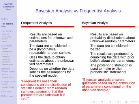
Bayesian Analysis vs Frequentist Analysis
Frequentist Analysis
• Results are based onestimations for unknown fixedparameters.
• The data are considered tobe a (hypothetical)repeatable random sample.
• Uses the data to obtainestimates about the unknownfixed parameters.
• Depends on whether the datasatisfies the assumptions forthe specified model.
"Frequentists base theirconclusions on the distribution ofstatistics derived from randomsamples, assuming that theparameters are unknown butfixed."
Bayesian Analyis
• Results are based onprobability distributions aboutunknown random parameters
• The data are considered tobe fixed.
• The results are produced bycombining the data with priorbeliefs about the parameters.
• The posterior distribution isused to make explicitprobabilistic statements
"Bayesian analysis answersquestions based on the distributionof parameters conditional on theobserved sample."
Bayesiananalysis in
Stata
Outline
The generalidea
The MethodBayes rule
Fundamentalequation
MCMC
Stata toolsbayesmh
bayesstats ess
Blocking
bayesgraph
bayes: prefix
bayesstats ic
bayestest model
RandomEffects ProbitThinning
bayestest interval
Change-pointmodelbayesgraph matrix
Summary
References
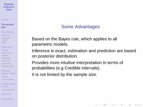
Some Advantages
• Based on the Bayes rule, which applies to allparametric models.
• Inference is exact, estimation and prediction are basedon posterior distribution.
• Provides more intuitive interpretation in terms ofprobabilities (e.g Credible intervals).
• It is not limited by the sample size.
Bayesiananalysis in
Stata
Outline
The generalidea
The MethodBayes rule
Fundamentalequation
MCMC
Stata toolsbayesmh
bayesstats ess
Blocking
bayesgraph
bayes: prefix
bayesstats ic
bayestest model
RandomEffects ProbitThinning
bayestest interval
Change-pointmodelbayesgraph matrix
Summary
References
Some Disadvantages
• Subjectivity in specifying prior beliefs.• Computationally challenging.• Setting up a model and performing analysis could be
an involving task.
Bayesiananalysis in
Stata
Outline
The generalidea
The MethodBayes rule
Fundamentalequation
MCMC
Stata toolsbayesmh
bayesstats ess
Blocking
bayesgraph
bayes: prefix
bayesstats ic
bayestest model
RandomEffects ProbitThinning
bayestest interval
Change-pointmodelbayesgraph matrix
Summary
References
Some Examples (Taken from Hahn, 2014)
• TranScan Medical use small dataset and priors basedon previous studies to determine the efficacy of its2000 device for mammografy (FDA 1999).
• homeprice.com.hk used Bayesian analysis for pricinginformation on over a million real state properties inHong Kong and surrounding areas (Shamdasany,2011).
• Researchers in the energy industry have usedBayesian analysis to understand petroleum reservoirparameters (Glinsky and Gunning, 2011).
Bayesiananalysis in
Stata
Outline
The generalidea
The MethodBayes rule
Fundamentalequation
MCMC
Stata toolsbayesmh
bayesstats ess
Blocking
bayesgraph
bayes: prefix
bayesstats ic
bayestest model
RandomEffects ProbitThinning
bayestest interval
Change-pointmodelbayesgraph matrix
Summary
References
The Method
• Let’s start by writing the Bayes’ Rule:
p (B|A) =p (A|B) p (B)
p (A)
Where:p (A|B): conditional probability of A given Bp (B|A): conditional probability of B given A
p (B): marginal probability of Bp (A): marginal probability of A
Bayesiananalysis in
Stata
Outline
The generalidea
The MethodBayes rule
Fundamentalequation
MCMC
Stata toolsbayesmh
bayesstats ess
Blocking
bayesgraph
bayes: prefix
bayesstats ic
bayestest model
RandomEffects ProbitThinning
bayestest interval
Change-pointmodelbayesgraph matrix
Summary
References
The Method
• If we have a probability model for a vector ofobservations y and a vector of unknown parameters θ,we can represent the model with a likelihood function:
L (θ; y) = f (y ; θ) =n∏
i=1
f (yi |θ)
Where:f (y ; θ): conditional probability of y give θ
• Let’s assume that θ has a probability distribution π (θ),and that denote m(y) denote the marginal distributionof y, such that:
m (y) =
∫f (y ; θ)π (θ) dθ
Bayesiananalysis in
Stata
Outline
The generalidea
The MethodBayes rule
Fundamentalequation
MCMC
Stata toolsbayesmh
bayesstats ess
Blocking
bayesgraph
bayes: prefix
bayesstats ic
bayestest model
RandomEffects ProbitThinning
bayestest interval
Change-pointmodelbayesgraph matrix
Summary
References
The Method
• Let’s now write the inverse law of probability (Bayes’Theorem):
f (θ|y) =f (y ; θ)π (θ)
f (y)
• But notice that the marginal distribution of y, f(y), doesnot depend on (θ)
• Then, we can write the fundamental equation forBayesian analysis:
p (θ|y) ∝ L (y |θ) π (θ)
Bayesiananalysis in
Stata
Outline
The generalidea
The MethodBayes rule
Fundamentalequation
MCMC
Stata toolsbayesmh
bayesstats ess
Blocking
bayesgraph
bayes: prefix
bayesstats ic
bayestest model
RandomEffects ProbitThinning
bayestest interval
Change-pointmodelbayesgraph matrix
Summary
References
Let’s go back to our initial example
Bayesiananalysis in
Stata
Outline
The generalidea
The MethodBayes rule
Fundamentalequation
MCMC
Stata toolsbayesmh
bayesstats ess
Blocking
bayesgraph
bayes: prefix
bayesstats ic
bayestest model
RandomEffects ProbitThinning
bayestest interval
Change-pointmodelbayesgraph matrix
Summary
References
The Method
• In the example we have the data (the likelihoodcomponent)
• We also have the experts belief (the prior component)• Then, how do we get the posterior distribution?• We use the fundamental equation
p (θ|y) ∝ L (y |θ)π (θ)
Bayesiananalysis in
Stata
Outline
The generalidea
The MethodBayes rule
Fundamentalequation
MCMC
Stata toolsbayesmh
bayesstats ess
Blocking
bayesgraph
bayes: prefix
bayesstats ic
bayestest model
RandomEffects ProbitThinning
bayestest interval
Change-pointmodelbayesgraph matrix
Summary
References
The Method• Let’s assume that both, the data and the prior beliefs,
are normally distributed:
• The data: y ∼ N(θ, σ2
d
)• The prior: θ ∼ N
(µp, σ
2p)
• Homework...: Doing the algebra with the fundamentalequation we find that the posterior distribution would benormal with:
• The posterior: θ|y ∼ N(µ, σ2
)Where:
µ = σ2 (Ny/σ2d + µp/σ
2p)
σ2 =(N/σ2
d + 1/σ2p)−1
Bayesiananalysis in
Stata
Outline
The generalidea
The MethodBayes rule
Fundamentalequation
MCMC
Stata toolsbayesmh
bayesstats ess
Blocking
bayesgraph
bayes: prefix
bayesstats ic
bayestest model
RandomEffects ProbitThinning
bayestest interval
Change-pointmodelbayesgraph matrix
Summary
References
The Method
• Doing the algebra was relatively straightforward in theprevious case.
• What about more complex distributions?• Integration is performed via simulation• We need to use intensive computational simulation
tools to find the posterior distribution in most cases.
• Markov chain Monte Carlo (MCMC) methods are thecurrent standard in most software. Stata implement twoalternatives:
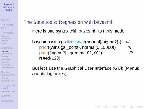
• But let’s use the Graphical User Interface (GUI) (Menusand dialog boxes):
Bayesiananalysis in
Stata
Outline
The generalidea
The MethodBayes rule
Fundamentalequation
MCMC
Stata toolsbayesmh
bayesstats ess
Blocking
bayesgraph
bayes: prefix
bayesstats ic
bayestest model
RandomEffects ProbitThinning
bayestest interval
Change-pointmodelbayesgraph matrix
Summary
References
The Stata tools: Menu for Bayesian regression
1 Make the following sequence of selection from the mainmenu:
Statistics > Bayesian analysis> General estimation and regression
2 Select ’Univariate linear models’3 Specify the dependent variable (wins) and the
explanatory variable (gs)
4 Select the ’Likelihood model’ (Normal regression)• For ’Variance’ click on ’Create’ and select ’Specify as a
model parameter’• Type ’sigma2’ in ’Parameter name’
Bayesiananalysis in
Stata
Outline
The generalidea
The MethodBayes rule
Fundamentalequation
MCMC
Stata toolsbayesmh
bayesstats ess
Blocking
bayesgraph
bayes: prefix
bayesstats ic
bayestest model
RandomEffects ProbitThinning
bayestest interval
Change-pointmodelbayesgraph matrix
Summary
References
The Stata tools: Menu for Bayesian regression
5 For "‘Priors of model parameters’ click on ’Create’• Select wins:gs and wins:_cons• Select the ’Normal distribution’• write ’0’ for the mean and ’10000’ for the variance.
6 Next, create the prior for the variance of the likelihoodsigma2
• Select the Inverse gamma distribution• Specify .01 and .01 for the ’Shape’ and ’Scale’
parameters.
7 Click on the ’Simulation’ tab and set the’Random-number seed’ to 123
1 Click on the ’Blocking’ tab2 Select ’Display block summary’3 Click on ’Create’4 Select wins:gs and wins:_cons and click ’OK’5 Click on ’Create’6 Select sigma2 and click ’OK’
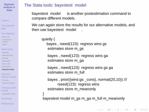
estimates store m_meanonly}bayestest model m_gs m_ga m_full m_meanonly
Bayesiananalysis in
Stata
Outline
The generalidea
The MethodBayes rule
Fundamentalequation
MCMC
Stata toolsbayesmh
bayesstats ess
Blocking
bayesgraph
bayes: prefix
bayesstats ic
bayestest model
RandomEffects ProbitThinning
bayestest interval
Change-pointmodelbayesgraph matrix
Summary
References
The Stata tools: bayestest model
• bayestest model computes the posterior probabilities foreach model.
• The result indicates which model is more likely.
• It requires that the models use the same data and that theyhave proper posterior.
• It can be used to compare models with:• Different priors and/or different posterior distributions.• Different regression functions.• Different covariates
• MCMC convergence should be verified before comparing themodels.
Bayesiananalysis in
Stata
Outline
The generalidea
The MethodBayes rule
Fundamentalequation
MCMC
Stata toolsbayesmh
bayesstats ess
Blocking
bayesgraph
bayes: prefix
bayesstats ic
bayestest model
RandomEffects ProbitThinning
bayestest interval
Change-pointmodelbayesgraph matrix
Summary
References
The Stata tools: bayestest model
• Here is the output for bayestest model
. bayestest model m_gs m_ga m_full m_meanonly
log(ML) P(M) P(M|y)
m_gs -135.7408 0.2500 0.8211
m_ga -148.5384 0.2500 0.0000
m_full -137.3534 0.2500 0.1637
m_meanonly -139.7326 0.2500 0.0152
Note: ML is computed using Laplace-Metropolis approximation.
• We could also assign different priors for the models:
. bayestest model m_gs m_ga m_full m_meanonly, ///
prior(.2 .1 .4 .3)
log(ML) P(M) P(M|y)
m_gs -135.7408 0.2000 0.7010
m_ga -148.5384 0.1000 0.0000
m_full -137.3534 0.4000 0.2795
m_meanonly -139.7326 0.3000 0.0194
Note: ML is computed using Laplace-Metropolis approximation.
Bayesiananalysis in
Stata
Outline
The generalidea
The MethodBayes rule
Fundamentalequation
MCMC
Stata toolsbayesmh
bayesstats ess
Blocking
bayesgraph
bayes: prefix
bayesstats ic
bayestest model
RandomEffects ProbitThinning
bayestest interval
Change-pointmodelbayesgraph matrix
Summary
References
Random Effects Probit model
Bayesiananalysis in
Stata
Outline
The generalidea
The MethodBayes rule
Fundamentalequation
MCMC
Stata toolsbayesmh
bayesstats ess
Blocking
bayesgraph
bayes: prefix
bayesstats ic
bayestest model
RandomEffects ProbitThinning
bayestest interval
Change-pointmodelbayesgraph matrix
Summary
References
The Stata tools: Random effects probit model
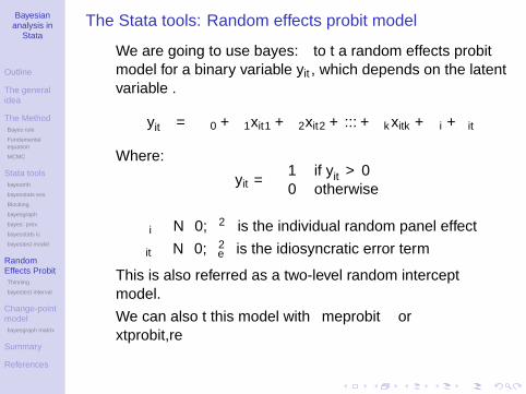
• We are going to use bayes: to fit a random effects probitmodel for a binary variable yit , which depends on the latentvariable .
• We check the scatterplots again for the simulated values ofthe coefficients and the variance.
. bayesgraph matrix
• We do not observe any pairwise correlations now.
Bayesiananalysis in
Stata
Outline
The generalidea
The MethodBayes rule
Fundamentalequation
MCMC
Stata toolsbayesmh
bayesstats ess
Blocking
bayesgraph
bayes: prefix
bayesstats ic
bayestest model
RandomEffects ProbitThinning
bayestest interval
Change-pointmodelbayesgraph matrix
Summary
References
The Stata tools: bayesgraph trace
• We can use bayesgraph trace to look at the trace for allthe parameters.
. bayesgraph trace
• The plots indicate that convergence seems to be achieved.
Bayesiananalysis in
Stata
Outline
The generalidea
The MethodBayes rule
Fundamentalequation
MCMC
Stata toolsbayesmh
bayesstats ess
Blocking
bayesgraph
bayes: prefix
bayesstats ic
bayestest model
RandomEffects ProbitThinning
bayestest interval
Change-pointmodelbayesgraph matrix
Summary
References
The Stata tools: bayesgraph ac
• We can also use bayesgraph ac to look at theautocorrelation for all the parameters.
. bayesgraph ac
• Autocorrelation decays and becomes negligible quickly foralmost all the parameters.
Bayesiananalysis in
Stata
Outline
The generalidea
The MethodBayes rule
Fundamentalequation
MCMC
Stata toolsbayesmh
bayesstats ess
Blocking
bayesgraph
bayes: prefix
bayesstats ic
bayestest model
RandomEffects ProbitThinning
bayestest interval
Change-pointmodelbayesgraph matrix
Summary
References
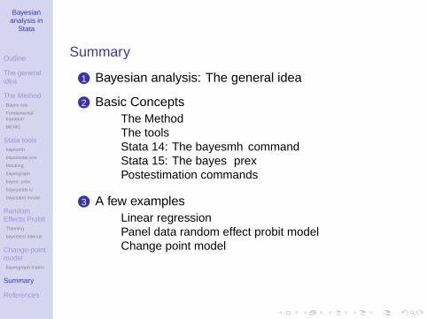
Summary
1 Bayesian analysis: The general idea
2 Basic Concepts• The Method• The tools• Stata 14: The bayesmh command• Stata 15: The bayes prefix• Postestimation commands
3 A few examples• Linear regression• Panel data random effect probit model• Change point model
Bayesiananalysis in
Stata
Outline
The generalidea
The MethodBayes rule
Fundamentalequation
MCMC
Stata toolsbayesmh
bayesstats ess
Blocking
bayesgraph
bayes: prefix
bayesstats ic
bayestest model
RandomEffects ProbitThinning
bayestest interval
Change-pointmodelbayesgraph matrix
Summary
References
References
Glinsky, M. E. and Gunnin, J. 2011. Understanding uncertainty in GSEM.World Oil, 232(1), 57—62, Jan. http://www.worldoil.com/Understanding-uncertainty-in-CSEM-January-2011.html,assessed-Jan.18,2012.
Hahn, Eugene D. 2014. Bayesian Methods for Management andBusiness: Pragmatic Solutions for Real Problems. John Wiley and Sons.
Shamdasany, P. 2011. Smart Money. South China Morning Post. p. 2.,Jul. 4.