Abstract We introduce the fundamental tenets of Bayesianinference, which derive from two basic laws of proba-bility theory. We cover the interpretation of probabilities,discrete and continuous versions of Bayes’ rule, parame-ter estimation, and model comparison. Using seven workedexamples, we illustrate these principles and set up some ofthe technical background for the rest of this special issue ofPsychonomic Bulletin & Review. Supplemental material isavailable via https://osf.io/wskex/.
Keywords Bayesian inference and parameter estimation ·Bayesian statistics · Tutorial
Dark and difficult times lie ahead. Soon we must allface the choice between what is right and what is easy.
A. P. W. B. Dumbledore
Introduction
Bayesian methods by themselves are neither dark nor, webelieve, particularly difficult. In some ways, however, theyare radically different from classical statistical methods andas such, rely on a slightly different way of thinking that mayappear unusual at first. Bayesian estimation of parameterswill usually not result in a single estimate, but will yielda range of estimates with varying plausibilities associatedwith them; and Bayesian hypothesis testing will rarely result
in the falsification of a theory but rather in a redistribu-tion of probability between competing accounts. Bayesianmethods are also not new, with their first use dating backto the 18th century. Nor are they new to psychology: Theywere introduced to the field over 50 years ago, in whattoday remains a remarkably insightful exposition by WardEdwards, Harold Lindman, and Savage (1963).
Nonetheless, until recently Bayesian methods have notbeen particularly mainstream in the social sciences, so therecent increase in their adoption means they are new tomost practitioners – and for many psychologists, learningabout new statistical techniques can evoke understandablefeelings of anxiety or trepidation. At the same time, recentrevelations regarding the reproducibility of psychologicalscience (e.g., Open Science Collaboration, 2015; Etz &Vandekerckhove, 2016) have spurred interest in the statisti-cal methods that find use in the field.
In the present article, we provide a gentle technical intro-duction to Bayesian inference (and set up the rest of thisspecial issue of Psychonomic Bulletin & Review), startingfrom first principles. We will first provide a short overviewinvolving the definition of probability, the basic laws ofprobability theory (the product and sum rules of probabil-ity), and how Bayes’ rule and its applications emerge fromthese two simple laws. We will then illustrate how the lawsof probability can and should be used for inference: to drawconclusions from observed data. We do not shy away fromshowing formulas and mathematical exposition, but wherepossible we connect them to a visual aid, either in a figure ora table, to make the concepts they represent more tangible.We also provide examples after each main section to illus-trate how these ideas can be put into practice. Most of thekey ideas outlined in this paper only require mathematicalcompetence at the level of college algebra; as will be seen,many of the formulas are obtained by rearranging equations
in creative ways such that the quantity of interest is on theleft-hand side of an equality.
At any point, readers more interested in the bigger pic-ture than the technical details can safely skip the equationsand focus on the examples and discussion. However, theuse of verbal explanations only suffices to gain a superfi-cial understanding of the underlying ideas and implications,so we provide mathematical formulas for those readers whoare interested in a deeper appreciation. Throughout the text,we occasionally use footnotes to provide extra notationalclarification for readers who may not be as well-versed withmathematical exposition.
While we maintain that the mathematical underpinningsserve understanding of these methods in important ways,we should also point out that recent developments regardingBayesian statistical software packages (e.g., Wagenmakers,Love, et al., this issue; Matzke, Boehm, & Vandekerckhove,this issue; van Ravenzwaaij, Cassey, & Brown, this issue;Wagenmakers, Marsman, et al., this issue) have made it pos-sible to perform many kinds of Bayesian analyses withoutthe need to carry out any of the technical mathemati-cal derivations. The mathematical basis we present hereremains, of course, more general.
First, however, we will take some time to discuss a subtlesemantic confusion between two interpretations of the keyconcept “probability.” The hurried reader may safely skipthe section that follows (and advance to “The Product andSum Rules of Probability”), knowing only that we use theword “probability” to mean “a degree of belief”: a quantitythat indicates how strongly we believe something to be true.
What is probability?
Throughout this text, we will be dealing with the conceptof probability. This presents an immediate philosophicalproblem, because the word “probability” is in some senseambiguous: it will occasionally switch from one meaningto another and this difference in meaning is sometimesconsequential.
In one meaning—sometimes called the epistemic1
interpretation—probability is a degree of belief : it is a num-ber between zero and one that quantifies how strongly weshould think something to be true based on the relevantinformation we have. In other words, probability is a math-ematical language for expressing our uncertainty. This kindof probability is inherently subjective—because it dependson the information that you have available—and reason-able people may reasonably differ in the probabilities thatthey assign to events (or propositions). Under the epis-temic interpretation, there is hence no such thing as theprobability—there is only your probability (Lindley, 2000).
1From Greek episteme, meaning knowledge.
Your probability can be thought of as characterizing yourstate of incomplete knowledge, and in that sense probabilitydoes not exist beyond your mind.
We may for example say “There is a 60% probability thatthe United Kingdom will be outside the European Union onDecember 31, 2018.” Someone who believes there is a 60%probability this event will occur should be willing to wagerup to $6 against $4 on the event, because their expectedgain would be at least 60% × (+4$) + 40% × (−6$),which is zero. In other words, betting more than $6 wouldbe unsound because they would expect to lose money, andto take such an action would not cohere with what theybelieve. Of course, in scientific practice one is rarely forcedto actually make such bets, but it would be unfortunate if ourprobabilities (and hence our inferences) could not be actedon with confidence if such an occasion were to arise (Hill,1974).
The fact that epistemic probabilities of events are sub-jective does not mean that they are arbitrary. Probabilitiesare not acts of will; they are subjective merely in the sensethat they may differ from one individual to the next. Thatis just to say that different people bring different informa-tion to a given problem.Moreover, if different people updatetheir beliefs in a rational way, then as data accumulate theywill gradually approach agreement (unless they have a pri-ori ruled out the point of agreement entirely; see, e.g., Jern,Chang, & Kemp, 2014). In fact, it can be shown that theonly way that our pre-data beliefs (whatever those may be)will cohere with our post-data beliefs is to use probability torepresent our uncertainty and update our beliefs accordingto the laws of probability (Lindley, 2000).
In another meaning—the physical or aleatory2
interpretation—probability is a statement of an expectedfrequency over many repetitions of a procedure. A state-ment of aleatory probability might be “If I flip a fair coinvery many times, the ratio of flips on which the coinwill come up heads is 50%. Thus, the probability that afair coin will come up heads is 50%.” These statementsexpress properties of the long-run behavior of well-definedprocesses, but they can not speak to singular events; theyrequire assumptions about physical repeatability and inde-pendence among repetitions. It is important to grasp thatthese frequencies are seen as being a real part of the phys-ical world, in that “the relative frequencies of a die fallingthis way or that way are ‘persistent’ and constitute thisdie’s measurable properties, comparable to its size andweight” (Neyman, 1977, p. 99). Neyman’s quote providesan interesting contrast to the epistemic interpretation. Ital-ian probabilist and influential Bayesian statistician Brunode Finetti famously began his treatise Theory of Proba-bility by stating “Probability does not exist” and that “the
2From Latin alea, meaning dice.
Psychon Bull Rev (2018) 25:5–34 7
abandonment of superstitious beliefs about the existence ofthe Phlogiston, the Cosmic Ether, Absolute Space and Time,. . . or Fairies and Witches was an essential step along theroad to scientific thinking. Probability, too, if regarded assomething endowed with some kind of objective existence,is no less a misleading misconception, an illusory attempt toexteriorize or materialize our true probabilistic beliefs” (DeFinetti, 1974, p. x). This is not to say that we cannot buildmodels that assign probabilities to the outcomes of physicalprocesses, only that they are necessarily abstractions.
It is clear that these two interpretations of probabilityare not the same. There are many situations to which thealeatory definition does not apply and thus probabilitiescould not be determined: we will not see repeated instancesof December 31, 2018, in which the UK could be inside oroutside the EU, we will only see one such event. Similarly,“what is the probability that this coin, on the very next flip,will come up heads?” is not something to which an aleatoryprobability applies: there are no long-run frequencies toconsider if there is only one flip that matters.
Aleatory probability may—in some cases—be a validconceptual interpretation of probability, but it is rarely everan operational interpretation (see Jaynes, 1984; Winkler,1972; Wrinch & Jeffreys, 1919): it cannot apply to singu-lar events such as the truth or falsity of a scientific theory,so we simply cannot speak of aleatory probabilities whenwrestling with the uncertainty we face in scientific prac-tice. That is to say, we may validly use aleatory probabilityto think about probability in an abstract way, but not tomake statements about real-world observed events such asexperimental outcomes.
In contrast, epistemic probability applies to any event thatwe care to consider—be it singular or repetitive—and if wehave relevant information about real-world frequencies thenwe can choose to use that information to inform our beliefs.If repetition is possible and we find it reasonable to assumethat the chance a coin comes up heads on a given toss doesnot change based on the outcome of previous tosses, thena Bayesian could reasonably believe both (a) that on thenext toss there is a 50% chance it comes up heads; and(b) 50% of tosses will result in heads in a very long seriesof flips. Hence, epistemic probability is both a conceptualinterpretation of probability and an operational interpreta-tion. Epistemic probability can be seen as an extension ofaleatory probability that applies to all the cases where thelatter would apply and to countless cases where it could not.
Why this matters We argue that the distinction aboveis directly relevant for empirical psychology. In the over-whelming majority of cases, psychologists are interestedin making probabilistic statements about singular events:this theory is either true or not; this effect is either pos-itive or negative; this effect size is probably between x
and y; and either this model or the other is more likelygiven the data. Seldom are we merely interested in the fre-quency with which a well-defined process will achieve acertain outcome. Even arbitrarily long sequences of faithfulreplications of empirical studies serve to address a singu-lar question: “is this theory correct?” We might reasonablydefine a certain behavioral model and assign parameters(even parameters that are probabilities) to it, and then exam-ine its long-run behavior. This is a valid aleatory question.However, it is not an inferential procedure: it describes thebehavior of an idealized model but does not provide us withinferences with regard to that model. We might also wonderhow frequently a researcher will make errors of inference(however defined) under certain conditions, but this is apurely academic exercise; unless the proportion of errors is0 or 1, such a long-run frequency alone does not allow usto determine the probability the researcher actually madean error regarding any singular finding—regarding thiscoin, this effect, or this hypothesis. By contrast, epistemicprobability expresses degrees of belief regarding specific,individual, singular events, and for that reason should be thedefault for scientific inference.
In the next section, we will introduce the basic rules ofprobability theory. These rules are agnostic to our concep-tion of probability—they hold equally for epistemic andaleatory probability—but throughout the rest of this paperand particularly in the examples, we will, unless other-wise noted, use an epistemic interpretation of the word“probability.”
The product and sum rules of probability
Here we will introduce the two cardinal rules of probabil-ity theory from which essentially all of Bayesian inferencederives. However, before we venture into the laws of prob-ability, there are notational conventions to draw. First, wewill use P(A) to denote the probability of some event A,where A is a statement that can be true or false (e.g., A
could be “it will rain today”, “the UK will be outside theEU on December 31, 2018”, or “the 20th digit of π is 3”).Next, we will use (B|A) to denote the conditional event:the probability that B is true given that A is true (e.g., B
could be “it will rain tomorrow”) is P(B|A): the probabilitythat it will rain tomorrow given that it rained today. Third,we will use (A, B) to denote a joint event: the probabilitythat A and B are both true is P(A,B). The joint probabilityP(A,B) is of course equal to that of the joint probabilityP(B,A): the event “it rains tomorrow and today” is logi-cally the same as “it rains today and tomorrow.” Finally, wewill use (¬A) to refer to the negation of A: the probabilityA is false is P(¬A). These notations can be combined: ifC and D represent the events “it is hurricane season” and“it rained yesterday,” respectively, then P(A,B|¬C,¬D) is
8 Psychon Bull Rev (2018) 25:5–34
the probability that it rains today and tomorrow, given that(¬C) it is not hurricane season and that (¬D) it did not rainyesterday (i.e., both C and D are not true).
With this notation in mind, we introduce the Product Ruleof Probability:
P(A,B) = P(B)P (A|B)
= P(A)P (B|A).(1)
In words: the probability that A and B are both true is equalto the probability of B multiplied by the conditional prob-ability of A assuming B is true. Due to symmetry, this isalso equal to the probability of A multiplied by the condi-tional probability of B assuming A is true. The probabilityit rains today and tomorrow is the probability it first rainstoday multiplied by the probability it rains tomorrow giventhat we know it rained today.
If we assume A and B are statistically independent thenP(B) equals P(B|A), since knowing A happens tells usnothing about the chance B happens. In such cases, theproduct rule simplifies as follows:
P(A,B) = P(A)P (B|A) = P(A)P (B). (2)
Keeping with our example, this would mean calculatingthe probability it rains both today and tomorrow in such away that knowledge of whether or not it rained today hasno bearing on how strongly we should believe it will raintomorrow.
Understanding the Sum Rule of Probability requires onefurther concept: the disjoint set. A disjoint set is nothingmore than a collection of mutually exclusive events. To sim-plify the exposition, we will also assume that exactly oneof these events must be true although that is not part of thecommon definition of such a set. The simplest example of adisjoint set is some event and its denial:3 {B, ¬B}. If B rep-resents the event “It will rain tomorrow,” then¬B representsthe event “It will not rain tomorrow.” One and only one ofthese events must occur, so together they form a disjoint set.If A represents the event “It will rain today,” and ¬A repre-sents “It will not rain today” (another disjoint set), then thereare four possible pairs of these events, one of which must betrue: (A, B), (A, ¬B), (¬A, B), and (¬A,¬B). The prob-ability of a single one of the singular events, say B, can befound by adding up the probabilities of all of the joint eventsthat contain B as follows:
P(B) = P(A,B) + P(¬A, B).
In words, the probability that it rains tomorrow is the sum oftwo joint probabilities: (1) the probability it rains today and
3We use curly braces {. . . } to indicate a set of events. Other com-mon examples of disjoint sets are the possible outcomes of a coin flip:{heads, tails}, or the possible outcomes of a roll of a six-sided die:{1, 2, 3, 4, 5, 6}. A particularly useful example is the truth of somemodelM, which must be either true or false: {M, ¬M}.
tomorrow, and (2) the probability it does not rain today butdoes rain tomorrow.
In general, if {A1, A2, . . . , AK} is a disjoint set, the SumRule of Probability states:
P(B) = P(A1, B) + P(A2, B) + . . . + P(AK, B)
=K∑
k=1
P(AK, B).(3)
That is, to find the probability of event B alone you addup all the joint probabilities that involve both B and oneelement of a disjoint set. Intuitively, it is clear that if oneof {A1, A2, . . . , AK} must be true, then the probability thatone of these and B is true is equal to the base probabilitythat B is true.
In the context of empirical data collection, the disjoint setof possible outcomes is often called the sample space.
An illustration of the Product Rule of Probability isshown by the path diagram in Fig. 1. Every fork indicatesthe start of a disjoint set, with each of the elements of that setrepresented by the branches extending out. The lines indi-cate the probability of selecting each element from withinthe set. Starting from the left, one can trace this diagram tofind the joint probability of, say, A and B. At the Start forkthere is a probability of .6 of going along the top arrow toevent A (a similar diagram could of course be drawn thatstarts with B): The probability it rains today is .6. Thenthere is a probability of .667 of going along the next top forkto event (A, B): The probability it rains tomorrow givenit rained today is .667. Hence, of the initial .6 probabilityassigned toA, two-thirds of it forks into (A, B), so the prob-ability of (A, B) is .6 × .667 = .40: Given that it rainedtoday, the probability it rains tomorrow is .667, so the proba-bility it rains both today and tomorrow is .4. The probabilityof any joint event at the end of a path can be found bymultiplying the probabilities of all the forks it takes to getthere.
Fig. 1 An illustration of the Product Rule of probability: The proba-bility of the joint events on the right end of the diagram is obtained bymultiplying the probabilities along the path that leads to it. The pathsindicate where and how we are progressively splitting the initial prob-ability into smaller subsets. A suggested exercise to test understandingand gain familiarity with the rules is to construct the equivalent pathdiagram (i.e., that in which the joint probabilities are identical) startingon the left with a fork that depends on the event B instead of A
Psychon Bull Rev (2018) 25:5–34 9
An illustration of the Sum Rule of Probability is shownin Table 1, which tabulates the probabilities of all the jointevents found through Fig. 1 in the main cells. For exam-ple, adding up all of the joint probabilities across the rowdenoted A gives P(A). Adding up all of the joint proba-bilities down the column denoted B gives P(B). This canalso be seen by noting that in Fig. 1, the probabilities ofthe two child forks leaving from A, namely (A, B) and(A, ¬B), add up to the probability indicated in the initialfork leading to A. This is true for any value of P(B|A) (andP(¬B|A) = 1 − P(B|A)).
What is Bayesian inference?
Together [the Sum and Product Rules] solve the prob-lem of inference, or, better, they provide a frameworkfor its solution.D. V. Lindley (2000)
Bayesian inference is the application of the product andsum rules to real problems of inference Applications ofBayesian inference are creative ways of looking at a prob-lem through the lens of these two rules. The rules form thebasis of a mature philosophy of scientific learning proposedby Dorothy Wrinch and Sir Harold Jeffreys (Jeffreys, 1961,1973; Wrinch and Jeffreys, 1921; see also Ly et al., 2016).Together, the two rules allow us to calculate probabilitiesand perform scientific inference in an incredible variety ofcircumstances. We begin by illustrating one combination ofthe two rules that is especially useful for scientific inference:Bayesian hypothesis testing.
Bayes’ Rule
Call event M (the truth of) an hypothesis that a researcherholds and call ¬M a competing hypothesis. Together thesecan form a disjoint set: {M, ¬M}. The set {M, ¬M} isnecessarily disjoint if ¬M is simply the denial of M, butin practice the set of hypotheses can contain any numberof models spanning a wide range of theoretical accounts.In such a scenario, it is important to keep in mind that
we cannot make inferential statements about any model notincluded in the set.
Before any data are collected, the researcher has somelevel of prior belief in these competing hypotheses, whichmanifest as prior probabilities and are denoted P(M) andP(¬M). The hypotheses are well-defined if they make aspecific prediction about the probability of each experimen-tal outcome X through the likelihood functions P(X|M)
and P(X|¬M). Likelihoods can be thought of as howstrongly the data X are implied by an hypothesis. Condi-tional on the truth of an hypothesis, likelihood functionsspecify the probability of a given outcome and are usuallyeasiest to interpret in relation to other hypotheses’ likeli-hoods. Of interest, of course, is the probability that M istrue, given the data X, or P(M|X).
By simple rearrangement of the factors of the Prod-uct Rule shown in the first line of Eq. 1, P(M, X) =P(X)P (M|X), we can derive that
P(M|X) = P(M, X)
P (X).
Due to the symmetric nature of the Product Rule, we canreformulate the joint event in the numerator above by apply-ing the product rule again as in the second line in Eq. 1,P(M, X) = P(M)P (X|M), and we see that this isequivalent to
P(M|X) = P(M)P (X|M)
P (X). (4)
Equation 4 is one common formulation of Bayes’ Rule,and analogous versions can be written for each of the othercompeting hypotheses; for example, Bayes’ Rule for¬M is
P(¬M|X) = P(¬M)P (X|¬M)
P (X).
The probability of an hypothesis given the data is equalto the probability of the hypothesis before seeing the data,multiplied by the probability that the data occur if thathypothesis is true, divided by the prior predictive probabil-ity of the observed data (see below). In the way that P(M)
and P(¬M) are called prior probabilities because they cap-ture our knowledge prior to seeing the data X, so P(M|X)
and P(¬M|X) are called the posterior probabilities.
Table 1 An illustration of the Sum Rule of Probability
B ¬B B or ¬B
A P(A, B) = .40 P(A, ¬B) = .20 ⇒ P(A) = .60
¬A P(¬A, B) = .15 P(¬A, ¬B) = .25 ⇒ P(¬A) = .40
A or ¬A P(B) = .55 P(¬B) = .45 1.00
The event A is that it rains today. The event B is that it rains tomorrow. Sum across rows to find P(A), sum down columns to find P(B). One canalso divide P(A,B) by P(A) to find P(B|A), as shown in the next section
10 Psychon Bull Rev (2018) 25:5–34
The prior predictive probability P(X)
Many of the quantities in Eq. 4 we know: we must havesome prior probability (belief or prior information) that thehypothesis is true if we are even considering the hypoth-esis at all, and if the hypothesis is well-described it willattach a particular probability to the observed data. Whatremains is the denominator: the prior predictive probabilityP(X)—the probability of observing a given outcome in theexperiment, which can be thought of as the average proba-bility of the outcome implied by the hypotheses, weightedby the prior probability of each hypothesis. P(X) can beobtained through the sum rule by adding the probabilities ofthe joint events P(X,M) and P(X, ¬M), as in Eq. 3, eachof which is obtained through an application of the productrule, so we obtain the following expression:
P(X) = P(X,M) + P(X, ¬M)
= P(M)P (X|M) + P(¬M)P (X|¬M),(5)
which amounts to adding up the right-hand side numera-tor of Bayes’ Rule for all competing hypotheses, giving aweighted-average probability of observing the outcome X.
Now that we have a way to compute P(X) in Eq. 5, wecan plug the result into the denominator of Eq. 4 as follows:
P(M|X) = P(M)P (X|M)
P (M)P (X|M) + P(¬M)P (X|¬M). (6)
Equation 6 is for the case where we are only consideringone hypothesis and its complement. More generally,
P(Mi |X) = P(Mi )P (X|Mi )∑Kk=1 P(Mk)P (X|Mk)
, (7)
for the case where we are considering K competing andmutually-exclusive hypotheses (i.e., hypotheses that form adisjoint set), one of which is Mi .
Quantifying evidence
Now that we have, in one equation, factors that correspondto our knowledge before—P(M)—and after—P(M|X)—seeing the data, we can address a slightly alternative ques-tion: How much did we learn due to the data X? Considerthat every quantity in Eq. 7 is either a prior belief in anhypothesis, or the probability that the data would occurunder a certain hypothesis—all known quantities. If wedivide both sides of Eq. 7 by P(Mi ),
P(Mi |X)
P (Mi )= P(X|Mi )∑K
k=1 P(Mk)P (X|Mk), (8)
we see that after observing outcome X, the ratio of anhypothesis’s posterior probability to its prior probability islarger than 1 (i.e., its probability goes up) if the probability it
attaches to the observed outcome is greater than a weighted-average of all such probabilities—averaged across all candi-date hypotheses, using the respective prior probabilities asweights.
If we are concerned with only two hypotheses, a par-ticularly interesting application of Bayes’ Rule becomespossible. After collecting data we are left with the posteriorprobability of two hypotheses, P(M|X) and P(¬M|X).If we form a ratio of these probabilities we can quantifyour relative belief in one hypothesis vis-a-vis the other, orwhat is known as the posterior odds: P(M|X)/P (¬M|X).If P(M|X) = .75 and P(¬M|X) = .25, the posteriorodds are .75/.25 = 3, or 3:1 (“three to one”) in favor of Mover ¬M. Since the posterior probability of an hypothesisis equal to the fraction in the right-hand side of Eq. 6, wecan calculate the posterior odds as a ratio of two right-handsides of Bayes’ Rule as follows:
P(M|X)
P (¬M|X)=
P(M)P (X|M)
P (M)P (X|M) + P(¬M)P (X|¬M)
P (¬M)P (X|¬M)
P (M)P (X|M) + P(¬M)P (X|¬M)
,
which can be reduced to a simple expression (since thedenominators cancel out),
P(M|X)
P (¬M|X)︸ ︷︷ ︸Posterior odds
= P(M)
P (¬M)︸ ︷︷ ︸Prior odds
× P(X|M)
P (X|¬M)︸ ︷︷ ︸Bayes factor
. (9)
The final factor—the Bayes factor—can be interpreted asthe extent to which the data sway our relative belief from onehypothesis to the other, which is determined by comparingthe hypotheses’ abilities to predict the observed data. If thedata are more probable under M than under ¬M (i.e., ifP(X|M) is larger than P(X|¬M)) thenM does the betterjob predicting the data, and the posterior odds will favorMmore strongly than the prior odds.
It is important to distinguish Bayes factors from posteriorprobabilities. Both are useful in their own role—posteriorprobabilities to determine our total belief after taking intoaccount the data and to draw conclusions, and Bayes fac-tors as a learning factor that tells us how much evidencethe data have delivered. It is often the case that a Bayesfactor favors M over ¬M while at the same time theposterior probability of ¬M remains greater than M. AsJeffreys, in his seminal paper introducing the Bayes factoras a method of inference, explains: “If . . . the [effect] exam-ined is one that previous considerations make unlikely toexist, then we are entitled to ask for a greater increase ofthe probability before we accept it,” and moreover, “To raisethe probability of a proposition from 0.01 to 0.1 does notmake it the most likely alternative” (Jeffreys, 1935, p. 221).This distinction is especially relevant to today’s publish-ing environment, where there exists an incentive to publish
Psychon Bull Rev (2018) 25:5–34 11
counterintuitive results—whose very description as counter-intuitive implies most researchers would not have expectedthem to be true. Consider as an extreme example (Bem,2011) who presented data consistent with the hypothesisthat some humans can predict future random events. WhileBem’s data may indeed provide positive evidence for thathypothesis (Rouder and Morey, 2011), it is staggeringlyimprobable a priori and the evidence in the data does notstack up to the strong priors many of us will have regard-ing extrasensory perception—extraordinary claims requireextraordinary evidence.
Since Bayes factors quantify statistical evidence, theycan serve two (closely related) purposes. First, evidence canbe applied to defeat prior odds: supposing that prior to thedata we believe that ¬M is three times more likely thanM(i.e., the prior ratio favoring ¬M is 3, or its prior proba-bility is 75%), we need a Bayes factor favoring M that isgreater than 3 so thatMwill end up the more likely hypoth-esis. Second, evidence can be applied to achieve a desiredlevel of certainty: supposing that we desire a high degree ofcertainty before making any practical decision (say, at least95% certainty or a posterior ratio of at least 19) and suppos-ing the same prior ratio as before, then we would require aBayes factor of 19 × 3 = 57 to defeat the prior odds andobtain this high degree of certainty. These practical consid-erations (often left implicit) are formalized by utility (loss)functions in Bayesian decision theory. We will not go intoBayesian decision theory in depth here; introductions can befound in Lindley (1985) or Winkler (1972), and an advancedintroduction is available in Robert (2007).
In this section, we have derived Bayes’ Rule as a neces-sary consequence of the laws of probability. The rule allowsus to update our belief regarding an hypothesis in responseto data. Our beliefs after taking account the data are capturedin the posterior probability, and the amount of updating isgiven by the Bayes factor. We now move to some appliedexamples that illustrate how this simple rule pertains tocases of inference.
Example 1: “The happy herbologist” At HogwartsSchool of Witchcraft and Wizardry,4 professor PomonaSprout leads the Herbology Department (see Illustration).In the Department’s greenhouses, she cultivates crops of amagical plant called green codacle—a flowering plant thatwhen consumed causes a witch or wizard to feel euphoricand relaxed. Professor Sybill Trelawney, the professor ofDivination, is an avid user of green codacle and frequentlyvisits Professor Sprout’s laboratory to sample the latestharvest.
However, it has turned out that one in a thousand codacleplants is afflicted with a mutation that changes its effects:
Consuming those rare plants causes unpleasant side effectssuch as paranoia, anxiety, and spontaneous levitation. Inorder to evaluate the quality of her crops, Professor Sprouthas developed a mutation-detecting spell. The new spell hasa 99% chance to accurately detect an existing mutation, butalso has a 2% chance to falsely indicate that a healthy plantis a mutant. When Professor Sprout presents her results at aSchool colloquium, Trelawney asks two questions: What isthe probability that a codacle plant is a mutant, when yourspell says that it is? And what is the probability the plant is amutant, when your spell says that it is healthy? Trelawney’sinterest is in knowing how much trust to put into ProfessorSprout’s spell.
Call the event that a specific plant is a mutant M, andthat it is healthy ¬M. Call the event that Professor Sprout’sspell diagnoses a plant as a mutant D, and that it diag-noses it healthy ¬D. Professor Trelawney’s interest is inthe probability that the plant is indeed a mutant given thatit has been diagnosed as a mutant, or P(M|D), and theprobability the plant is a mutant given it has been diag-nosed healthy, or P(M|¬D). Professor Trelawney, who isan accomplished statistician, has all the relevant informationto apply Bayes’ Rule (Eq. (7) above) to find these prob-abilities. She knows the prior probability that a plant is amutant is P(M) = .001, and thus the prior probability thata plant is not a mutant is P(¬M) = 1 − P(M) = .999.The probability of a correct mutant diagnosis given the plantis a mutant is P(D|M) = .99, and the probability of anerroneous healthy diagnosis given the plant is a mutant is
12 Psychon Bull Rev (2018) 25:5–34
thus P(¬D|M) = 1 − P(D|M) = .01. When the plantis healthy, the spell incorrectly diagnoses it as a mutantwith probability P(D|¬M) = .02, and correctly diag-noses the plant as healthy with probability P(¬D|¬M) =1 − P(D|¬M) = .98.
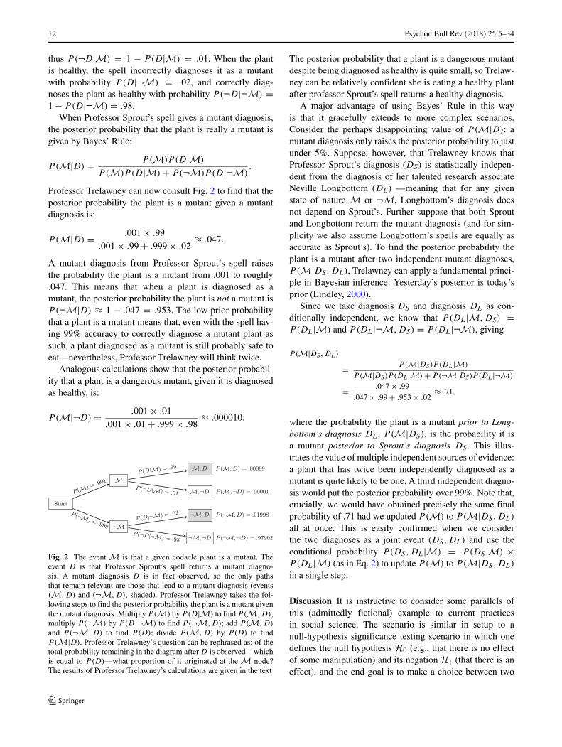
When Professor Sprout’s spell gives a mutant diagnosis,the posterior probability that the plant is really a mutant isgiven by Bayes’ Rule:
P(M|D) = P(M)P (D|M)
P (M)P (D|M) + P(¬M)P (D|¬M).
Professor Trelawney can now consult Fig. 2 to find that theposterior probability the plant is a mutant given a mutantdiagnosis is:
P(M|D) = .001 × .99
.001 × .99 + .999 × .02≈ .047.
A mutant diagnosis from Professor Sprout’s spell raisesthe probability the plant is a mutant from .001 to roughly.047. This means that when a plant is diagnosed as amutant, the posterior probability the plant is not a mutant isP(¬M|D) ≈ 1 − .047 = .953. The low prior probabilitythat a plant is a mutant means that, even with the spell hav-ing 99% accuracy to correctly diagnose a mutant plant assuch, a plant diagnosed as a mutant is still probably safe toeat—nevertheless, Professor Trelawney will think twice.
Analogous calculations show that the posterior probabil-ity that a plant is a dangerous mutant, given it is diagnosedas healthy, is:
P(M|¬D) = .001 × .01
.001 × .01 + .999 × .98≈ .000010.
Fig. 2 The event M is that a given codacle plant is a mutant. Theevent D is that Professor Sprout’s spell returns a mutant diagno-sis. A mutant diagnosis D is in fact observed, so the only pathsthat remain relevant are those that lead to a mutant diagnosis (events(M, D) and (¬M, D), shaded). Professor Trelawney takes the fol-lowing steps to find the posterior probability the plant is a mutant giventhe mutant diagnosis: Multiply P(M) by P(D|M) to find P(M, D);multiply P(¬M) by P(D|¬M) to find P(¬M, D); add P(M, D)
and P(¬M, D) to find P(D); divide P(M, D) by P(D) to findP(M|D). Professor Trelawney’s question can be rephrased as: of thetotal probability remaining in the diagram after D is observed—whichis equal to P(D)—what proportion of it originated at the M node?The results of Professor Trelawney’s calculations are given in the text
The posterior probability that a plant is a dangerous mutantdespite being diagnosed as healthy is quite small, so Trelaw-ney can be relatively confident she is eating a healthy plantafter professor Sprout’s spell returns a healthy diagnosis.
A major advantage of using Bayes’ Rule in this wayis that it gracefully extends to more complex scenarios.Consider the perhaps disappointing value of P(M|D): amutant diagnosis only raises the posterior probability to justunder 5%. Suppose, however, that Trelawney knows thatProfessor Sprout’s diagnosis (DS) is statistically indepen-dent from the diagnosis of her talented research associateNeville Longbottom (DL) —meaning that for any givenstate of nature M or ¬M, Longbottom’s diagnosis doesnot depend on Sprout’s. Further suppose that both Sproutand Longbottom return the mutant diagnosis (and for sim-plicity we also assume Longbottom’s spells are equally asaccurate as Sprout’s). To find the posterior probability theplant is a mutant after two independent mutant diagnoses,P(M|DS, DL), Trelawney can apply a fundamental princi-ple in Bayesian inference: Yesterday’s posterior is today’sprior (Lindley, 2000).
Since we take diagnosis DS and diagnosis DL as con-ditionally independent, we know that P(DL|M, DS) =P(DL|M) and P(DL|¬M, DS) = P(DL|¬M), giving
P(M|DS, DL)
= P(M|DS)P (DL|M)
P (M|DS)P (DL|M) + P(¬M|DS)P (DL|¬M)
= .047 × .99
.047 × .99 + .953 × .02≈ .71,
where the probability the plant is a mutant prior to Long-bottom’s diagnosis DL, P(M|DS), is the probability it isa mutant posterior to Sprout’s diagnosis DS . This illus-trates the value of multiple independent sources of evidence:a plant that has twice been independently diagnosed as amutant is quite likely to be one. A third independent diagno-sis would put the posterior probability over 99%. Note that,crucially, we would have obtained precisely the same finalprobability of .71 had we updated P(M) to P(M|DS, DL)
all at once. This is easily confirmed when we considerthe two diagnoses as a joint event (DS, DL) and use theconditional probability P(DS, DL|M) = P(DS |M) ×P(DL|M) (as in Eq. 2) to update P(M) to P(M|DS, DL)
in a single step.
Discussion It is instructive to consider some parallels ofthis (admittedly fictional) example to current practicesin social science. The scenario is similar in setup to anull-hypothesis significance testing scenario in which onedefines the null hypothesis H0 (e.g., that there is no effectof some manipulation) and its negation H1 (that there is aneffect), and the end goal is to make a choice between two
Psychon Bull Rev (2018) 25:5–34 13
possible decisions {D,¬D};D means deciding to rejectH0,and ¬D means deciding not to reject H0. In the exampleabove the rate at which we falsely reject the null hypothe-sis (i.e., deciding to reject it when in fact it is true) is givenby P(D|¬M) = .02—this is what is commonly called thefalse alarm rate. The rate at which we correctly reject thenull hypothesis (i.e., rejecting it if it is false) is P(D|M) =.99. However, even with a low false alarm rate and a veryhigh correct rejection rate, a null hypothesis rejection maynot necessarily provide enough evidence to overcome thelow prior probability an alternative hypothesis might have.
Example 2: “A curse on your hat” At the start of everyschool year, new Hogwarts students participate in thecenturies-old Sorting ceremony, during which they areassigned to one of the four Houses of the School:Gryffindor, Hufflepuff, Ravenclaw, or Slytherin. Theassignment is performed by the Sorting Hat, a pointy hatwhich, when placed on a student’s head, analyzes their abil-ities and personality before loudly calling out the House thatit determines as the best fit for the student. For hundreds ofyears the Sorting Hat has assigned students to houses withperfect accuracy and in perfect balance (one-quarter to eachHouse).
Unfortunately, the Hat was damaged by a stray curse dur-ing a violent episode at the School. As a result of the darkspell, the Hat will now occasionally blurt out “Slytherin!”even when the student’s proper alliance is elsewhere. Now,the Hat places exactly 40% of first-years in Slytherin insteadof the usual 25%, and each of the other Houses get only 20%of the cohort.
To attempt to correct the House assignment, ProfessorCuthbert Binns has developed a written test—the Place-ment Accuracy Remedy for Students Erroneously Labeledor P.A.R.S.E.L. test—on which true Slytherins will tendto score Excellent (SE), while Ravenclaws will tend toscore Outstanding (SO ), Gryffindors Acceptable (SA), andHufflepuffs Poor (SP ). Benchmark tests on students whowere Sorted before the Hat was damaged have revealed theapproximate distribution of P.A.R.S.E.L. scores within eachHouse (see Table 2). The test is administered to all studentswho are sorted into Slytherin House by the damaged Sort-ing Hat, and their score determines the House to which theyare assigned. Headmistress Minerva McGonagall, who isa Gryffindor, asks Professor Binns to determine the prob-ability that a student who was sorted into Slytherin andscored Excellent on the P.A.R.S.E.L. test actually belongs inGryffindor.
The solution relies on the repeated and judicious appli-cation of the Sum and Product Rules, until an expressionappears with the desired quantity on the left-hand side andonly known quantities on the right-hand side. To begin, Pro-fessor Binns writes down Bayes’ Rule (remembering that
Table 2 Probability of each P.A.R.S.E.L. score by true Houseaffiliation
Excellent(SE)
Outstanding(SO )
Acceptable(SA)
Poor(SP )
Slytherin (MS ) 0.80 0.10 0.05 0.05
Gryffindor (MG) 0.05 0.20 0.70 0.05
Ravenclaw (MR) 0.05 0.80 0.15 0.00
Hufflepuff (MH ) 0.00 0.10 0.25 0.65
Each value indicates the conditional probability P(S|M), that is, theprobability that a student from houseM obtains score S
a joint event like (DS, SE) can be treated like any otherevent):
P(MG|DS, SE) = P(MG)P (DS, SE |MG)
P (DS, SE)
Here, MG means that the true House assignment isGryffindor, DS means that the Sorting Hat placed them inSlytherin, and SE means the student scored Excellent on theP.A.R.S.E.L. test.
In most simple cases, we often have knowledge of sim-ple probabilities, of the form P(A) and P(B|A), while theprobabilities of joint events (A, B) are harder to obtain. ForProfessor Binns’ problem, we can overcome this difficultyby using the Product Rule to unpack the joint event in thenumerator:5
P(MG|DS, SE) = P(MG)P (SE |MG)P (DS |SE,MG)
P (DS, SE).
Now we discover the probability P(DS |SE,MG) in thenumerator. Since the cursed hat’s recommendation does notadd any information about the P.A.R.S.E.L. score aboveand beyond the student’s true House affiliation (i.e., it isconditionally independent; the test score is not entirelyindependent of the hat’s recommendation since the hat isoften right about the student’s correct affiliation and theaffiliation influences the test score), we can simplify thisconditional probability: P(DS |SE,MG) = P(DS |MG).Note that the numerator now only contains known quan-tities: P(SE |MG) can be read off as 0.05 from Table 2;P(DS |MG) is the probability that a true Gryffindor is erro-neously sorted into Slytherin, and since that happens to onein five true Gryffindors (because the proportion sorted intoGryffindor went down from 25 to 20%), P(DS |MG) must
5Note that this is an application of the Product Rule to the sce-nario where both events are conditional on MG: P(DS, SE |MG) =P(SE |MG)P (DS |SE,MG).
14 Psychon Bull Rev (2018) 25:5–34
be 0.20; and P(MG) is the base probability that a studentis a Gryffindor, which we know to be one in four. Thus,
P(MG|DS, SE) = P(MG)P (SE |MG)P (DS |MG)
P (DS, SE)
= 0.25 × 0.05 × 0.20
P(DS, SE).
This leaves us having to find P(DS, SE), the prior predic-tive probability that a student would be Sorted into Slytherinand score Excellent on the P.A.R.S.E.L. test. Here, the SumRulewill help us out, because we can find the right-hand sidenumerator for each type of student in the same way we didfor true Gryffindors above—we can find P(DS, SE |Mi ) forany House i = S, G, R, H . Hence (from Eq. 3),
P(DS, SE) =∑
i
P (Mi )P (SE |Mi )P (DS |Mi )
= P(MS)P (SE |MS)P (DS |MS)
+ P(MG)P (SE |MG)P (DS |MG)
+ P(MR)P (SE |MR)P (DS |MR)
+ P(MH )P (SE |MH )P (DS |MH )
= 0.25 × 0.80 × 1.00
+ 0.25 × 0.05 × 0.20
+ 0.25 × 0.05 × 0.20
+ 0.25 × 0.00 × 0.20
= 0.2050.
So finally, we arrive at:
P(MG|DS, SE) = 0.0025
0.2050= 0.0122,
which allows Professor Binns to return to the Headmistresswith good news: There is only around a 1% probabil-ity that a student who is Sorted into Slytherin and scoresExcellent on the P.A.R.S.E.L. test is actually a Gryffindor.Furthermore, Binns claims that the probability that sucha student is a true Slytherin is over 95%, and that thecombined procedure—that consists of first letting the Sort-ing Hat judge and then giving Slytherin-placed studentsa P.A.R.S.E.L. test and rehousing them by their score—will correctly place students of any House with at least90% probability. For example, he explains, a true Raven-claw would be sorted into their correct House by the Hatwith 80% (P(DR|MR)) probability, and would be placedinto Slytherin with 20% probability. In the second case,the student would be given the P.A.R.S.E.L. test, in whichthey would obtain an Outstanding with 80% (P(SO |MR))probability. Hence, they would be placed in their cor-rect House with probability P(DR|MR) + P(DS |MR) ×P(SO |MR) = 0.80 + 0.20 × 0.80 = 0.96.
Discussion The Sorting Hat example introduces two exten-sions from the first. Here, there are not two but four
possible “models”—whereas statistical inference is often seenas a choice problem between two alternatives, probabilis-tic inference naturally extends to any number of alternativehypotheses. The extension that allows for the evaluation ofmultiple hypotheses did not require the ad hoc formulationof any new rules, but relied entirely on the same basic rulesof probability.
The example additionally underscores an inferentialfacility that we believe is vastly underused in social science:we selected between models making use of two qualitativelydifferent sources of information. The two sources of infor-mation were individually insufficient but jointly powerful:the Hat placement is only 80% accurate in most cases, andthe written test was only 50% accurate for the Ravenclawcase, but together they are 90% accurate. Again, this exten-sion is novel only in that we had not yet considered it – thefact that information from multiple sources can be so com-bined requires no new facts and is merely a consequence ofthe two fundamental rules of probability.
Probability theory in the continuous case
In Bayesian parameter estimation, both the prior andposterior distributions represent, not any measurableproperty of the parameter, but only our own state ofknowledge about it. The width of the [posterior] dis-tribution. . . indicates the range of values that are con-sistent with our prior information and data, and whichhonesty therefore compels us to admit as possible values.E. T. Jaynes (1986)
The full power of probabilistic inference will come tolight when we generalize from discrete events A with prob-abilities P(A), to continuous parameters a with probabilitydensities p(a).6 Probability densities are different fromprobabilities in many ways. Densities express how muchprobability exists “near” a particular value of a, while theprobability of any particular value of a in a continuous rangeis zero. Probability densities cannot be negative but they canbe larger than 1, and they translate to probabilities throughthe mathematical operation of integration (i.e., calculatingthe area under a function over a certain interval). Possiblythe most well-known distribution in psychology is the theo-retical distribution of IQ in the population, which is shownin Fig. 3.
By definition, the total area under a probability densityfunction is 1:
1 =∫
A
p(a)da,
6When we say a parameter is “continuous” we mean it could take anyone of the infinite number of values comprising some continuum. Forexample, this would apply to values that follow a normal distribution.
Psychon Bull Rev (2018) 25:5–34 15
0.00
0.01
0.02
0.03
50 75 100 125 150
Fig. 3 An example of a probability density function (PDF). PDFsexpress the relative plausibility of different values and can be used todetermine the probability that a value lies in any interval. The PDFshown here is the theoretical distribution of IQ in the population: anormal distribution (a.k.a. Gaussian distribution) with mean 100 andstandard deviation 15. In this distribution, the filled region to the leftof 81 has an area of approximately 0.10, indicating that for a randommember of the population, there is a 10% chance their IQ is below 81.Similarly, the narrow shaded region on the right extends from 108 to113 and also has an area of 0.10, meaning that a random member hasa 10% probability of falling in that region
where capitalized A indicates that the integration is over theentire range of possible values for the parameter that appearsat the end—in this case a. The range A is hence a disjointset of possible values for a. For instance, if a is the mean ofa normal distribution, A indicates the range of real numbersfrom −∞ to ∞; if a is the rate parameter for a binomialdistribution, A indicates the range of real numbers between0 and 1. The symbol da is called the differential and thefunction that appears between the integration sign and thedifferential is called the integrand—in this case p(a).
We can consider how much probability is containedwithin smaller sets of values within the range A; for exam-ple, when dealing with IQ in the population, we couldconsider the integral over only the values of a that are lessthan 81, which would equal the probability that a is less than81:7
P(a < 81) =∫ 81
−∞p(a)da.
In Fig. 3, the shaded area on the left indicates the probabilitydensity over the region (−∞, 81).
The fundamental rules of probability theory in the dis-crete case—the sum and product rules—have continuousanalogues. The continuous form of the product rule is
7Strictly speaking, this integral is the probability that a is less thanor equal to 81, but the probability of any single point in a continuousdistribution is 0. By the sum rule, P(a ≤ 81) = P(a < 81) + P(a =81), which simplifies to P(a ≤ 81) = P(a < 81) + 0.
essentially the same as in the discrete case: p(a, b) =p(a)p(b|a), where p(a) is the density of the continuousparameter a and p(b|a) denotes the conditional density ofb (i.e., the density of b assuming a particular value of a).As in the discrete case of Eq. 1, it is true that p(a, b) =p(a)p(b|a) = p(b)p(a|b), and that p(a, b) = p(a)p(b) ifwe consider a and b to be statistically independent. For thecontinuous sum rule, the summation in Eq. 3 is replaced byan integration over the entire parameter space B:
p(a) =∫
B
p(a, b)db.
Because this operation can be visualized as a function overtwo dimensions (p(a, b) is a function that varies over a
and b simultaneously) that is being collapsed into the one-dimensional margin (p(a) varies only over a), this operationis alternatively calledmarginalization, integrating over b, orintegrating out b.
Using these continuous forms of the sum and productrules, we can derive a continuous form of Bayes’ Rule bysuccessively applying the continuous sum and product rulesto the numerator and denominator (analogously to Eq. 7):
p(a|b) = p(a, b)
p(b)= p(a)p(b|a)
p(b)
= p(a)p(b|a)∫A
p(a)p(b|a)da.
(10)
Since the product in the numerator is divided by its ownintegral, the total area under the posterior distributionalways equals 1; this guarantees that the posterior is alwaysa proper distribution if the prior and likelihood are properdistributions. It should be noted that by “continuous formof Bayes’ Rule” we mean that the prior and posterior dis-tributions for the model parameter(s) are continuous—thesample data can still be discrete, as in Example 3 below.
One application of Bayesian methods to continuousparameters is estimation. If θ (theta) is a parameter of inter-est (say, the success probability of a participant in a task),then information about the relative plausibility of differentvalues of θ is given by the probability density p(θ). If newinformation becomes available, for example in the form ofnew data x, the density can be updated and made conditionalon x:
p(θ |x) = p(θ)p(x|θ)
p(x)= p(θ)p(x|θ)∫
�p(θ)p(x|θ)dθ
. (11)
Since in the context of scientific learning these two den-sities typically represent our knowledge of a parameter θ
before and after taking into account the new data x, p(θ) isoften called the prior density and p(θ |x) the posterior den-sity. Obtaining the posterior density involves the evaluation
16 Psychon Bull Rev (2018) 25:5–34
of Eq. 11 and requires one to define a likelihood functionp(x|θ), which indicates how strongly the data x are impliedby every possible value of the parameter θ .
The numerator on the right-hand side of Eq. 11,p(θ)p(x|θ), is a product of the prior distribution and thelikelihood function, and it completely determines the shapeof the posterior distribution (note that the denominator inthat equation is not a function of the parameter θ ; eventhough the parameter seems to feature in the integrand, itis in fact “integrated out” so that the denominator dependsonly on the data x). For this reason, many authors pre-fer to ignore the denominator of Eq. 11 and simply writethe posterior density as proportional to the numerator, asin p(θ |x) ∝ p(θ)p(x|θ). We do not, because this con-ceals the critical role the denominator plays in a predictiveinterpretation of Bayesian inference.
The denominator p(x) is the weighted-average proba-bility density of the data x, where the form of the priordistribution determines the weights. This normalizing con-stant is the continuous analogue of the prior predictivedistribution, often alternatively referred to as the marginallikelihood or the Bayesian evidence.8 Consider that, in asimilar fashion to the discrete case, we can rearrange Eq. 11as follows—dividing each side by p(θ)—to illuminate inan alternative way how Bayes’ rule operates in updat-ing the prior distribution p(θ) to a posterior distributionp(θ |x):
p(θ |x)
p(θ)= p(x|θ)
p(x)= p(x|θ)∫
�p(θ)p(x|θ)dθ
. (12)
On the left-hand side, we see the ratio of the posterior tothe prior density. Effectively, this tells us for each value ofθ how much more or less plausible that value became dueto seeing the data x. The equation shows that this ratio isdetermined by how well that specific value of θ predictedthe data, in comparison to the weighted-average predictiveaccuracy across all values in the range �. In other words,parameter values that exceed the average predictive accu-racy across all values in � have their densities increased,while parameter values that predict worse than the aver-age have their densities decreased (see Morey, Romeijn, &Rouder, 2016; Wagenmakers, Morey, & Lee, in press).
While the discrete form of Bayes’ rule has natural appli-cations in hypothesis testing, the continuous form morenaturally lends itself to parameter estimation. Examples ofsuch questions are: “What is the probability that the regres-sion weight β is positive?” and “What is the probabilitythat the difference between these means is between δ =−.3 and δ = .3?” These questions can be addressed in a
8We particularly like Evans’s take on the term Bayesian evidence: “Forevidence, as expressed by observed data in statistical problems, is whatcauses beliefs to change and so we can measure evidence by measuringchange in belief” (Evans, 2014, p. 243).
straightforward way, using only the product and sum rulesof probability.
Example 3: “Perfection of the puking pastille” In thesecretive research and development laboratory of Weasley’sWizarding Wheezes, George Weasley works to develop gagtoys and prank foods for the entertainment of young witchesand wizards. In a recent project, Weasley is studying theeffects of his store’s famous puking pastilles, which causeimmediate vomiting when consumed. The target audienceis Hogwarts students who need an excuse to leave class andenjoy making terrible messes.
Shortly after the pastilles hit Weasley’s store shelves,customers began to report that puking pastilles cause notone, but multiple “expulsion events.” To learn more aboutthis unknown behavior, George turns to his sister Ginnyand together they decide to set up an exploratory study.From scattered customer reports, George believes the expul-sion rate to be between three to five events per hour, buthe intends to collect data to determine the rate more pre-cisely. At the start of this project, George has no distincthypotheses to compare—he is interested only in estimatingthe expulsion rate.
Since the data x are counts of the number of expulsionevents within an interval of time, Ginny decides that theappropriate model for the data (i.e., likelihood function) is aPoisson distribution (see top panel of Fig. 4):
p(x|λ) = 1
x! exp (−λ) λx, (13)
with the λ (lambda) parameter representing the expectednumber of events within the time interval (note exp(−λ) issimply a clearer way to write e−λ).
A useful prior distribution for Poisson rates is the Gammadistribution (Gelman et al., 2004, Appendix A):9
p(λ|a, b) = ba
�(a)exp (−λb) λa−1, (14)
A visual representation of the Gamma distribution is givenin the second panel of Fig. 4. A Gamma distribution has twoparameters that determine its form, namely shape (a) andscale (b).10 The Gamma distribution is useful here for two
9Recall that x! = x×(x−1)×· · ·×1 (where x! is read as “the factorialof x,” or simply “x factorial”). Similarly, the Gamma function �(a) isequal to (a − 1)! = (a − 1) × (a − 2) × · · · × 1 when a is an integer.Unlike a factorial, however, the Gamma function is more flexible inthat it can be applied to non-integers.10To ease readability we use Greek letters for the parameters of a likeli-hood function and Roman letters for the parameters of prior (posterior)distributions. The parameters that characterize a distribution can befound on the right side of the conditional bar; for instance, the likeli-hood function p(x|λ) has parameter λ, whereas the prior distributionp(λ|a, b) has parameters (a, b).
Fig. 4 Top row:An example Poisson distribution. The function is p(x|λ = 7) as defined in Eq. 13. The height of each bar indicates the probabilityof that particular outcome (e.g., number of expulsion events). Second row: The prior distribution of λ; a Gamma distribution with parametersa = 2 and b = 0.2. This is the initial state of the Weasley’s knowledge of the expulsion rate λ (the expected number of expulsion events per hour).Third row: The likelihood functions associated with x1 = 7 (left), x2 = 8 (center), and x3 = 19 (right). Bottom row: The posterior distribution ofλ; a Gamma distribution with parameters a = 36 and b = 3.2. This is the final state of knowledge regarding λ
reasons: first, it has the right support, meaning that it pro-vides nonzero density for all possible values for the rate (inthis case all positive real numbers); and second, it is conju-gate with the Poisson distribution, a technical property to beexplained below.
Before collecting further data, the Weasleys make sure tospecify what they believe to be reasonable values based onthe reports George has heard. In the second panel of Fig. 4,Ginny set the prior parameters to a = 2 and b = 0.2 bydrawing the shape of the distribution for many parametercombinations and selecting a curve that closely resemblesGeorge’s prior information: Values between three and fiveare most likely, but the true value of the expulsion rate couldconceivably be much higher.
Three volunteers are easily found, administered one puk-ing pastille each, and monitored for 1 h. The observed eventfrequencies are x1 = 7, x2 = 8, and x3 = 19.
With the prior density (14) and the likelihood (13)known, Ginny can use Bayes’ rule as in Eq. 10 to derivethe posterior distribution of λ, conditional on the new datapoints Xn = (x1, x2, x3). She will assume the n = 3 datapoints are independent given λ, so that their likelihoods
may be multiplied.11 This leaves her with the followingexpression for the posterior density of (λ|Xn, a, b):
p(λ|Xn, a, b) =ba
�(a)exp (−λb) λa−1 ∏n=3
i=11xi ! exp (−λ) λxi
∫
ba
�(a)exp (−λb) λa−1
∏n=3i=1
1xi ! exp (−λ) λxi dλ
.
This expression may look daunting, but Ginny Weasleyis not easily intimidated. She goes through the followingalgebraic steps to simplify the expression: (1) collect all fac-tors that do not depend on λ (which, notably, includes theentire denominator) and call them Q(Xn), and (2) combineexponents with like bases:
p(λ|Xn, a, b) = Q(Xn) exp (−λb) λa−1×n=3∏
i=1
exp (−λ) λxi
= Q(Xn) exp [−λ(b + n)] λ
(a+∑n=3
i=1 xi
)−1
.
11The likelihood function of the combined data isp(Xn|λ) = p(x1|λ) × p(x2|λ) × p(x3|λ), which we write usingthe more compact product notation,
∏n=3i=1 p(xi |λ), in the fol-
lowing equations to save space. Similarly,∏n=3
i=1 exp (−λ) λxi =exp(−3λ)λ(x1+x2+x3).
18 Psychon Bull Rev (2018) 25:5–34
Note the most magical result that is obtained here! Com-paring the last equation to Eq. 14, it turns out that thesehave exactly the same form. Renaming (b + n) to b and(a + ∑n
i xi
)to a makes this especially clear:
p(λ|Xn, a, b) = ba
�(a) exp
(−λb
)λa−1 = p(λ|a, b).
Here, Ginny has completed the distribution by replacingthe scaling constant Q(Xn) with the scaling constant of theGamma distribution—after all, we know that the outcomemust be a probability density, and each density has a uniquescaling constant that ensures the total area under it is 1.
The posterior distribution p(λ|Xn, a, b) thus turns out tobe equal to the prior distribution with updated parametersb = b + n and a = a + ∑n
i=1 xi . Differently put,
p(λ|Xn, a, b) = p
(λ | a +
n∑
i=1
xi, b + n
). (15)
This amazing property, where the prior and posterior dis-tributions have the same form, results from the specialrelationship between the Gamma distribution and the Pois-son distribution: conjugacy. The bottom panel of Fig. 4shows the much more concentrated posterior density for λ:a Gamma distribution with parameters a = 36 and b = 3.2.
When priors and likelihoods are conjugate, three mainadvantages follow. First, it is easy to express the posteriordensity because it has the same form as the prior density (asseen in Eq. 15). Second, it is straightforward to calculatemeans and other summary statistics of the posterior density.For example, the mean of a Gamma distribution has a simpleformula: a/b. Thus, George and Ginny’s prior density for λ
has a mean of a/b = 2/.2 = 10, and their posterior den-sity for λ has a mean of a/b = 36/3.2 = 11.25. The priorand posterior densities’ respective modes are (a − 1)/b = 5and (a − 1)/b = 35/3.2 ≈ 11, as can be seen fromFig. 4. Third, it is straightforward to update the posteriordistribution sequentially as more data become available.
Discussion Social scientists estimate model parameters ina wide variety of settings. Indeed, a focus on estimation isthe core of the New Statistics (Cumming, 2014; see alsoKruschke & Liddell, this issue). The puking pastilles exam-ple illustrates how Bayesian parameter estimation is a directconsequence of the rules of probability theory, and this rela-tionship licenses a number of interpretations that the NewStatistics does not allow. Specifically, the basis in proba-bility theory allows George and Ginny to (1) point at themost plausible values for the rate of expulsion events and(2) provide an interval that contains the expulsion rate witha certain probability (e.g., a Gamma distribution calculatorshows that λ is between 8.3 and 14.5 with 90% probability).
The applications of parameter estimation often involveexploratory settings: no theories are being tested and adistributional model of the data is assumed for descrip-tive convenience. Nevertheless, parameter estimation can beused to adjudicate between theories under certain specialcircumstances: if a theory or hypothesis makes a particularprediction about a parameter’s value or range, then estima-tion can take a dual role of hypothesis testing. In the socialsciences most measurements have a natural reference pointof zero, so this type of hypothesis will usually be in the formof a directional prediction for an effect. In our example, sup-pose that George was specifically interested in whether λ
was less than 10. Under his prior distribution for λ, the prob-ability of that being the case was 59.4%. After seeing thedata, the probability λ is less than 10 decreased to 26.2%.
Estimating the mean of a normal distribution
By far the most common distribution used in statisticaltesting in social science, the normal distribution deservesdiscussion of its own. The normal distribution has a numberof interesting properties—some of them rather unique—butwe discuss it here because it is a particularly appropriatechoice for modeling unconstrained, continuous data. Themathematical form of the normal distribution is
p(x|μ, σ) = N(x|μ, σ 2)
= 1√2πσ 2
exp
[−1
2
(x − μ
σ
)2]
,
with the μ (mu) parameter representing the average (mean)of the population from which we are sampling and σ
(sigma) the amount of dispersion (standard deviation) inthe population. We will follow the convention that the nor-mal distribution is parameterized with the variance σ 2. Anexample normal distribution is drawn in Fig. 3.
One property that makes the normal distribution useful isthat it is self-conjugate: The combination of a normal priordensity and normal likelihood function is itself a normaldistribution, which greatly simplifies the derivation of pos-terior densities. Using Eq. 10, and given some data set Xn =(x1, x2, ..., xn), we can derive the following expression forthe posterior density (μ|Xn, a, b):
p(μ|Xn, a, b) = N(μ|a, b2)×∏ni N(xi |μ, σ 2)∫
MN(μ|a, b2)×∏n
i N(xi |μ, σ 2)dμ
Knowing that the product of normal distributions is alsoa normal distribution (up to a scaling factor), it is only amatter of tedious algebra to derive the posterior distributionof μ. We do not reproduce the algebraic steps here – thedetailed derivation can be found in Gelman et al. (2004) and
Psychon Bull Rev (2018) 25:5–34 19
Raiffa and Schlaifer (1961), among many other places. Theposterior is
p(μ|Xn, a, b) = N(μ|a, b2
),
where
b2 = 1n
σ 2 + 1b2
and
a =(
b2
b2
)a +
(b2
σ 2/n
)x
= W 2a +(1 − W 2
)x,
where x refers to the mean of the sample.Carefully inspecting these equations can be instructive.
To find b, the standard deviation (i.e., spread) of the poste-rior distribution of μ, we must compare the spread of theprior distribution, b, to the standard error of the sample,σ/
√n. The formula for b represents how our uncertainty
about the value of μ is reduced due to the informationgained in the sample. If the sample is noisy, such that thestandard error of the sample is large compared to the spreadof the prior, then relatively little is learned from the datacompared to what we already knew before, so the differencebetween b and b will be small. Conversely, if the data arerelatively precise, such that the standard error of the sam-ple is small when compared to the spread of the prior, thenmuch will be learned about μ from the data and b will bemuch smaller than b.
To find a, the mean of the posterior distribution for μ,we need to compute a weighted average of the prior meanand the sample mean. In the formula above, the weightsattached to a and x sum to 1 and are determined by howmuch each component contributes to the total precision ofthe posterior distribution. Naturally, the best guess for thevalue of μ splits the difference between what we knew ofμ before seeing the sample and the estimate of μ obtainedfrom the sample; whether the posterior mean is closer to theprior mean or the sample mean depends on a comparison oftheir relative precision. If the data are noisy compared to theprior (i.e., the difference between prior variance b2 and pos-terior variance b2 is small, meaning W 2 is near 1), then theposterior mean will stay relatively close to the prior mean.If the data are relatively precise (i.e., W 2 is near zero), theposterior mean will move to be closer to the sample mean.If the precision of the prior and the precision of the dataare approximately equal then W 2 will be near 1/2, so theposterior mean for μ will fall halfway between a and x.
The above effect is often known as shrinkage becauseour sample estimates are pulled back toward prior estimates(i.e., shrunk). Shrinkage is generally a desirable effect, inthat it will lead to more accurate parameter estimates and
empirical predictions (see Efron & Morris, 1977). SinceBayesian estimates are automatically shrunk according tothe relative precision of the prior and the data, incorporatingprior information simultaneously improves our parameterestimates and protects us from being otherwise misled bynoisy estimates in small samples. Quoting Gelman (2010, p.163): “Bayesian inference is conservative in that it goes withwhat is already known, unless the new data force a change.”
Another way to interpret these weights is to think ofthe prior density as representing some amount of infor-mation that is available from an unspecified number ofprevious hypothetical observations, which are then added tothe information from the real observations in the sample.For example, if after collecting 20 data points the weightscome to W 2 = .5 and 1 − W 2 = .5, that implies that theprior density carried 20 data points’ worth of information.In studies for which obtaining a large sample is difficult,the ability to inject outside information into the problem tocome to more informed conclusions can be a valuable asset.A common source of outside information is estimates ofeffect sizes from previous studies in the literature. As thesample becomes more precise, usually through increasingsample size, W 2 will continually decrease, and eventuallythe amount of information added by the prior will becomea negligible fraction of the total (see also the principle ofstable estimation, described in Edwards et al., 1963).
Example 4: “Of Murtlaps and Muggles” According toFantastic Beasts and Where to Find Them (Scamander,2001), a Murtlap is a “rat-like creature found in coastal areasof Britain” (p. 56). While typically not very aggressive, astartled Murtlap might bite a human, causing a mild rash,discomfort in the affected area, profuse sweating, and somemore unusual symptoms.
Anecdotal reports dating back to the 1920s indicate thatMuggles (non-magical folk) suffer a stronger immunohisto-logical reaction to Murtlap bites. This example of physio-logical differences between wizards andMuggles caught theinterest of famed magizoologist Newton (“Newt”) Scaman-der, who decided to investigate the issue: When bitten by aMurtlap, do symptoms persist longer in the average Mugglethan in the average wizard?
The Ministry of Magic keeps meticulous historicalrecords of encounters between wizards and magical crea-tures that go back over a thousand years, so Scamander hasa great deal of information on wizard reactions to Murt-lap bites. Specifically, the average duration of the ensuingsweating episode is 42 hours, with a standard deviation of2. Due to the large amount of data available, the standarderror of measurement is negligible. Scamander’s questioncan now be rephrased: What is the probability a Murtlap biteon a Muggle results in an average sweating episode longerthan 42 hours?
20 Psychon Bull Rev (2018) 25:5–34
Scamander has two parameters of interest: the populationmean—episode duration μ—and its corresponding popula-tion standard deviation σ . He has no reason to believe thereis a difference in dispersion between the magical and non-magical populations, so he will assume for convenience thatσ is known and does not differ between Muggles and wiz-ards (i.e., σ = 2; ideally, σ would be estimated as well, butfor ease of exposition we will take the standard deviation asknown).
Before collecting any data, Scamander must assign to μ
a prior distribution that represents what he believes to be therange of plausible values for this parameter before collect-ing data. To characterize his background information aboutthe population mean μ, Scamander uses a prior density rep-resented by a normal distribution, p(μ|a, b) = N(μ|a, b2),where a represents the location of the mean of the priorand b represents its standard deviation (i.e., the amountof uncertainty we have regarding μ). From his informalobservations, Scamander believes that the mean differencebetween wizards and Muggles will probably not be largerthan 15 hours. To reflect this information, Scamander cen-ters the prior distribution p(μ|a, b) at a = 42 hours (theaverage among wizards) with a standard deviation of b =6 hours, so that prior to running his study there is a 99%probabilityμ lies between (approximately) 27 and 57 hours.Thus, p(μ|a, b) = N(μ|42, 62).
With these prior distributions in hand, Scamander cancompute the prior probability that μ is less than 42 hours byfinding the area under the prior distribution to the left of thebenchmark value via integration. Integration from negativeinfinity to some constant is most conveniently calculatedwith the cumulative distribution function �:
p(μ < 42|a, b) =∫ 42
−∞N(μ|a, b2)dμ
= �(42|a, b2
),
which in this case is exactly 0.5 since the benchmark valueis exactly the mean of the prior density: Scamander cen-tered his prior on 42 and specified that the Muggle sweatingduration could be longer or shorter with equal probability.
Scamander covertly collects information on a represen-tative sample of 30 Muggles by exposing them to an angryMurtlap.12 He finds a sample mean of x = 43 and standarderror of s = σ/
√n = 2/
√30 = 0.3651. Scamander can
now use his data and the above formulas to update what heknows about μ.
12In order to preserve the wizarding world’s statutes of secrecy, Mug-gles who are exposed to magical creatures must be turned over to ateam of specially-trained wizards called Obliviators, who will erasethe Muggles’ memories, return them to their homes, and gently steerthem into the kitchen.
Since the spread of the prior for μ is large compared tothe standard error of the sample (b = 6 versus s = 0.3651),Scamander has learned much from the data and his posteriordensity for μ is much less diffuse than his prior:
b =√
11s2
+ 1b2
=√
11
0.36512+ 1
62
= 0.3645.
With b in hand, Scamander can find the weights neededto average a and x: W 2 = (0.3645/6)2 = 0.0037and 1 − W 2 = 0.9963, thus a = 0.0037 × 42 +0.9963 × 43 = 42.9963 hours. In summary, Scaman-der’s prior distribution for μ, p(μ|a, b) = N(μ|42, 62), isupdated into a much more informative posterior distribution,p(μ|a, b) = N(μ|42.9963, 0.36452). This posterior distri-bution is shown in the left panel of Fig. 5; note that the priordensity looks nearly flat when compared to the much morepeaked posterior density.
Now that the posterior distribution of μ is known, Sca-mander can revisit his original question: What is the prob-ability that μ is greater than 42 hours? The answer is againobtained by finding the area under the posterior distributionto the right of the benchmark value via integration:
p(μ > 42|a, b) =∫ ∞
42N(μ|a, b2)dμ
= 1 −∫ 42
−∞N(μ|a, b2)dμ
= 1 − �(42|a, b2
)
= 1 − �(42|42.9963, 0.36452
)≈ 0.09970.
In summary, the probability that the reaction to Murtlapbites in the average Muggle is greater than in the averagewizard increases from exactly 50 to 99.70%.
42 43 44
0.0
0.2
0.4
0.6
0.8
1.0
41 42 43
0.00
0.05
0.10
0.15
0.20
Fig. 5 A closer look at the prior (dashed) and posterior (solid) den-sities involved in Newt Scamander’s study on the relative sensitivityof magical folk and Muggles to Murtlap bites. The left panel showsthe location of the fixed value (42) in the body of the prior and pos-terior distributions. The right panel is zoomed in on the density in thearea around the fixed value. Comparing the prior density to the poste-rior density at the fixed value reveals that very little was learned aboutthis specific value: the density under the posterior is close to the den-sity under the prior and amounts to a Bayes factor of approximately 3supporting a deviation from the fixed value
Psychon Bull Rev (2018) 25:5–34 21
Discussion The conclusion of a Bayesian estimation prob-lem is the full posterior density for the parameter(s). Thatis, once the posterior density is obtained then the estimationproblem is complete. However, researchers often choose toreport summaries of the posterior distribution that representits content in a meaningful way. One common summaryof the posterior density is a posterior (credible) interval.Credible intervals have a unique property: as Edwards et al.(1963) put it, “The Bayesian theory of interval estimation issimple. To name an interval that you feel 95% certain inc-ludes the true value of some parameter, simply inspect yourposterior distribution of that parameter; any pair of pointsbetween which 95% of your posterior density lies definessuch an interval” (p. 213). This property is made possibleby the inclusion of a prior density in the statistical model(Rouder et al., 2016). It is important not to confuse credi-ble intervals with confidence intervals, which have no suchproperty in general (Morey et al., 2016). Thus, when Sca-mander reports that there is a 99.70% probability that μ liesbetween 42 and positive infinity hours, he is reporting a99.70% credible interval. It is important to note that thereis no unique interval for summarizing the posterior distri-bution; the choice depends on the context of the researchquestion.
Model comparison
[M]ore attention [should] be paid to the precise state-ment of the alternatives involved in the questionsasked. It is sometimes considered a paradox that theanswer depends not only on the observations but onthe question; it should be a platitude.H. Jeffreys (1939)
Consider the following theoretical questions. Is partic-ipant performance different than chance? Does this geneaffect IQ? Does stimulus orientation influence responselatency? For each of these questions the researcher has aspecial interest in a particular parameter value and entertainsit as a possibility. However, when we estimate a parame-ter using a continuous distribution the answers to each ofthese questions is necessarily “yes.” To see why, recall thata probability density function specifies how much probabil-ity exists near—not at—a particular value of the parameter.That is, with a continuous probability distribution, prob-ability only exists within a given range of the parameterspace; the probability of any single point within the distri-bution is zero. This is inconsistent with our belief that aspecified parameter value might hold true. Moreover, thisposes a problem for any research question that focuseson a single value of a continuous parameter, because ifits prior probability is zero then no amount of data can
cause its posterior probability to become anything other thanzero.
A simple but brilliant solution to this problem was firstexecuted by Haldane (1932) but is credited mostly to (Jef-freys 1939; see Etz & Wagenmakers in press). The solutioninvolves applying the sum and product rules across multipleindependent statistical models at once. We can specify mul-tiple separate models that have different implications aboutthe parameter of interest, call it θ , and calculate the prob-ability of each model after data are collected. One model,sayM0, says θ is equal to a single special value denoted θ0.A second model, say M1, says θ is unknown and assignsit a continuous prior density, implying θ is not equal to θ0.After collecting data X, there are two main questions toanswer: (1)What is P(M0|X), the posterior probability thatθ = θ0? And (2) what is p(θ |X,M1), the posterior distri-bution13 of θ underM1 (i.e., considering the new data X, ifθ �= θ0 then what might θ be)?
As before, this scenario can be approached with the prod-uct and sum rules of probability. The setup of the problemis captured by Fig. 7 (focusing for now on the left half). Westart at the initial fork with two potential models: M0 andM1. This layer of analysis is called themodel space, since itdeals with the probability of the models. Subsequently, eachmodel implies some belief about the value of θ . This layerof analysis is called the parameter space since it specifieswhat is known about the parameters within a model, and itis important to note that each model has its own indepen-dent parameter space. Under M0 the value of θ is knownto be equal to θ0, so all of its probability is packed into a“spike” (a point mass) at precisely θ0. Under M1 the valueof θ is unknown and we place a probability distribution overthe potential values of θ in the form of a conditional priordensity. Each model also makes predictions about what datawill occur in the experiment (i.e., the model’s prior predic-tive distribution), information represented by each model’srespective sample space. We then condition on the data weobserve, which allows us to update each layer of the analysisto account for the information gained. Below is a step-by-step account of how this is done, but we remind readers thatthey should feel free to skip this technical exposition andjump right into the next examples.
We answer our questions in reverse order, first derivingthe posterior distribution of θ under M1, for a reason that
13Note that we will now be using probabilities and probability densi-ties side-by-side. In general, if the event to which the measure applies(i.e., what is to the left of the vertical bar) has a finite number of pos-sible values, we will consider probabilities and use uppercase P(·) toindicate that. If the event has an infinite number of possible values ina continuum, we will consider probability densities and use lowercasep(·). In the case of a joint event in which at least one component hasan infinite set of possibilities, the joint event will also have an infiniteset of possibilities and we will use probability densities there also.
22 Psychon Bull Rev (2018) 25:5–34
will become clear in a moment. In this setup there are eventsthat vary among three dimensions: X, θ , and M1. Whenjoint events have more than two components, the productrule decomposes p(X, θ,M1) one component at a time tocreate a chain of conditional probabilities and densities (forthis reason the product rule is also known as the chain rule).This was seen above in Example 2. These chains can bethought of as moving from one layer of Fig. 7 to the next.Thus, since we could choose any one of the three events tobe factored out first, the product rule creates three possibleinitial chains with two probabilities per chain,
p(X, θ,M1) = P(M1)p(X, θ |M1)
= P(X)p(θ,M1|X)
= p(θ)P (X,M1|θ).
(where the use of P(X) or p(X) depends on whether thedata are discrete or continuous; we assume they are discretehere).
A natural choice is to work with the first formulation,p(X, θ,M1) = P(M1)p(X, θ |M1), since P(M1) , theprior probability of the model, is known to us (it correspondsto the probability we take the right fork at the start of Fig. 7).The product rule can then be applied again to the remainingjoint probability on the right-hand side as follows:
P(M1)×p(X, θ |M1) = P(M1)×P(X|M1)p(θ |X,M1),
(16)
By symmetry of the product rule, we can also write
P(M1)×p(X, θ |M1) = P(M1)×p(θ |M1)P (X|θ,M1).
(17)
If we now equate the right-hand sides of Eqs. 16 and 17, wecan divide out P(M1) and P(X|M1):
P(M1)P (X|M1)p(θ |X,M1) = P(M1)p(θ |M1)P (X|θ,M1)
p(θ |X,M1) = p(θ |M1)P (X|θ,M1)
P (X|M1)
and by recognizing that
P(X|M1) =∫
�
p(θ |M1)P (X|M1, θ)dθ
by way of the sum rule, we are left with the following:
p(θ |X,M1) = p(θ |M1)P (X|θ,M1)∫�
p(θ |M1)P (X|θ,M1)dθ. (18)
This last formula is identical to the continuous form ofBayes’ Rule (10), where now each term is also conditionalon M1.
The implication of this finding is that it is possible toperform inference using the distribution of θ under M1,p(θ |X,M1), ignoring everything relating to other models,
since no other models (such as M0) feature in this calcula-tion. As before, the denominator is known as the marginallikelihood for M1, and represents a predictive distributionfor potential future data, P(X|M1). This predictive distri-bution is shown in the sample space under M1 in Fig. 7,and can be thought of as the average prediction made acrossall possible parameter values in the model (weighted by theconditional prior density). Once the data are collected andthe result is known, we can condition on the outcome anduse it to update p(θ |M1) to obtain p(θ |X,M1).
To answer our first question—what is P(M0|X)?—weneed to find our way back to the discrete form of Bayes’Rule (7). Recall that for hypothesis testing the key terms tofind are P(X|M0) and P(X|M1), which can be interpretedas how accurately each hypothesis predicts the observeddata in relation to the other. Since the parameter space underM0 is simply θ = θ0, we can write P(X|M0) = P(X|θ0).However, since the parameter space under M1 includesa continuous distribution, we need to find M1’s aver-age predictive success across the whole parameter space,P(X|M1) = ∫
�p(θ |M1)P (X|M1, θ)dθ . Conveniently,
as we just saw above in Eq. 18, this is also the normalizingconstant in the denominator of the posterior distribution ofθ under M1. Hence, the discrete form of Bayes’ Rule forhypothesis testing can be rewritten as
P(M1|X) = P(M1)P (X|M1)
P (M1)P (X|M1) + P(M0)P (X|M0)
= P(M1)∫�
p(θ |M1)P (X|θ,M1)dθ
P (M1)∫�
p(θ |M1)P (X|θ,M1)dθ + P(M0)P (X|θ0) .
Furthermore, in cases of model comparison between a“point null” (i.e., an hypothesis that, like our M0, involvesa prior point mass on some parameter) and an alternativewith a continuous prior for the parameter, one can rewritethe odds form of Bayes’ Rule from Eq. 9 as follows:
P(M1|X)
P (M0|X)︸ ︷︷ ︸Posterior odds
= P(M1)
P (M0)× P(X|M1)
P (X|M0)
= P(M1)
P (M0)︸ ︷︷ ︸Prior odds
×∫�
p(θ |M1)P (X|θ,M1)dθ
P (X|θ0)︸ ︷︷ ︸Bayes factor (BF10)
,
where the Bayes factor is the ratio of the marginal like-lihoods from the two models, and its subscript indicateswhich models are being compared (BF10 means M1 is inthe numerator versusM0 in the denominator).
Finally, we point out one specific application of Bayes’rule that occurs when certain values of θ have a specialtheoretical status. For example, if θ represents the differ-ence between two conditions in an experiment, then the caseθ = 0 will often be of special interest (see also Rouder &
Psychon Bull Rev (2018) 25:5–34 23
Vandekerckhove, this issue). Dividing each side of Eq. 18 byp(θ |M1) allows one to quantify the change in the densityat this point:
p(θ = 0|X,M1)
p(θ = 0|M1)= P(X|θ = 0,M1)∫
�p(θ |M1)P (X|θ,M1)dθ
= BF01
This change in density is known as the Savage–Dickey den-sity ratio or the Savage–Dickey representation of the Bayesfactor (Dickey, 1971; see also Wagenmakers, Lodewyckx,Kuriyal, & Grasman, 2010, and Wagenmakers, Marsman,et al., this issue; and see also Marin & Robert, 2010,for some cautionary notes). When it applies, the Savage–Dickey ratio allows for an especially intuitive interpretationof the Bayes factor: If the point null value is lower onthe alternative model’s conditional posterior density than itsprior density, the Bayes factor supportsM1 overM0 by theratio of their respective heights, and vice-versa.
The conditions under which the Savage–Dickey ratioapplies are typically met in practice, since they correspondto the natural way one would build nested models for com-parison (for a good discussion on the different types ofnested models see Consonni & Veronese, 2008, Section2). Namely, that all facets of the models are the sameexcept that the smaller model fixes θ to be θ0. In ourdevelopment above there is only one parameter so thiscondition is automatically satisfied. If, however, we haveadditional parameters common to both models, say φ, thenthe Savage-Dickey ratio is obtained using the marginal priorand posterior densities, p(θ = θ0|X,M1)/p(θ = θ0|M1),where the marginal distribution is found using the sumrule, p(θ |X,M1) = ∫
�p(φ, θ |X,M1)dφ. For this to be
a proper representation of the Bayes factor, we must ensurethat the conditional prior for φ under M1, when θ = θ0,equals the prior density for φ underM0. In other terms, theSavage-Dickey representation holds only if the parametersare statistically independent a priori: p(φ|θ = θ0,M1) =p(φ|M0).
Above, our motivation for model comparison was that wewanted to test the hypothesis that a parameter took a singlespecified value. However, model comparison is not limitedto cases where point nulls are tested. The above formula-tion allows us to compare any number of different types ofmodels by finding the appropriate P(X|M). Models do notneed to be nested or even have similar functional forms; infact, the models need not be related in any other way thanthat they make quantitative predictions about the data thathave been observed. For example, a non-nested comparisonmight pit a model with a mostly positive prior distributionfor θ against a model where the support of the prior distribu-tion for θ is restricted to negative values only. Or rather thana precise point null we can easily adapt the null model suchthat we instead compare M1 against model MS , which
says θ is “small.” Extending model comparison to the sce-nario where there are more than two (but finitely many)competing modelsMk is similar to before, in that
P(Mi |X) = P(Mi )P (X|Mi )∑k P (Mk)P (X|Mk)
. (19)
In practice, Bayes factors can be difficult to compute formore complicated models because one must integrate overpossibly very many parameters to obtain the marginal like-lihood (Kass and Raftery, 1995; Wasserman, 2000). Recentcomputational developments have made the computation ofBayes factors more tractable, especially for common scenar-ios (Wagenmakers, Love, et al., this issue; Wagenmakers,Marsman, this issue). For uncommon or complex scenarios,one might resort to reporting a different model compari-son metric that does not rely on the marginal likelihood,such as the various information criteria (AIC, BIC, DIC,WAIC) or leave-one-out cross validation (LOOCV; seeSpiegelhalter, Best, Carlin, & van der Linde, 2002; Van-dekerckhove, Matzke, & Wagenmakers, 2015; Vehtari &Ojanen, 2012). However, it should be emphasized that forthe purposes of inference these alternative methods can besuboptimal.
Example 5: “The French correction” Proud of his workon Murtlap bite sensitivity, Newt Scamander (from Exam-ple 4) decides to present his results at a conference onmagical zoology held in Carcassonne, France. As requiredby the 1694 International Decree on the Right of Accessto Magical Research Results, he has made all his data andmethods publicly available ahead of time and he is confidentthat his findings will withstand the review of the audienceat this annual meeting. He delivers a flawless presentationthat culminates in his conclusion that Muggles are, indeed,slightly more sensitive to Murtlap bites than magical folkare. The evidence, he claims, is right there in the data.
After his presentation, Scamander is approached by amember of the audience—the famously critical high-bornwizard Jean-Marie le Cornichonesque—with a simple com-ment on the work: “Monsieur, you have not told us theevidence for your claim.”
“In fact,” continues le Cornichonesque, “given your priordistributions for the difference between Muggles and mag-ical folk, you have not even considered the possibility thatthe true difference might be exactly zero, and your resultsmerely noise. In other words, you are putting the cart beforethe horse because you estimate a population differencebefore establishing that evidence for one exists. If I havereservations about whether a basilisk even exists, it does nothelp for you to give me an estimate for the length of thecreature’s tail! Instead, if you please, let us ascertain howmuch more stock we should put in your claim over the more
24 Psychon Bull Rev (2018) 25:5–34
parsimonious claim of no difference between the respectivepopulation means.”
Scamander is unfazed by the nobleman’s challenge, and,with a flourish of his wand makes the following equationsappear in the air between them:
Ms : μ ∼ N(42, 6)Mc : μ = 42
“These,” Scamander says, “are our respective hypotheses.I claim that Muggles have different symptom durations onaverage than wizards and witches. I have prior informationthat completes my model. Your claim is that the populationmeans may be exactly equal. In order to quantify the rela-tive support for each of these hypotheses, we need a Bayesfactor. Luckily, in this case the Bayes factor is quite easy tocalculate with the Savage-Dickey density ratio, like so. . .
p(μ|X,Ms)
p(μ|Ms)= p(μ|X,Ms)
p(μ|Ms)
= N(μ|a, b2)
N(μ|a, b2)
“Now that we have derived the ratio of posterior to priordensity, all that remains is to plug in the values of the param-eters and to compute the ratio of Gaussian densities at thespecified points...”
BFcs = N(42 | 42.9963, 0.36452)N(42 | 42, 62)
= 0.0261
0.0665= 0.3925 = 1
2.5475
“Tant pis. A Bayes factor of not even three favorsyour hypothesis. You have essentially no evidence for yourclaim,” snorts le Cornichonesque, before turning his backand leaving Scamander alone in the conference room.
Discussion What has happened here? At first glance, itappears that at first Scamander had strong evidence thatMuggles are more sensitive than magical folk to Murtlapbites, and now through some sleight of hand his evidenceappears to have vanished. To resolve the paradox of leCornichonesque, it is important to appreciate a few facts.First, in Example 4, Scamander indeed did not consider thehypothesis Mc that μ = 42. In fact, because a continuousprior density was assigned to μ, the prior probability of ittaking on any particular value is zero.
The paradox of le Cornichonesque occurs in part becauseof a confusion between the hypotheses being considered.While in our example, le Cornichonesque wishes to com-pare an “existence” and a “nonexistence” hypothesis, Sca-mander started out from an existence assumption and arrives
at conclusions about directionality (see also Marsman &Wagenmakers, 2016).
Implicitly, there are four different models being consid-ered in all. There is Mc, which specifies no effect, andMs , which specifies some effect, but alsoM−, which spec-ifies an effect in the negative direction, and M+, whichspecifies an effect in the positive direction. These last twomodels are concealed by Scamander’s original analysis, buthis model specification implies a certain probability for theevents (μ < 42) and (μ > 42). Indeed, because we knowthat the probability that Muggles are more (vs. less) sensi-tive than their magical counterparts increased from P(μ >
2) = 50% to P(μ > 42|X) = 99.70%, we can computeBayes factors for this case as well. In odds notation, the priorodds were increased from 1 to 333; the Bayes factor, foundby taking the ratio of posterior to prior odds, is in this caseequal to the posterior odds. Scamander’s test for directionreturns a much stronger result than le Cornichoneque’s testof existence.
As a rule, inference must be limited to the hypothe-ses under consideration: No method of inference can makeclaims about theories not considered or ruled out a pri-ori. Moreover, the answer we get naturally depends on thequestion we ask. The example that follows involves a verysimilar situation, but the risk of the paradox of le Cor-nichonesque is avoided by making explicit all hypothesesunder consideration.
Example 6: “The measure of an elf” In the wizard-ing world, the Ministry of Magic distinguishes betweentwo types of living creatures. Beings, such as witches,wizards, and vampires, are creatures who have the intelli-gence needed to understand laws and function in a peacefulsociety. By contrast, Beasts are creatures such as trolls,dragons, and grindylows, which do not have that capac-ity. Recently, the classification of house-elves has become amatter of contention. On one side of the debate is the pop-ulist wizard and radio personality Edward Runcorn, whoclaims that house-elves are so far beneath wizard intelli-gence that they should be classified as Beasts; on the otherside is the famed elfish philosopher and acclaimed authorDoc, who argues that elves are as intelligent as wizardsand should be classified as Beings, with all the rights andresponsibilities thereof. The Ministry of Magic decides toinvestigate and convene the Wizengamot’s Internal Sub-committee on House Elf Status (W.I.S.H.E.S.), an ad-hocexpert committee. W.I.S.H.E.S. in turn calls on psycho-metrician Dr. Karin Bones of the Magical Testing Serviceto decide whether house-elves are indeed as intelligent aswizards.
Bones knows she will be asked to testify beforeW.I.S.H.E.S. and takes note of the composition of thethree-member committee. The committee’s chairperson is
Psychon Bull Rev (2018) 25:5–34 25
Griselda Marchbanks, a venerable and wise witch who isknown for her impartiality and for being of open mind to alleventualities. However, the junior members of W.I.S.H.E.S.are not so impartial: one member is Edward Runcorn, themagical supremacist who believes that wizards and witchesare more intelligent than house elves; the other is HermioneGranger, a strong egalitarian who believes that house elvesare equal in intelligence to wizards and witches.
Bones begins her task by formalizing three basichypotheses. She will call the population’s average wizard-ing intelligence quotient (WIQ) μw for wizards and witchesand μe for elves. She can now call the difference betweenthe population means δ = μw − μe so that δ captureshow much more intelligent magical folk are. If wizards andelves are equally intelligent, δ = 0. If they are not, δ cantake on nonzero values. We can restate this as an hypoth-esis of approximately no difference (M0), an hypothesisof substantial positive difference (M+; magical folk muchmore intelligent than elves), and an hypothesis of substan-tial negative difference (M−; elves much more intelligentthan magical folk):
M0 : δ ≈ 0
M+ : δ > 0
M− : δ < 0.
However, it is not enough to state simply that δ < 0 becauseas a model for data, it is underspecified: no quantitative pre-dictions follow (i.e., the likelihood for a specific data setcannot be calculated). In order to be more specific, Bonesconsults withW.I.S.H.E.S. and together they decide on threeconcrete models:14
p(δ|M0) = I (−5 < δ < 5)/10 if − 5 < δ < 5p(δ|M+) = 2N(δ|5, 15)I (δ > 5) if δ > 5p(δ|M−) = 2N(δ| − 5, 15)I (δ < −5) if δ < −5.
M0 is the assumption that the true difference δ is some-where between −5 and 5 with all values equally likely—auniform distribution. This is based on a consensus amongW.I.S.H.E.S. that differences of only five WIQ points arenegligible for the Ministry’s classification purposes: differ-ences in this range are practically equivalent to zero. UnderM+, it is assumed that wizards score at least 5 points higherthan elves on average (δ > 5) but differences of 20 arenot unexpected and differences of 40 possible, if unlikely.UnderM−, it is assumed that wizards score at least 5 pointslower than elves (δ < −5).
After having determined the three hypotheses thatW.I.S.H.E.S. wishes to consider, Bones decides to collect
14I (·) is the indicator function, which takes the value 1 if its argumentis true and 0 otherwise; here it takes the role of a truncation. Sincethese distributions are truncated, they must be multiplied by a suitableconstant such that they integrate to 1 (i.e., we renormalize them to beproper distributions).
one more piece of information: how strongly each memberof the committee believes in each of the three options. Sheprovides each member with 100 tokens and three cups, andgives them the following instructions:
I would like you to distribute these 100 tokens overthese three cups. The first cup represents M−, thesecond M0, and the third M+. You should distributethem proportionally to how strongly you believe ineach hypothesis.
Marchbanks’ inferred prior probabilities of each of the threehypotheses are (25, 50, 25), Granger’s are (15, 70, 15),and Runcorn’s are (5, 15, 80). This type of procedure isknown as prior elicitation; for more in-depth discussion onprior elicitation, see Garthwaite et al. (2005) and Lee andVanpaemel (this issue).
To summarize the different prior expectations, Bonesconstructs a figure to display the marginal distribution ofthe effect size δ for each committee member. This marginalprior density is easily obtained with the sum rule:
p(δ) =∑
h∈(M−,M0,M+)
p(h)p(δ|h)
= p(M−)p(δ|M−) + p(M0)p(δ|M0) + p(M+)p(δ|M+).
Figure 6 shows the resulting distribution for each of thecommittee members. These graphs serve to illustrate the rel-ative support each committee member’s prior gives to eachpossible population difference.
Using a well-calibrated test, Bones sets out to gather asample of n1 = 100 magical folk and n2 = 100 house-elves, and obtains WIQ scores of Mw = 99.00 for wizardsand witches and Me = 101.00 for elves, giving a sampledifference of d = −2.00. The test is calibrated such thatthe standard deviation for magical folk and elves are bothequal to 15: σw = σe = 15.00, which in turn gives a stan-dard deviation for their difference δ of σδ = √
152 + 152 =21.21. Therefore, the standard error of measurement is se =21.21/
√n1 + n2 = 1.50 and the likelihood function to use
is now N(d|δ, s2e
) = N(−2|δ, 1.52).
To address the committee’s question, Bones can now useEq. 19 to obtain the posterior probability of each model:
P(Mi |d) = p(Mi )p(d|Mi )
P (M0)p(d|M0) + P(M−)p(d|M−) + P(M+)p(d|M+).
For this, she needs to compute the three marginal likelihoodsp(d|M0), p(d|M−), and p(d|M+), which are obtainedwith the continuous sum rule. For the case of M0, the
26 Psychon Bull Rev (2018) 25:5–34
Fig. 6 Left: Each of the three panel members has their own priorprobability on each of the three possible modelsM−,M0, andM+.In this scenario, the three models do not overlap in the parameterspace: no parameter value is supported by more than one model. How-ever, this is merely a convenient feature of this example and not arequirement of Bayesian model selection—it is entirely possible (andcommon) for two different models to support the same parametervalue. Right: The predicted observed difference in a sample with astandard error of estimation of 1.5. Here, the predictive distribution for
each model has been multiplied by the prior probability for that model.This representation has the interesting property that the posterior ratiobetween two models, given some observed difference, can be readfrom the figure as the ratio between the heights of the two correspond-ing densities. Note, for example, that at the dashed vertical line (whered = −2), the posterior probability forM0 is higher than that forM−orM+ for every judge. If the distributions had not been scaled by theprior probability, these height ratios would give the Bayes factor
marginal likelihood can be worked out by hand in a fewsteps:15
p(d|M0) =∫
p(δ|M0) × p(d|δ,M0)dδ
=∫
1
10I (−5 < δ < 5) × N(d|δ, s2e )dδ
= 1
10
∫ 5
−5N(d|δ, s2e )dδ
= 1
10
[�(2| − 5, 1.52) − �(2|5, 1.52)
]
= 9.772 × 10⁻²
15Bones’ derivation makes use of the fact that the identity functionI (·) can be factored out of the integrand if the integration bounds areaccordingly limited to the region where the argument is true. This factis used in moving from the second step to the third.
For the cases ofM+ andM−, the derivation is much moretedious. It can be done by hand by making use of the factthat the product of two normal distributions has a closed-form solution. However, a numerical approximation can bevery conveniently performed with standard computationalsoftware or—at the Ministry of Magic—a simple numericalintegration spell.16 For this particular task, Dr. Bones arrivesat p(d|M+)=8.139×10⁻⁸ and p(d|M−) = 1.209×10⁻³.
Bones now has all that she needs to compute the poste-rior probabilities of each hypothesis and for each committeemember. The prior and posterior probabilities are given inTable 3. As it turns out, the data that Bones has availableshould effectively overwhelm each of the three members’
16Some popular non-magical options include MATLAB (The Math-works, Inc., 2015) and R (R Development Core Team, 2004), orreaders can use www.wolframalpha.com. MATLAB and R code forthis example is available on the OSF repository (https://osf.io/wskex/)and in the Appendix.
Table 3 Prior and posterior probabilities for each hypothesis and eachcommittee member
Marchbanks Granger Runcorn
P(M−) .250 .150 .050
P(M0) .500 .700 .150
P(M+) .250 .150 .800
P(“Being”) .750 .850 .200
P(M−|d) .006 .003 .012
P(M0|d) .994 .997 .988
P(M+|d) .000 .000 .000
P(“Being” | d) 1.000 1.000 1.000
Probabilities are updated with Eq. 19. The fourth row in each half ofthe table serves to emphasize that, for the purposes of the committee,P(M−) and P(M0) constitute a single category since they both leadto the classification of “Being” rather than “Beast.” Thus, we considerP(“Being”) = P(M−) + P(M0)
prior probabilities and put the bulk of the posterior proba-bility on M0 for each member. Counting on the ability ofeach committee member to rationally update their beliefs,she prepares a concise presentation in which she lays out aconfident case for elf equality and “Being” status.
Discussion Probability theory allows model comparison ina wide variety of scenarios. In this example the psycho-metrician deals with a set of three distinct models, eachof which was constructed ad hoc—custom-built to capturethe psychological intuition of the researcher (and a reviewpanel). Once the models were built, the researcher had onlyto “turn the crank” of probabilistic inference and poste-rior probabilities are obtained through standard mechanismsthat rely on little other than the sum and product rules ofprobability. As this example illustrates, the practical com-putation of posterior probabilities will often rely on calculusor numerical integration methods; several papers in thisspecial issue deal with computational software that is avail-able (Wagenmakers, Love, et al., this issue; Matzke et al.,this issue; Van Ravenzwaaij et al., this issue; Wagenmakers,Marsman, et al., this issue).
An interesting aspect to this example is the fact that theanalyst is asked to communicate to a diverse audience: threejudges who hold different prior notions about the crucialhypotheses. That is, they hold different notions on the priorprobability that each hypothesis is true. They happen toagree on the prior distribution of the δ parameter under eachhypothesis (but we made that simplification only for ease ofexposition; it is not a requirement of the method). This iscomparable to the situation in which most researchers findthemselves: there is one data set that brings evidence, butthere are many—possibly diverse—prior notions. Given that
prior probabilities must be subjective, how can researchershope to reasonably communicate their results if they canonly report their own subjective knowledge?
One potential strategy is the one employed by the psy-chometrician in the example. The strategy relies on therealization that we can compute posterior probabilities forany rational person as soon as we know their prior probabil-ities. Because the psychometrician had access to the priorprobabilities held by each judge, she was able to determinewhether her evidence would be compelling to this particularaudience.
Social scientists who present evidence to a broad audi-ence can take a similar approach by formulating multipleprior distributions – for example, some informative priorsmotivated by theory, some priors that are uninformative orindifferent in some ways, and some priors that might beheld by a skeptic. Such a practice would be a form of sen-sitivity analysis or robustness analysis. If the data availableare sufficiently strong that skeptics of all camps must ratio-nally come to the same conclusion, then concerns regardingthe choice of priors are largely alleviated. This was thecase above, where Marchbanks, Granger, and Runcorn allwere left with a greater than 98% posterior probability forthe model specifying elf equality despite their wide-rangingprior probabilities.
Of course, data is often noisy and the evidence may inmany cases not be sufficient to convince the strongest skep-tics. In such cases, collecting further data may be useful.Otherwise, the researcher can transparently acknowledgethat reasonable people could reasonably come to differentconclusions.
An alternative option is to report the evidence in iso-lation. Especially when the ultimate claim is binary—adiscrimination between two models—one might report onlythe amount of discriminating evidence for or against amodel. By reporting only the amount of evidence, in theform of a Bayes factor, every individual reader can com-bine that evidence with their own prior and form their ownconclusions. This is now a widely-recommended approach(e.g., Wagenmakers, Marsman, et al., this issue; but seeRobert, 2016, for words of caution; and see Kruschke &Liddell, this issue, for a discussion of scenarios in which theBayes factor should not be the final step of an analysis) thatis taken in the final example.
Example 7: “Luck of the Irish” Every four years, the wiz-arding world organizes the most exhilarating sporting eventon earth: the Quidditch World Cup. However, the Cup isoften a source of controversy. In a recent edition, aspersionswere cast on the uncommonly strong showing by the Irishteam: An accusation was brought that the Irish players weredosed with a curious potion called felix felicis, which givesan individual an extraordinary amount of “dumb luck.”
28 Psychon Bull Rev (2018) 25:5–34
At the Ministry of Magic’s Department for InternationalMagical Cooperation—who oversee the event and havedecided to investigate the doping claims—junior statisticianAngelina Johnson noticed that the Irish team had anotherstriking piece of good luck: in each of the four games, theIrish team captain won the coin toss that allows them tochoose in which direction to play. From these data, Johnsonreasons as follows.
If the coin is fair, and there is no cheating, then the Irishteam captain should win the toss with 50% probability oneach occasion (M0 : θ = θ0 = 0.5). However, if the captainhas taken felix felicis, they should win with a higher, butunknown probability (MJ : θ > 0.5). Johnson then setsout to determine whether this small amount of data (k = 4wins in N = 4 games) contains enough evidence to warrantstrong suspicions.
The discriminating evidence is given by the Bayes factor,BFJ0 = P(k|MJ )/P (k|M0), where the marginal likeli-hoods (with capital P(·) since number of wins are discrete)can be calculated one model at a time. Since the outcomesof the four coin tosses are assumed independent given θ , theprobability of k successes in any sequence of length N isgiven by the binomial distribution:
(Nk
)θk(1−θ)N−k , where
the binomial coefficient(Nk
)is the number of ways N items
can arrange themselves in groups of size k (e.g., four itemscan be arranged into a group of four exactly one way). Thus,for M0,
P(k|M0) =(4
4
)0.54 × 0.50
= 1
24= 1
16.
For MJ , Johnson needs to express her prior knowledge ofthe parameter θ . Since she knows very little about the potionfelix felicis, she takes all values between 0.5 and 1.0 to beequally plausible, so that P(θ |MJ ) = 2I (0.5 < θ < 1.0).The shape of this prior density is depicted in the left half ofFig. 7. Hence,
P(k|MJ ) =∫
�
p(θ |MJ ) × P(k|θ,MJ )dθ
=∫
�
2I (0.5 < θ < 1.0) ×(4
4
)θ4 (1 − θ)0 dθ
= 2∫ 1.0
0.5θ4dθ
= 2
[θ5
5
]1.0
0.5= 2
5
(15 − 0.55
)= 31
80
Thus, the data are implied (31/80) / (1/16) = 6.2 timesmore strongly byMJ than byM0 (i.e., BFJ0 = 6.2). John-son concludes that these data afford only a modest amount
of evidence—certainly not enough evidence to supporta controversial and consequential recommendation—anddecides to return to tallying quidditch-related nose fracturesinstead.
Example 7b: “Luck of the Irish — Part 2” As mightbe expected, the Irish quidditch controversy did not failto pique interest throughout the wizarding world. Indepen-dently of the Ministry statistician, Barnabas Cuffe, Editor-in-Chief of the Daily Prophet—England’s premier magicalnewspaper—had noticed the same peculiar luck in the Irishteam’s pregame coin tosses. In the editor’s case, however,attention to the coin tosses was not a coincidence – infact, “liquid luck” had helped him win a few career-savingcoin tosses in a mildly embarrassing part of his journalisticpast.
Cuffe’s experience with felix felicis is straightforward: on11 different occasions did he sip the potion just before a cointoss would decide which of two journalistic leads he wouldpursue that day—his colleague would pursue the other. Herecalls clearly that on each of the 11 occasions, his leadscarried him in the thick of dramatic, newsworthy eventswhile his colleague’s leads turned out dead ends. Cuffe waspromoted; his colleague dismissed.
As it happens, Cuffe is an accomplished statistician, andhe reasons in much the same way as Angelina Johnson (thejunior statistician at the Ministry). If there is no cheating thewinning probability should be 50% each time (M0 : θ =0.5). If there is cheating, the winning probability should behigher. In contrast to Johnson, however, Cuffe has a goodidea how much higher the winning probability θ will bewith felix felicis: before evaluating the Irish captain’s luckhe can estimate θ from additional information y that only hepossesses.
Cuffe starts by writing down Eq. 10 and filling in thequantities on the right-hand side. Among these is the priordensity p(θ), which gives the density at each possible valueof θ before considering his own 11 winning coin tosses y.A reasonable place to start (as before) is that all valuesbetween 0.5 and 1.0 are equally plausible: p(θ) = 2I (0.5 <
θ < 1.0) = 2Iθ (where we introduce Iθ as a shorthand forI (0.5 < θ < 1.0), the appropriate indicator function). Healso uses the same binomial likelihood function as Johnson,hence,
p(θ |y) = p(θ) × p(y|θ)∫�
p(θ) × p(y|θ)dθ
= 2Iθ × (1111
)θ11(1 − θ)0
∫�2Iθ × (11
11
)θ11(1 − θ)0dθ
= 2Iθ × θ11
2∫ 1.00.5 θ11dθ
= Iθ × θ11
[θ12
12
]1.00.5
= Iθ × θ11
112
(1.012 − 0.512
) ≈ 12θ11Iθ
Psychon Bull Rev (2018) 25:5–34 29
0 1 2 3 4 0 1 2 3 4 0 1 2 3 4 0 1 2 3 4
0.0
0.2
0.4
0.6
0.8
1.0
0.0
0.2
0.4
0.6
0.8
1.0
0.0
0.2
0.4
0.6
0.8
1.0
0.0
0.2
0.4
0.6
0.8
1.0
0
1
2
3
4
5
0
1
2
3
4
5
0
1
2
3
4
5
0
1
2
3
4
5
0.0 0.5 1.0 0.0 0.5 1.0 0.0 0.5 1.0 0.0 0.5 1.0
Fig. 7 The structure of Johnson and Cuffe’s models, which can beviewed as more complex (rotated) versions of earlier path diagrams.Top: The model space shows the contending models. In this case, bothJohnson and Cuffe are comparing two models. The prior probabili-ties for the models are left unspecified. Middle: The parameter spaceshows what each model predicts about the true value of θ (i.e., eachmodel’s conditional prior distribution). Johnson and Cuffe both use apoint null model, which packs all of its mass into a single point (shownas the arrow spiking at θ = .5). However, they have different back-ground knowledge about felix felicis, so their prior distributions for
θ under their respective alternative model differ. Note that p(θ |MC)
is obtained from updating p(θ |MJ ) with 11 additional felix felicissuccesses. Bottom: The sample space shows what each model pre-dicts about the data to be observed (i.e., each model’s prior predictivedistribution). The Bayes factor is formed by taking the ratio of theprobability each model attached to the observed data, which was fourwins in four coin tosses. Since the predictions from the null model areidentical for Cuffe and Johnson, the difference in their Bayes factors isdue to the higher marginal likelihood Cuffe’s alternative model placedon the Irish captain winning all four coin tosses
This calculation17 yields Cuffe’s posterior density ofthe winning probability θ , which captures his knowledgeand uncertainty of the value of θ under luck doping. Theshape of this density function is depicted in the right halfof Fig. 7. Crucially, Cuffe can use this knowledge to per-form the same analysis as the Ministry statistician with onlyone difference: yesterday’s posterior p(θ |y) is today’s priorp(θ |MC). The fact that the latter notation of the prior doesnot include mention of y serves to illustrate that densitiesand probabilities are often implicitly conditional on (some-times informal) background knowledge. Note, for instance,that the entire calculation above assumes that felix feliciswas taken, but this is not made explicit in the mathematicalnotation.
Unknowingly repeating Johnson’s calculation, Cuffefinds that the probability of the Irish team captain’s k = 4
17Note that here and below, we make use of a convenient approxima-tion: 0.5k ≈ 0 for large values of k. Making the calculation exact is notdifficult but requires a rather unpleasant amount of space. Also notethat the indicator function from the prior density carries over to theposterior density.
winning coin tosses assuming no luck doping is againp(k|M0) = 1/16. His calculation for the probability of thek = 4 wins assuming luck doping is
P(k|MC) =∫
�
p(θ |MC) × p(k|θ,MC)dθ
≈∫ 1.0
0.512θ11Iθ ×
(4
4
)θ4 (1 − θ)0 dθ
= 12
[θ16
16
]1.0
0.5= 12
16
(116 − 0.516
)≈ 12
16
To complete his analysis, Cuffe takes the ratio of marginallikelihoods, BFC0 = P(k|MC)/P (k|M0) ≈ 12, which isstrong—but not very strong—evidence in favor of Cuffe’sluck doping model.
Inspired partly by the evidence and partly by the reck-lessness that follows from years of felix felicis abuse, editorCuffe decides to publish an elaborate expose condemningboth the Irish quidditch team for cheating and the Ministryof Magic for failing to act on strong evidence of misconduct.
30 Psychon Bull Rev (2018) 25:5–34
Discussion This final, two-part example served mostly toillustrate the effects of prior knowledge on inference. Thisis somewhat in contrast to Example 6, where the prior infor-mation was overwhelmed by the data. In the two scenarioshere, the Ministry junior statistician and the Prophet editorare both evaluating evidence that discriminates between twomodels. Both consider a “nil model” in which all parametersare known (the fairness of a coin implies that the parameterθ must be 0.5), but they critically differ in their definition ofthe alternative model. The Ministry statistician, having noparticular knowledge of the luck doping potion, considersall better-than-chance values equally plausible, whereas theProphet editor can quantify and insert relevant prior infor-mation that specifies the expected effects of the drug inquestion to greater precision.
As illustrated in the bottom row of Fig. 7, these threemodels (the chance model M0, the Ministry model MJ ,and the Prophet modelMC) make distinct predictions:M0
predicts a distribution of Irish coin toss wins that is symmet-ric about k = 2; MJ predicts a right-leaning distributionwith a greater probability of four Irish wins; and MC pre-dicts an even greater such probability. More specifically, themarginal likelihoods are P(k|M0) = 5/80, P(k|MJ ) =31/80, and P(k|MC) ≈ 60/80, and the Bayes factorbetween any two of these models is given by forming theappropriate ratio.
This example illustrates a general property in Bayesianmodel comparison: A model that makes precise predictionscan be confirmed to a much stronger extent than a modelthat makes vague predictions, while at the same time theprecision of its predictions makes it easier to disconfirm.The reason Cuffe was able to obtain a higher Bayes fac-tor than Johnson is because his alternative model mademuch more precise predictions; MC packed three-quartersof its prior predictive distribution into k = 4, whereas MJ
spread its probability more broadly among the potential out-comes. Since Cuffe’s precise prediction was correct, he wasrewarded with a larger Bayes factor. However, Cuffe’s pre-diction was risky: if the Irish captain had won any fewerthan all four coin tosses, M0 would have been supportedover MC . In contrast, the Bayes factor would still favorMJ when k = 3 because Johnson’s model is more conser-vative in its predictions. In sum, the ability to incorporatemeaningful theoretical information in the form of a priordistribution allows for more informed predictions and hencemore efficient inferences (Lee & Vanpaemel, this issue).
Broader appeal and advantages of Bayesianinference
The Bayesian approach is a common sense approach.It is simply a set of techniques for orderly expression
and revision of your opinions with due regard for inter-nal consistency among their various aspects and forthe data.W. Edwards et al. (1963)
In our opinion, the greatest theoretical advantage ofBayesian inference is that it unifies all statistical practiceswithin the consistent formal system of probability theory.Indeed, the unifying framework of Bayesian inference is souniquelywell suited for scientific inference that these authorssee the two as synonymous. Inference is the process of com-biningmultiple sources of information into one, and the rulesfor formally combining information derive from two sim-ple rules of probability. Inference can be as straightforwardas determining the event of interest (in our notation, usuallyM or θ ) and the relevant data and then exploring what thesum and product rules tell us about their relationship.
As we have illustrated, common statistical applicationssuch as parameter estimation and hypothesis testing nat-urally emerge from the sum and product rules. However,these rules allow us to do much more, such as make precisequantitative predictions about future data. This intuitive wayof making predictions can be particularly informative in dis-cussions about what one should expect in future studies –it is perhaps especially useful for predicting and evaluatingthe outcome of a replication attempt, since we can derivea set of new predictions after accounting for the results ofthe original study (e.g., Verhagen & Wagenmakers, 2014;Wagenmakers, Verhagen, & Ly, 2016).
The practical advantages of using probability theory asthe basis of scientific and statistical inference are legion.One of the most appealing in our opinion is it allows us tomake probabilistic statements about the quantities of actualinterest, such as “There is a 90% probability the participantsare guessing,” or “The probability is .5 that the populationmean is negative.” It also allows us to construct hierar-chical models that more accurately capture the structureof our data, which often includes modeling theoretically-meaningful variability at the participant, task, item, or stim-ulus level (Gelman and Hill, 2007; Lee & Wagenmakers,2013; Rouder et al., in press).
Bayesian inference also gracefully handles so-called nui-sance parameters. In most of our present examples therehas been only a single quantity of interest—in order to helpkeep the examples simple and easy to follow. In real appli-cations, however, there are typically many parameters in astatistical model, some of which we care about and someof which we do not. The latter are called nuisance parame-ters because we have little interest in them: we only estimatethem out of necessity. For example, if we were estimat-ing the mean of a normal distribution (as in Example 4)and did not know the population standard deviation, thenwe would have to assign it a prior density, such that theoverall prior density would be of the form p(μ, σ); after
Psychon Bull Rev (2018) 25:5–34 31
collecting data X, the posterior density would be of theform p(μ, σ |X). Since we are generally only interested inthe parameter μ, estimating σ out of necessity, σ is con-sidered a nuisance parameter. To make inferences about μ
we merely integrate out σ from the posterior density usingthe sum rule: p(μ|X) = ∫
�p(μ, σ |X)dσ , from which we
can do inference about μ. Similarly, in Examples 7 and 7b,the exact win rate from a luck-doped coin toss is not ofprimary interest, only whether the coin tossed in the fourgames was plausibly fair or not. Here, the bias parameterof the coin can be seen as a nuisance parameter. Dealingwith nuisance parameters in a principled way is a uniqueadvantage of the Bayesian framework: except for certainspecial cases, frequentist inference can become paralyzedby nuisance parameters.
The ability of Bayesian inference to deal with nuisanceparameters also allows it to flexibly handle one of thebiggest statistical challenges for data analysts: situations inwhich the assumptions of the statistical model regarding thedata are badly violated. For example, one of the most com-mon assumptions violated is that of normality (e.g., dueto the presence of many outliers). In technical terms, thismeans that we may not think the normal likelihood functionadequately characterizes the data-generating mechanism forthe inference problem at hand. In Bayesian inference thechoice of likelihood is important because, as we have seenin the estimation examples above, with even moderate sam-ples sizes the likelihood quickly begins to dominate the priordensities. To resolve this issue, a Bayesian can construct twomodels: one that uses a normal likelihood function (modelMN ), and one that uses a likelihood function with widertails (modelMW ), such as a t distribution with few degreesof freedom. After collecting data we then have a posteriordistribution for the parameters of interest for each model,p(θ |X,MN) and p(θ |X,MW ). If we assign prior proba-bilities to these two models (we emphasize that a “model”consists of both a prior distribution for the parameters anda likelihood function for the data), P(MN) and P(MW),we can calculate their posterior probabilities P(MN |X) andP(MW |X). We are then in a position to use the sum ruleto marginalize over the different models (as Dr. Bones didwith the various prior densities in Example 6), allowing usto find the model-averaged posterior density for θ ,
Note that model averaging is in a sense the flip-sideof model selection: In model selection, the identity of themodel is central while the model parameters are some-times seen as nuisance variables to be integrated away. Bycontrast, in the previous equation the model identities aretreated as nuisance variables while the shared model parametersremain central (see Roberts, 1965; Etz & Wagenmakers,in press). The flexibility to perform model averaging acrossany variable we care to name (e.g., Hoeting, Madigan,
Raftery, & Volinsky, 1999; Link & Barker, 2009) is a uniqueadvantage of Bayesian inference.
Finally, Bayesian analysis allows for immense freedomin data collection because it respects the likelihood prin-ciple (Berger & Wolpert, 1988). The likelihood principlestates that the likelihood function of the data contains all ofthe information relevant to the evaluation of statistical evi-dence. What this implies is that other properties of the dataor experiment that do not factor into the likelihood functionare irrelevant to the statistical inference based on the data(Lindley, 1993; Royall, 1997). Adherence to the likelihoodprinciple means that one is free to do analyses without need-ing to adhere to rigid sampling plans, or even have any planat all (Rouder, 2014). Note that we did not consider the sam-pling plan in any of our examples above, and none of theinferences we made would have changed if we had. Within aBayesian analysis, “It is entirely appropriate to collect datauntil a point has been proven or disproven, or until the datacollector runs out of time, money, or patience” (Edwardset al., 1963, p. 193).
Conclusions
We believe that Bayes’ theorem is not only useful, butin fact leads to the only correct formulas for solving alarge number of our cryptanalytic problems.F. T. Leahy (1960) [emphasis original]
The goal of this introduction has been to familiarize thereader with the fundamental principles of Bayesianinference. Other contributions in this special issue (Dienesand McLatchie, this issue; Kruschke & Liddell, this issue)focus on why and how Bayesian methods are preferableto the methods proposed in the New Statistics (Cumming,2014). The Bayesian approach to all inferential problemsfollows from two simple formal laws: the sum and prod-uct rules of probability. Taken together and in their variousforms, these two rules make up the entirety of Bayesianinference—from testing simple hypotheses and estimatingparameters, to comparing complex models and producingquantitative predictions.
The Bayesian method is unmatched in its flexibility, isrooted in relatively straightforward calculus, and uniquelyallows researchers to make statements about the relativeprobability of theories and parameters – and to updatethose statements with more data. That is, the laws of prob-ability show us how our scientific opinions can evolveto cohere with the results of our empirical investigations.For these reasons, we recommend that social scientistsadopt Bayesian methods rather than the New Statistics, andwe hope that the present introduction will contribute todeterring the field from taking an evolutionary step in thewrong direction.
32 Psychon Bull Rev (2018) 25:5–34
Acknowledgments The authors would like to thank J. P. de Ruiter,Stephan Franke, Zita Oravecz, for helpful comments, Brian Claytonfor the Illustration, and J. K. Rowling for the Harry Potter universe.The authors were supported by NSF grants #1230118 and #1534472from the Methods, Measurements, and Statistics panel and by JohnTempleton Foundation grant #48192. AE was further supported by theNational Science Foundation Graduate Research Fellowship Program(#DGE-1321846).
Appendix: Computer code for “The measureof an elf”
MATLAB/Octave users who do not have access to the Statistics Tool-box can add on line 6:normpdf = @(x,m,s) exp(-((x-m)./s).ˆ2/2)./sqrt(2.*s.ˆ2.*pi);
Psychon Bull Rev (2018) 25:5–34 33
References
Bem, D. J. (2011). Feeling the future: Experimental evidence foranomalous retroactive influences on cognition and affect. Journalof Personality and Social Psychology, 100, 407–425.
Berger, J. O., & Wolpert, R. L. (1988). The likelihood principle, 2ndedn. Hayward, CA: Institute of Mathematical Statistics.
Consonni, G., & Veronese, P. (2008). Compatibility of prior specifi-cations across linear models. Statistical Science, 23, 332–353.
Cumming, G. (2014). The new statistics: Why and how. PsychologicalScience, 25, 7–29.
De Finetti, B. (1974). Theory of probability Vol. 1. New York: JohnWiley and Sons.
Dickey, J. M. (1971). The weighted likelihood ratio, linear hypothe-ses on normal location parameters. The Annals of MathematicalStatistics, 42, 204–223.
Dienes, Z., & McLatchie, N. (this issue). Four reasons to preferBayesian over orthodox statistical analyses. Psychonomic Bul-letin and Review.
Edwards, W., Lindman, H., & Savage, L. J. (1963). Bayesian statisticalinference for psychological research. Psychological Review, 70,193–242.
Efron, B., & Morris, C. (1977). Stein’s paradox in statistics. ScientificAmerican, 236, 119–127.
Etz, A., & Vandekerckhove, J. (2016). A Bayesian perspec-tive on the reproducibility project. PLOS ONE, 11, e0149794.doi:10.1371/journal.pone.0149794
Etz, A., & Wagenmakers, E.-J. (in press). J. B. S. Haldane’s con-tribution to the Bayes factor hypothesis test. Statistical Science.Retrieved from arXiv:1511.08180
Evans, M. (2014). Discussion of “On the Birnbaum Argument forthe Strong Likelihood Principle”. Statistical Science, 29(2), 242–246.
Garthwaite, P. H., Kadane, J. B., & O’Hagan, A. (2005). Statisti-cal methods for eliciting probability distributions. Journal of theAmerican Statistical Association, 100(470), 680–701.
Gelman, A. (2010). Bayesian statistics then and now. StatisticalScience, 25(2), 162–165.
Gelman, A., Carlin, J. B., Stern, H. S., & Rubin, D. B. (2004). Bayesiandata analysis, 2nd edn. Boca Raton, FL: Chapman and Hall/CRC.
Gelman, A., & Hill, J. (2007). Data analysis using regression and multi-level/hierarchical models. Cambridge: CambridgeUniversity Press.
Haldane, J. B. S. (1932). A note on inverse probability. Mathemati-cal Proceedings of the Cambridge Philosophical Society, 28, 55–61.
Hill, B. M. (1974). On coherence, inadmissibility and inferenceabout many parameters in the theory of least squares. In Fienberg,S.E., & Zellner, A. (Eds.) Studies in Bayesian Econometrics andStatistics (pp. 555–584). North-Holland Amsterdam.
Hoeting, J. A., Madigan, D., Raftery, A. E., & Volinsky, C. T. (1999).Bayesian model averaging: A tutorial. Statistical Science, 14, 382–417.
Jaynes, E. T. (1984). The intuitive inadequacy of classical statistics.Epistemologia, 7(43), 43–74.
Jaynes, E. T. (1986). Bayesian methods: General background. InJustice, J.H. (Ed.) Maximum Entropy and Bayesian Methods inApplied Statistics (pp. 1–25). Cambridge University Press.
Jeffreys, H. (1935). Some tests of significance, treated by the the-ory of probability. Mathematical Proceedings of the CambridgePhilosophy Society, 31, 203–222.
Jeffreys, H. (1939). Theory of probability, 1st edn. Oxford, UK:Oxford University Press.
Jeffreys, H. (1961). Theory of probability, 3rd edn. Oxford, UK:Oxford University Press.
Jeffreys, H. (1973). Scientific inference, 3rd edn. Cambridge, UK:Cambridge University Press.
Jern, A., Chang, K.-M. K., & Kemp, C. (2014). Belief polarization isnot always irrational. Psychological Review, 121(2), 206.
Kass, R. E., & Raftery, A. E. (1995). Bayes factors. Journal of theAmerican Statistical Association, 90, 773–795.
Kruschke, J., & Liddell, T. (this issue). The Bayesian New Statistics:Hypothesis testing, estimation, meta-analysis, and planning froma Bayesian perspective. Psychonomic Bulletin and Review.
Leahy, F. (1960). Bayes marches on. National Security AgencyTechnical Journal, 5(1), 49–61.
Lee, M. D., & Vanpaemel, W. (this issue). Determining informativepriors for cognitive models. Psychonomic Bulletin and Review.
Lee, M. D., & Wagenmakers, E.-J. (2013). Bayesian cognitive model-ing: A practical course. Cambridge University Press.
Lindley, D. V. (1985). Making decisions, 2nd edn. London: Wiley.Lindley, D. V. (1993). The analysis of experimental data: The appreci-
ation of tea and wine. Teaching Statistics, 15, 22–25.Lindley, D. V. (2000). The philosophy of statistics. The Statistician, 49,
293–337.Link, W. A., & Barker, R. J. (2009). Bayes factors andmultimodel infer-
ence. InModeling Demographic Processes in Marked Populations(pp. 595–615). Springer.
Ly, A., Verhagen, A. J., & Wagenmakers, E.-J. (2016). Harold Jef-freys’s default Bayes factor hypothesis tests: Explanation, exten-sion, and application in psychology. Journal of MathematicalPsychology, 72, 19–32.
Marin, J.-M., & Robert, C. P. (2010). On resolving the Savage–Dickey paradox. Electronic Journal of Statistics, 4, 643–654.doi:10.1214/10-EJS564
Marsman, M., & Wagenmakers, E.-J. (2016). Three insights from aBayesian interpretation of the one-sided P value. Educational andPsychological Measurement.
Matzke, D., Boehm, U., & Vandekerckhove, J. (this issue). Bayesianinference for psychology, part III: Parameter estimation in non-standard models. Psychonomic Bulletin and Review.
Morey, R. D.., Hoekstra, R., Rouder, J. N.., Lee, M. D., &Wagenmakers, E.-J. (2016). The fallacy of placing confidencein confidence intervals. Psychonomic Bulletin and Review, 23(1),103–123.
Morey, R. D., Romeijn, J. W., & Rouder, J. N. (2016). The philoso-phy of Bayes factors and the quantification of statistical evidence.Journal of Mathematical Psychology, 72, 6–18.
Neyman, J. (1977). Frequentist probability and frequentist statistics.Synthese, 36, 97–131.
Open Science Collaboration, T. (2015). Estimating the reproducibilityof psychological science. Science, 349, aac4716.
Development Core Team, R. (2004). R: A language and environmentfor statistical computing [Computer software manual]. Vienna,Austria. Retrieved from http://www.R-project.org
Raiffa, H., & Schlaifer, R. (1961). Applied statistical decision theory.Cambridge, MA: The MIT Press.
Robert, C. P. (2007). The Bayesian choice: From decision-theoreticfoundations to computational implementation. Springer Scienceand Business Media.
Robert, C. P. (2016). The expected demise of the Bayes factor. Journalof Mathematical Psychology, 72, 33–37.
Roberts, H. V. (1965). Probabilistic prediction. Journal of the Ameri-can Statistical Association, 60(309), 50–62.
Rouder, J. N. (2014). Optional stopping: No problem for Bayesians.Psychonomic Bulletin and Review, 21, 301–308.
Rouder, J. N., & Morey, R. D. (2011). A Bayes-factor meta analysisof Bem’s ESP claim. Psychonomic Bulletin and Review, 18, 682–689.
Rouder, J. N., Morey, R. D., & Pratte, M. S. (in press). Bayesian hier-archical models. In New Handbook of Mathematical Psychology,
volume. 1: Measurement and Methodology. Cambridge UniversityPress.
Rouder, J. N., Morey, R. D., Verhagen, J., Province, J. M., &Wagenmakers, E.-J. (2016). Is there a free lunch in inference?Topics in Cognitive Science, 8, 520–547.
Rouder, J. N., & Vandekerckhove, J. (this issue). Bayesian inferencefor psychology, part IV: Parameter estimation and Bayes factors.Psychonomic Bulletin and Review.
Royall, R. M. (1997). Statistical evidence: A likelihood paradigm.London: Chapman and Hall.
Scamander, N. A. F. (2001). Fantastic beasts and where to find them.London, UK: Obscurus Books.
Spiegelhalter, D. J., Best, N. G., Carlin, B. P., & Van derLinde, A. (2002). Bayesian measures of model complexityand fit. Journal of the Royal Statistical Society B, 64, 583–639.
The Mathworks, Inc. (2015). MATLAB version R2015a[Computersoftware manual]. Natick, MA.
Van Ravenzwaaij, D., Cassey, P., & Brown, S. (this issue). A simpleintroduction to Markov chain Monte-Carlo sampling. Psycho-nomic Bulletin and Review.
Vandekerckhove, J., Matzke, D., &Wagenmakers, E.-J. (2015). Modelcomparison and the principle of parsimony. In J. Busemeyer, J.Townsend, Z. J. Wang, & A. Eidels (Eds.) Oxford handbookof computational and mathematical psychology (pp. 300–319).Oxford: University Press.
Vehtari, A., & Ojanen, J. (2012). A survey of Bayesian predic-tive methods for model assessment, selection and comparison.Statistics Surveys, 6, 142–228.
Verhagen, A. J., & Wagenmakers, E.-J. (2014). Bayesian tests to quan-tify the result of a replication attempt. Journal of ExperimentalPsychology: General, 143, 1457–1475.
Wagenmakers, E.-J., Lodewyckx, T., Kuriyal, H., & Grasman, R.(2010). Bayesian hypothesis testing for psychologists: A tuto-rial on the Savage–Dickey method. Cognitive Psychology, 60,158–189.
Wagenmakers, E.-J., Love, J., Marsman, M., Jamil, T., Ly, A.,Verhagen, J., & Morey, R. D. (this issue). Bayesian inferencefor psychology, part II: Example applications with JASP. Psycho-nomic Bulletin and Review.
Wagenmakers, E.-J., Marsman, M., Jamil, T., Ly, A., Verhagen, J.,Love, J., & Morey, R. (this issue). Bayesian inference for psy-chology, part I: Theoretical advantages and practical ramifications.Psychonomic Bulletin and Review.
Wagenmakers, E.-J., Morey, R. D., & Lee, M. D. (in press). Bayesianbenefits for the pragmatic researcher. Perspectives on Psychologi-cal Science.
Wagenmakers, E.-J., Verhagen, A. J., & Ly, A. (2016). How toquantify the evidence for the absence of a correlation. BehaviorResearch Methods, 48, 413–426.
Wasserman, L. (2000). Bayesian model selection and model averag-ing. Journal of Mathematical Psychology, 44, 92–107.
Winkler, R. (1972). An introduction to Bayesian inference and deci-sion. Winston, New York: Holt, Rinehart.
Wrinch, D., & Jeffreys, H. (1919). On some aspects of the theory ofprobability. Philosophical Magazine, 38, 715–731.
Wrinch, D., & Jeffreys, H. (1921). On certain fundamental principlesof scientific inquiry. Philosophical Magazine, 42, 369–390.