Date post: | 22-Aug-2018 |
Category: |
Documents |
Upload: | nguyenminh |
View: | 233 times |
Download: | 1 times |
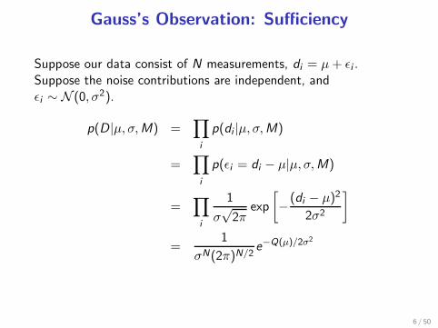
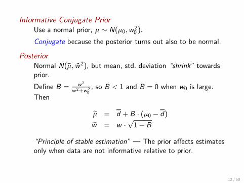
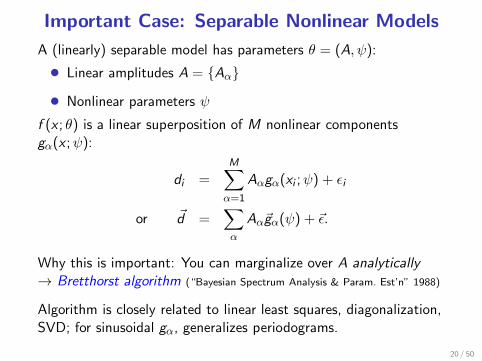
Introduction to Bayesian inference
Lecture 2: Key examples
Tom LoredoDept. of Astronomy, Cornell University
http://www.astro.cornell.edu/staff/loredo/bayes/
CASt Summer School — 5 June 2014
1 / 50
Lecture 2: Key examples
1 Simple examplesNormal DistributionPoisson Distribution
2 Multilevel models for measurement error
3 Bayesian computation
2 / 50
Key examples
1 Simple examplesNormal DistributionPoisson Distribution
2 Multilevel models for measurement error
3 Bayesian computation
3 / 50
Supplement
• Binary classification with binary data
• Bernoulli, binomial, negative binomial distributions
• Parameter estimation & model comparison
• Likelihood principle
• Relationships between probability & frequency
4 / 50
Inference With Normals/Gaussians
Gaussian PDF
p(x |µ, σ) = 1
σ√2π
e−(x−µ)2
2σ2 over [−∞,∞]
Common abbreviated notation: x ∼ N(µ, σ2)
Parameters
µ = 〈x〉 ≡∫
dx x p(x |µ, σ)
σ2 = 〈(x − µ)2〉 ≡∫
dx (x − µ)2 p(x |µ, σ)
5 / 50
Gauss’s Observation: Sufficiency
Suppose our data consist of N measurements, di = µ+ ǫi .Suppose the noise contributions are independent, andǫi ∼ N (0, σ2).
p(D|µ, σ,M) =∏
i
p(di |µ, σ,M)
=∏
i
p(ǫi = di − µ|µ, σ,M)
=∏
i
1
σ√2π
exp
[−(di − µ)2
2σ2
]
=1
σN(2π)N/2e−Q(µ)/2σ2
6 / 50
Find dependence of Q on µ by completing the square:
Q =∑
i
(di − µ)2 [Note: Q/σ2 = χ2(µ)]
=∑
i
d2i +
∑
i
µ2 − 2∑
i
diµ
=
(∑
i
d2i
)+ Nµ2 − 2Nµd where d ≡ 1
N
∑
i
di
= N(µ − d)2 +
(∑
i
d2i
)− Nd
2
= N(µ − d)2 + Nr2 where r2 ≡ 1
N
∑
i
(di − d)2
7 / 50
Likelihood depends on {di} only through d and r :
L(µ, σ) = 1
σN(2π)N/2exp
(−Nr2
2σ2
)exp
(−N(µ − d)2
2σ2
)
The sample mean and variance are sufficient statistics.
This is a miraculous compression of information—the normal dist’nis highly abnormal in this respect!
8 / 50
Estimating a Normal Mean
Problem specificationModel: di = µ+ ǫi , ǫi ∼ N(0, σ2), σ is known → I = (σ,M).
Parameter space: µ; seek p(µ|D, σ,M)
Likelihood
p(D|µ, σ,M) =1
σN(2π)N/2exp
(−Nr2
2σ2
)exp
(−N(µ − d)2
2σ2
)
∝ exp
(−N(µ − d)2
2σ2
)
9 / 50
“Uninformative” priorTranslation invariance ⇒ p(µ) ∝ C , a constant.This prior is improper unless bounded.
Prior predictive/normalization
p(D|σ,M) =
∫dµ C exp
(−N(µ − d)2
2σ2
)
= C (σ/√N)
√2π
. . . minus a tiny bit from tails, using a proper prior.
10 / 50
Posterior
p(µ|D, σ,M) =1
(σ/√N)
√2π
exp
(−N(µ − d)2
2σ2
)
Posterior is N(d ,w2), with standard deviation w = σ/√N .
68.3% HPD credible region for µ is d ± σ/√N.
Note that C drops out → limit of infinite prior range is wellbehaved.
11 / 50
Informative Conjugate PriorUse a normal prior, µ ∼ N(µ0,w
20 ).
Conjugate because the posterior turns out also to be normal.
PosteriorNormal N(µ, w2), but mean, std. deviation “shrink” towardsprior.
Define B = w2
w2+w20, so B < 1 and B = 0 when w0 is large.
Then
µ = d + B · (µ0 − d)
w = w ·√1− B
“Principle of stable estimation” — The prior affects estimatesonly when data are not informative relative to prior.
12 / 50
Conjugate normal examples:
• Data have d = 3, σ/√N = 1
• Priors at µ0 = 10, with w = {5, 2}
0 5 10 15 20x
0.00
0.05
0.10
0.15
0.20
0.25
0.30
0.35
0.40
0.45
p(x|�
)
Prior
LPost.
0 5 10 15 20x
0.00
0.05
0.10
0.15
0.20
0.25
0.30
0.35
0.40
0.45
p(x| �
)
13 / 50
Estimating a Normal Mean: Unknown σ
Supplement: Marginalize over σ → Student’s t distribution
14 / 50
Gaussian Background Subtraction
Measure background rate b = b ± σb with source off.
Measure total rate r = r ± σr with source on.
Infer signal source strength s, where r = s + b.
With flat priors,
p(s, b|D,M) ∝ exp
[−(b − b)2
2σ2b
]× exp
[−(s + b − r)2
2σ2r
]
15 / 50
Marginalize b to summarize the results for s (complete the squareto isolate b dependence; then do a simple Gaussian integral overb):
p(s|D,M) ∝ exp
[−(s − s)2
2σ2s
]s = r − bσ2s = σ2r + σ2
b
⇒ Background subtraction is a special case of backgroundmarginalization; i.e., marginalization “told us” to subtract abackground estimate.
Recall the standard derivation of background uncertainty via“propagation of errors” based on Taylor expansion (statistician’sDelta-method).
Marginalization provides a generalization of errorpropagation—without approximation!
16 / 50
Bayesian Curve Fitting & Least Squares
SetupData D = {di} are measurements of an underlying functionf (x ; θ) at N sample points {xi}. Let fi(θ) ≡ f (xi ; θ):
di = fi(θ) + ǫi , ǫi ∼ N(0, σ2i )
We seek learn θ, or to compare different functional forms(model choice, M).
Likelihood
p(D|θ,M) =
N∏
i=1
1
σi√2π
exp
[−1
2
(di − fi(θ)
σi
)2]
∝ exp
[−1
2
∑
i
(di − fi(θ)
σi
)2]
= exp
[−χ
2(θ)
2
]
18 / 50
Bayesian Curve Fitting & Least Squares
PosteriorFor prior density π(θ),
p(θ|D,M) ∝ π(θ) exp
[−χ
2(θ)
2
]
If you have a least-squares or χ2 code:
• Think of χ2(θ) as −2 logL(θ).
• Bayesian inference amounts to exploration and numericalintegration of π(θ)e−χ2(θ)/2.
19 / 50
Important Case: Separable Nonlinear Models
A (linearly) separable model has parameters θ = (A, ψ):
• Linear amplitudes A = {Aα}
• Nonlinear parameters ψ
f (x ; θ) is a linear superposition of M nonlinear componentsgα(x ;ψ):
di =
M∑
α=1
Aαgα(xi ;ψ) + ǫi
or ~d =∑
α
Aα~gα(ψ) + ~ǫ.
Why this is important: You can marginalize over A analytically→ Bretthorst algorithm (“Bayesian Spectrum Analysis & Param. Est’n” 1988)
Algorithm is closely related to linear least squares, diagonalization,SVD; for sinusoidal gα, generalizes periodograms.
20 / 50
Poisson Dist’n: Infer a Rate from Counts
Problem:Observe n counts in T ; infer rate, r
Likelihood
L(r) ≡ p(n|r ,M) = p(n|r ,M) =(rT )n
n!e−rT
PriorTwo simple standard choices (or conjugate gamma dist’n):
• r known to be nonzero; it is a scale parameter:
p(r |M) =1
ln(ru/rl)
1
r
• r may vanish; require p(n|M) ∼ Const:
p(r |M) =1
ru
21 / 50
Prior predictive
p(n|M) =1
ru
1
n!
∫ ru
0dr(rT )ne−rT
=1
ruT
1
n!
∫ ruT
0d(rT )(rT )ne−rT
≈ 1
ruTfor ru ≫ n
T
PosteriorA gamma distribution:
p(r |n,M) =T (rT )n
n!e−rT
22 / 50
Gamma Distributions
A 2-parameter family of distributions over nonnegative x , withshape parameter α and scale parameter s:
pΓ(x |α, s) =1
sΓ(α)
(xs
)α−1e−x/s
Moments:
E(x) = sα Var(x) = s2α
Our posterior corresponds to α = n+ 1, s = 1/T .
• Mode r = nT; mean 〈r〉 = n+1
T(shift down 1 with 1/r prior)
• Std. dev’n σr =√
n+1T
; credible regions found by integrating (canuse incomplete gamma function)
23 / 50
The flat priorBayes’s justification: Not that ignorance of r → p(r |I ) = C
Require (discrete) predictive distribution to be flat:
p(n|I ) =
∫dr p(r |I )p(n|r , I ) = C
→ p(r |I ) = C
Useful conventions
• Use a flat prior for a rate that may be zero
• Use a log-flat prior (∝ 1/r) for a nonzero scale parameter
• Use proper (normalized, bounded) priors
• Plot posterior with abscissa that makes prior flat
25 / 50
The On/Off Problem
Basic problem
• Look off-source; unknown background rate bCount Noff photons in interval Toff
• Look on-source; rate is r = s + b with unknown signal sCount Non photons in interval Ton
• Infer s
Conventional solution
b = Noff/Toff ; σb =√Noff/Toff
r = Non/Ton; σr =√Non/Ton
s = r − b; σs =√σ2r + σ2
b
But s can be negative!
26 / 50
Spectrum of Ultrahigh-Energy Cosmic Rays
Nagano & Watson 2000
HiRes Team 2007
log10(E) (eV)F
lux*
E3 /1
024 (
eV2 m
-2 s
-1 s
r-1)
AGASAHiRes-1 MonocularHiRes-2 Monocular
1
10
17 17.5 18 18.5 19 19.5 20 20.5 21
28 / 50
N is Never Large
Sample sizes are never large. If N is too small to get asufficiently-precise estimate, you need to get more data (or makemore assumptions). But once N is ‘large enough,’ you can startsubdividing the data to learn more (for example, in a publicopinion poll, once you have a good estimate for the entire country,you can estimate among men and women, northerners andsoutherners, different age groups, etc etc). N is never enoughbecause if it were ‘enough’ you’d already be on to the nextproblem for which you need more data.
— Andrew Gelman (blog entry, 31 July 2005)
29 / 50
N is Never Large
Sample sizes are never large. If N is too small to get asufficiently-precise estimate, you need to get more data (or makemore assumptions). But once N is ‘large enough,’ you can startsubdividing the data to learn more (for example, in a publicopinion poll, once you have a good estimate for the entire country,you can estimate among men and women, northerners andsoutherners, different age groups, etc etc). N is never enoughbecause if it were ‘enough’ you’d already be on to the nextproblem for which you need more data.
Similarly, you never have quite enough money. But that’s anotherstory.
— Andrew Gelman (blog entry, 31 July 2005)
29 / 50
Bayesian Solution to On/Off Problem
First consider off-source data; use it to estimate b:
p(b|Noff , Ioff ) =Toff(bToff)
Noff e−bToff
Noff !
Use this as a prior for b to analyze on-source data. For on-sourceanalysis Iall = (Ion,Noff , Ioff):
p(s, b|Non) ∝ p(s)p(b)[(s + b)Ton]None−(s+b)Ton || Iall
p(s|Iall) is flat, but p(b|Iall) = p(b|Noff , Ioff), so
p(s, b|Non, Iall) ∝ (s + b)NonbNoff e−sTone−b(Ton+Toff )
30 / 50
Now marginalize over b;
p(s|Non, Iall) =
∫db p(s, b | Non, Iall)
∝∫
db (s + b)NonbNoff e−sTone−b(Ton+Toff )
Expand (s + b)Non and do the resulting Γ integrals:
p(s|Non, Iall) =
Non∑
i=0
Ci
Ton(sTon)ie−sTon
i !
Ci ∝(1 +
Toff
Ton
)i(Non + Noff − i)!
(Non − i)!
Posterior is a weighted sum of Gamma distributions, each assigning adifferent number of on-source counts to the source. (Evaluate viarecursive algorithm or confluent hypergeometric function.)
31 / 50
Supplement: Two more solutions of on/off problem (includingdata augmentation); multibin case
34 / 50
Recap of Key Ideas From Examples
• Sufficient statistic: Model-dependent summary of data
• Conjugate priors
• Marginalization: Generalizes background subtraction,propagation of errors
• Exact treatment of Poisson background uncertainty (don’tsubtract!)
• Likelihood principle
• Student’s t for handling σ uncertainty
35 / 50
Key examples
1 Simple examplesNormal DistributionPoisson Distribution
2 Multilevel models for measurement error
3 Bayesian computation
36 / 50
Complications With Survey Data
• Selection effects (truncation, censoring) — obvious (usually)Typically treated by “correcting” dataMost sophisticated: product-limit estimators
• “Scatter” effects (measurement error, etc.) — insidiousTypically ignored (average out???)
37 / 50
Many Guises of Measurement ErrorAuger data above GZK cutoff (PAO 2007; Soiaporn+ 2013)
QSO hardness vs. luminosity (Kelly 2007, 2012)
38 / 50
Accounting For Measurement ErrorIntroduce latent/hidden/incidental parameters
Suppose f (x |θ) is a distribution for an observable, x .
From N precisely measured samples, {xi}, we can infer θ from
L(θ) ≡ p({xi}|θ) =∏
i
f (xi |θ)
p(θ|{xi}) ∝ p(θ)L(θ) = p(θ, {xi})
(A binomial point process)
39 / 50
Graphical representation
• Nodes/vertices = uncertain quantities (gray → known)
• Edges specify conditional dependence
• Absence of an edge denotes conditional independence
θ
x1 x2 xN
Graph specifies the form of the joint distribution:
p(θ, {xi}) = p(θ) p({xi}|θ) = p(θ)∏
i
f (xi |θ)
Posterior from BT: p(θ|{xi}) = p(θ, {xi})/p({xi})40 / 50
But what if the x data are noisy, Di = {xi + ǫi}?
{xi} are now uncertain (latent) parametersWe should somehow incorporate ℓi(xi ) = p(Di |xi ):
p(θ, {xi}, {Di}) = p(θ) p({xi}|θ) p({Di}|{xi})= p(θ)
∏
i
f (xi |θ) ℓi (xi )
Marginalize over {xi} to summarize inferences for θ.Marginalize over θ to summarize inferences for {xi}.
Key point: Maximizing over xi and integrating over xi can givevery different results!
41 / 50
To estimate x1:
p(x1|{x2, . . .}) =
∫dθ p(θ) f (x1|θ) ℓ1(x1)×
N∏
i=2
∫dxi f (xi |θ) ℓi (xi)
= ℓ1(x1)
∫dθ p(θ) f (x1|θ)Lm,1(θ)
≈ ℓ1(x1)f (x1|θ)
with θ determined by the remaining data.
f (x1|θ) behaves like a prior that shifts the x1 estimate away fromthe peak of ℓ1(xi ).
This generalizes the corrections derived by Eddington, Malmquistand Lutz-Kelker.
Landy & Szalay (1992) proposed adaptive Malmquist correctionsthat can be viewed as an approximation to this.
42 / 50
Graphical representation
DND1 D2
θ
x1 x2 xN
p(θ, {xi}, {Di}) = p(θ) p({xi}|θ) p({Di}|{xi})= p(θ)
∏
i
f (xi |θ) p(Di |xi ) = p(θ)∏
i
f (xi |θ) ℓi(xi )
A two-level multi-level model (MLM).
43 / 50
Bayesian MLMs in Astronomy
Surveys (number counts/“logN–log S”/Malmquist):
• GRB peak flux dist’n (Loredo & Wasserman 1998)
• TNO/KBO magnitude distribution (Gladman+ 1998;Petit+ 2008)
• MLM tutorial; Malmquist-type biases in cosmology(Loredo & Hendry 2009 in BMIC book)
• “Extreme deconvolution” for proper motion surveys(Bovy, Hogg, & Roweis 2011)
Directional & spatio-temporal coincidences:
• GRB repetition (Luo+ 1996; Graziani+ 1996)
• GRB host ID (Band 1998; Graziani+ 1999)
• VO cross-matching (Budavari & Szalay 2008)
44 / 50
Time series:
• SN 1987A neutrinos, uncertain energy vs. time (Loredo& Lamb 2002)
• Multivariate “Bayesian Blocks” (Dobigeon, Tourneret &Scargle 2007)
• SN Ia multicolor light curve modeling (Mandel+ 2009,2011)
Linear & nonlinear regression with measurement error:
• QSO hardness vs. luminosity (Kelly 2007, 2012)
• Dust SEDs (Kelly+ 2012)
More information:http://astrostatistics.psu.edu/su10/surveys.html
Overview of MLMs in astronomy: arXiv:1208.3036In progress: GPU software (Budavari, Kelly, TJL)
45 / 50
Key examples
1 Simple examplesNormal DistributionPoisson Distribution
2 Multilevel models for measurement error
3 Bayesian computation
46 / 50
Statistical IntegralsInference with independent data
Consider N data, D = {xi}; and model M with m parameters.
Suppose L(θ) = p(x1|θ) p(x2|θ) · · · p(xN |θ).
Frequentist integralsFind long-run properties of procedures via sample spaceintegrals:
I(θ) =∫
dx1 p(x1|θ)∫
dx2 p(x2|θ) · · ·∫
dxN p(xN |θ)f (D, θ)
Rigorous analysis must explore the θ dependence; rarely donein practice.
“Plug-in” approximation: Report properties of procedure forθ = θ. Asymptotically accurate (for large N, expect θ → θ).
“Plug-in” results are easy via Monte Carlo (due toindependence).
47 / 50
Bayesian integrals∫dmθ g(θ) p(θ|M)L(θ) =
∫dmθ g(θ) q(θ)
p(θ|M)L(θ)
• g(θ) = 1 → p(D|M) (norm. const., model likelihood)
• g(θ) = ‘box’ → credible region
• g(θ) = θ → posterior mean for θ
Such integrals are sometimes easy if analytic (especially in lowdimensions), often easier than frequentist counterparts (e.g.,normal credible regions, Student’s t).
Asymptotic approximations: Require ingredients familiarfrom frequentist calculations. Bayesian calculation is notsignificantly harder than frequentist calculation in this limit.
Numerical calculation: For “large” m (> 4 is often enough!)the integrals are often very challenging because of structure(e.g., correlations) in parameter space. This is usually pursuedwithout making any procedural approximations.
48 / 50
Bayesian ComputationLarge sample size: Laplace approximation
• Approximate posterior as multivariate normal → det(covar) factors• Uses ingredients available in χ2/ML fitting software (MLE, Hessian)• Often accurate to O(1/N)
Modest-dimensional models (d<∼10 to 20)
• Adaptive cubature• Monte Carlo integration (importance & stratified sampling, adaptive
importance sampling, quasirandom MC)
High-dimensional models (d>∼5)
• Posterior sampling — create RNG that samples posterior• MCMC is most general framework — Murali Haran’s lab
49 / 50
See SCMA 5 Bayesian Computation tutorial notes,and notes from next week’s sessions,for more on MLMs & computation!
See online resource list for an annotated listof Bayesian books and software
50 / 50