Introduction to biophysics

Bert Kappen,

Department of BiophysicsRadboud University Nijmegen

February 7, 2008

1

Contents

1 Preface 4

2 Introduction to neurons and the brain 52.1 Nerve cells . . . . . . . . . . . . . . . . . . . . . . . . . . . . . 52.2 The nervous system . . . . . . . . . . . . . . . . . . . . . . . . 82.3 Some features of the cortex . . . . . . . . . . . . . . . . . . . 122.4 Summary . . . . . . . . . . . . . . . . . . . . . . . . . . . . . 182.5 Exercises . . . . . . . . . . . . . . . . . . . . . . . . . . . . . . 18

3 Electrical properties of cells 193.1 Ion channels . . . . . . . . . . . . . . . . . . . . . . . . . . . . 203.2 The Nernst equation . . . . . . . . . . . . . . . . . . . . . . . 213.3 The Goldman equation . . . . . . . . . . . . . . . . . . . . . . 233.4 The Nernst-Planck equation . . . . . . . . . . . . . . . . . . . 243.5 The Hodgkin-Katz experiments . . . . . . . . . . . . . . . . . 27

3.5.1 The role of K+ . . . . . . . . . . . . . . . . . . . . . . 273.5.2 The role of Na+ . . . . . . . . . . . . . . . . . . . . . . 283.5.3 Permeability changes during action potential . . . . . . 30

3.6 Summary . . . . . . . . . . . . . . . . . . . . . . . . . . . . . 333.7 Exercises . . . . . . . . . . . . . . . . . . . . . . . . . . . . . . 33

4 The Hodgkin-Huxley model of action potentials 364.1 The voltage clamp technique . . . . . . . . . . . . . . . . . . . 364.2 Two types of voltage dependent ionic currents . . . . . . . . . 364.3 The Hodgkin-Huxley model . . . . . . . . . . . . . . . . . . . 43

4.3.1 The K+ conductance . . . . . . . . . . . . . . . . . . . 484.3.2 The Na+ conductance . . . . . . . . . . . . . . . . . . 504.3.3 Action potentials . . . . . . . . . . . . . . . . . . . . . 51

4.4 Spike propagation . . . . . . . . . . . . . . . . . . . . . . . . . 534.4.1 Passive current flow . . . . . . . . . . . . . . . . . . . . 534.4.2 Spike propagation . . . . . . . . . . . . . . . . . . . . . 574.4.3 Myelin . . . . . . . . . . . . . . . . . . . . . . . . . . . 60

4.5 Summary . . . . . . . . . . . . . . . . . . . . . . . . . . . . . 644.6 Exercises . . . . . . . . . . . . . . . . . . . . . . . . . . . . . . 64

2

5 Synapses 675.1 Introduction . . . . . . . . . . . . . . . . . . . . . . . . . . . . 675.2 Chemical synapses . . . . . . . . . . . . . . . . . . . . . . . . 675.3 The post-synaptic potential . . . . . . . . . . . . . . . . . . . 685.4 Stochastic PSPs . . . . . . . . . . . . . . . . . . . . . . . . . . 725.5 Learning . . . . . . . . . . . . . . . . . . . . . . . . . . . . . . 745.6 Long term potentiation . . . . . . . . . . . . . . . . . . . . . . 775.7 Hebbian learning . . . . . . . . . . . . . . . . . . . . . . . . . 78

5.7.1 Ocular dominance . . . . . . . . . . . . . . . . . . . . . 795.8 Summary . . . . . . . . . . . . . . . . . . . . . . . . . . . . . 815.9 Exercises . . . . . . . . . . . . . . . . . . . . . . . . . . . . . . 81

6 Perceptrons 826.1 Threshold units . . . . . . . . . . . . . . . . . . . . . . . . . . 826.2 Linear separation . . . . . . . . . . . . . . . . . . . . . . . . . 836.3 Perceptron learning rule . . . . . . . . . . . . . . . . . . . . . 84

6.3.1 Convergence of Perceptron rule . . . . . . . . . . . . . 866.4 Linear units . . . . . . . . . . . . . . . . . . . . . . . . . . . . 88

6.4.1 Gradient descent learning . . . . . . . . . . . . . . . . 896.4.2 The value of η . . . . . . . . . . . . . . . . . . . . . . . 90

6.5 Non-linear units . . . . . . . . . . . . . . . . . . . . . . . . . . 916.6 Multi-layered perceptrons . . . . . . . . . . . . . . . . . . . . 926.7 Summary . . . . . . . . . . . . . . . . . . . . . . . . . . . . . 956.8 Exercises . . . . . . . . . . . . . . . . . . . . . . . . . . . . . . 95

3

1 Preface

This introductory course on biophysics introduces the principles of electricalexcitability of cell membranes, which form the basis of all information pro-cessing in the nervous system. The course covers some of the classical results,such as cellular membranes, ionic currents, equilibrium behavior and actionpotentials. The course is intended for physics students and will thereforehave an emphasis on physical modeling.

Section 2 is an introductory chapter, where I will give an overview ofsome of the basic anatomical properties of the nervous system and of nervecells and discuss the spiking behavior of nerve cells and their functionalrelevance. In section 3, I will discuss the stationary behavior of the cell, suchas the relation between ionic concentrations inside and outside the cell, theionic currents and the membrane potential. In section 4, I will discuss themechanism for action potential generation, spike propagation, linear cabletheory and the role of myelin. In section 5, I will discuss synapses and someaspects of learning. In section 6, I will give a brief introduction to a class ofpopular neural networks, the (multi-layered) perceptrons.

Bert KappenNijmegen, January 2007

4

2 Introduction to neurons and the brain

Perhaps the major reason that neuro science is such an exciting field is thewealth of fundamental questions about the human brain (and the rest of thenervous system) that remain unanswered. Such understanding entails unrav-eling the interconnections of large numbers of nerve cells, that are organizedinto systems and subsystems.

The fact that cells are the basic element of living organisms was recog-nized early in the nineteenth century. It was not until well into the twen-tieth century, however, that neuro scientists agreed that nervous tissue, likeall other organs is made up of these fundamental units. Santiago Ramony Cajal argued persuasively that nerve cells are discrete entities and thatthey communicate with one another by means of specialized contacts calledsynapses. The human brain is estimated to contain 100 billion neurons andseveral times as many supporting cells, called neuroglial cells.

2.1 Nerve cells

In most respects, the structure of neurons resembles that of other cells. Eachcell has a cell body containing a nucleus, endoplasmic reticulum, ribosomes,Golgi apparatus, mitochondria, and other organelles that are essential to thefunction of all cells (see fig. 2). Specific for nerve cells, is their dendriticstructure (see fig. 3. The dendrites (together with the cell body) providesites for the synaptic contacts made by the terminals of other nerve cells andcan thus be regarded as specialized for receiving information. The numberof inputs that a particular neuron receives depends on the complexity ofits dendrite and can range from 1 to about 100.000. The information fromthe inputs that impinge on the dendrites is ’read out’ at the border of thecell body and the axon. The axon is an extension that may reach from afew hundred micrometers to a meter. Typical axons in the brain a a fewmillimeters long. Axons in the spinal cord are about a meter long. Theaxon carries electrical signals over such distances through action potentials,a self-generating electrical wave that propagates from the cell body to theend of the axon.

The information encoded by action potentials is passed on to the next cellby means of synaptic transmission. The arrival of the action potential causesthe release of neurotransmitters, which in turn modify the electrical proper-ties of the post-synaptic cell. The net effect is a change of the membrane

5

Figure 1: The brain consists of network of neurons (Ramon y Cajal, 1910).Shown is one of the original Golgi stain images of rat cortex. Only a smallfraction of neurons are stained with this technique.

6

Figure 2: The major light and electron microscopical features of neurons.A) Diagram of nerve cells and their component parts. B) Axon initial seg-ment (blue) entering a myelin sheath (gold). C) Terminal boutons (blue)loaded with synaptic vesicles (arrowheads) forming synapses (arrows) with adendrite (purple). D) Transverse section of axons (blue) ensheathed by theprocesses of oligodendrocytes (gold). E) Apical dendrites (purple) of corticalpyramidal cells. F) Nerve cell bodies (purple) occupied by large round nu-clei. G) Portion of a myelinated axon (blue) illustrating the intervals betweenadjacent segments of myelin (gold) referred to as nodes of Ranvier (arrows).

7

Figure 3: Cells stained with silver salts (Golgi stain). * indicates axon. a)muscle cell b-d) retinal cells e) Cortical pyramidal cell f) Cerebellar Purkinjecell

potential of the post-synaptic cell.It is thought, that glia cells do not play a primary role in information

processing in the brain. The different types of glia cells have two impor-tant functions. The astrocytes maintain in a variety of ways the appropriatechemical environment for the nerve cells. The oligodendrocytes or Schwanncells lay down a laminated wrapping called myelin around some, but not all,axons, which has important effects on the speed of action potential propaga-tion.

2.2 The nervous system

The nervous system is traditionally divided into a central and peripheralcomponent (see fig. 4). The peripheral system contains the sensory neurons,which receive information from the outside world, and the motor neurons,that connect to muscles and glands. Sensory information is processed in

8

Figure 4: The major components of the nervous system and their functionalrelationships. A) The CNS (brain and spinal cord) and the PNS (spinal andcranial nerves). B) The peripheral nervous system receives sensory inputand outputs motor commands. The central nervous system provides the’mapping’ from sensory input to motor output.

the brain, with the ultimate goal to generate the appropriate motor actions.Nerve cells that carry information toward the central nervous system arecalled afferent neurons, nerve cells that carry information away from thebrain are called efferent neurons. Nerve cells that only participate in thelocal aspects of a circuit are called inter-neurons. The simple spinal reflexcircuit in fig. 5 illustrates this terminology.

The central nervous system is usually considered to include seven basicparts (see fig. 6): the spinal cord; the medulla, the pons and the midbrain(collectively called the brainstem); the cerebellum; the diencephalon and thecerebral hemispheres (collectively called the forebrain).

The thalamus relays information to the cerebral cortex from other partsof the brain. Specialized substructures of the thalamus are engaged in motorfunctions and reproduction and hormone secretion. The brainstem containsstructures, such as the superior colliculus that is involved in eye movement.The major function of the cerebellum is coordination of motor activity, pos-ture and equilibrium. Like the cerebral cortex, the cerebellum is coveredby a thin cortex. Another important area of the central nervous system isthe hippocampus which is thought to be involved in the storage of episodicmemories. It is not visible in fig. 6, since it is located centrally.

9

Figure 5: A simple reflex circuit, the knee-jerk response, illustrates severalpoints about the functional organization of neural circuits. Stimulation of amuscle stretch receptor initiates action potentials that travel centrally alongthe afferent axons of the sensory neurons. This information stimulates spinalmotor neurons by means of synaptic contacts. The action potentials gen-erated in motor neurons travel peripherally in efferent axons, giving rise tomuscle contraction. Bottom) Relative frequency of action potentials (in-dicated by individual vertical lines). Notice the modulatory effect of theinterneuron.

10

Figure 6: A) The terms anterior, posterior, superior, and inferior refer tothe long axis of the body. B) The major planes of section used in cuttingor imaging the brain. C) The subdivisions and components of the centralnervous system.

11

Figure 7: Structure of the human neocortex. A) summary of the cellularcomposition of the six layers of the neocortex. B) Based on variations inthickness, cell density and other histological features of the six neo-corticallaminae, the neocortex can be divided into areas (Brodmann 1909). Theseanatomical distinctions have later been shown to relate to different functions.Red indicates the primary motor cortex, blue the primary somatic sensorycortex, green the primary auditory cortex and yellow the primary visualcortex. All other Brodmann areas are considered association cortex.

2.3 Some features of the cortex

The cerebral hemispheres, also called the cerebral cortex are two convolutedsheets of neural tissue of about 2 mm thickness and spreads over about11 dm2 each. The sheets are connected through the corpus callosum (800million fibers). The cortical sheet contains six layers that can be identifiedanatomically (fig. 7a). This structure of six layers is remarkably uniformthrough the cortex. Local differences has lead to the classification of thecortex into cortical areas (see fig. 7b).

The cortical tissue consists for about 80 % of pyramidal cells (fig. 3) andthe remainder are so called inter-neurons. There are two types of pyramidalneurons, the upper pyramidal neurons lying in layers II and III and the lowerpyramidal neurons which we find mainly in layer V. Both receive their inputsignals from stellate cells, which are inter-neurons lying in layer IV. The lowerpyramidal neurons are output neurons; their axons make contact with thethalamus. The upper pyramidal neurons make distant connections with thepyramidal cells of other cortical areas. The six layer structure is schematically

12

Figure 8: Canonical neo-cortical circuitry. Green arrows indicate outputs tothe major targets of each of the neo-cortical layers in humans; orange arrowindicates thalamic input (primarily to layer IV); purple arrows indicate inputfrom other cortical areas: and blue arrows indicate input from the brainstemto each layer.

drawn in fig. 8.Neurons in the sensory parts of the cortex, such as the visual, auditory

or somatic sensory cortex, respond selectively to stimuli from the outsideworld. This gives rise to the notion of a receptive field of a neuron, which isthe collection of all stimuli that elicit an electrical response in that neuron. InFig. 9 we see an example of a somatosensory receptive field. The use of micro-electrodes to record action potential activity for different stimuli, provides acell-by-cell analysis of the receptive field of each cell and the organization oftopographic maps. In Fig. 10, we see an example of a visual receptive field.Some neurons in the visual cortex respond selectively to the orientation of alight bar. Each neuron has its preferred orientation.

Nearby pyramidal cells can make direct excitatory synaptic connectionsor indirect inhibitory connections by connecting to an inhibitory interneu-ron, which in turn connects to another pyramidal cell. The probability ofconnection is very high for nearby pyramidal neurons and drops off at about30 µm. Therefore, neurons within a cortical column, which is a cross-sectionof the cortical sheet of about this diameter, display strongly correlated ac-

13

Figure 9: Single-unit electrophysiological recording from cortical pyramidalneuron, showing the firing pattern in response to a specific peripheral stim-ulus. A) Typical experimental set-up. B) Defining neuronal receptive fields.

Figure 10: Neurons in the visual cortex respond selectively to oriented edges.A) An anesthetized cat focuses on a screen, where images can be projected; anextracellular electrode records the responses of neurons in the visual cortex.B) Neurons in the visual cortex typically respond vigorously to a bar of lightoriented at a particular angle and weakly (or not at all) to other orientations.

14

Figure 11: A) Ocular dominance stripes in LGN and layer IV primary visualcortex. B) Pattern of ocular dominance columns in human striate cortex.

tivity. The result is that nearby neurons have similar functional roles. Anexample is ocular dominance given in fig. 11. The lateral geniculate nucleus(LGN) receives inputs from both eyes, but this information is segregated inseparate layers. In many species, including most primates, the inputs fromthe two eyes remain segregated in the ocular dominance columns of layer IV,the primary cortical target of LGN axons. Layer IV neurons send their axonsto other cortical layers; it is at this stage that the information from the twoeyes converges onto individual neurons.

Such correlated activity can also be measured in vivo. Fig. 12 shows thatneurons in the same column have identical orientation preference. Neurons innearby columns have similar orientation preference. Thus, this part of visualcortex displays a topographical map, meaning that stimulus features (in thiscase the orientation) are mapped continuously onto the spatial location inthe cortex.

Cortical maps are found throughout the sensory cortices and motor cor-tex. Fig. 13 shows that nearby neurons in the auditory cortex respond prefer-entially to nearby frequencies. Typically, maps are deformed representations,that use more neurons to represent important regions. In fig. 14 shows theexample of the somatotopic order in the human primary somatic sensorycortex.

15

Figure 12: Columnar organization of orientation selectivity in the monkeystriate cortex. Vertical electrode penetrations encounter neurons with thesame preferred orientations, whereas oblique penetrations show a systematicchange in orientation across the cortical surface.

Figure 13: The human auditory cortex. A) Diagram showing the brain inleft lateral view. The primary auditory cortex (A1) is shown in blue. B) Theprimary auditory cortex has a tonotopic organization.

16

Figure 14: Somatotopic order in the human primary somatic sensory cor-tex. A) approximate region of human cortex from which electrical activityis recorded following mechanosensory stimulation of different parts of thebody. B)Somatotopic representation of the whole body. C) Cartoon of thehomunculus constructed on the basis of such mapping. The amount of so-matic sensory cortex devoted to hands and face is much larger than therelative amount of body surface in these regions.

17

2.4 Summary

Although the human brain is often discussed as if it were a single organ,it contains a large number of systems and subsystems. Various types ofneurons in these systems are assembled into interconnected circuits that relayand process the electrical signals that are the basis of all neural functions.Sensory components of the nervous system supply information to the centralnervous system about the internal and external environment. The integratedeffects of central processing are eventually translated into action by the motorcomponents. The material in this chapter is largely based on [1].

2.5 Exercises

1. Propose a neuron with its input dendritic tree connected to the retina,such that the neuron has the receptive field property as observed infigure 10.

2. Think about a neural network that may cause the occular dominancepatterns observed in figure 11.

(a) Consider the strenght and sign of the forward connections fromthe eyes to the cortex.

(b) The lateral connections within the cortex are typically of the Mex-ican hat type: short range excitatory connections and long rangeinhibitory connections. Explain their role.

3. Suppose you were a neuron and you could only communicate with yourfellow neurons through the emission of action potentials. How wouldyou do it? Describe two ways and discuss their respective advantageand disadvantages.

18

Figure 15: Recording passive and active electrical signals in a nerve cell.

3 Electrical properties of cells

Nerve cells generate electrical signals that transmit information. Neuronsare not good conductors of electricity, but have evolved elaborate mecha-nisms for generating electrical signals based on the flow of ions across theirmembranes. Ordinarily, neurons generate a negative potential, called theresting membrane potential , that can be measured by intracellular record-ing. The action potential is a short spike in the membrane potential, makingthe membrane potential temporarily positive. Action potentials are propa-gated along the length of axons and are the fundamental electrical signal ofneurons. Generation of both the resting potential and the action potentialcan be understood in terms of the nerve cell’s selective permeability to dif-ferent ions and the relative concentrations of these ions inside and outsidethe cell.

The best way to observe an action potential is to use an intracellularmicroelectrode to record directly the electrical potential across the neuronalmembrane (fig. 15). Two micro-electrodes are inserted into a neuron, one ofthese measures the membrane potential while the other injects current intothe neuron. Inserting the voltage-measuring microelectrode into the neuronreveals a negative potential, the resting membrane potential. Typical valuesare -60-80 mV. Injecting current through the current-passing microelectrodealters the neuronal membrane potential. Hyper-polarizing current pulsesdecrease the membrane potential and produce only passive changes in themembrane potential. Depolarizing currents increase the membrane potential.

19

Figure 16: Ion pumps and ion channels are responsible for ionic movementsacross neuronal membranes.

Small currents evoke a passive response. Currents that exceed a thresholdvalue, evoke an action potential. Action potentials are active responses in thesense that they are generated by changes in the permeability of the neuronalmembrane.

3.1 Ion channels

Electrical potentials are generated across the membranes of neurons (in factof all cells) because (1) there are difference in the concentrations of specificions across nerve cell membranes and (2) the membranes are selectively per-meable to some of these ions (fig. 16). The ion concentration gradients areestablished by proteins known as ion pumps, which actively move ions into orout of cells against their concentration gradients. The selective permeabilityof membranes is due largely to ion channels, proteins that allow only certainkinds of ions to cross the membrane in the direction of their concentrationgradients. Thus, channels and pumps basically work against each other, andin so doing they generate cellular electricity.

Membrane channels can open or close in response to changes in their di-rect vicinity, such as a change in the membrane potential, changes in theconcentration of neurotransmitters, or sensory input. For instance, hair cellsin the cochlea (inner ear) mechanically deform in response to sound, and this

20

Figure 17: Open-shut gating of an ionic channel showing 8 brief openings.The probability of opening depends on many factors. At -140 mV appliedmembrane potential, one open channel passes 6.6 pA, corresponding to a flowof 4.1× 107 ions per second.

mechanical deformation changes the permeability of certain channels. Chan-nels open and close rapidly in a stochastic manner (fig. 17). The macroscop-ically observed permeability of the membrane is related to the probabilitythat the channel is open.

3.2 The Nernst equation

Consider a simple system in which an imaginary membrane separates twocompartments containing solutions of ions. Let both compartments containan amount of potassium ions (K+) and an equal amount of some negativelycharged ions A−, such that both compartments are electrically neutral. Sup-pose that the membrane is permeable only to potassium ions. If the con-centration of K+ on each side of the membrane is equal, then no electricalpotential across it will be measured. However, if the concentration of K+ isnot the same on the two sides (and thus the concentrations of A− differ aswell, but these cannot move), then the potassium ions will flow down theirconcentration gradient and take their electrical charge with them as they go.Therefore, an electrical potential will be generated, which will drive K+ ionsin the reverse direction. An electrochemical equilibrium will be reached whenthe diffusive force equals the electromotive force (fig. 18). The positive andnegative charge excess in both compartments will concentrate against themembrane (why?) like a capacitor. We thus conclude that the equilibriumpotential difference will be an increasing function of the ratio of concentra-tions of K+ in the two compartments.

The electrochemical equilibrium can be quantitatively described by theBoltzmann statistics, which states that the probability P to encounter a

21

Figure 18: A-B) Electrochemical equilibrium due to selective permeabilityto K+ ions. Concentration gradient drives K+ ions to the right establishing acharge difference. In equilibrium the ionic current due to the concentrationdifference balances the current in the reverse direction due to the electricalpotential difference. C) The relationship between the transmembrane con-centration gradient and the membrane potential as predicted by the Nernstequation Eq. 1

system in equilibrium in a state with energy u is proportional to

P ∝ exp(− u

kT

)= exp

(− U

RT

)

with u the potential energy per ion, k is the Boltzmann constant and Tis the absolute temperature. U = NAu is the potential energy per mole;NA = 6.022 × 1023 mol−1 is Avogadro’s number; and R = kNA = 8.314 Jmol−1 K−1 is the Gas constant.

The charged ions S that can move freely through the membrane can bein two states: in the left or right compartment, which we denote by l and r,respectively. The potential energy is proportional to the electric potential Vand thus the potential energy per mole of an ion of valence zS is given by

Ul,r = zSeNAVl,r = zSFVl,r

with e the unit of electric charge and F = eNA = 9.648 × 104 C mol−1 iscalled the Faraday constant.

Thus, for a given electrical potentials Vl and Vr in the left and rightcompartment, we can compute the relative probability to encounter an S ion

22

left or right:

PlPr

=exp(−zSFVl/RT )

exp(−zSFVr/RT )= exp

(−zSFRT

(Vl − Vr))

The concentration of ions in the left and right compartment, [S]l,r, is pro-portional to the probability Pl,r. We can invert the above expression andexpress the difference in electrical potential in terms of the concentrations:

VNernst = Vl − Vr =RT

zSFln

[S]r[S]l

(1)

This expression is knows as the Nernst equation and describes both the equi-librium concentration ratio when we apply an external potential difference,as well as the equilibrium potential difference when we consider the abovesystem at fixed concentration differences. The Nernst potential depends ontemperature, the concentration ratio and valence of the freely moving ions.In practice, it is often useful the replace the natural logarithm by the base-10logarithm: ln = 2.3 log10. Then

VNernst =1

zSlog10

([S]r[S]l

)× 58mV

at T = 200C.For biological membranes, the K+ concentration is typically much higher

inside the cell than outside the cell. A typical ratio is [K+]out : [K+]in = 1 : 10,yielding a Nernst potential of -58 mV.

The number of ions that needs to flow to generate the electrical potentialis very small (exercise). This means that the movement of ions required toreach the Nernst potential 1) hardly affects the neutrality of the intra- andextracellular media and 2) do not require much pumping by the ion pumps.

3.3 The Goldman equation

The Nernst equation accurately describes the relation between ion concen-trations and the membrane potential, when only one type of ion can movethrough the membrane. In reality, many types of ions are present in the in-tra and extracellular medium, each of which has its own permeability. Somerealistic numbers are given in table 1. For instance, imagine what wouldhappen if the intracellular K+ and Na+ concentrations are 100 mM and 10

23

Ion Intracellular Extracellular

Squid axonK+ 400 20Na+ 50 440Cl− 40-150 560

Ca2+ 0.0001 10

Mammalian neuronK+ 140 5Na+ 5-15 145Cl− 4-30 110

Ca2+ 0.0001 1-2

Table 1: Extracellular and intracellular ion concentrations in millimole perliter (mM).

mM, respectively and the extracellular concentrations of K+ and Na+ are re-versed: 10 mM for K+ and 100 mM for Na+. If the membrane would be onlypermeable to K+, the membrane potential would be -58 mV. If the membranewould be only permeable to Na+, the membrane potential would be +58 mV.What will happen if the membrane is partially permeable for both ions?

For the case most relevant to neurons, in which K+, Na+ and Cl− are theprimary permeant ions, the general solution, called the Goldman equation,was developed by David Goldman in 1943:

V = log10

(PK+[K+]r + PNa+[Na+]r + PCl−[Cl−]lPK+[K+]l + PNa+[Na+]l + PCl−[Cl−]r

)× 58mV (2)

where V is the equilibrium voltage across the membrane, and the Pi, i =K+,Na+,Cl− are the permeabilities of the three types of ions. We see thatin the case that the membrane is only permeable to one ion, the Goldmanequation reduces to the Nernst equation. In the following subsection, we willderive the Goldman equation.

3.4 The Nernst-Planck equation

Consider a membrane of thickness a and let x = 0 to x = a denote theoutside and inside of the membrane, respectively. Let the electrical potentialbe Vout = V (0) = 0 and Vin = V (a) = V . Let us assume that we have

24

a number of different ions, labeled by i, each with its own concentrationCi(x) and valence zi. The extracellular and intracellular concentrations aredenoted by

[Ci]out = Ci(0), [Ci]in = Ci(a) (3)

Due to the potential difference and the concentration differences, ions willflow through the membrane. The electric force per ion of type i is −ziedV (x)

dx.

The number of ions per liter is NACi(x), with Ci(x) in units of mol per liter.Therefore, the electric force per unit volume is

−ziCi(x)FdV (x)

dx

The diffusive force on ion i per unit volume is proportional to the con-centration gradient as well as the absolute temperature. Multiplying by theGas constant gives the diffusive force

−RT dCi(x)

dx

in units of Newton per liter.The force on the ions is the sum of the electric and diffusive force and

results in a movement of the ions proportional to the mobility ui of the ions.The mobility will be soon related to the specific permeability of the membraneto each of the ions. The direction of movement is in the direction of theforce, but the direction of charge depends again on the valence. Therefore,the current for ions i is:

Ii = uizi

(−RT dCi(x)

dx− ziCi(x)F

dV (x)

dx

)(4)

Eq. 4 is a differential equation in Ci(x), given the values of Ii and the electricpotential V (x) as a function of x and is known as the Nernst-Planck equation.Note, that while the ion concentration and the electric potential depend onlocation x, the current is independent of x. This is a consequence of theconservation of charge and the fact that we are in one dimension.

To solve Eq. 4, we should also describe how V (x) depends on the chargedistributions Ci(x) using Gauss’ law. Instead, we will make the simplifyingassumption that the membrane potential changes linearly from the outsideto the inside of the membrane, dV/dx = V/a for 0 < x < a. Then we can

25

easily solve Eq. 4 with the boundary conditions Eq. 3 (exercise 4a). Theresult is

Ii =−uiz2

i FV

a

[Ci]out − [Ci]in exp(ziFVRT

)

1− exp(ziFVRT

) (5)

Eq. 5 predicts the ion current that results from an electrical potential differ-ence together with a ionic concentration difference. The current as a functionof the voltage behaves as a rectifier, where the effective resistance for currentin one direction is different from the other direction. The typical shape ofIi as a function of V is shown in fig. 19. The cause for this is the differencein ionic concentrations on the different sides of the membrane. Indeed, fromEq. 5 we see that when [Ci]out = [Ci]in, the current voltage relation is linearas in Ohms law.

We now consider the case where we have various ion concentrations insideand outside the cell. If we consider Eq. 5 for i = K+,Na+,Cl− The totalcurrent is given by

I = I+K + I+

Na + I−Cl =−FVa

w − yeFV/RT1− eFV/RT (6)

with

w = uK+[K+]out + uNa+[Na+]out + uCl−[Cl−]in

y = uK+[K+]in + uNa+[Na+]in + uCl− [Cl−]out

In the stationary case, there will be no net movement of charge andI = dQ

dt= 0. Then we can solve for the membrane potential V in terms of

the various concentrations inside and outside the cell. The solution is givenby the Goldman Eq. 2 (exercise).

For small currents, we can linearize Eq. 6 around the stationary solution.The result is (exercise)

G =dI

dV V=V0

=F

a

wy

y − w logw

y(7)

I ≈ G(V − V0) +O((V − V0)2) (8)

G has units of Ω−1 per liter and is called the conductance and is the inverseresistance. V0 the equilibrium membrane potential given by the Goldmanequation.

26

Figure 19: Current voltage relation Eqs. 5 and 6 as predicted by the Nernst-Planck equation under the assumption of constant electric force. The differ-ence in slope for positive and negative voltage is due to the concentrationdifferences inside and outside the membrane.

3.5 The Hodgkin-Katz experiments

3.5.1 The role of K+

Once the ion concentration gradients across various neuronal membranes areknown, the Nernst equation can be used to calculate that the equilibriumpotential for K+ is more negative than of any other major ion. Since theresting membrane potential of the squid neuron is approximately -65 mV,K+ is the ion that is closest to electrochemical equilibrium when the cell isat rest. This fact suggests that the resting membrane is more permeable toK+ than to the other ions listed in table 1.

It is possible to test this hypothesis, by asking what happens to theresting membrane potential as the concentration of K+ outside the cell isaltered. Assuming that the internal K+ concentration is unchanged duringthe experiment and that the membrane is effectively impermeable to all otherions, the Nernst equation predicts that the membrane potential varies linearlywith the logarithm of the external K+ concentration. The experiment wasperformed by Alan Hodgkin and Bernard Katz in 1949 on a living squidneuron. The results are shown in fig. 20. When the external K+ concentrationis raised to the level of the internal concentration, the membrane potentialis indeed found to be approximately zero.

27

Figure 20: Experimental evidence that the resting membrane potential of asquid giant axon is determined by the K+ concentration gradient across themembrane. A) In creasing the external K+ concentration makes the restingmembrane potential more positive. B) Resting membrane potential versusK+ concentration as found experimentally and as predicted by the Nernstequation.

For small K+ concentrations, we observe a discrepancy between the ex-perimental results and the predictions of the Nernst equation. This differencecan be accounted for by using the more accurate Goldman equation (exer-cise).

In summary, Hodgkin and Katz showed that the negative resting potentialof neurons arises because 1) the membrane is more permeable to K+ thanto any other ions and 2) there is more K+ inside the neuron than outside.The permeability to K+ is the result of K+-permeable channels that are openwhen the neuron is at rest. The concentration difference is the result ofmembrane pumps. Subsequent studies have shown that this basic picture isgenerally valid on all neurons.

3.5.2 The role of Na+

During an action potential the membrane resting potential reverses fromnegative to positive (fig. 15). What causes this? Given the data presentedin table 1, one can use the Nernst equation to calculate that the equilibriumpotential for Na+ (ENa+) is positive. Thus, if the membrane were to becomehighly permeable to Na+, the membrane potential would approach ENa+.

28

Figure 21: A-C) The external sodium concentration affects the size andrise time of the action potential (squid giant axon). D) Linear relation-ship between the amplitude of the action potential and the log of the Na+

concentration. E) Na+ concentration does not affect the resting membranepotential.

Hodgkin and Katz tested the role of Na+ in generating the action potentialby asking what happens to the action potential when Na+ is removed from theexternal medium. They found that lowering the external Na+ concentrationreduces both the rate of rise and the peak amplitude (fig. 21), with a more-or-less linear relationship between the amplitude of the action potential andthe log of the Na+ concentration. Indeed, from the Nernst equation for Na+

we obtain when we change the external Na+ concentration from [Na+]out to[Na+]′out

V ′Na+ − V +Na =

RT

Fln

[Na+]′out

[Na+]in− RT

Fln

[Na+]out

[Na+]in=RT

Fln

[Na+]′out

[Na+]out

In contrast, the external Na+ concentration has very little effect on theresting membrane potential. Thus, they concluded that the resting mem-brane is only slightly permeable to Na+ and then becomes very permeableto Na+ during the action potential. This temporary increase in Na+ perme-ability results from the opening of Na+ selective channels that are essentiallyclosed in the resting state.

The fact that an action potential is accompanied with an increase ofthe conductance was earlier demonstrated by Cole and Curtis in 1939 (seefig. 22), but they did not identify the specific role of Na+ channels.

29

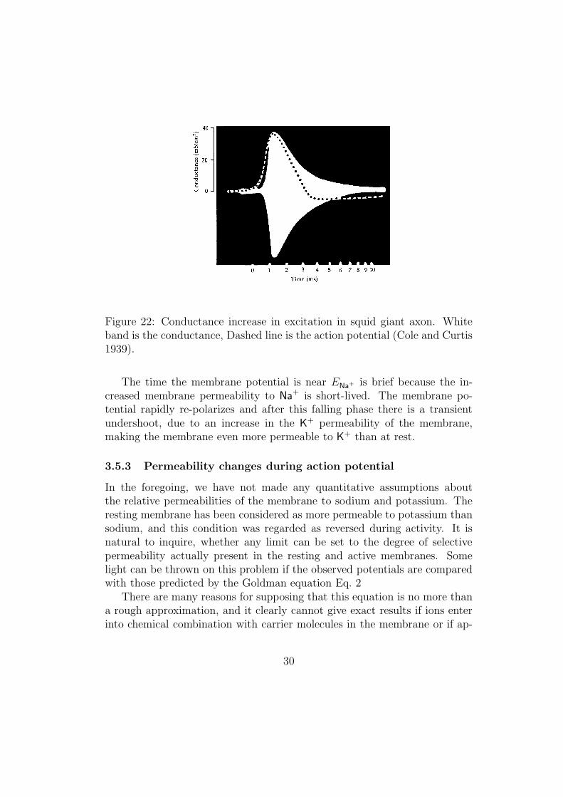
Figure 22: Conductance increase in excitation in squid giant axon. Whiteband is the conductance, Dashed line is the action potential (Cole and Curtis1939).

The time the membrane potential is near ENa+ is brief because the in-creased membrane permeability to Na+ is short-lived. The membrane po-tential rapidly re-polarizes and after this falling phase there is a transientundershoot, due to an increase in the K+ permeability of the membrane,making the membrane even more permeable to K+ than at rest.

3.5.3 Permeability changes during action potential

In the foregoing, we have not made any quantitative assumptions aboutthe relative permeabilities of the membrane to sodium and potassium. Theresting membrane has been considered as more permeable to potassium thansodium, and this condition was regarded as reversed during activity. It isnatural to inquire, whether any limit can be set to the degree of selectivepermeability actually present in the resting and active membranes. Somelight can be thrown on this problem if the observed potentials are comparedwith those predicted by the Goldman equation Eq. 2

There are many reasons for supposing that this equation is no more thana rough approximation, and it clearly cannot give exact results if ions enterinto chemical combination with carrier molecules in the membrane or if ap-

30

preciable quantities of current are transported by ions other K+, Na+ or Cl−.But because of its simplicity, and because it reduces to the correct Nernstequation if only one of the ion permeabilities dominates, Hodgkin and Katzused it anyway.

In the physiological condition of the axon that they used, the internal ionconcentrations were the following:

[K+]i = 345mM, [Na+]i = 72mM, [Cl−]i = 61mM

The experimental data against which the Goldman equation was tested aresummarized in Table 2, which shows the average change in membrane poten-tial produced by considering various external ion concentrations. It is seen,that there is reasonable agreement between all the results obtained with rest-ing nerve and those predicted by the theory for P+

K : P+Na : P−Cl = 1 : 0.04 :

0.45. These coefficients were obtained by trial and error. The value of theresting potential predicted on the basis of these values is 59 mV, while theobserved resting potential averaged 48 mV. The difference is due to a liquidjunction potential of 11 mV between sea water and axoplasm.

The peak of the action potential can be calculated if values are assumedfor the relative permeabilities of the active membrane to sodium, potassiumand chloride ions: with P+

K : P+Na : P−Cl = 1 : 20 : 0.45 an action potential

of -49 mV is obtained, which is roughly in agreement with the experimentalvalue -40 mV. These values of the permeabilities may be used to predict thechanges in potential when the external ion concentrations are changed insolutions A-I and are in reasonable agreement with the observed values.

The third block of numbers in Table 2 gives the changes in membranepotential recorded during the hyper-polarization of the action potential. Inthis condition the nerve is in a refractory state. Hodgkin and Katz assumedthat the sodium permeability is reduced to zero and that it does not recoverits normal value until the end of the relative refractory period. Using P+

K :P+

Na : P−Cl = 1.8 : 0 : 0.45 give good agreement between the Goldman equationand the observed values.

31

Table 2: (From [2]) showing the change in membrane potential when the exter-

nal concentrations of potassium, sodium and chlorine are changed under three

conditions: at rest, during the peak of the action potential, and after the action

potential. In each of these three conditions, the relative permeabilities of the three

ions are adjusted to obtain agreement between the experimental results and those

obtained by the Goldman equation Eq. 2. It shows that Ca2+ permeability is

highly increased during the action potential. Note, that Hodgkin and Katz used

a definition of the membrane potential that is minus the modern definition used

throughout this reader.32

3.6 Summary

The resting membrane potential is the result of different ions concentrationsinside and outside the cell and the specific permeability of the membraneto different ions. The relation between ionic concentrations and equilibriummembrane potential is described by the Nernst equation for single ions and bythe Goldman equation for multiple ions. At rest, the nerve cell is mainly per-meable to K+ ions resulting in a negative resting membrane potential. Duringthe action potential, the Na+ permeability dominates and the membrane po-tential reverses sign. The increased Na+ permeability is short, resulting ina short voltage spike. After the action potential, the Na+ permeability isreduced to zero, leading to a hyper-polarization of the membrane. Duringthis so-called refractory period no new action potentials can be generated.

Although we have identified the ions that flow during an action potential,we did not establish how the membrane is able to change the ionic permeabil-ity. As we will see in the next chapter, it is the neural membrane potentialitself that affects the membrane permeability.

The discussion of the ion channels, Nernst equation and Goldman equa-tion is based on [1]. The derivation of the Nernst-Planck and Goldmanequations and the description of the Hodgkin-Katz experiment is from [2].

3.7 Exercises

1. Explain why in Fig. 18, all excess charge accumulates near the mem-brane on both sides.

2. Consider the membrane of a neuron as a capacitor that can hold anamount of charge proportional to the potential difference: Q = CV .V is the potential difference between outside and inside of the cell andis measured in Volt, Q the charge on either side of the membrane andis measured in Coulomb per cm2 (C/cm2) and C is the capacitancemeasured in Farad per cm2 (F/cm2).

(a) Compute the capacitance, approximating the membrane by a par-allel plate capacitor:

C =εε0A

d

ε0 is the polarizability of free space and is 8.85× 10−12CV −1m−1.The dielectric constant of hydrocarbon chains is ε = 2.1. The

33

thickness of the membrane is 2.3 nm.

(b) Compute the number of charged ions that are required to maintainthe Nernst potential at 58 mV.

3. (a) What would happen to the Nernst potential if in the experimentof fig. 18 the K+ ions were replace by Na+?

(b) What would happen to the Nernst potential if in the experimentof fig. 18 the K+ ions were replace by Ca2+ and the membranewould be selectively permeable for Ca2+?

(c) What would happen to the Nernst potential if in the experiment offig. 18 the K+ ions were replace by Cl− and the membrane wouldbe selectively permeable for Cl−?

4. (a) Solve the Nernst-Planck Eq. 4 for constant Ii under the boundaryconditions Eq. 3 and assuming that the electrical potential changeslinearly with x within the membrane: V (x) = V x/a. Derive Eq. 5.

(b) Show the rectification behavior of Eq. 5 by computing its behaviorfor large positive and negative V .

5. Derive the Goldman equation Eq. 2 for the case most relevant to neu-rons, in which K+, Na+ and Cl− are the primary permeant ions. Usethe current voltage relations Eq. 5 and the additional condition thatno net charge is flowing,

∑i Ii = 0,

6. Explain the deviation between the experimental curve in fig. 20 and thetheoretical prediction by the Nernst equation in terms of the Goldmanequation Eq. 2

7. (a) Derive Eq. 7 from Eq. 6

(b) Show that the conductance increases when ion concentrations in-crease. Explain this effect in words.

8. The Nernst-Planck equations Eq. 5 and 6 relate the current to mem-brane voltage and ion concentrations. In this exercise, we compareexperimental values with those found by Eq. 5 and 6.

(a) Some experimental measurement on the squid axon in rest showsan average increase of the intracellular Na+ of 50 mM and an av-erage decrease of the intracellular K+ of 72 mM during a period of

34

3 hours. Express these findings in flow of ions per second througha surface of 1 cm2, assuming a cylindrical axon with diameter of500 µm.

(b) Eq. 5 gives the individual currents in terms of the experimentallyaccessible quantities: the ion concentrations and the membranepotential. The unknown quantity is the ion mobility ui. Use theequation for the conductivity in the Goldman equilibrium Eq. 7 towrite Eq. 5 for K+ and Na+ such that it involves only permeabilityratios of the various ions and the membrane conductance G.

(c) Compute the theoretical value for IK+ and INa+ given the followingvalues. The internal ion concentrations are [K+]in = 345mM, [Na+]in =72mM, [Cl−]in = 61mM . The external ion concentrations are[K+]out = 10mM, [Na+]out = 455mM, [Cl−]out = 540mM . Thepermeability ratios when the membrane is at rest are u+

K : u+Na :

u−Cl = 1 : 0.04 : 0.45. The temperature is 200C (RTF

= 25.26mV )and membrane resistance is 1000 Ω cm2.

35

4 The Hodgkin-Huxley model of action po-

tentials

4.1 The voltage clamp technique

This technique was invented by Kenneth Cole in 1940s. The device is calleda voltage clamp because it controls, or clamps, membrane potential at anylevel desired by the experimenter (see fig. 23). This electronic feedback circuitholds the membrane potential at the desired level, even in the face of per-meability changes that would normally alter the membrane potential. Also,the device permits the simultaneous measurement of the current needed tokeep the cell at a given voltage. Therefore, the voltage clamp technique canindicate how the membrane potential influences ionic current flow across themembrane. The most popular contemporary version of the voltage clamp isthe patch clamp technique (fig. 23E), which has a resolution high enough tomeasure the minute electrical currents flowing through a single inn channel(fig. 17)

4.2 Two types of voltage dependent ionic currents

In the late 1940s, Alan Hodgkin and Andrew Huxley used the voltage clamptechnique to work out the permeability changes underlying the action po-tential. They chose to use the giant neuron of the squid because its largesize (up to 1 mm in diameter) allowed insertion of the electrodes necessaryfor voltage clamping. To investigate the voltage dependent permeability ofthe membrane they asked whether ionic currents flow across the membranewhen its potential is changed. Fig. 24A illustrates the currents produced by asquid axon when its membrane potential is hyper-polarized from the restinglevel of -65 mV to -130 mV. The initial response of the axon results fromthe redistribution of charge across the membrane. This capacitive current isnearly instantaneous, ending within a fraction of a millisecond. Aside fromthis event, very little current flows when the membrane is hyper-polarized.However, when the membrane potential is depolarized from -65 mV to 0 mV,the response is quite different (fig. 24B). The axon produces a rapidly risinginward ionic current, which later changes into an outward current. This com-plicated relation between voltage and current suggests that the membranepermeability is indeed voltage dependent (exercise).

36

Figure 23: 1) One internal electrode measures membrane potential and isconnected to the voltage clamp amplifier. 2) Amplifier compares membranepotential to the desired potential. 3) When different, the amplifier injectscurrent into the axon through a second electrode, and is measured (4).

37

Figure 24: Current flow across a squid axon membrane during a voltageclamp experiment. A) A 65 mV hyper-polarization produces only a briefcapacitive current. B) A 65 mV depolarization produces in addition a longerlasting current that initially flows inward and later flows outward [3].

38

Figure 25: A squid giant axon membrane is stepped under voltage clampfrom a holding potential of -60 mV to potentials ranging in 20 mV stepsfrom -10 to +90 mV. Successive current traces have been superimposed [3].

Fig. 25 shows how the transient inward current and the sustained outwardcurrent depend on the clamp potential. Increasing the clamp potential fromthe resting value first shows an increase in the magnitude of the inwardcurrent up to approximately 0 mV, but this current decreases as the potentialis depolarized further. In contrast, the late current increases monotonicallywith increasingly positive membrane potentials.

These different responses to membrane potential can be seen more clearlywhen the magnitudes of the two current components are plotted as a functionof membrane potential (fig. 26). Note, that the early inward current becomeszero when the membrane is clamped at +52 mV. For the squid axon studiedby Hodgkin and Huxley, the external Na+ concentration is 440 mM and theinternal Na+ concentration is 50 mM. The corresponding Nernst potentialfor Na+ (see section 3.2) is computed as +55 mV. This equilibrium potentialis by definition the potential at which there is no net Na+ current acrossthe membrane. The proximity of these two values suggests that the inwardtransient current is caused by Na+ ions.

39

Figure 26: Relationship between current amplitude and membrane potential,taken form experiment such as in fig. 25. Whereas the late outward currentincreases steeply with increasing depolarization, the early inward current firstincreases in magnitude, but then decreases and reverses to outward currentat about +50 mV [3].

40

Figure 27: Dependence of the early inward current on sodium. In the pres-ence of a normal external concentration of Na+, depolarization of a squidaxon to -9 mV produces an inward initial current. However, reduction of theexternal Na+ removes the early inward current. The external Na+ concen-tration does not affect the late outward current [4].

An even more compelling way to test whether Na+ carries the early inwardcurrent is to examine the behavior of this current after reducing the externalNa+ concentration by a factor of 10. In this case, both internal and externalNa+ concentrations are approximately equal and the Na+ Nernst potential isclose to 0 mV. In fig. 27, we see indeed that under this condition a voltagestep to -9 mV does not evoke the early transient current, in agreement withthe Na+ hypothesis. Notice also that the reduction of external Na+ has noeffect on the outward current. This shows that the late outward currentmust be due to the flow of an ion other than Na+. Several lines of evidencepresented by Hodgkin, Huxley ad others showed that this late current iscaused by K+ exiting the neuron. Modern evidence that there are distinctmechanisms for Na+ and K+ come from pharmacological studies using drugsthat specifically affect these two currents (fig. 28).

Hodgkin and Huxley used a simple relation between current and voltagesuch as eq. 8 to calculate the dependence of the conductance on voltage:

Ii = gi(V, t)(V − Vi), i = K+,Na+ (9)

with Vi the reversal potential for ion i, V the membrane potential and Ii

41

Figure 28: Pharmacological separation of Na+ and K+ currents. Panel 1shows the current that flows when the membrane potential of a squid axon isdepolarized to -10 mV in control conditions. 2) Treatment with tetrodotoxincauses the early Na+ currents to disappear but spare the late K+ currents. 3)Addition of tetraethyl-ammonium blocks the K+ currents without affectingthe Na+ currents [5, 6].

42

the ion current. Some examples of the current voltage relations are givenin fig. 29. A and B show the passive case, where the conductance doesnot depend on voltage nor time, for different gi and Vi. C and D show whatshapes can occur when the conductance is voltage dependent but independentof time. Note the similarity in shape between figs. 29E and 26.

From fig. 26 and eq. 9 and from the known reversal potentials Vi onecan compute the conductance gi(V ) as a function of voltage. The result isshown in fig. 30. Hodgkin and Huxley concluded that both conductances arevoltage dependent and increase sharply when the membrane is depolarized.

In addition, Hodgkin and Huxley showed that the conductances changeover time. For example, both Na+ and K+ conductances require some time toactivate. In particular, the K+ conductance has a pronounced delay, requiringseveral milliseconds to reach its maximum (see fig. 31). The more rapidactivation of the Na+ conductance allows the resulting inward Na+ currentto precede the delayed outward K+ current. The Na+ current quickly declineseven though the membrane potential is kept at a depolarized level. This factshows that depolarization not only causes the Na+ conductance to activate,but also cause it to decrease over time, or inactivate. The K+ conductance ofthe squid axon does not inactivate in this way. Thus, while Na+ and K+ bothshow time dependent activation, only the Na+ conductance in-activates. Thetime course of the Na+ and K+ conductances are also voltage dependent, withthe speed of both activation and inactivation increasing at more depolarizedpotentials.

4.3 The Hodgkin-Huxley model

Hodgkin and Huxley’s goal was to account for ionic fluxes and permeabilitychanges in terms of molecular mechanisms. However, after intensive consid-eration of different mechanisms, they reluctantly concluded that still moreneeded to be known before a unique mechanism could be proven. Instead,they determined an empirical kinetic description that would be sufficientlygood to predict correctly the major features of excitability. This is called theHodgkin Huxley (HH) model.

The HH model is given in fig. 32. It consists of the Na+ and K+ cur-rents, a capacitative term and a leakage term. The Na+ and K+ currentsare each described by eq. 9. These currents are zero when the membranepotential is equal to their respective reversal potentials Vi, i = Na+,K+. Theconductances of these currents are both voltage and time dependent as we

43

Figure 29: A) Conductance increases when more channels are open; B)Nernst or reversal potential differs for different ions or same ion in differ-ent bathing solutions; C-D) Conductance is voltage dependent.

44

Figure 30: Depolarization increases Na+ and K+ conductances of the squidgiant axon. The peak magnitude of Na+ conductance and steady-state valueof K+ conductance both increase steeply as the membrane potential is depo-larized [7].

45

Figure 31: Membrane conductance changes underlying the action potentialare time- and voltage-dependent. Both peak Na+ and K+ conductances in-crease as the membrane potential becomes more positive. In addition, theactivation of both conductances occur more rapidly with larger depolariza-tions [7].

46

Figure 32: The Hodgkin Huxley model for the squid giant axon describes themembrane as an electrical circuit with four parallel branches.

will describe shortly.The leakage term is of the similar form eq. 9 but with a passive con-

ductance (time-independent and voltage independent). The leakage reversalpotential is empirically determined to be close to 0 mV 1

In addition, there is a capacitative branch. As we discuss in exercise1, the concentration difference of the ions results in a charge build-up withopposite charge on either side of the membrane. To lowest order, the chargeis proportional to the potential difference:

Q = CV

with Q the charge in Coulomb per unit area and C the capacitance. Becausethe membrane is so thin (a ≈ 2 nm), we can safely treat the membrane as

1The leakage conductance is the inverse of the resistance. The resistance is proportionalto the thickness of the membrane. Also, the resistance of a sheet of membrane will decreasewhen we consider a larger area. Thus, we define the resistivity ρ as a property of themembrane material so that the resistance of a membrane of thickness a and area A is

R =ρa

A.

47

two parallel planes, separated by a distance a. Then the capacitance is givenby

C =εε0A

d(10)

For hydrocarbon ε ≈ 2, this results in a very high specific capacitance of≈ 1µF/cm2. The current through the capacitor is

Ic = CdV

dt, (11)

where V is the membrane potential relative to the resting potential Vrest.We will now model the time and voltage dependence of the K+ and Na+

currents. Because it is simpler, we first consider the K+ conductance.

4.3.1 The K+ conductance

The time and voltage dependence of gK+ is empirically given in fig. 31. HHproposed to write the conductance as

g+K = gK+n4 (12)

with gK+ the maximal conductance when all K+ channels are open. n is adynamic quantity and its differential equation is given by

τn(V )dn

dt= n∞(V )− n (13)

τn and n∞ are the characteristic time constant for change in n and its station-ary value, respectively. Both are voltage dependent (but time independent),as we see from fig. 31. The detailed dependence of τn and n∞ on the mem-brane potential is given in fig. 33.

The response of eqs. 12 and 13 to a depolarizing voltage step is shownin fig. 34. It is seen, that the exponent 4 ensures that the K+ conductanceincreases with slope zero in agreement with experiment. Instead, if gK+ wereproportional to n it would increase with non-zero slope. The exponent 4 wasfound at the time to give the best numerical fit. It was hypothesized by HHthat the K+ channel is controlled by four independent gates. All gates mustbe open for the channel to be open. If n denotes the probability that one ofthe gates is open, this reasoning explains the exponent 4 in eq. 12.

48

Figure 33: Dependence of the characteristic time constants τm,h,n and steadystate values m∞, h∞ and n∞ on the squid axon membrane potential. Thesevalues produce the solid lines in fig. 31.

Figure 34: Response of n, h and m to a depolarizing and re-polarizing po-tential.

49

Figure 35: Inactivation of sodium current. A) Sodium currents elicited bytest pulses to -15 mV after 50 milliseconds pre-pulses to three different levels.The current is decreased by depolarizing pre-pulses. B) The relative peak sizeof the sodium current versus the pre-pulse potential, forming the steady stateinactivation curve of the HH model. Bell-shaped curve shows the voltagedependence of the exponential time constant of the inactivation process.

4.3.2 The Na+ conductance

The Na+ conductance is more complicated than the K+ conductance, be-cause there are independent activation and inactivation processes at work.The effect of Na+ inactivation is shown in fig. 35. In this experiment, thedependence of the Na+ current on the resting potential before the voltagestep is shown. The membrane potential is first clamped to -60, -67.5 or -75mV for 50 milliseconds. Subsequently, the membrane potential is raised to-15 mV. The figure shows that the peak value of the resulting Na+ currentdecreases with increasing pre-step membrane potential. The explanation ofthis phenomenon is the Na+ inactivation. As a result of the pre-step clamp-ing, the voltage dependent Na+ inactivation will settle to different values.The equilibrium inactivation 1 − h∞ is an increasing function of the mem-brane potential: For hyper-polarized membrane potential, inactivation is zero(h∞ = 1) and activation of the channel yields the largest current. For a par-

50

tially depolarized membrane potential, the inactivation settles to a non-zerovalue and thus h∞ < 1.

Hodgkin and Huxley postulated that the Na+ conductance is given by

gNa+ = gNa+m3h (14)

with gNa+ the maximal conductance when all Na+ channels are open. m andh are dynamic quantities similar to n. Their differential equation is given by

τm(V )dm

dt= m∞(V )−m (15)

τh(V )dh

dt= h∞(V )− h (16)

τm,h are the characteristic time constants for change in m and h, respectively.m∞ and h∞ are their stationary values. All are voltage dependent, as we seefrom fig. 33.

For the resting membrane, the activation variable m∞ and the inactiva-tion variable 1− h∞ are close to zero. During a spike, m increases from zeroto one, while h decreases from 1 to zero. As a result, the product m3h showsa peak with a shape similar to the early transient Na+ current (fig. 34).

4.3.3 Action potentials

We can now summarize the Hodgkin Huxley model. From fig. 32 we have

Ic + INa+ + IK+ + Ileak + Iext = 0

where we have added an external current, that we can use to provide currentinput to the cell. Combining eqs. 9-16, we obtain

CdV

dt= −m3hgNa+(V − VNa+)− n4gK+(V − VK+)

−gleak(V − Vleak)− Iext(t)

τndn

dt= n∞ − n

τmdm

dt= m∞ −m

τhdh

dt= h∞ − h (17)

51

Figure 36: A) The solution of the Hodgkin-Huxley eqs. 17 for the membranepotential V and the conductances gK+n4 and gNa+m3h as a function of time.Membrane depolarization rapidly opens Na+ channels, causing an inrush ofNa+ ions, which in turn further depolarized the membrane potential. Slowerinactivation of Na+ and activation of K+ channels restores the membranepotential to its resting value. B) Local current flows associated with propa-gation. Inward current at the excited region spreads forward inside the axonto bring the unexcited regions above the firing threshold.

where Vi and gi, i = K+,Na+, leak are constants and τn,m,h and n∞, m∞and h∞ are voltage dependent as given in fig. 33. Thus, the HH equationsconstitute a coupled set of 4 non-linear first order differential equations.

The HH equations were developed to describe the voltage and time de-pendence of the K+ and Na+ conductances in a voltage clamp experiment.However, they can in fact also generate the form and time course of the ac-tion potential with remarkable accuracy (fig. 36). The initial depolarizationof the membrane is due to the stimulus. This increases the Na+ permeability,which yields a large inward Na+ current, further depolarizing the membrane,which approaches the the Na+ Nernst potential VNa+. The rate of depolar-ization subsequently falls both because the electrochemical driving force on

52

Na+ decreases and because the Na+ conductance in-activates. At the sametime, depolarization slowly activates the K+ conductance, causing K+ ions toleave the cell and re-polarizing the membrane potential toward VK+. Becausethe K+ conductance becomes temporarily higher than it is in the resting con-dition, the membrane potential actually becomes briefly more negative thanthe normal resting potential (the undershoot). The hyper-polarization ofthe membrane potential causes the voltage-dependent K+ conductance (andany Na+ conductance not in-activated) to turn off, allowing the membranepotential to return to its resting level.

4.4 Spike propagation

The voltage dependent mechanisms of action potential generation also ex-plains the long-distance transmission of these electrical signals. This trans-mission forms the basis of information processing between neurons in thebrain. Table 37 shows some conduction velocities for different types of nervefibers. As we see, thick axons and myelinated fibers conduct much faster thanthin and unmyelinated fibers, as we will explain below. Spike propagation isan active process, more like burning a fuse than electrical signaling in a cop-per wire. The latter is impossible because the axon longitudinal resistanceis exceedingly high due to its small diameter. Therefore, one needs repeatedamplification along the axon, which is what the spikes do. However, we firstdiscuss passive current flow.

4.4.1 Passive current flow

Current conduction by wires, and by neurons in the absence of action poten-tials, is called passive current flow. It plays a central role in action potentialpropagation, synaptic transmission and all other forms of electrical signalingin nerve cells. For the case of a cylindrical axon, such as the one depictedin Fig. 38, subthreshold current injected into one part of the axon spreadspassively along the axon until the current is dissipated by leakage out acrossthe axon membrane.

Radial currents (through the membrane) as well as axial currents (alongthe axon axis) result from ion movement, which is due to the electric field aswell as due to diffusion. We assume that we can safely ignore the contributiondue to diffusion, ie. Ohms law is valid (see discussion of the Nernst-Planckequation in section 3.4). The axial current is much larger than the radial

53

Figure 37: Neural information processing depends on spike propagation fromone cell to the next. The action potential lasts about 1 µsec and travels at1-100 m/sec.

54

Figure 38: Linear cable model models the passive electrical properties of theaxon.

current due to the fact that the membrane resistance is much higher thanthe intracellular resistance. Due to the small extracellular resistance, theexternal potential differences are small. Therefore, we assume a constantexternal potential independent of space and time.

As we will derive in exercise 5, the membrane potential, axial and ra-dial membrane currents satisfies the following partial differential equations,known as the cable equation2:

λ2∂2V

∂x2= τm

∂V

∂t+ V − rmiinj

∂V

∂x(x, t) = −raIi(x, t)

im(x, t) = −∂Ii∂x

(x, t) (18)

with V = Vi−Vrest the internal membrane potential with respect to the mem-brane resting potential; Ii is the axial current; ra∆x is the axial resistance ofa cylinder of length ∆x; im(x, t)∆x is the radial membrane current through

2These equations played an important role in the early 20th century for computing thetransmission properties of transatlantic telephone cables.

55

a ring of thickness ∆x; rm/∆x is its resistance and cm∆x is it capacitance.λ2 = rm/ra and τm = rmcm the space and time constants.

Suppose, a constant current is injected at x = 0. The membrane potentialreaches the steady-state solution satisfying

λ2d2V (x)

dx2= V (x)− rmiinj(x)

iinj(x) = I0δ(x)

The solution is given by

V (x) = V0 exp(−|x|/λ)

We can compute V0 by observing that dVdx x=0

= −V0

λ= −raIi(x = 0) = raI0

2

or

V0 =raI0λ

2=

√rarm2

I0

The membrane potential decreases with distance following a simple exponen-

tial decay, with characteristic length scale λ =√rm/ra. Hence, to improve

the passive flow of current along an axon, the resistance of the membraneshould be as high as possible and the resistance of the axoplasm should below.

Due to the membrane capacitance, there is a time delay of the membranepotential response to a chance in the input current. As a simplest example,consider the case that the potential is independent of location. If at t = 0the injected current is changed from zero to a constant value I, the voltageresponse is easily computed from eq. 18:

V (t) = V∞(1− exp(−t/τm))

with V∞ = Irm. We see that V (t) changes with the characteristic timeconstant τm = rmcm. In general, with more complex geometries than thecylindric axon and a membrane potential that changes with x, the timecourse of the change in membrane potential is not simply exponential, butnonetheless depends on the membrane time constant.

We can easily get a rough idea of the conduction velocity in the passivecable as a function of the axon diameter d. First note, that since rm/∆xis the resistance through a ring of diameter d in radial direction, rm ∝ d−1.

56

Secondly, since ra∆x is the resistance through a ring of diameter d in axialdirection, ra ∝ d−2. Thus, the characteristic length scale λ depends on thediameter as

λ =

√rmra∝√d

The capacitance of the ring is cm∆x. Approximating the membrane as twoparallel plates, the capacitance is proportional to the area of the ring: cm ∝ d.Thus, the characteristic time scale τm depends on the diameter as

τm = rmcm ∝ d−1d = constant

We therefore estimate that the propagation velocity depends on the diameterof the axon as

v ∝√d (19)

This requires very thick axons for fast propagation (eg. squid giant axon).From the examples of unmyelinated axons from table 37 we see indeed thatthey approximately follow this square root law. Fig. 39 summarizes thepassive properties of the axon.

4.4.2 Spike propagation

If the experiment shown in Fig. 39 is repeated with a depolarizing currentpulse sufficiently large to produce an action potential, the result is dramat-ically different (Fig. 40). In this case, an action potential occurs withoutdecrement along the entire length of the axon, which may be a distance ofa meter or more. Thus, action potentials somehow circumvent the inherentleakiness of neurons.

How, then, do action potentials traverse great distances along such a poorpassive conductor? This is easy to grasp now we know how action potentialsare generated and how current passively flows along an axon (Fig. 41). Adepolarizing stimulus (synaptic input in in vivo situations or injected currentpulse in an experiment) locally depolarize the axon, thus opening the voltagesensitive Na+ channels in that region. The opening of Na+ channels causesan action potential at that site. Due to the potential difference between thatsite and neighboring sites, current will flow to neighboring sites (as in passiveconductance). This passive flow depolarizes the membrane potential in theadjacent region of the axon thus triggering an action potential in this region,and so forth. It is the active process of spike generation that boosts the

57

Figure 39: Passive current flow in an axon. A current passing electrode pro-duces a subthreshold change in membrane potential, which spreads passivelyalong the axon. With increasing distance from the site of current injection,the amplitude of the potential change is attenuated.

58

Figure 40: Propagation of a action potential. An electrode evokes an actionpotential by injecting a supra-threshold current. Potential response recordedat the positions indicated by micro-electrodes is not attenuated, but delayedin time.

59

signal at each site, thus ensuring the long-distance transmission of electricalsignals.

After the action potential has passed a site, the Na+ channels are in-activated and the K+ channels are activated for a brief time (the refractoryperiod) during which no spike can be generated. The refractoriness of themembrane in the wake of the action potential explains why action potentialsdo not propagate back toward the point of their initiation as they travel alongan axon.

4.4.3 Myelin

Fast information processing in the nervous system require fast propagation ofaction potentials. Because action potential propagation requires passive andactive flow of current, the rate of action potential propagation is determinedby both of these phenomena. One way of improving passive current flow isto increase the diameter of the axon as we saw in section 4.4.1. However,this requires very thick axons for fast conduction.

Another strategy to improve the passive flow is to insulate the axonalmembrane. For this reason, nerve fibers in vertebrates, except the smallest,are surrounded by a sheath of fatty material, known as myelin. The myelinsheath is interrupted at regular intervals, known as the nodes of Ranvier(Fig. 42). At these sites only, action potentials are generated. (If the en-tire surface of the axon were insulated, there would be no place for actionpotential generation.) An action potential generated at one node of Ranvierelicits current that flows passively within the myelinated segment until thenext node is reached. The local current then generates an action potentialin the next node of Ranvier and the cycle is repeated. Because action poten-tials are only generated at the nodes of Ranvier this type of propagation iscalled saltatory, meaning that the action potential jumps from node to node.As a result, the propagation speed of action potentials is greatly enhanced(Fig. 43).

This results in a marked increase in speed due to the increased speed ofthe passive conduction (see Exercise 6) and the time-consuming process ofaction potential generation occurs only at the nodes of Ranvier. Whereasunmyelinated axon conduction velocities range from about 0.5 to 10 m/s,myelinated axons can conduct at velocities up to 150 m/s.

Not surprisingly, loss of myelin, as occurs in disease such as multiplesclerosis, causes a variety of serious neurological problems.

60

Figure 41: Action potential conduction requires both active and passive cur-rent flow. Depolarization at one point along an axon opens Na+ channelslocally (Point 1) and produces an action potential at this point (A) of theaxon (time point t=1). The resulting inward current flows passively alongthe axon (2), depolarizing the adjacent region (Point B) of the axon. At alater time (t=2), the depolarization of the adjacent membrane has openedNa+ channels at point B, resulting in the initiation of the action potential atthis site and additional inward current that again spreads passively to an ad-jacent point (Point C) farther along the axon (3). This cycle continues alongthe full length of the axon (5). Note that as the action potential spreads, themembrane potential re-polarizes due to K+ channel opening and Na+ channelinactivation, leaving a ”wake” of refractoriness behind the action potentialthat prevents its backward propagation (4).

61

Figure 42: A) Diagram of a myelinated axon. B) Local current in responseto action potential initiation at a particular site flows locally, as describedin Fig. 41. However, the presence of myelin prevents the local current fromleaking across the internodal membrane; it therefore flows farther along theaxon than it would in the absence of myelin. Moreover, voltage-gated Na+

channels are present only at the nodes of Ranvier. This arrangement meansthat the generation of active Na+ currents need only occur at these unmyeli-nated regions. The result is a greatly enhanced velocity of action potentialconduction. Bottom) Time course of membrane potential changes at thepoints indicated.

62

Figure 43: Comparison of speed of action potential conduction in unmyeli-nated (upper) and myelinated (lower) axons.

63

Figure 44: Equivalent electrical model of a nerve cell. The rest membranepotential is represented by a battery Vrest. The resistance R = 1/G, with Gthe linearized approximation Eq. 7. The capacitance is given by Eq. 10.

4.5 Summary

Contemporary understanding of membrane permeability is based on evidenceobtained by the voltage clamp technique, which permits detailed characteri-zation of permeability changes as a function of membrane potential and time.For most types of axons, these changes consist of a rapid and transient risein the sodium permeability, followed by a slower but more sustained rise inthe potassium permeability. Both permeabilities are voltage-dependent, in-creasing as the membrane potential depolarizes. The kinetics and voltagedependence of Na+ and K+ permeabilities provide a complete explanation ofaction potential generation. A mathematical model that describes the be-havior of these permeabilities predicts virtually all of the observed propertiesof action potentials. The discussion of the voltage clamp method and theidentification of the K+ and Na+ currents is based on [1] and the originalpapers [4, 7]. The discussion of the Hodgkin-Huxley model is based on [8].

4.6 Exercises

1. Passive properties of the nerve cell. If we ignore the spike generationmechanism of the nerve cell, we can describe the electrical behavior byan equivalent linear electronic circuit, as shown in fig. 44. The currentthrough the resistor is equal to Ir = V/R and the current through the

64

Figure 45: An experiment showing the passive electrical properties of a cell.The cell is impaled with two intracellular electrodes. One of them passessteps of current. The other records the changes of membrane potential.

capacitance is given by C dVdt

, with the capacitance is given by Eq. 10.In addition, there may be an externally supplied current Iext.

Conservation of current implies

0 = Ic + Ir − Iext = CdV

dt+V

R− Iext τ

dV

dt= −V + IextR

with τ = RC the membrane time constant.

In the cell in fig. 45 one measures the voltage change as a function ofthe amount of injected current. Assume that the cell can be describedas an RC circuit

(a) At t < 0 the membrane potential is at rest and the current I(t) =0. Derive an expression for the membrane potential as a functionof time if for t > 0 the current has a constant value Iext(t) = I0.

(b) Estimate approximately from fig. 45 the resistance of the cell andthe RC time. Use these estimates to compute the surface area ofthe cell (assume the capacitance C = 1µF/cm2).

2. Consider the voltage clamp experiment in fig. 24. How would the cur-rent response be if the membrane permeability were not voltage depen-dent? Sketch the current response in fig. 24A and B.

65

3. Numerical simulation of the HH model in Matlab. For an introductionto Matlab see http://www.mines.utah.edu/gg_computer_seminar/

matlab/matlab.html?. Download the software of numerical simula-tion of the HH model from www.snn.kun.nl/~bert/biofysica/fcns/

spikes.zip. Unzip the file spikes.zip and go to the subdirectoryspikes. The program hh.m simulates the Hodgkin-Huxley equations.In this program, V − 60 denotes the membrane potential in mV. Theparameters αi and βi are related to the parameters τi, i = n,m, h andn∞, m∞ and h∞ in Eq. 17 as

τi =1

αi + βi, i = n,m, h

n∞ = αnτn

m∞ = αmτm

h∞ = αhτh

The program hh functions.m shows the dependence of these functionson membrane potential. By editing the program hh.m, we can studythe behavior of the neuron as we change several parameters.

Study how the spiking of the neuron depends on the external currentIext, by varying Iext. Make a table of the spike frequency of the neuronversus the external current for Iext = 0, 5, 10, 40, 200µA/cm2. What isthe minimal value of the current for repetitive spiking? What happensto the frequency and amplitude for large current values?

4. In this excersize we compare the electrical resistance of an axon wireto a copper wire.

(a) Compute the resistance of one meter of axon if the axon resistivityρ = 100Ωcm.

(b) To how many meters of copper wire does this correspond if onemeter of copper wire has a resistance of approximately 0.1 Ω?

5. Derive the cable equations 18 using Fig. 38.

6. Using a reasoning similar to that leading to eq. 19, derive an expressionfor the passive propagation velocity in myelinated axons as a functionof the membrane thickness and axon diameter.

66

5 Synapses

5.1 Introduction

The human brain contains at least 100 billion neurons, each with the abil-ity to influence many other cells. Clearly, highly sophisticated and efficientmechanisms are needed to enable communication among this astronomicalnumber of elements. Such communication is made possible by synapses,the functional contacts between neurons. Although there are many kindsof synapses within the brain, they can be divided into two general classes:electrical synapses and chemical synapses. Electrical synapses permit direct,passive flow of electrical current from one neuron to another. The currentflows through gap junctions, which are specialized membrane channels thatconnect the two cells. In contrast, chemical synapses enable cell-to-cell com-munication via the secretion of neurotransmitters: the chemicals released bythe presynaptic neurons produce change the electrical conductance of thepost-synaptic membrane by activating specific receptor molecules.

It is generally believed that the strength of chemical synapses can changethrough learning as a function of behavioral experience. Chemical synapseshave therefore received most attention in the study of how networks of neu-rons can realize biological function. However, recently it has become clearthat also electrical synapses may play an important role in neural informa-tion processing. In this chapter, however, we will restrict our attention tochemical synapses.

5.2 Chemical synapses

Chemical synapses come in a large variety and have a complex internal dy-namics. Synapses typically connect the axon of one cell to the dendrite ofanother cell, but dendro-dendritic synapses also occur. Autapses, an axonmaking connection onto its own dendritic tree, are rare on pyramidal cells,but occur more frequently on some classes of cortical inhibitory inter-neurons.

Synapses are small: about 0.5-1.0 µm in diameter and are densely packedin the brain. If their size is 1 µm, one mm3 full of synapses would contain109 synapses. In fact, the experimental estimate is very close to this: 8× 108

synapses/mm3 in mouse cortex. In addition, one mm3 of brain tissue contains100000 neurons, 4.1 km of axon (d ≈ 0.3µ) and 456 m of dendrite (d ≈ 0.9µ).Thus, the average neuron in the mouse cortex is connected to 8000 other

67

neurons and uses 4 mm of dendrite wire and 4 cm of axon wire to connect toother cells. Since the total cortical surface in humans is about 100000 mm2

and 2 mm thick, there are about 2× 1010 neurons and 2× 1014 synapses inthe human brain. Fig. 2 shows some examples of chemical synapses in adultcat visual cortex.

The space between the pre-and postsynaptic neurons is called the synap-tic cleft. The key feature of all chemical synapses is the presence of small(30-40 nm diameter), membrane-bounded organelles called synaptic vesicleswithin the presynaptic terminal. These vesicles are filled with one or moreneurotransmitters. These chemical agents act as messengers between thecommunicating neurons that gives this type of synapse its name.

Transmission at chemical synapses is based on an elaborate sequenceof events (Fig. 46). 1) Action potential causes an inrush of Ca2+ ions viavoltage dependent Ca channels. 2) Elevated Ca2+ concentration allows oneor more vesicles to fuse with the presynaptic neuron membrane, releasing itsneurotransmitter. 3) The neurotransmitter binds to postsynaptic receptors,increasing the permeability of post-synaptic ion channels. An in- or out-rushof current temporarily changes the post-synaptic potential (PSP).

5.3 The post-synaptic potential

Upon activation of a chemical synapse one can observe a rapid and transientchange in the postsynaptic potential. The response can be either excita-tory (EPSP) or inhibitory (IPSP). These EPSPs and IPSPs are caused byexcitatory and inhibitory post-synaptic currents (EPSCs and IPSCs).

The synaptic current rises fast and decays to zero in 20-30 msec. We seefrom Fig. 47 that the peak can be either positive or negative, depending onthe clamping potential. The peak current is linearly related to the membranepotential. This suggest that:

Isyn(t) = gsyn(t)(Vm − Vsyn)

The post-synaptic current is caused by a temporary increase in the membraneconductance, modeled by gsyn(t). Vsyn is the clamp voltage for which theresponse changes sign. Its value is synapse specific.

Electrical properties of a membrane with synapse can be very simplydescribed by an RC circuit as depicted in Fig. 48. Conservation of current

68

Figure 46: Canonical chemical synapse model. Action potential causes aninrush of Ca2+ ions via voltage dependent Ca channels. 2) Elevated Ca2+

concentration allows one or more vesicles to fuse with the presynaptic neuronmembrane, releasing its neurotransmitter. 3) The neurotransmitter bindsto postsynaptic receptors, increasing the permeability of post-synaptic ionchannels. An in- or out-rush of current temporarily changes the post-synapticpotential (PSP).

Figure 47: Activation of synapses made by the mossy fibers onto CA3 pyra-midal cells in the rodent hippocampus. A) The pyramidal cell is voltageclamped to different values and the clamp current is recorded.

69

Figure 48: Equivalent electrical circuit for fast voltage dependent chemicalsynapse.

gives

CdVmdt

+ gsyn(t)(Vm − Vsyn) +Vm − Vrest

R= 0

τdV

dt= − (1 +Rgsyn)V − Rgsyn (Vrest − Vsyn)

with V = Vm − Vrest and τ = RC.When Vsyn > Vrest the current will depolarize the membrane. An example

is the excitatory synapse using the neurotransmitter glutamate with Vsyn −Vrest=80mV. When Vsyn < Vrest the current will hyper-polarize the membrane.An example is the inhibitory synapse using the neurotransmitter GABAB

that lets K ions out of the cell with Vsyn − Vrest=-10-30mV. The situation isillustrated in Fig. 49

Shunting inhibition occurs when Vrest = Vsyn. There is no synaptic current,but such synapses reduce the effect of other synapses. Consider one shuntingsynapse and one excitatory synapse:

τdV

dt= − (1 +Rgsyn +Rgsh)V − Rgsyn (Vrest − Vsyn)

The term Rgsh reduces the peak response of V . An example is the GABAA

synapse that increases the conductance to Cl ions with a reversal potentialnear the resting potential of many cells.

The summation of EPSPs and IPSPs by a postsynaptic neuron permits aneuron to integrate the electrical information provided by all the inhibitoryand excitatory synapses acting on it at any moment. If the sum of all inputresults in a depolarization of sufficient amplitude to raise the membranepotential above threshold, then the postsynaptic cell will produce an actionpotential (Fig. 50).

70

Figure 49: Reversal potentials and threshold potentials determine postsynap-tic excitation and inhibition. A, C) If the reversal potential for a PSP (Erev)is more positive than the action potential threshold (-40 mV), the effect ofa transmitter is excitatory, and it generates an EPSP. B) If the reversal po-tential for a PSP is more negative than the action potential threshold, thetransmitter is inhibitory and generates IPSPs.

Figure 50: Summation of postsynaptic potentials

71

Figure 51: Histogram of 198 miniature EPSPs after presynaptic stimulationand 78 spontaneous EPSPs (inset).

5.4 Stochastic PSPs

Much of the evidence leading to the present understanding of chemical synap-tic transmission was obtained from experiments at the neuromuscular junc-tion. These synapses between spinal motor neurons and skeletal musclecells are simple, large, and peripherally located, making them particularlyamenable to experimental analysis [9].

Stimulation of the presynaptic motor neuron under normal conditionsleads to a post synaptic action potential and contraction of the muscle. How-ever, also in the absence of stimulation, one can observe post-synaptic EPSPs,so-called miniature EPSPs, that are the result of spontaneous neurotransmit-ter release. Measuring the size of these events shows that they are alwaysmore or less of the same magnitude (Fig. 51 inset). This suggests that theseEPSPs are the result of the release of a single vesicle of neurotransmitter.

To test this hypothesis, Katz measured the post synaptic potential re-sulting from presynaptic stimulation when the concentration of Ca2+ in theextracellular medium is strongly reduced. In that case, the post-synapticcell does not generate an action potential and a sub-threshold post synapticresponse is observed instead. The magnitude of the response differs fromtrial to trial and the response is displayed as a histogram in Fig. 51. It isseen that the responses are clustered around multiples of 0.4 mV, which isthe mean size of the spontaneous (’quantal’) release mentioned above. Thus,pre-synaptic stimulation can lead to the opening of zero, one, two or up tofive vesicles of neurotransmitter. On average m = 2.33 vesicles are released.

We can model this process by assuming that the junction has n release

72

k np(k) Observed

0 19 181 44 442 52 553 40 364 24 255 11 126 5 57 2 28 1 19 0 0

Table 3: Numerical comparison between observed quantal response ofsynapse in neuro-muscular junction and prediction from binomial distribu-tion. n = 198, m = 2.33.

sites (n is a few hundred for neuro-muscular junction), each having an in-dependent probability p of releasing a vesicle after pre-synaptic stimulation.p depends of course on the Ca2+ concentration. The probability that thesynapse releases k quanta is then given by the binomial distribution

p(n, k) =

(nk

)pk(1− p)n−k

m = 〈k〉 = np

σ2 =⟨k2⟩−m2 = np(1− p)

In the limit, p → 0, n → ∞ with m = pn constant, the binomial distri-bution can be approximated by the Poisson distribution

p(n, k)→ p(k) =mk

k!exp(−m)

and the number of events for each k is given by np(k). As is demonstratedin exercise 1, np(k) reproduces these experimental findings very well.

With m = 2.33, the expected results for each k are compared with theexperimentally observed results in Table 3 and we see that the agreement isexcellent.

m = 2.33 n due to low external Ca. In normal operation m = O(n).

73

Figure 52: Left. EPSC in CA 1 pyramidal cells. Only 3 out of 9 presynaptic

stimuli produce a response. In addition, the response is variable in strength.

Right. Rat visual cortex. 4 EPSPs resulting from identical stimulation.

Whereas the neuro-muscular junction has many hundreds of synapticcontact, in cortex one finds mostly mono-synaptic connections and 0.1 <p < 0.9. Thus, information transmission between individual neurons is noisyand unreliable, as is illustrated in fig. 52.

5.5 Learning

The earliest learning experiments are from the psychology literature. Firstthere is the phenomenon of habituation using Pavlov’s dog. In this exper-iment a bell rings (CS) and the dog turns her head (CR). After severalrepetitions, the dog stops paying attention to the bell. Thus, the same stim-ulus leads to a change in the response from ’head turn’ to ’no head turn’(fig. 53b).

Depending on the type of stimulus, habituation occurs or not. If thedog is show a piece of meat (US), the dog will salivate (UR). UR) on sightof meat (US). No matter how often the stimulus is presented, the dog willalways respond (fig. 53c).

74

Figure 53: Habituation experiments

75

Now, consider two stimuli CS (bell) and US (meat). By itself CS doesnot yield a response, but US does. Classical conditioning is the phenomenonthat when CS and US are presented together for some time, the dog willstart responding to CS alone.

This phenomenon can be explained by assuming a simple model thatcaptures the relation between stimuli and response:

R = Θ(JuSu + JcSc − θ)

Θ(x) is a threshold function that returns 1 for x > 0 and zero otherwise.R = 1, 0 denotes the response of the dog salivating or not, u = 1, 0 denotesthe presence of the unconditioned stimulus (meat) and c = 1, 0 denotesthe presence of the conditioned stimulus (bell). Ju and Jc are connectionsmodulating the dependence of R on u and c, respectively. If this model isoperational in the brain somewhere, Ju and Jc can be thought of as effectivesynaptic connections between neurons or groups of neurons.

Before the experiment the bell by itself does not yield a response, butthe meat does. Therefore: J c < θ and Ju > θ. After the experiment bothbell and meat yield the response. Therefore: J c > θ and Ju > θ. We canunderstand the change in Jc by the so-called Hebbian learning paradigm

∆J ∝ RS

76

The synaptic strength J is only increased when the post-synaptic responseR coincide with the pre-synaptic stimulus S. In the absence of the meatstimulus, the bell stimulus never yields a response R = 1 and therefore theconnection Jc between bell and salivate is not strengthened. When bothbell and meat are presented, the meat stimulus by itself will make the dogsalivate (R = 1). The Hebbian learning rule will then strengthen both theconnections Jc and Ju. When Jc grows in this way and exceeds θ, the dogwill start salivating when only the bell is presented. The strengthening of Juhas no effect since its value is larger than θ from the beginning.

5.6 Long term potentiation

Many synapses in the mammalian central nervous system exhibit long-lastingforms of synaptic plasticity that are plausible substrates for learning, memoryand permanent changes in behavior.

One experimentally observed pattern of synaptic activity is known aslong-term potentiation (LTP). LTP has been studied most in the hippocam-pus, an area of the brain that is especially important in the formation and/orretrieval of some forms of memory.

The progress in understanding LTP has relied heavily on in vitro studiesof slices of living hippocampus. The hippocampus contains several regions,the major ones being CA1 and CA3. Much of the work on LTP has focusedon the synaptic connections between the Schaffer collaterals (axons of CA3pyramidal cells) and and CA1 pyramidal cells. The experimental setup isillustrated in Fig. 54. A stimulus electrode can activate a Schaffer collateral.Single stimuli applied to a Schaffer collateral evokes EPSPs in the post-synaptic CA1 neuron. These stimuli alone do not elicit any change in synapticstrength. However, when the CAI neuron’s membrane potential is brieflydepolarized (by applying current pulses through the recording electrode) inconjunction with the Schaffer collateral stimuli, there is a persistent increasein the EPSPs, which can last for hours or days. LTP occurs not only at theexcitatory synapses of the hippocampus, but at many other synapses in avariety of brain regions, including the cortex, amygdala and cerebellum.

LTP is a specific strengthening of synaptic connection, without strength-ening other synapses that contact the same neuron (Fig. 55A). Another im-portant property is associativity (Fig. 55B). As noted, weak stimulation ofa pathway will not by itself trigger LTP. However, if one pathway is weaklyactivated at the same time that a neighboring pathway onto the same cell is

77

Figure 54: Pairing presynaptic and postsynaptic activity causes LTP.

strongly activated, both synaptic pathways undergo LTP. Note, that this isa cellular analog of the previously discussed mechanism for classical condi-tioning.

5.7 Hebbian learning

The simplest plasticity rule that follows the spirit of Hebb’s conjecture takesthe form

τwdw

dt= vu− λv (20)

where w is the synaptic strength, τw is a time constant that controls therate at which the weights change, and u and v are the neural activity of thepre- and post-synaptic cell, respectively. The first term on the right handside of Eq. 20 is the Hebbian term and increases the synapses proportionalto the product of pre- and post-synaptic activity. Hebbian plasticity is apositive-feedback process because effective synapses are strengthened, mak-ing them even more effective. This tends to increase post-synaptic firingrates excessively.

The second term is an effective way of controlling this instability anddecreases the synapse proportional to the total post-synaptic activity. λ isan adjustable constant. For one presynaptic neuron and one post-synapticneuron the net effect is that the synapse is increased (decreased) when thepre-synaptic activity u > λ (u < λ).

When u and v are changing with time, w will also change with timeaccording to Eq. 20. A nice simplification can be made when we assume that

78

Figure 55: A) Strong activity initiates LTP at active synapses without ini-tiating LTP at nearby inactive synapses. B) Weak stimulation of pathway2 alone does not trigger LTP. However, when the same weak stimulus topathway 2 is activated together with strong stimulation of pathway 1, bothsets of synapses are strengthened.

u and v are randomly drawn from a probability distribution p(u, v). In thiscase the average synaptic weight satisfies

τwdw

dt= 〈vu〉 − λ 〈v〉

with 〈uv〉 =∫dudvp(u, v)uv and 〈v〉 =

∫dudvp(u, v)v.

When a neuron receives input from n synapses with strength wi, thedeterministic rule becomes

τwdwidt

= vui − λv, i = 1, . . . , n (21)

Note, that the change of each synapse depends on the value of all othersynapses through v. For instance, if we assume that v depends linearly onthe inputs v =

∑ni=1 wiui.

5.7.1 Ocular dominance

Hebbian plasticity is often used to model the development and activity-dependent modification of neuronal selectivity to various aspects of a sen-sory input, for example the selectivity of visually responsive neurons to theorientation of a visual image. This typically requires competition betweensynapses, so that the neuron becomes unresponsive to some features while

79

growing more responsive to others. The above Hebbian rule Eq. 21 introducessuch competition, as we will show now.

We consider the highly simplified case of a single layer 4 neuron thatreceives input from just two LGN neurons with activity ui, i = 1, 2. Twosynaptic weights wi, i = 1, 2 describe the synaptic connection strengths ofthe LGN neurons with the cortical neuron. The output activity we assumesimply linear:

v =2∑

i=1

wiui (22)

Thus, Eq. 21 becomes

τwdwidt

=∑

j

Qijwj − λ(w1 〈u1〉+ w2 〈u2〉)

Qij = 〈uiuj〉 (23)

Using the symmetry property that both eyes are equal, we can parameterizethe matrix as Q11 = Q22 = qs, Q12 = Q21 = qd and 〈u1〉 = 〈u2〉 = 〈u〉.We can solve Eq. 23 by changing to the basis of eigenvectors of Q. Stateddifferently, the dynamical equations for w1 + w2 and w1 − w2 decouple:

τwd(w1 + w2)

dt= (qs + qd − 2λ 〈u〉)(w1 + w2) (24)

τwd(w1 − w2)

dt= (qs − qd)(w1 − w2) (25)

For λ sufficiently large, the first equation will yield the asymptotic solutionw1 + w2 = 0. Under normal circumstances, the cross correlation betweeneyes qd is smaller than the autocorrelation qs. Therefore, qs − qd > 0 andw1 − w2 will grow indefinitely. In reality, there will be non-linearities in thesystem (in Eq. 20 and Eq. 22) that will prevent this indefinite growth. Thefinal solution is then

w1 = −w2 = w∞ (26)

with w∞ a positive or negative value depending on the sign of the initialvalue w1(0)−w2(0). For w∞ > 0, the cortical neuron will be sensitive to eye1 and insensitive to eye 2, and vise versa. Thus, we have shown that oculardominance can explained as a consequence of Hebbian learning.

80

5.8 Summary

There are chemical and electrical synapses. Chemical synapses are thoughtto be implied in learning. Synapses can be excitatory, inhibitory or shuntingdepending on the reversal potential of the synapse relative to the membraneresting potential. Synapses are stochastic elements: a presynaptic action po-tential yields a postsynaptic response with a certain probability. The mostimportant mechanism for learning is called Hebbian learning. The strengthof a synapse increases when pre- and postsynaptic cell fire at the same time.This is in agreement with the psychological phenomenon of classical condi-tioning and also found as a mechanism for synaptic plasticity in the brain.Hebbian learning can be used to explain the receptive field properties ofmany neurons, such as for instance ocular dominance. This chapter is basedon [10, 1, 11].

5.9 Exercises

1. This exercize is about the quantal release of neurotransmitter at theneuro-muscular junction.

(a) Show that the binomial distribution reduces to the Poisson distri-bution in the limit p→ 0, n→∞ with m = pn constant.

(b) Check the numerical agreement between the Poisson distributionand the experimental values

(c) Discuss the shape of the distribution when the Ca2+ is restored toits normal physiological value. Compute the mean and varianceand explain why under these conditions the presynaptic spike givesa deterministic post-synaptic response.

81

Figure 56: A) Simple Perceptron B) Multi-layered Perceptron

6 Perceptrons

Perceptrons are feed-forward neural networks. Examples are given in Fig. 56.Consider a simple perceptron with one output:

o = g(h) = g

n∑

j=1

wjξj − θ = g

n∑

j=0

wjξj

with weights wj and inputs ξj. ξ0 = −1 and θ = w0. g is a non-linearfunction.

Learning: Given a number of input-output pairs (ξµj , ζµ), µ = 1, . . . , P ,

find wj such that the perceptron output o for each input pattern ξµ is equalto the desired output ζµ:

oµ = g

n∑

j=0

wjξµj

= ζµ, µ = 1, . . . , P

6.1 Threshold units

Consider the simplest case of binary threshold neurons:

g(h) = sign(h)

Then, the learning condition becomes

sign(w · ξµ) = ζµ, µ = 1, . . . , P

82

Since ζµ = ±1, we have

sign(w · ξµζµ) = 1 or w · xµ > 0

with xµj = ξµj ζµ.

6.2 Linear separation

Classification depends on sign of w · ξ. Thus, decision boundary is hyperplane:

0 = w · ξ =n∑

j=1

wjξj − θ

Perceptron can solve linearly separable problems. An example of a linearlyseparable problem is the AND problem: The output of the perceptron is 1 ifall inputs are 1, and -1 otherwise (see Fig. 57).

By definition, problems that are not linearly separable need more thanone separating hyper plane to separate the two classes. An example of anon-linearly separable problem is the XOR problem: The output is equalto the product of the input values (see Fig. 57A). Other problems that arenot linearly separable occur when three or more input patterns are linearlydependent (see Fig. 57B).

83

Figure 57: The AND problem for two inputs is linearly separable.

6.3 Perceptron learning rule

We have seen that the desired weight vector satisfies

w · xµ > 0, all patterns (27)

We define the following perceptron learning rule:

wnewj = wold

j + ∆wj

∆wj = ηΘ(−w · xµ)ξµj ζµ = ηΘ(−w · xµ)xµ (28)

η is the learning rate. This learning rule is Hebbian in the sense that thechange in weight is proportional to the product of input and output activity.

84

Figure 58: The perceptron learning rule in action. Learning rule Eq. 28is applied to all patterns in some random or given order. Learning stops,when a weight configuration is found that has positive inner product with alltraining patterns.

The function Θ is 1 for positive arguments and zero otherwise: When pre-senting pattern µ, learning only occurs, when the condition w · xµ > 0 is notsatisfied for that pattern.

In Fig. 58 we show the behavior of the perceptron learning rule withη = 1. The dataset consists of three data patterns x1, x2 and x3. Theinitial weight vector is w. Presenting pattern x1, we note that w · x1 < 0and therefore learning occurs. The resulting weight vector is w′ = w + x1.Presenting pattern x2 and x3 also result in learning steps and we end up inweight configuration w′′′. This weight vector has positive inner product withall training patterns and learning terminates.

Depending on the data, there may be many or few solutions to the learn-ing problem, or non at all! In Fig. 59 we give examples of two data sets andtheir solutions Eq. 27. In Fig. 59A there are more admissible weight vectorsand they can have a larger inner product with all training patterns than inFig. 59B. We define the quality of the solution w by the pattern that has thesmallest inner product with w. Since the solution does not depend on the

85

Figure 59: Two examples of data sets and the sets of w that satisfy conditionEq. 27. A) Many solutions B) Few solutions.

norm of w, we define the quality as

D(w) =1

‖w‖ minµw · xµ

The best solution is given by Dmax = maxwD(w).In Fig. 60, we illustrate this for a given data set and two admissible

solutions w and w′ and their values of D respectively. Since D(w′) > D(w),w′ is the preferred solution.

If we can find a w such that D(w) > 0 the problem is linearly separableand learnable by the perceptron learning rule. If the problem is not linearlyseparable not such solution exists.

6.3.1 Convergence of Perceptron rule

In this section we show that if the problem is linearly separable, the percep-tron learning rule converges in a finite number of steps. We start with initialvalue w = 0. At each iteration, w is updated only if w · xµ < 0. After somenumber of iterations, let Mµ denote the number of times pattern µ has beenused to update w. Thus,

w = η∑

µ

Mµxµ

M =∑µM

µ is the total number of iterations in which the weight vectoris updated. If the learning rule converges, it means that M is finite and doesnot grow indefinitely.

86

Figure 60: Two admissible solutions w and w′ and their values of D respec-tively. Since D(w′) > D(w), w′ is the preferred solution.

The proof goes as follows. Assume that the problem is linearly separable,so that there is a solution w∗ with D(w∗) > 0. We will show that

O(√M) ≤ w · w∗

‖w‖‖w∗‖ ≤ 1

where the second inequality follows simply from the definition of the innerproduct, and we will show the first inequality below. Thus, M can not growindefinitely and the perceptron learning rule converges in a finite number ofsteps.

The proof of the first inequality is elementary:

w · w∗ = η∑

µ

Mµxµ · w∗ ≥ ηM minµxµ · w∗ = ηMD(w∗)‖w∗‖

∆‖w‖2 = ‖w + ηxµ‖2 − ‖w‖2 = 2ηw · xµ + η2‖xµ‖2 ≤ η2‖xµ‖2 = η2N

The inequality in the second line makes use of the fact that for each trainingpattern where learning takes place w ·xµ < 0. The norm of w is thus boundedby

‖w‖2 ≤ η2NM

87

Combining these two inequality, we obtain Thus,

w · w∗|w||w∗| ≥

√MD(w∗)√

N(29)

which completes the proof. Note, that the proof makes essential use of theexistence of w∗ with D(w∗) > 0. If D(w∗) < 0 the bound Eq. 29 becomes atrivial statement and does not yield a bound on M .

If the problem is linearly separable, we can in conclude that the numberof weight updates:

M ≤ N

D2(w∗)

where N is some trivial constant. We see that convergence takes longer forharder problems (for which D(w∗) is closer to zero).

6.4 Linear units

We now turn to a possibly simpler case of linear units:

oµ =∑

j

wjξµj

Desired behavior is that the perceptron output equals the desired output forall patterns: oµ = ζµ, µ = 1, . . . , P . In this case, we can compute an explicitsolution for the weights. It is given by

wj =1

N

∑

ρν

ζρ(Q−1

)ρνξνj , Qρν =

1

N

∑

j

ξρj ξνj (30)

Q is a matrix with dimension P ×P and contains the inner products betweenthe input patterns.

To verify that Eq. 30 solves the linear perceptron problem, we simplycheck for one of the input patterns (ξµ) whether it gives the desired output:

∑

j

wjξµj =

1

N

∑

ρ,u,j

ζρ(Q−1

)ρνξuj ξ

µj

=∑

ρ,u

ζρ(Q−1

)ρνQνµ

=∑

ρ

ζρδρµ = ζµ

88

For this solution to exist, Q must be invertible. Therefore, the input pat-terns must be linearly independent. Because otherwise Q is not of maximalrank. Therefore, the number of patterns cannot exceed the number of inputdimensions: P ≤ N . 3

When P < N the solution wj = 1N

∑ρν ζ

ρ (Q−1)ρν ξuj is not unique. In

fact, there exists a linear space of dimension N − P of solutions w. Namely,let

w0j =

1

N

∑

ρν

ζρ(Q−1

)ρνξuj

wj = w0j + ξ⊥

with ξ⊥ an n-dimensional vector that is perpendicular to all training patterns:ξ⊥ ⊥ ξµ. Then the output of the perceptron is unaffected by ξ⊥:

ζµ =∑

j

wjξµj =

∑

j

(w0j + ξ⊥j )ξµj =

∑

j

w0j ξµj

6.4.1 Gradient descent learning

Often P > N , and thus patterns are linearly dependent. In general, one candefine a learning rules through a cost function, that assigns a cost or qualityto each possible weight vector. A common cost function is the quadratic cost:

E(w) =1

2

∑

µ

ζµ −

∑

j

wjξµj

2

3If the input patterns are linearly dependent, solution Eq. 30 does not exist. Lineardependence of the inputs implies that there exists αµ such that

∑

µ

αµξµj = 0

This implies that

∑

µ

αµζµ =∑

µj

wjαµξµj = 0

in other words, that the outputs cannot be chosen at freely. For problems with linearlydependent inputs and matched linearly dependent output Eq. 30 can be used by restrictingthe training set to a linearly independent subset that spans the training set, and computingQ for this subset.

89

which is minimized when the actual perceptron output∑j wjξ

µj is as close as

possible to the desired output ζµ for all patterns µ.The cost function can be minimized by the so-called gradient descent

procedure. We start with an initial random value of the weight vector w andwe compute the gradient in this point:

∂E

∂wi= −

∑

µ

ζµ −

∑

j

wjξµj

ξµi

We change w according to the ’learning rule’

wi = wi + ∆wi ∆wi = −η ∂E∂wi

(31)

and repeat this until the weights do not change any more.When η is sufficiently small, it is easy to verify that this gradient descent

procedure converges. The proof consists of two observations. One is thatfor small η, E(w) decreases in each step, and the other is that E(w) isbounded from below, so that it has a smallest value. Therefore E cannotcontinue decreasing indefinitely and must converge to some stationary value(see Exercises).

6.4.2 The value of η

What is a good value form η? Clearly, when η is very small, convergenceis guaranteed, but in practice it may take a very long time. If η is toolarge, however, convergence is no longer guaranteed. The problem is furthercomplicated by the fact that the optimal choice of η is different for differentcomponents of the weight vector w. This is illustrated in Fig. 61, where E asa function of w is drawn. This valley has a unique minimal value for E, butthe curvature in two directions is very different. In the long (flat) direction,large steps can be made, but in the orthogonal direction only small steps areallowed. We can analyze the problem, by assuming that the energy has theform

E(w) =1

2

∑

i

ai (wi − w∗i )2 + E0

with w∗ the location of the minimum, and ai the curvatures in the twodirections i = 1, 2. Eq. 31 becomes

∆wi = −η ∂E∂wi

= −2ηai (wi − w∗i ) = −2ηaiδwi

90

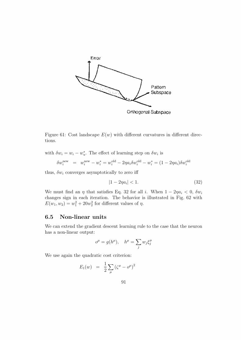
Figure 61: Cost landscape E(w) with different curvatures in different direc-tions.

with δwi = wi − w∗u. The effect of learning step on δwi is

δwnewi = wnew

i − w∗i = woldi − 2ηaiδw

oldi − w∗i = (1− 2ηai)δw

oldi

thus, δwi converges asymptotically to zero iff

|1− 2ηai| < 1. (32)

We must find an η that satisfies Eq. 32 for all i. When 1 − 2ηai < 0, δwichanges sign in each iteration. The behavior is illustrated in Fig. 62 withE(w1, w2) = w2

1 + 20w22 for different values of η.

6.5 Non-linear units

We can extend the gradient descent learning rule to the case that the neuronhas a non-linear output:

oµ = g(hµ), hµ =∑

j

wjξµj

We use again the quadratic cost criterion:

E1(w) =1

2

∑

µ

(ζµ − oµ)2

91

Figure 62: Behavior of the gradient descent learning rule Eq. 31for the quadratic cost function E(w1, w2) = w2

1 + 20w22 for η =

0.02, 0.0476, 0.049, 0.0505.

∆wi = −η ∂E∂wi

=∑

µ

(ζµ − oµ) g′(hµ)ξµi

When the function g is a monotonous function, it is invertible and onecould also formulate a different cost criterion by observing the identity

ζµ = g(hµ)⇔ g−1(ζµ) = hµ

E2(w) =1

2

∑

µ

(g−1(ζµ)− hµ

)2

Note, that E2 has a quadratic dependence on w, as in the linear case (butwith transformed targets g−1(ζµ) instead of ζµ). In general, optimizing eitherE1 or E2 yield different optimal solutions.

6.6 Multi-layered perceptrons

The gradient descent learning procedure can be trivially extended to theperceptron with multiple layers and multiple outputs as shown in Fig. 56B.In addition to the input variables ξk and the output variable oi, we have alayer of hidden variables vj for which no training data are observed. The

92

value of the hidden variables is computed in terms of the input variables,and the outputs are computed in terms of the hidden variables:

oi = g

∑

j

wijvj

= g

∑

j

wijg

(∑

k

wjkξk

) (33)

The output is now a complex function of the input pattern ξk and the weightswjk in the first layer of the network and the weights wij in the second layerof the network.

Given a set of P training patterns (ξµk , ζµi ), µ = 1, . . . , P , we again use

the gradient descent procedure to find the weights that minimize the totalquadratic error:

E(w) =1

2

∑

i

∑

µ

(oµi − ζµi )2

(34)

with oµi the output on node i for input pattern ξµ as given by Eq. 33.For large neural networks with many hidden units, the simple gradient

descent procedure can be quite slow. However, there exist well-known algo-rithms that significantly accelerate the convergence of the gradient descentprocedure. One such method is the conjugate gradient method. Treatmentof this method is beyond the scope of this course (see however [12] or Matlabfor further details).

Note, that the optimal solution that is found depends on the numberof hidden units in the network. The more hidden units, the more complexfunctions between input and output can be learned. So, for a given data set,we can make the error Eq. 34 as small as we like by increasing the numberof hidden units. In fact, one can show that the multi-layered perceptron canlearn any smooth function, given a sufficiently large number of hidden units.

However, the objective of a learning algorithm is to use the neural networkto predict the output on novel data, that were not previously seen. Increasingthe number of hidden units does not necessarily improve the prediction onnovel data. The situation is illustrated in Fig. 63 for the case of one inputvariable and one output variable. The crosses denote the data points thatwere used for training and the smooth curve is the neural network solution.For a small number of hidden units, the solution may look something likeFig. 63A. The solution does not pass through all the data points. For a largernumber of hidden units, the solution may look something like Fig. 63B.The solution does pass through all the data points and is more complex.However, the prediction of the more complex network is less accurate than

93

Figure 63: Network output versus network input. A) Network with a smallnumber of hidden units. B) Network with a large number of hidden units.Networks with more hidden units can implement more complex functionsand can better fit a given training set. However, more complex networks donot necessarily generalize better on novel data.

the simple network for the data point indicated by the circle, which was notpart of the training set. The extend to which the trained neural network iscapable of predicting on novel data is called the generalization performance.The network with the optimal generalization performance must balance twoopposing criteria: minimization of the error on the training data requiresa large number of hidden units, but the solution should also be sufficientlysmooth to give good prediction.

94

6.7 Summary

This chapter is based on [12]. Perceptrons are simple models of feed-forwardcomputation in a network of neurons. Binary perceptrons can be used forclassification problems. Learning is done using the perceptron learning rule.The learning rule converges in a finite number of iterations if and only if theproblem is linearly separable.

Perceptrons can also be constructed with continuous output, either usinga linear or non-linear transfer function. These perceptrons can be learned us-ing the gradient descent method. Gradient descent converges asymptoticallyfor any data set.

The quality of the perceptron can be significantly improved by usingmultiple layers of hidden units. The multi-layered perceptron can learn anyfunction by using a sufficiently large number of hidden units. However, pre-diction quality on novel data does not generally increase with the numberof hidden units. Optimal generalization is obtained for a finite number ofhidden units.

6.8 Exercises

1. Check dat Dmax = 1√3

voor het AND probleem en Dmax = − 1√3

voorhet XOR probleem. Het AND probleem in de ξi = ±1 codering isgedefinieerd als ζ = 1 als ξ1 = ξ2 = 1 and ζ = −1 in alle overigegevallen. Het XOR probleem is gedefinieerd als ζ = ξ1 ∗ ξ2. Gebruikvoor de gewichten vector w = (w0, w1, w2). (Hint: gebruik w1 = w2

vanwege symmetrie).

2. Beschouw gradient descent in een kostenlandschap gegeven door E =a1x

2 + a2y2. Bereken de leerparameter η zodanig dat de convergentie

in zowel x als y richting even snel is.

3. Beschouw een lineair perceptron (sectie 6.4) om de AND functie teleren.

• wat zijn de optimale gewichten en drempels? wat is de optimalekosten E?

• laat zien dat E > 0 impliceert dat de inputpatronen lineair afhanke-lijk zijn.

95

4. Toon aan dat het gradient descent algoritme Eq. 31 asymptotisch con-vergeert.

96

References

[1] D. Purves, G.J. Augustine, D. Fitzpatrick, L.C. Katz, A-S. LaMantia, andJ.O. McNamara. Neuroscience. Sinauer associates, 1997.

[2] A.L. Hodgkin and B. Katz. The effect of sodium ions on the electrical activityof the giant axon of the squid. Journal of Physiology, 108:37–77, 1949.

[3] A.L. Hodgkin, A.F. Huxley, and B. Katz. Measurements of current-voltagerelations in the membrane of the giant axon of loligo. Journal of Physiology,116:424–448, 1952.

[4] A.L. Hodgkin and A.F. Huxley. Currents carried by sodium and potassiumions through the membrane of a giant axon of loligo. Journal of Physiology,116:449–472, 1952.

[5] J.W. Moore, M.P. Blaustein, N.C. Anderson, and T. Narahashi. Basis oftetrodotoxin’s selectivity in blockage of squid axons. Journal of General Phys-iology, 50:1401–1411, 1967.

[6] C.M. Armstrong and L. Binstock. Anomalous rectification in the squid giantaxon injected with tetraethylammonium chloride. Journal of General Physi-ology, 48:859–872, 1965.

[7] A.L. Hodgkin and A.F. Huxley. The components of membrane conductancein the giant axon of loligo. Journal of Physiology, 116:473–496, 1952.

[8] B. Hille. Ionic Channels of excitable membranes. Sinaouer Associates, 1984.

[9] B. Katz. Nerve, muscle and synapse. McGraw-Hill, 1966.

[10] Chr. Koch. Biophysics of computation. Oxford University Press, 1999.

[11] P. Peretto. An introduction to the modeling of neural networks. CambridgeUniversity Press, 1992.

[12] J. Hertz, A. Krogh, and R. Palmer. Introduction to the theory of neuralcomputation, volume 1 of Santa Fe Institute. Addison-Wesley, Redwood City,1991.

97