Page 1
Introduction to composite materials
Source eFunda.com :
http://www.efunda.com/formulae/solid_mechanics/composites/comp_intro.cfm
Composite Materials
A typical composite material is a system of materials composing of
two or more materials (mixed and bonded) on a macroscopic scale.
For example, concrete is made up of cement, sand, stones, and
water. If the composition occurs on a microscopic scale (molecular
level), the new material is then called an alloy for metals or a polymer for plastics.
Generally, a composite material is composed of reinforcement (fibers, particles, flakes, and/or fillers) embedded in a matrix
(polymers, metals, or seramics). The matrix holds the reinforcement to form the desired shape while the reinforcement improves the
overall mechanical properties of the matrix. When designed
properly, the new combined material exhibits better strength than would each individual material.
Top of Page
Common Categories of Composite Materials
Based on the form of reinforcement, common composite materials
can be classified as follows:
1. Fibers as the reinforcement (Fibrous Composites):
a. Random fiber (short fiber) reinforced composites
b. Continuous fiber (long fiber) reinforced composites
Page 2
2. Particles as the reinforcement (Particulate composites):
3. Flat flakes as the reinforcement (Flake composites):
4. Fillers as the reinforcement (Filler composites):
Top of Page
Benefits of Composites
Different materials are suitable for different applications. When
composites are selected over traditional materials such as metal alloys or woods, it is usually because of one or more of the following
Page 3
advantages:
Cost: o Prototypes
o Mass production
o Part consolidation o Maintenance
o Long term durability
o Production time o Maturity of technology
Weight:
o Light weight o Weight distribution
Strength and Stiffness:
o High strength-to-weight ratio o Directional strength and/or stiffness
Dimension:
o Large parts o Special geometry
Surface Properties:
o Corrosion resistance o Weather resistance
o Tailored surface finish
Thermal Properties: o Low thermal conductivity
o Low coefficient of thermal expansion
Electric Property: o High dielectric strength
o Non-magnetic
o Radar transparency
Note that there is no one-material-fits-all solution in the engineering
world. Also, the above factors may not always be positive in all applications. An engineer has to weigh all the factors and make the
best decision in selecting the most suitable material(s) for the
project at hand.
Composition of Fiber Reinforced Composites
Common fiber reinforced composites are composed of fibers and a
matrix. Fibers are the reinforcement and the main source of strength
while the matrix 'glues' all the fibers together in shape and transfers stresses between the reinforcing fibers. Sometimes, fillers or
Page 4
modifiers might be added to smooth manufacturing process, impart
special properties, and/or reduce product cost.
Top of Page
Fibers of Fiber Reinforced Composites
The primary function of the fibers is to carry the loads along their longitudinal directions. Common fiber reinforcing agents include
Aluminum, Aluminum oxide, Aluminum silica
Asbestos
Beryllium, Beryllium carbide, Beryllium oxide
Carbon (Graphite) Glass (E-glass, S-glass, D-glass)
Molybdenum
Polyamide (Aromatic polyamide, Aramid), e.g., Kevlar 29 and Kevlar 49
Polyester
Quartz (Fused silica) Steel
Tantalum
Titanium Tungsten, Tungsten monocarbide
Top of Page
Matrix of Fiber Reinforced Composites
The primary functions of the matrix are to transfer stresses between
the reinforcing fibers (hold fibers together) and protect the fibers
from mechanical and/or environmental damages. A basic requirement for a matrix material is that its strain at break must be
larger than the fibers it is holding.
Most matrices are made of resins for their wide variation in
properties and relatively low cost. Common resin materials include
Resin Matrix
o Epoxy
o Phenolic o Polyester
o Polyurethane
Page 5
o Vinyl Ester
Among these resin materials, polyesters are the most widely used. Epoxies, which have higher adhesion and less shrinkage than
polyesters, come in second for their higher costs.
Although less common, non-resin matrices (mostly metals) can still
be found in applications requiring higher performance at elevated
temperatures, especially in the defense industry.
Metal Matrix
o Aluminum o Copper
o Lead
o Magnesium o Nickel
o Silver
o Titanium Non-Metal Matrix
o Ceramics
Top of Page
Modifiers of Fiber Reinforced Composites
The primary functions of the additives (modifiers, fillers) are to
reduce cost, improve workability, and/or impart desired properties.
Cost Reduction:
o Low cost to weight ratio, may fill up to 40% (65% in some cases) of the total weight
Workability Improvement:
o Reduce shrinkage o Help air release
o Decrease viscosity
o Control emission o Reduce coefficient of friction on surfaces
o Seal molds and/or guide resin flows
o Initiate and/or speed up or slow down curing process Property Enhancement:
o Improve electric conductivity
o Improve fire resistance o Improve corrosion resistance
o Improve ultraviolet resistance
Page 6
o Improve surface toughness
o Stabilize heat transfer
o Reduce tendency of static electric charge o Add desired colors
Common materials used as additives include
Filler Materials:
o Feldspar o Glass microspheres
o Glass flakes
o Glass fibers, milled o Mica
o Silica
o Talc o Wollastonite
o Other microsphere products
Modifier Materials: o Organic peroxide, e.g., methylethylketone peroxide
(MEKP)
o Benzoyl peroxide o Tertiary butyl catechol (TBC)
o Dimethylaniline (DMA)
o Zinc stearate, waxes, silicones o Fumed silica, clays
Independent Material Constants
Hooke was probably the first person that suggested a mathematical
expression of the stress-strain relation for a given material.
The most general stress-strain relationship (a.k.a. generalized
Hooke's law) within the theory of linear elasticity is that of the materials without any plane of symmetry, i.e., general anisotropic
materials or triclinic materials. If there is a plane of symmetry, the
material is termed monoclinic. If the number of symmetric planes increases to two, the third orthogonal plane of material symmetry
will automatically yield and form a set of principal axes. In this case,
the material is known as orthotropic. If there exists a plane in which the mechanical properties are equal in all directions, the material is
called transversely isotropic. If there is an infinite number of planes
of material symmetry, i.e., the mechanical properties in all directions are the same at a given point, the material is known as
isotropic.
Page 7
Please distinguish 'isotropic' from 'homogeneous.' A material is
isotropic when its mechanical properties remain the same in all
directions at a given point while they may change from point to point; a material is homogeneous when its mechanical properties
may be different along different directions at given point, but this
variation is consistant from point to point. For example, consider three common items on a dining table: stainless steel forks, bamboo
chopsticks, and swiss cheese. Stainless steel is isotropic and
homogeneous. Bamboo chopsticks are homogeneous but not isotropic (they are transversely isotropic, strong along the fiber
direction, relatively weak but equal in other directions). Swiss
cheese is isotropic but not homogeneous (The air bubbles formed during production left inhomogeneous spots).
Both stress and strain fields are second order tensors. Each component consists of information in two directions: the normal
direction of the plane in question and the direction of traction or
deformation. There are nine (9) components in each field in a three dimensional space. Since they are symmetric, engineers usually
rewrite them from a 3×3 matrix to a vector with six (6) components
and arrange the stress-strain relations into a 6×6 matrix to form the generalized Hooke's law. For the 36 components in the stiffness or
compliance matrix, not every component is independent to each
other and some of them might be zero. This information is summarized in the following table.
Independent
Constants
Nonzero
On-axis
Nonzero
Off-axis
Nonzero
General
Triclinic (General
Anisotropic)
21 36 36 36
Monoclinic 13 20 36 36
Orthotropic 9 12 20 36
Transversely
Isotropic 5 12 20 36
Isotropic 2 12 12 12
A more detailed discussion of stress, strain, and the stress-strain
relations of materials can be found in the Mechanics of Materials
section.
Page 8
Macromechanics of Lamina
From control surfaces of modern aircrafts, to hulls and keels of yachts, to racing car bodies, to tennis rackets, fishing rods, golf
shafts and heads, laminated fiber reinforced composite is one of the the most widely used composites in industry.
Unless otherwise noted, the following assumptions are made in our discussion of the macro-mechanics of laminated composites.
1. The matrix is homogeneous, isotropic, and linear elastic. 2. The fiber is homogeneous, isotropic, linear elastic, continuous,
regularly spaced, and perfectly aligned.
3. The lamina (single layer) is macroscopically homogeneous, macroscopically orthotropic, linear elastic, initially stress-free,
void-free, and perfectly bonded.
4. The laminate is composed of two or more perfectly bonded laminae to act as an integrated structural element.
Stress-Strain Relations for Principal Directions
Before discussing the mechanics of laminated composites, we need to understand the mechanical behavior of a single layer -- lamina.
Since each lamina is a thin layer, one can treat a lamina as a plane
stress problem. This simplification immediately reduces the 6×6 stiffness matrix to a 3×3 one.
Since each lamina is constructed by unidirectional fibers bonded by a metal or polymer matrix, it can be considered as an orthotropic
material. Thus, the stress-strain relations on the principal axes can
be expressed by the compliance matrix [S] such that
Page 9
[ ] = [S][ ]
or by the stiffness matrix [C] such that
[ ] = [C][ ]
Please note that the engineering shear strain is used in the stress-strain relations, and, the notation S for the compliance matrix and C
for the stiffness matrix are not misprints. Please consult this page
for more information.
For both stiffness and compliant matrices are symmetric, i.e.,
only four of , , , , and are independent material properties. Again, the shear modulus G12 corresponds to the
engineering shear strain which is twice the tensor shear strain .
Please note that there can be many fibers across the thickness of a lamina and these fibers may not be arranged uniformly in most
industrial practice. However, the combination of the matrix and the
fibers forms an orthotropic and homogeneous material from a marcomechanics standpoint. Some literature therefore schematically
illustrates a lamina with only one layer of uniformly distributed fibers as shown below.
Page 10
Mechanical Behaviors of a Lamina
A continuous, unidirectional fiber reinforced composite lamina is an
orthotropic material. As discussed in Stress-Strain Relations of Materials, there are 9 independent material constants for an
orthotropic material. For a thin plate such as a lamina, the plane stress assumption holds and the number of independent constants
can be further reduced from 9 to 4 (see this section for details).
The stress-strain relations can be written as
and since
only four of , , , , and are independent material
constants.
Due to the large number of possible fiber-matrix combinations and
their volume fraction ratios, these constants are usually not
available without conducting a series of experiments. Nontheless, estimated values can be obtained, assuming that the properties of
both the matrix and the fibers are known.
Page 11
Top of Page
Determination of E1
Suppose the bonding between the fibers and the matrix is perfect, the strain of the fibers and the strain of the matrix have to be the
same in the fiber direction (i.e., ) when the lamina is subjected to a uniaxial force along the fiber direction.
The total force applied on the lamina is
where Af and Am are the the cross section areas of the fibers and the matrix, respectively. The Young modulus E1 can then be written
where V is the volume fraction and L is the length of the lamina.
Notice that based on the no-void assumption.
One can visualize the fibers and the matrix as two springs in parallel
as illustrated below.
Page 12
Top of Page
Determination of E2
Again, assuming perfect fiber-matrix bonding, the stress of the fiber
and the stress of the matrix are the same in the transverse direction
of the fiber ( ) when the lamina is subjected to a uniaxial force:
The transverse strain is the sum of the contributions from the fibers and the matrix which are in proportion to their respective volume
fractions:
The Young's modulus E2 can be calculated using the serial-spring model:
Page 13
In this case, the fibers and the matrix act like two springs in series:
Top of Page
Determination of 12
The major Poisson's ratio 12 is defined as
Page 14
As shown in the Determination of E1 section, we have
and,
The major Poisson's ratio can then be written as
Top of Page
Determination of G12
Based on the same argument used in the Determination of E2
section, we assume that the shear stress of the fibers and that of
the matrix are the same, that is, .
The shear strain is the sum of the contributions from the fibers and
the matrix, which are proportional to their respective volume fractions:
Page 15
The shear modulus G12 can therefore be calculated using the serial-spring model:
Material constants calculated from the above formulae are merely estimates and should not be trusted without further verification. The
true material properties can only be obtained through experiments.
Coordinate Transformation is Necessary
The generalized Hooke's law of a fiber-reinforced lamina for the
principal directions is not always the most convenient form for all
applications. Usually, the coordinate system used to analyze a structure is based on the shape of the structure rather than the
direction of the fibers of a particular lamina.
For example, to analyze a bar or a shaft, we almost always align one
axis of the coordinate system with the bar's longitudinal direction.
However, the directions of the primary stresses may not line up with the chosen coordinate system. For instance, the failure plane of a
brittle shaft under torsion is often at a 45° angle with the shaft. To
fight this failure mode, layers with fibers running at ± 45° are
usually added, resulting in a structure formed by laminae with
different fiber directions. In order to "bring each layer to the same
table," stress and strain transformation formulae are required.
Top of Page
Coordinate Transformation of Stress-Strain Relations
for Lamina
Page 16
If we define the coordinate transformation matrix as
and
The coordinate transform of plane stress can be written in the following matrix form:
Similarly, the strain transform becomes
Please notice that the tensor shear strain is used in the above
formula. Suppose we define the engineering-tensor interchange matrix [R]
Page 17
then
The stress-strain relations for a lamina of an arbitry orientation can
therefore be derived as detailed below.
where the stiffness matrix is defined as
The complicance matrix is therefore
The individual components of the stiffness and compliance matrices can be found here.
Strength Needed in More Than One Direction
Considering its light weight, a lamina (ply) of fiber reinforced
Page 18
composite is remarkably strong along the fiber direction. However, the
same lamina is considerably weaker in all off-fiber directions. To
address this issue and withstand loadings from multiple angles, one would use a lamination constructed by a number of laminae oriented at
different directions.
Basic Assumptions of Classical Lamination Theory
Similar to the Euler-Bernoulli beam theory and the plate theory, the classical lamination theory is only valid for thin laminates (span a and
b > 10×thinckness t) with small displacement w in the transverse
direction (w << t). It shares the same classical plate theory assumptions:
Kirchhoff Hypothesis
1. Normals remain straight (they do not bend)
2. Normals remain unstretched (they keep the same
length)
3. Normals remain normal (they always make a right
angle to the neutral plane)
In addition, perfect bonding between layers is assumed.
Perfect Bonding
1. The bonding itself is infinitesimally small (there is no
flaw or gap between layers).
2. The bonding is non-shear-deformable (no lamina can
slip relative to another).
3. The strength of bonding is as strong as it needs to be
(the laminate acts as a single lamina with special
integrated properties).
Classical Lamination Theory From Classical Plate
Theory
The classical lamination theory is almost identical to the classical plate theory, the only difference is in the material properties (stress-strain
relations). The classical plate theory usually assumes that the material
is isotropic, while a fiber reinforced composite laminate with multiple layers (plies) may have more complicated stress-strain relations.
The four cornerstones of the lamination theory are the kinematic,
Page 19
constitutive, force resultant, and equilibrium equations. The outcome
of each of these segments is summarized as follows:
Kinematics:
where u0, v0, and w0 are the displacements of the
middle plane in the x, y, and z directions, respectively. Please note that some literature may
define kxy as the total skew curvature which
eliminates the factor of 2. Also note that Kirchhoff's assumptions are introducted to simplify the
displacement fields.
Constitutive:
alternatively,
where the subscript k indicates the kth layer
counting from the top of the laminate.
Resultants:
Again, the subscript k indicates the kth layer from the top of the laminate and N is the total number of
layers. Note that perfect bonding is assumed so we
can move the integration inside the summation.
Page 20
Equilibrium:
Top of Page
Forming Stiffness Matrices: A, B, and D
The plate is assumed to be constructed by a homogeneous but not necessarily isotropic material and subjected to both transverse and
in-plan loadings. Also, the Cartesian coordinate system is used. The
goal is to develop the relations between the external loadings and the displacements. However, the relations between the resultants
(forces N and moments M) and the strains (strains and curvatures
k) are of most interest in practice.
Replace the stresses in the force and moment resultants with strains
via the constitutive equations, we have
By applying the summation and integration operations to their
respective components, the force and moment resultants can be further simplified to
Page 21
Combine the above equations we can write:
where A is called the extensional stiffness, B is called the coupling stiffness, and D is called the bending stiffness of the laminate. The
components of these three stiffness matrices are defined as follows:
where tk is the thickness of the kth layer and is the distance from
the mid-plan to the centroid of the kth layer. Forming these three stiffness matrices A, B, and D, is probably the most crucial step in
the analysis of composite laminates.
In some situations, strains expressed in terms of resultants are
more handy. The strain-resultant relations can be derived with
appropriate matrix operations:
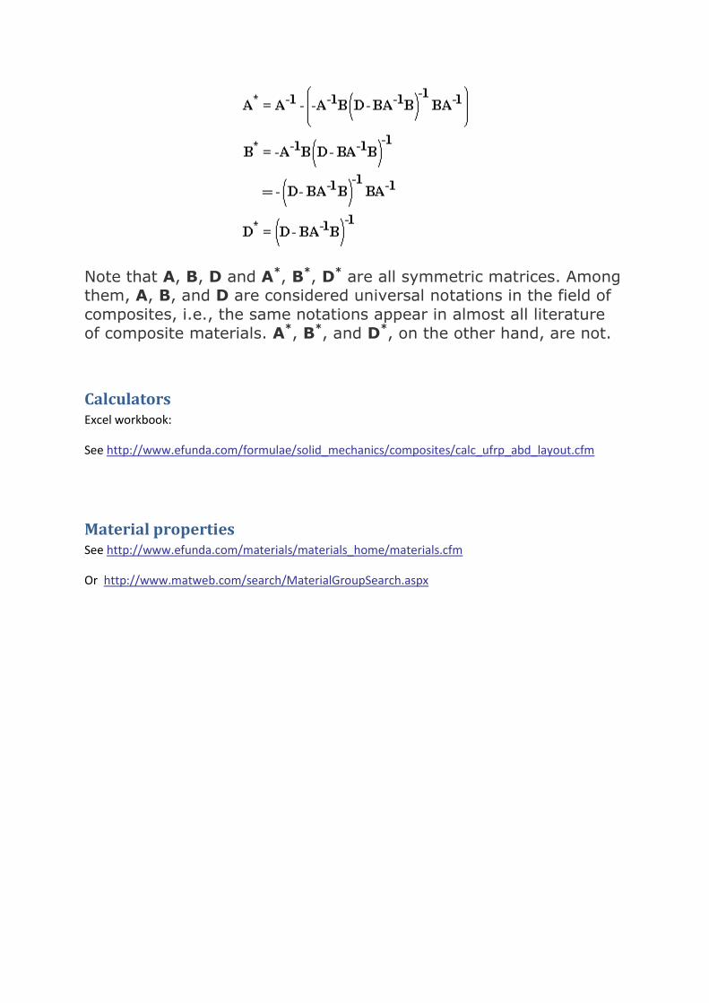
where
Page 22
Note that A, B, D and A*, B*, D* are all symmetric matrices. Among
them, A, B, and D are considered universal notations in the field of
composites, i.e., the same notations appear in almost all literature
of composite materials. A*, B*, and D*, on the other hand, are not.
Calculators Excel workbook:
See http://www.efunda.com/formulae/solid_mechanics/composites/calc_ufrp_abd_layout.cfm
Material properties See http://www.efunda.com/materials/materials_home/materials.cfm
Or http://www.matweb.com/search/MaterialGroupSearch.aspx