Introduction to Computer Vision 3D Vision Lecture 4 Calibration CSc80000 Section 2 Spring 2005 Professor Zhigang Zhu, Rm 4439 http://www-cs.engr.ccny.cuny.edu/~zhu/GC-Spring2005/CSc80000-2-VisionCourse.html
Calibration: Find the intrinsic and extrinsic parameters Problem and assumptions Direct parameter estimation approach Projection matrix approach
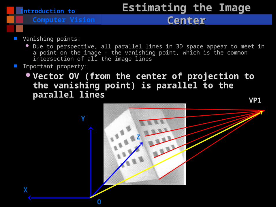
Direct Parameter Estimation Approach Basic equations (from Lecture 5) Estimating the Image center using vanishing points SVD (Singular Value Decomposition) and Homogeneous System Focal length, Aspect ratio, and extrinsic parameters Discussion: Why not do all the parameters together?
Projection Matrix Approach (…after-class reading) Estimating the projection matrix M Computing the camera parameters from M Discussion
Comparison and Summary Any difference?
Introduction to
Computer Vision Problem and AssumptionsProblem and Assumptions Given one or more images of a calibration pattern, Estimate
The intrinsic parameters The extrinsic parameters, or BOTH
Issues: Accuracy of Calibration How to design and measure the calibration pattern
Distribution of the control points to assure stability of solution – not coplanar
Construction tolerance one or two order of magnitude smaller than the desired accuracy of calibration
e.g. 0.01 mm tolerance versus 0.1mm desired accuracy How to extract the image correspondences
Corner detection? Line fitting?
Algorithms for camera calibration given both 3D-2D pairs
Alternative approach: 3D from un-calibrated camera
Introduction to
Computer Vision Camera ModelCamera Model
Coordinate Systems Frame coordinates (xim, yim) pixels Image coordinates (x,y) in mm Camera coordinates (X,Y,Z) World coordinates (Xw,Yw,Zw)
Camera Parameters Intrinsic Parameters (of the camera and the frame grabber): link the
frame coordinates of an image point with its corresponding camera coordinates
Extrinsic parameters: define the location and orientation of the camera coordinate system with respect to the world coordinate system
Zw
Xw
Yw
Y
X
Zx
yO
Pw
P
p
xim
yim
(xim,yim)
Pose / Camera
Object / World
Image frame
Frame Grabber
Introduction to
Computer VisionLinear Version of Perspective ProjectionLinear Version of Perspective Projection
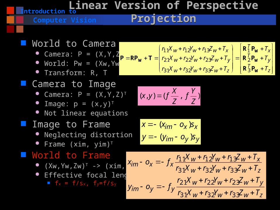
World to Camera Camera: P = (X,Y,Z)T
World: Pw = (Xw,Yw,Zw)T
Transform: R, T
Camera to Image Camera: P = (X,Y,Z)T
Image: p = (x,y)T
Not linear equations
Image to Frame Neglecting distortion Frame (xim, yim)T
World to Frame (Xw,Yw,Zw)T -> (xim, yim)T
Effective focal lengths fx = f/sx, fy=f/sy
zT
yT
xT
zwww
ywww
xwww
T
T
T
TZrYrXr
TZrYrXr
TZrYrXr
w
w
w
w
PR
PR
PR
TRPP
3
2
1
333231
232221
131211
yyim
xxim
soyy
soxx
)(
)(
) ,(),(Z
Yf
Z
Xfyx
zwww
ywwwyyim
zwww
xwwwxxim
TZrYrXr
TZrYrXrfoy
TZrYrXr
TZrYrXrfox
333231
232221
333231
131211
Introduction to
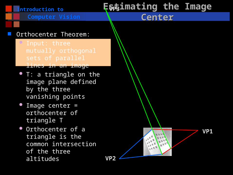
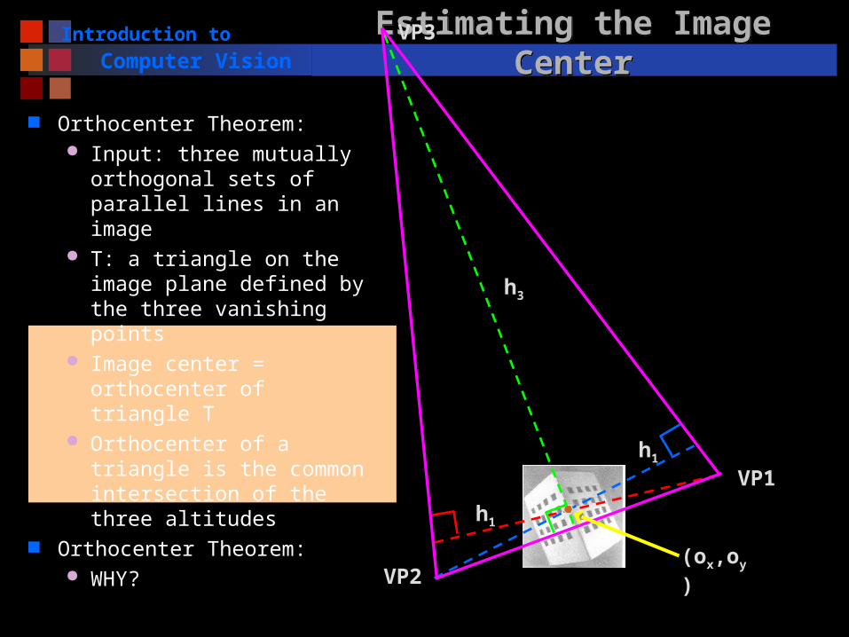
Computer Vision Direct Parameter MethodDirect Parameter Method
Extrinsic Parameters R, 3x3 rotation matrix
Three angles T, 3-D translation vector
Intrinsic Parameters fx, fy :effective focal length in pixel
= fx/fy = sy/sx, and fx (ox, oy): known Image center -> (x,y) known k1, radial distortion coefficient: neglect it in the basic algorithm
Same Denominator in the two Equations Known : (Xw,Yw,Zw) and its (x,y) Unknown: rpq, Tx, Ty, fx, fy
Computer Vision Homogeneous SystemHomogeneous System
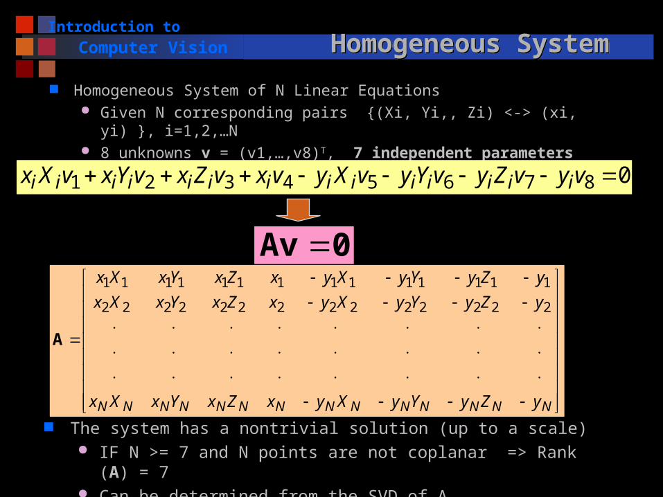
Homogeneous System of N Linear Equations Given N corresponding pairs {(Xi, Yi,, Zi) <-> (xi, yi) }, i=1,2,…N 8 unknowns v = (v1,…,v8)T, 7 independent parameters
087654321 vyvZyvYyvXyvxvZxvYxvXx iiiiiiiiiiiiii
0Av
NNNNNNNNNNNNNN yZyYyXyxZxYxXx
yZyYyXyxZxYxXx
yZyYyXyxZxYxXx
22222222222222
11111111111111
A
The system has a nontrivial solution (up to a scale) IF N >= 7 and N points are not coplanar => Rank (A) = 7 Can be determined from the SVD of A
Introduction to
Computer Vision SVD: definitionSVD: definition
Singular Value Decomposition: Any mxn matrix can be written as the product of three
matricesTUDVA
Singular values i are fully determined by A D is diagonal: dij =0 if ij; dii = i (i=1,2,…,n)
1 2 … N 0
Both U and V are not unique Columns of each are mutual orthogonal vectors
nnnn
n
n
n
mmmm
m
m
mnmm
n
n
vvv
vvv
vvv
uuu
uuu
uuu
aaa
aaa
aaa
21
22212
121112
1
21
22221
11211
21
22221
11211
00
0
0
00
V1U1
Appendix A.6
Introduction to
Computer Vision SVD: propertiesSVD: properties
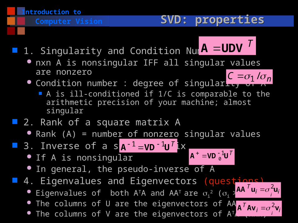
1. Singularity and Condition Number nxn A is nonsingular IFF all singular values are nonzero Condition number : degree of singularity of A
A is ill-conditioned if 1/C is comparable to the arithmetic precision of your machine; almost singular
2. Rank of a square matrix A Rank (A) = number of nonzero singular values
3. Inverse of a square Matrix If A is nonsingular In general, the pseudo-inverse of A
4. Eigenvalues and Eigenvectors (questions) Eigenvalues of both ATA and AAT are i
2 (i > 0) The columns of U are the eigenvectors of AAT (mxm) The columns of V are the eigenvectors of ATA (nxn)
Least Square Solve a system of m equations for n unknowns x(m >= n) A is a mxn matrix of the coefficients b (0) is the m-D vector of the data Solution:
How to solve: compute the pseudo-inverse of ATA by SVD (ATA)+ is more likely to coincide with (ATA)-1 given m > n Always a good idea to look at the condition number of ATA
Homogeneous System m equations for n unknowns x(m >= n-1) Rank (A) = n-1 (by looking at the SVD of A) A non-trivial solution (up to a arbitrary scale) by SVD: Simply proportional to the eigenvector corresponding to the
only zero eigenvalue of ATA (nxn matrix)
Note: All the other eigenvalues are positive because
Rank (A)=n-1 For a proof, see Textbook p. 324-325 In practice, the eigenvector (i.e. vn) corresponding to
Problem Statements Numerical estimate of a matrix A whose entries are not
independent Errors introduced by noise alter the estimate to Â
Enforcing Constraints by SVD Take orthogonal matrix A as an example Find the closest matrix to Â, which satisfies the constraints
exactly SVD of  Observation: D = I (all the singular values are 1) if A is
orthogonal Solution: changing the singular values to those expected
TUDVA ˆ
TUIVA
Introduction to
Computer Vision Homogeneous SystemHomogeneous System
Homogeneous System of N Linear Equations Given N corresponding pairs {(Xi, Yi,, Zi) <-> (xi, yi) }, i=1,2,
…N 8 unknowns v = (v1,…,v8)T, 7 independent parameters
The system has a nontrivial solution (up to a scale) IF N >= 7 and N points are not coplanar => Rank (A) = 7 Can be determined from the SVD of A Rows of VT: eigenvectors {ei} of ATA Solution: the 8th row e8 corresponding to the only zero
singular value 8=0
Practical Consideration The errors in localizing image and world points may make
the rank of A to be maximum (8) In this case select the eigenvector corresponding to the
smallest eigenvalue.
0Av
TUDVA
8ev c
Introduction to
Computer Vision Scale Factor and Aspect RatioScale Factor and Aspect Ratio
Equations for scale factor and aspect ratio
Knowledge: R is an orthogonal matrix
Second row (i=j=2):
First row (i=j=1)
),,,,,,,( 131211232221 xy TrrrTrrr v
T
T
T
ij
rrr
rrr
rrr
r
3
2
1
333231
232221
131211
33R
R
R
R
ji if 0
ji if 1j
Ti RR
1222232221
rrr 23
22
21|| vvv
1222131211
rrr 27
26
25|| vvv
||
v1 v2 v3 v4 v5 v6 v7 v8
Introduction to
Computer Vision Rotation R and Translation TRotation R and Translation T
Equations for first 2 rows of R and T given and ||
First 2 rows of R and T can be found up to a common sign s (+ or -)
The third row of the rotation matrix by vector product
Remaining Questions :
How to find the sign s? Is R orthogonal? How to find Tz and fx, fy?
),,,,,,,( || 131211232221 xy TrrrTrrrs v
yxTT sTsTss ,,, 21 RR
TTTTT ss 21213 RRRRR
T
T
T
ij
rrr
rrr
rrr
r
3
2
1
333231
232221
131211
33R
R
R
R
Introduction to
Computer Vision Find the sign sFind the sign s
Facts: fx > 0 Zc >0 x known Xw,Yw,Zw known
Solution Check the sign of Xc Should be opposite
to xzwww
ywwwyy
zwww
xwwwxx
TZrYrXr
TZrYrXrf
Zc
Ycfy
TZrYrXr
TZrYrXrf
Zc
Xcfx
333231
232221
333231
131211
Zw
Xw
Yw
Y
X
Zx
yO
PwP
p
xim
yim
(xim,yim)
Introduction to
Computer Vision Rotation R : OrthogonalityRotation R : Orthogonality
Question: First 2 rows of R are calculated
without using the mutual orthogonal constraint
Solution: Use SVD of estimate R
TTTTT ss 21213 RRRRR
T
T
T
ij
rrr
rrr
rrr
r
3
2
1
333231
232221
131211
33R
R
R
R
?ˆˆ IRR T
TUDVR ˆ TUIVR
Replace the diagonal matrix D with the 3x3 identity matrix
Introduction to
Computer Vision Find Tz, Fx and FyFind Tz, Fx and Fy
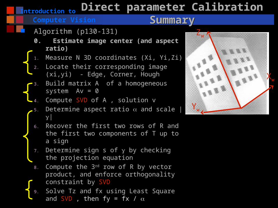
2. Locate their corresponding image (xi,yi) - Edge, Corner, Hough
3. Build matrix A of a homogeneous system Av = 0
4. Compute SVD of A , solution v
5. Determine aspect ratio and scale ||
6. Recover the first two rows of R and the first two components of T up to a sign
7. Determine sign s of by checking the projection equation
8. Compute the 3rd row of R by vector product, and enforce orthogonality constraint by SVD
9. Solve Tz and fx using Least Square and SVD , then fy = fx /
Yw
Xw
Zw
Introduction to
Computer VisionRemaining Issues and Possible SolutionRemaining Issues and Possible Solution
Original assumptions: Without lens distortions Known aspect ratio when estimating image center Known image center when estimating others including aspect ratio
New Assumptions Without lens distortion Aspect ratio is approximately 1, or = fx/fy = 4:3 ; image center about
(M/2, N/2) given a MxN image
Solution (?)1. Using = 1 to find image center (ox, oy)2. Using the estimated center to find others including 3. Refine image center using new ; if change still significant, go to step
2; otherwise stop
Projection Matrix Approach
Introduction to
Computer Vision Linear Matrix Equation of perspective projection
Linear Transform from projective space to projective plane M defined up to a scale factor – 11 independent entries
1w
w
w
ZY
X
w
v
u
extintMM
zT
yT
xT
z
y
x
ext
T
T
T
T
T
T
rrr
rrr
rrr
3
2
1
333231
232221
131211
R
R
R
M
100
0
0
int yy
xx
of
of
M
wv
wu
y
x
im
im
/
/
Introduction to
Computer Vision Projection Matrix MProjection Matrix M
World – Frame Transform Drop “im” and “w” N pairs (xi,yi) <-> (Xi,Yi,Zi) Linear equations of m
3x4 Projection Matrix M Both intrinsic (4) and extrinsic (6) – 10 parameters
1i
i
i
i
i
i
ZY
X
w
v
u
M
34333231
24232221
34333231
14131211
mZmYmXm
mZmYmXm
w
uy
mZmYmXm
mZmYmXm
w
ux
iii
iii
i
ii
iii
iii
i
ii
z
zyyy
zxxx
yyyyyy
xxxxxx
T
ToTf
ToTf
rrr
rorfrorfrorf
rorfrorfrorf
333231
332332223121
331332123111
M
0Am
Introduction to
Computer VisionStep 1: Estimation of projection matrixStep 1: Estimation of projection matrix
World – Frame Transform Drop “im” and “w” N pairs (xi,yi) <-> (Xi,Yi,Zi)
Linear equations of m 2N equations, 11 independent variables N >=6 , SVD => m up to a unknown scale
34333231
24232221
34333231
14131211
mZmYmXm
mZmYmXm
w
uy
mZmYmXm
mZmYmXm
w
ux
iii
iii
i
ii
iii
iii
i
ii
0Am
1111111111
1111111111
10000
00001
yYyYyXyZYX
xZxYxXxZYX
A
Tmmmmmmmmmmmm 343332312423222114131211m
Introduction to
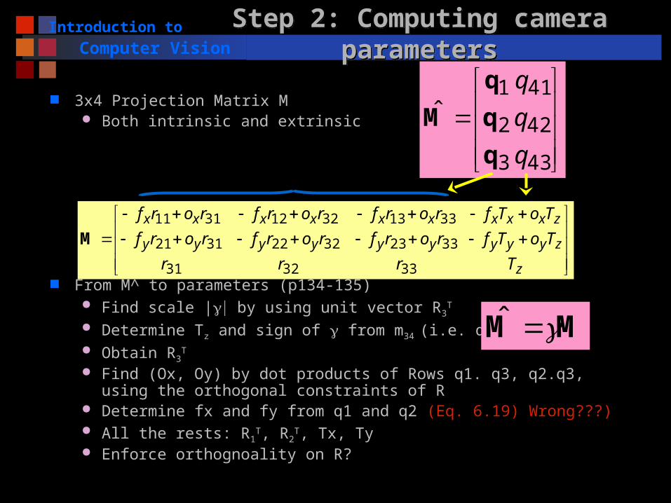
Computer VisionStep 2: Computing camera parametersStep 2: Computing camera parameters
3x4 Projection Matrix M Both intrinsic and extrinsic
From M^ to parameters (p134-135) Find scale | by using unit vector R3
T
Determine Tz and sign of from m34 (i.e. q43) Obtain R3
T
Find (Ox, Oy) by dot products of Rows q1. q3, q2.q3, using the orthogonal constraints of R
Determine fx and fy from q1 and q2 (Eq. 6.19) Wrong???) All the rests: R1
T, R2T, Tx, Ty
Enforce orthognoality on R?
z
zyyy
zxxx
yyyyyy
xxxxxx
T
ToTf
ToTf
rrr
rorfrorfrorf
rorfrorfrorf
333231
332332223121
331332123111
M
MM ˆ
43
42
41
3
2
1ˆ
q
q
q
q
q
q
M
Introduction to
Computer Vision ComparisonsComparisons
Direct parameter method and Projection Matrix method
Properties in Common: Linear system first, Parameter decomposition second Results should be exactly the same
Differences Number of variables in homogeneous systems
Matrix method: All parameters at once, 2N Equations of 12 variables
Direct method in three steps: N Equations of 8 variables, N equations of 2 Variables, Image Center – maybe more stable
Assumptions Matrix method: simpler, and more general; sometime projection
matrix is sufficient so no need for parameter decompostion Direct method: Assume known image center in the first two steps,
and known aspect ratio in estimating image center
Introduction to
Computer Vision Guidelines for CalibrationGuidelines for Calibration
Pick up a well-known technique or a few Design and construct calibration patterns (with known 3D) Make sure what parameters you want to find for your camera Run algorithms on ideal simulated data
You can either use the data of the real calibration pattern or using computer generated data
Define a virtual camera with known intrinsic and extrinsic parameters Generate 2D points from the 3D data using the virtual camera Run algorithms on the 2D-3D data set
Add noises in the simulated data to test the robustness Run algorithms on the real data (images of calibration target) If successful, you are all set Otherwise:
Check how you select the distribution of control points Check the accuracy in 3D and 2D localization Check the robustness of your algorithms again Develop your own algorithms NEW METHODS?