Introduction to Control Systems • Absolute Stability...

MechatronicsControl Systems

K. Craig 1

Control Systems

• Introduction to Control Systems

• Absolute Stability Criteria

• System Performance Specifications

• Modes of Control


K. Craig 2

Introduction to Control Systems

Everything Needs Controlsfor Optimum Functioning!

• Process or Plant• Process Inputs

• Manipulated Inputs• Disturbance Inputs

• Response Variables

Control systems are an integral partof the overall system and not

after-thought add-ons!

Why Controls?• Command Following• Disturbance Rejection

Plant

ManipulatedInputs

DisturbanceInputs

ResponseVariables


K. Craig 3

• Classification of Control System Types– Open-Loop

• Basic

• Input-Compensated Feedforward– Disturbance-Compensated

– Command-Compensated

– Closed-Loop (Feedback)• Classical

– Root-Locus– Frequency Response

• Modern (State-Space)

• Advanced– e.g., Adaptive, Nonlinear, Fuzzy Logic


K. Craig 4

Plant

ControlDirector

ControlEffector

Desired Valueof

Controlled Variable

ControlledVariable

Plant Disturbance Input

PlantManipulated

InputFlow of Energyand/or Material

Basic Open-Loop Control System

Satisfactory if:• disturbances are not too great• changes in the desire value are not too severe• performance specifications are not too stringent


K. Craig 5

Plant

ControlDirector

ControlEffector

Desired Valueof

Controlled Variable

ControlledVariable


PlantManipulated

Input

Flow of Energyand/or Material

DisturbanceSensor

DisturbanceCompensation

Open-Loop Input-Compensated Feedforward Control:Disturbance-Compensated

• Measure the disturbance• Estimate the effect of the disturbance on the

controlled variable and compensate for it


K. Craig 6

Plant

ControlDirector

ControlEffector

Desired Valueof

Controlled Variable

ControlledVariable


PlantManipulated


CommandCompensator

Open-Loop Input-Compensated Feedforward Control:Command-Compensated

Based on the knowledge of plant characteristics, the desired value input is augmented by the command compensator to produce improved performance.


K. Craig 7

• Open-loop systems without disturbance or command compensation are generally the simplest, cheapest, and most reliable control schemes. These should be considered first for any control task.

• If specifications cannot be met, disturbance and/or command compensation should be considered next.

• When conscientious implementation of open-loop techniques by a knowledgeable designer fails to yield a workable solution, the more powerful feedback methods should be considered.


K. Craig 8

Plant

ControlDirector

ControlEffector

Desired Valueof

Controlled Variable

ControlledVariable


PlantManipulated


ControlledVariableSensor

Closed-Loop (Feedback)Control System

Open-Loop Control System is converted to aClosed-Loop Control System by adding:• measurement of the controlled variable• comparison of the measured and desired values of the controlled variable


K. Craig 9

KA

KN

KC

KC

KH

KA

KN

K

Dp

pτ + 1

K

Dp

pτ + 1

Σ

Σ Σ

Σ

C

C

V

V R

R

E

B

M

M

UP

UP

US

+

+

+

+

_

+

+

+

Open-Loop Control System

Closed-Loop Control System

Reference InputElement

Controller Plant

Desired ValueReference

Input

Disturbance

ControlledVariableManipulated

Variable

Sensor(Feedback Element)

SensorError

FeedbackSignal

ActuatingSignal

DisturbanceInput Element


K. Craig 10

Basic Benefits of Feedback Control

• Cause the controlled variable to accurately follow the desired variable.

• Greatly reduce the effect on the controlled variable of all external disturbances in the forward path. It is ineffective inreducing the effect of disturbances in the feedback path (e.g., those associated with the sensor), and disturbances outside the loop (e.g., those associated with the reference input element).

• Are tolerant of variations (due to wear, aging, environmental effects, etc.) in hardware parameters of components in the forward path, but not those in the feedback path (e.g., sensor) or outside the loop (e.g., reference input element).

• Can give a closed-loop response speed much greater than that of the components from which they are constructed.


K. Craig 11

Instability in Feedback Control Systems

• All feedback systems can become unstable if improperly designed.

• In all real-world components there is some kind of lagging behavior between the input and output, characterized by τ’s and ωn’s.

• Instantaneous response is impossible in the real world!

• Instability in a feedback control system results from an improper balance between the strength of the corrective action and the system dynamic lags.


K. Craig 12

Area A

C(t)

+M0 -M0

EDS

Consider the followingexample:• Liquid level C in a tank is manipulated by controlling the volume inflow rate M by means of a 3-position on/off controller.• Transfer function K/Dbetween M and C represents conservation of volume between inflow rate and liquid level.• Liquid-level sensor measures C perfectly but with a data transmission delay, τDT.

Tank Liquid-Level Feedback Control System


K. Craig 13

Clock

TTime

CCControllerDead Zone

+-

SumStep Input

MM

Mo

Flow Rate

K

sPlant

TransportDelay

BB

Tank Liquid-Level Feedback Control System:MatLab / Simulink Block Diagram

3-Position On-Off Controller


K. Craig 14

0 0.5 1 1.5 2 2.5 30

0.5

1

1.5

2

2.5

3

3.5

time (sec)

signal C: solid

signal B: dotted

signal 0.1*M: dashed

Stable Behavior of the Tank Liquid-Level Feedback Control System


K. Craig 15

0 0.5 1 1.5 2 2.5 3-0.5

0

0.5

1

1.5

2

2.5

3

3.5

time (sec)

signal C: solidsignal B: dottedsignal 0.1*M: dashed

Unstable Behavior of the Tank Liquid-Level Feedback Control System


K. Craig 16

Generalized Block Diagram of aFeedback Control System


K. Craig 17

Anti-AliasingFilter

Sensor PlantFinal

ControlElement

A/DConverter

D/AConverter

Digital Computer

SamplingSystem

Sampled & QuantizedMeasurement

Digital Set PointSampled & Quantized

Control Signal

SamplingSwitch

Digital Controlof Dynamic Systems


K. Craig 18

Advantages of Digital Control

• The current trend toward using dedicated, microprocessor-based, and often decentralized (distributed) digital control systems in industrial applications can be rationalized in terms of the major advantages of digital control:– Digital control is less susceptible to noise or parameter

variation in instrumentation because data can be represented, generated, transmitted, and processed as binary words, with bits possessing two identifiable states.


K. Craig 19

– Very high accuracy and speed are possible through digital processing. Hardware implementation is usually faster than software implementation.

– Digital control can handle repetitive tasks extremely well, through programming.

– Complex control laws and signal conditioning methods that might be impractical to implement using analog devices can be programmed.

– High reliability can be achieved by minimizing analog hardware components and through decentralization using dedicated microprocessors for various control tasks.


K. Craig 20

– Large amounts of data can be stored using compact, high-density data storage methods.

– Data can be stored or maintained for very long periods of time without drift and without being affected by adverse environmental conditions.

– Fast data transmission is possible over long distances without introducing dynamic delays, as in analog systems.

– Digital control has easy and fast data retrieval capabilities.

– Digital processing uses low operational voltages (e.g., 0 - 12 V DC).

– Digital control has low overall cost.


K. Craig 21

Discretein

Time

Continuousin

Time

Discretein

Amplitude D-D D-CContinuous

inAmplitude C-D C-C

Digital Signals are:• discrete in time• quantized in amplitude

You must understand the effects of:• sample period

• quantization size


K. Craig 22

• In a real sense, the problems of analysis and design of digital control systems are concerned with taking into account the effects of the sampling period, T, and the quantization size, q.

• If both T and q are extremely small (i.e., sampling frequency 50 or more times the system bandwidth with a 16-bit word size), digital signals are nearly continuous, and continuous methods of analysis and design can be used.

• It is most important to understand the effects of all sample rates, fast and slow, and the effects of quantization for large and small word sizes.


K. Craig 23

sin(6.28t)time

Time

Sum Quantizer4-bit

y_quantized

Quantized

y_continuous

Continuous0.5

Constant

Clock

MatLab / Simulink Block Diagram:Demonstration of Quantization


K. Craig 24

0 0.1 0.2 0.3 0.4 0.5 0.6 0.7 0.8 0.9 10

0.2

0.4

0.6

0.8

1

1.2

1.4

time (sec)

ampl

itud

e: c

onti

nuou

s an

d qu

anti

zed

Simulation of Continuous and Quantized Signal


K. Craig 25

t_discrete

discrete time

discrete_out

discrete out

delayed_out

delayed out

t

continuous time

out

continuous out

Zero-OrderHold

Sample Time: 0.1 sec

Zero-OrderHold

Sample Time: 0.1 sec

TransportDelay: 0.05 sec

Sine Wave

Clock1 Clock

MatLab / Simulink Block Diagram:Demonstration of D/A Conversion

It is worthy to note that the single most important impact of implementing a control system digitally is the delay associated with the D/A converter, i.e., T/2.


K. Craig 26

0 0.1 0.2 0.3 0.4 0.5 0.6 0.7 0.8 0.9 1-1

-0.8

-0.6

-0.4

-0.2

0

0.2

0.4

0.6

0.8

1

time (sec)

ampl

itud

e

Continuous Output and D/A Output


K. Craig 27

Aliasing

• The analog feedback signal coming from the sensor contains useful information related to controllable disturbances (relatively low frequency), but also may often include higher frequency "noise" due to uncontrollable disturbances (too fast for control system correction), measurement noise, and stray electrical pickup.

• Such noise signals cause difficulties in analog systems and low-pass filtering is often needed to allow good control performance.


K. Craig 28

• In digital systems, a phenomenon called aliasingintroduces some new aspects to the area of noise problems.

• If a signal containing high frequencies is sampled too infrequently, the output signal of the sampler contains low-frequency ("aliased") components not present in the signal before sampling. If we base our control actions on these false low-frequency components, they will, of course, result in poor control.

• The theoretical absolute minimum sampling rate to prevent aliasing is 2 samples per cycle; however, in practice, rates of about 10 are more commonly used. A high-frequency signal, inadequately sampled, can produce a reconstructed function of a much lower frequency, which can not be distinguished from that produced by adequate sampling of a low-frequency function.


K. Craig 29

sampled_time

sampled time

sampled

sampled signal

time

analog time

analog

analog signal

Zero-Order Hold: sample time 0.105 sec

Zero-Order Hold:sample time 0.105 sec

Sine Wave10 Hz

Clock

MatLab / Simulink Block Diagram:Demonstration of Aliasing


K. Craig 30

0 0.2 0.4 0.6 0.8 1 1.2 1.4 1.6 1.8 2-0.5

-0.4

-0.3

-0.2

-0.1

0

0.1

0.2

0.3

0.4

0.5

time (sec)

ampl

itud

e: a

nalo

g an

d sa

mpl

ed s

igna

ls

Simulation of Continuous and Sampled Signal


K. Craig 31

Absolute Stability Criteria

• If a system in equilibrium is momentarily excited by command and/or disturbance inputs and those inputs are then removed, the system must return to equilibrium if it is to be called absolutely stable.

• If action persists indefinitely after excitation is removed, the system is judged absolutely unstable.


K. Craig 32

• If a system is stable, how close is it to becoming unstable? Relative stability indicators are gain margin and phase margin.

• If we want to make valid stability predictions, we must include enough dynamics in the system model so that the closed-loop system differential equation is at least third order.– An exception to this rule involves systems with dead

times, where instability can occur when the dynamics (other than the dead time itself) are zero, first, or second order.


K. Craig 33

• The analytical study of stability becomes a study of the stability of the solutions of the closed-loop system’s differential equations.

• A complete and general stability theory is based on the locations in the complex plane of the roots of the closed-loop system characteristic equation, stable systems having all of their roots in the LHP.


K. Craig 34

• Results of practical use to engineers are mainly limited to linear systems with constant coefficients, where an exact and complete stability theory has been known for a long time.

• Exact, general results for linear time-variant and nonlinear systems are nonexistant. Fortunately, the linear time-invariant theory is adequate for many practical systems.

• For nonlinear systems, an approximation technique called the describing function technique has a good record of success.

• Digital simulation is always an option and, while no general results are possible, one can explore enough typical inputs and system parameter values to gain a high degree of confidence in stability for any specific system.


K. Craig 35

• Two general methods of determining the presence of unstable roots without actually finding their numerical values are:– Routh Stability Criterion

• This method works with the closed-loop system characteristic equation in an algebraic fashion.

– Nyquist Stability Criterion• This method is a graphical technique based on the open-loop

frequency response polar plot.

• Both methods give the same results, a statement of the number (but not the specific numerical values) of unstable roots. This information is generally adequate for design purposes.


K. Craig 36

• This theory predicts excursions of infinite magnitude for unstable systems. Since infinite motions, voltages, temperatures, etc., require infinite power supplies, no real-world system can conform to such a mathematical prediction, casting possible doubt on the validity of our linear stability criterion since it predicts an impossible occurrence.

• What actually happens is that oscillations, if they are to occur, start small, under conditions favorable to and accurately predicted by the linear stability theory. They then start to grow, again following the exponential trend predicted by the linear model. Gradually, however, the amplitudes leave the region of accurate linearization, and the linearized model, together with all its mathematical predictions, loses validity.


K. Craig 37

• Since solutions of the now nonlinear equations are usually not possible analytically, we must now rely on experience with real systems and/or nonlinear computer simulations when explaining what really happens as unstable oscillations build up.

• First, practical systems often include over-range alarms and safety shut-offs that automatically shut down operation when certain limits are exceeded. If certain safety features are not provided, the system may destroy itself, again leading to a shut-down condition. If safe or destructive shut-down does not occur, the system usually goes into a limit-cycle oscillation, an ongoing, nonsinusoidal oscillation of fixed amplitude. The wave form, frequency, and amplitude of limit cycles is governed by nonlinear math models that are usually analytically unsolvable.


K. Craig 38

Routh Stability Criterion

• To use the Routh Stability criterion we must have in hand the characteristic equation of the closed-loop system's differential equation.

• Routh's criterion requires the characteristic equation to be a polynomial in the differential operator D. Therefore any dead times must be approximated with polynomial forms in D.


K. Craig 39

• Dead-Time Approximations– The simplest dead-time approximation can be obtained

by taking the first two terms of the Taylor series expansion of the Laplace transfer function of a dead-time element, τdt.

( ) ( )

i

o

i dt dt

q (t) input to dead-time element

q (t) output of dead-time element

q t u t

==

= − τ − τ

( )( )

dt dt

dt dt

u t 1 for t

u t 0 for t <

− τ = ≥ τ

− τ = τDeadTime

qi(t) qo(t)

( ) dtsodt

i

Qs e 1 s

Q−τ= ≈ − τ

( ) ( ) ( )asL f t a u t a e F s− − − = ( ) ( ) io i dt

dqq t q t

dt≈ − τ


K. Craig 40

– The accuracy of this approximation depends on the dead time being sufficiently small relative to the rate of change of the slope of qi(t). If qi(t) were a ramp (constant slope), the approximation would be perfect for any value of τdt. When the slope of qi(t) varies rapidly, only small τdt's will give a good approximation.

– A frequency-response viewpoint gives a more general accuracy criterion; if the amplitude ratio and the phase of the approximation are sufficiently close to the exact frequency response curves of for the range of frequencies present in qi(t), then the approximation is valid.

dtse−τ


K. Craig 41

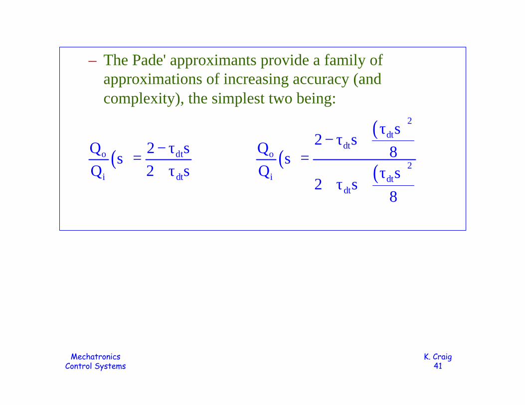
– The Pade' approximants provide a family of approximations of increasing accuracy (and complexity), the simplest two being:

( ) ( )( )

( )

2

dtdt

o dt o2

i dt i dtdt

s2 sQ 2 s Q 8s s

Q 2 s Q s2 s

8

τ− τ +− τ

= =+ τ τ

+ τ +


K. Craig 42

10-1

100

101

102

103

104

105

-400

-350

-300

-250

-200

-150

-100

-50

0

frequency (rad/sec)

phas

e an

gle

(deg

ress

)

Dead-Time Phase-Angle Approximation Comparison

– Dead-time approximation comparison:

( )o dt

i dt

Q 2 ss

Q 2 s

− τ=

+ τ

( )( )

( )

2

dtdt

o2

i dtdt

s2 s

Q 8s Q s

2 s8

τ− τ +

=τ

+ τ +dts

dte 1−τ = ∠−ωτ

τdt = 0.01


K. Craig 43

G1(D)

H(D)

A(D)

N(D)

Σ ΣC

V R E

B

M

U

+

+

_+

G2(D) Z(D)

Q

GeneralizedBlock

Diagram

( ) ( ) ( ) ( ) ( )1 2

H 1A(D)V D Q G D N D U G D Q

Z Z D − + =

[ ] [ ] ( )1 2 1 2 21 G G H(D) Q AG G Z(D) V NZG D U + = +

( )( ) ( ) ( )

( ) ( ) ( )( )

nV nU n1 2 2 1 2

dV dU d

G D G D G DAG G Z(D) NZG D G G H D

G D G D G D≡ ≡ ≡


K. Craig 44

[ ] [ ] ( )

( ) ( )( ) ( ) ( )

1 2 1 2 2

nV nUn

d dV dU

d n nV nU

d dV dU

d nV nU d

d n dV d n dU

d n dV dU d nV dU nU d dV

1 G G H(D) Q AG G Z(D) V NZG D U

G GG1 Q V U

G G G

G G G GQ V U

G G G

G G G GQ V U

G G G G G G

G G G G Q G G G V G G G U

+ = +

+ = +

+= +

= ++ +

+ = +

Closed-Loop System Characteristic Equation:

( )d n dV dUG G G G 0+ =


K. Craig 45

• The terms GdV and GdU are almost always themselves stable (no right-half plane roots) and when they are not stable it is generally obvious since these terms usually are already in factored form where unstable roots are apparent.

• For these reasons it is conventional to concentrate on the term Gn + Gd which came from the original 1 + G1G2H term which describes the behavior of the feedback loop without including outside effects such as A(D), N(D), and Z(D).

• When we proceed in this fashion we are really examining the stability behavior of the closed loop rather then the entire system. Since instabilities in the outside the loop elements are so rare and also usually obvious, this common procedure is reasonable.


K. Craig 46

• We may write the system characteristic equation in a more general form:

• Assume that a0 is nonzero, otherwise the characteristic equation has one or more zero roots which we easily detect and which do not correspond to stable systems.

( )( )( )

( )

1 2

n

d

d n

n n 1n n 1 1 0

1 G G H s 0

G s1 0

G s

G (s) G s 0

a s a s a s a 0−−

+ =

+ =

+ =

+ + + + =L


K. Craig 47

• Routh Criterion Steps– Arrange the coefficients of the characteristic

polynomial into the following array:

– Then form a third row:

– Where

n n 2 n 4 n 6

n 1 n 3 n 5

a a a a

a a a− − −

− − − L

1 2 3b b b L

n 1 n 2 n n 3 n 1 n 4 n n 51 2

n 1 n 1

n 1 n 6 n n 73

n 1

a a a a a a a ab b

a a

a a a ab

a

− − − − − −

− −

− − −

−

− −= =

−= L


K. Craig 48

– When the 3rd row has been completed, a 4th row is formed from the 2nd and 3rd in exactly the same fashion as the 3rd was formed from the 1st and 2nd. This is continued until no more rows and columns can be formed, giving a triangular sort of array.

– If the numbers become cumbersome, their size may be reduced by multiplying any row by any positive number.

– If one of the a's is zero, it is entered as a zero in the array. Although it is necessary to form the entire array, its evaluation depends always on only the 1st column.


K. Craig 49

– Routh's Criterion states that the number of roots not in the LHP is equal to the number of changes of algebraic sign in the 1st column.

– Thus a stable system must exhibit no sign change in first column.

– The Routh criterion does not distinguish between real and complex roots, nor does it give the specific numerical values of the unstable roots.

– Although the complete Routh procedure gives a correct result in every case, two special situations are worth memorizing as shortcuts:

• If the original system characteristic equation itself shows any sign changes, there is really no point in carrying out the Routhprocedure; the system will always be unstable.


K. Craig 50

• If there are any gaps (zero coefficients) in the characteristic equation, the system is always unstable.

• Note, however, that a lack of gaps or sign changes is a necessary but not a sufficient condition for stability.

– Although not of much practical significance, since they rarely occur in practical problems, two special cases can occur mathematically:

a) a term in the first column is zero but the remaining terms in its row are not all zero, causing a division by zero when forming the next row.

b) all terms in the second or any further row are zero, giving the indeterminate from 0/0. This indicates pairs of equal roots with opposite signs located either on the real axis or on the imaginary axis.


K. Craig 51

– The solution for these two special cases is as follows:• For case (a) substitute 1/x for s in the characteristic equation,

then multiply by xn, and form a new array. This method doesn't work when the coefficients of the original characteristic equation and the newly formed characteristic equation are identical. Another solution is to replace the 0 by a very small positive number ε, complete the array and then evaluate the signs in the first column by letting ε → 0. Or another solution is to multiply the original polynomial by (s+1), which introduces an additional negative root, and then form the Routh array.


K. Craig 52

• For case (b) form an auxiliary equation using coefficients from the row above, being careful to alternate powers of s. Differentiate the equation with respect to s to obtain the coefficients of the previously all-zero row. The roots of the auxiliary equation are also roots of the characteristic equation. These roots occur in pairs. They may be imaginary (complex conjungates) or real and equal in magnitude, with one positive and one negative.


K. Craig 53

– Thus for a system to be stable, there must be no sign changes in the first column (to ensure that there are no roots in the RHP) and no rows of zeros (to ensure that there are no pairs of roots on the imaginary axis).

– For example, one sign change in the first column and a row of zeros would imply one real root in the RHP and one real root of the same magnitude in the LHP.

– In addition to answering yes-no questions concerning absolute stability, the Routh criterion is often useful in developing design guidelines helpful in making trade-off choices among system physical parameters.


K. Craig 54

Nyquist Stability Criterion

• The advantages of the Nyquist stability criterion over the Routh criterion are:– It uses the open-loop transfer function, i.e., (B/E)(s), to

determine the number, not the numerical values, of the unstable roots of the closed-loop system characteristic equation. The Routh criterion requires the closed-loop system characteristic equation to determine the same information.


K. Craig 55

– If some components are modeled experimentally using frequency response measurements, these measurements can be used directly in the Nyquist criterion. The Routh criterion would first require the fitting of some analytical transfer function to the experimental data. This involves extra work and reduces accuracy since curve fitting procedures are never accurate.

– Being a frequency response method, the Nyquist criterion handles dead times without approximation since the frequency response of a dead time element, τdt, is exactly known, i.e., the Laplace transfer function of a dead time element is , with an amplitude ratio = 1.0 and a phase angle = - ωτdt.

dtse−τ


K. Craig 56

– In addition to answering the question of absolute stability, Nyquist also gives some useful results on relative stability, i.e., gain margin and phase margin. Furthermore, the graphical plot used, keeps the effects of individual pieces of hardware more apparent (Routh tends to "scramble them up") making needed design changes more obvious.

• While a mathematical proof of the Nyquist stability criterion is available, here we focus on its application and first give a simple explanation of its plausibility.


K. Craig 57

Feedback Control SystemBlock Diagram

Plausibility Demonstration for the Nyquist Stability Criterion


K. Craig 58

– Consider a sinusoidal input to the open-loop configuration. Suppose that at some frequency, (B/E)(iω) = -1 = 1 ∠ 180°. If we would then close the loop, the signal -B would now be exactly the same as the original excitation sine wave E and an external source for E would no longer be required. The closed-loop system would maintain a steady self-excited oscillation of fixed amplitude, i.e., marginal stability.

– It thus appears that if the open-loop curve (B/E)(iω) for any system passes through the -1 point, then the closed-loop system will be marginally stable.

– However, the plausibility argument does not make clear what happens if curve does not go exactly through -1. The complete answer requires a rigorous proof and results in a criterion thatgives exactly the same type of answer as the Routh Criterion, i.e., the number of unstable closed-loop roots. Instead, we state a step-by-step procedure for the Nyquist criterion.


K. Craig 59

1. Make a polar plot of (B/E)(iω) for 0 ≤ ω < ∞ , either analytically or by experimental test for an existing system. Although negative ω's have no physical meaning, the mathematical criterion requires that we plot (B/E)(-iω) on the same graph. Fortunately this is easy since (B/E)(-iω) is just a reflection about the real (horizontal) axis of (B/E)(+iω).


K. Craig 60

Polar Plot of Open-Loop Frequency Response

Simplified Version ofNyquist Stability Criterion

( ) ( )1 2

Bi G G H i

Eω = ω


K. Craig 61

Examplesof

Polar Plots


K. Craig 62

2. If (B/E)(iω) has no terms (iω)k, i.e., integrators, as multiplying factors in its denominator, the plot of (B/E)(iω) for -∞ < ω < ∞ results in a closed curve. If (B/E)(iω) has (iω)k as a multiplying factor in its denominator, the plots for +ω and -ω will go off the paper as ω → 0 and we will not get a single closed curve. The rule for closing such plots says to connect the "tail" of the curve at ω → 0− to the tail at ω → 0+

by drawing k clockwise semicircles of "infinite" radius. Application of this rule will always result in a single closed curve so that one can start at the ω = -∞point and trace completely around the curve toward ω= 0- and ω = 0+ and finally to ω = +∞, which will always be the same point (the origin) at which we started with ω = -∞.


K. Craig 63


K. Craig 64


K. Craig 65


K. Craig 66

3. We must next find the number Np of poles of G1G2H(s) that are in the right half of the complex plane. This will almost always be zero since these poles are the roots of the characteristic equation of the open-loop system and open-loop systems are rarely unstable. If the open-loop poles are not already factored and thus apparent, one can apply the Routh criterion to find out how many unstable ones there are, if any. If G1G2H(iω) is not known analytically but rather by experimental measurements on an existing open-loop system, then it must have zero unstable roots or else we would never have been able to run the necessary experiments because the system would have been unstable. We thus generally have little trouble finding Np and it is usually zero.


K. Craig 67

4. We now return to our plot (B/E)(iω), which has already been reflected and closed in earlier steps. Draw a vector whose tail is bound to the -1 point and whose head lies at the origin, where ω = -∞. Now let the head of this vector trace completely around the closed curve in the direction from w = -∞ to 0- to 0+ to +∞, returning to the starting point. Keep careful track of the total number of net rotations of this test vector about the -1 point, calling this Np-z and making it positive for counter-clockwise rotations and negative for clockwise rotations.


K. Craig 68


K. Craig 69

5. In this final step we subtract Np-z from Np. This number will always be zero or a positive integer and will be equal to the number of unstable roots for the closed-loop system, the same kind of information given by the Routh criterion. The example shows an unstable closed-loop system with two unstable roots since Np = 0 and Np-z = -2.


K. Craig 70

– The Nyquist criterion treats without approximation systems with dead times. Since the frequency response of a dead time element τdt is given by the expression 1∠-ωτdt, the (B/E)(iω) for the system of Figure (a) spirals unendingly into the origin. With low loop gain, the closed-loop system is stable, i.e., Np = 0 and Np-z = 0.

– Raising the gain, Figure (b), expands the spirals sufficiently to cause the test vector to experience two net rotations, i.e., Np-z = -2, causing closed-loop instability. Further gain increases expand more and more of these spirals out to the region beyond the -1 point, causing Np-z to increase, indicating the presence of more and more unstable closed-loop roots.


K. Craig 71

Nyquist Stability Analysis of a System with Dead Time


K. Craig 72

Root-Locus Interpretation of Stability

• The root locus method for analysis and design is a method to find information about closed-loop behavior given the open-loop transfer function.

• The root locus is a plot of the poles of the closed-loop transfer function as any single parameter varies from 0 to ∞.

• The most straightforward method to obtain the root locus is simply to vary the parameter value and use a polynomial root solver to find the poles. However, early techniques in control analysis still give important insights into the design of closed-loop systems.


K. Craig 73

G1(D)

H(D)

A(D)

N(D)

Σ ΣC

V R E

B

M

U

+

+

_+

G2(D) Z(D)

Q

( ) ( ) ( )1 21 KG s G s H s 0+ =Characteristic Equation

of theClosed-Loop System

K is the parameter that is being varied from 0 to ∞.


K. Craig 74

• The root locus begins at the poles of the open-loop transfer function KG1(s)G2(s)H(s) and ends at the zeros of the open-loop transfer function or at infinity.

• Rewrite the closed-loop transfer function as

• This implies that

( ) ( ) ( )1 2KG s G s H s 1= −

( ) ( ) ( )( ) ( ) ( ) ( )

1 2

1 2

KG s G s H s 1

G s G s H s 2k 1 k = 0, 1, 2,

=

∠ = ± + π L


K. Craig 75

• For a point s* in the s plane to be a part of the root locus, the total angle from the poles and zeros of G1(s)G2(s)H(s) to s* must be ± (2k+1)π.

• The gain K that corresponds to this point is found by:

• Consider as an example a system with open-loop transfer function:

( ) ( ) ( )* * *1 2

1K

G s G s H s=

( ) ( ) ( )1 2

B Ks

E s s 1 s 1=

τ + τ +


K. Craig 76

• The closed-loop characteristic equation is given by:

• Assume that τ1 and τ2 have been chosen and we wish to explore the effect of varying loop gain K on system stability. For each value of K, the equation has 3 roots which may be plotted in the complex plane. For K = 0, these roots are 0, -1/τ1, -1/τ2. As K is increased, the roots trace out continuous curves that are called the root loci.

• Every linear, time-invariant feedback system has a root-locus plot and these are extremely helpful in system design and analysis.

( )3 21 2 1 2s s s K 0τ τ + τ + τ + + =


K. Craig 77

( )( )1 2

B K(s)

E s s 1 s 1=

τ + τ +

Root Locus method gives information about closed-loop behavior given the open-loop transfer

function.

The root locus is a plot of the poles of

the closed-loop transfer function as

any single parameter varies

from 0 to ∞.Root-Locus Plot


K. Craig 78

System Performance Specifications

• Basic Considerations• Time-Domain Performance Specifications• Frequency-Domain Performance

Specifications


K. Craig 79

Basic Considerations

• Most of our discussion will involve rather specific mathematical performance criteria whereas the ultimate success of a controlled process generally rests on economic considerations which are difficult to calculate.

• This rather nebulous connection between the technical criteria used for system design and the overall economic performance of the manufacturing unit results in the need for much exercise of judgment and experience in decision making at the higher management levels.


K. Craig 80

• Control system designers must be cognizant of these higher-level considerations but they usually employ rather specific and relatively simple performance criteria when evaluating their designs.


K. Craig 81

• Control System Objective– C follow desired value V and ignore disturbance U

– Technical performance criteria must have to do with how well these two objectives are attained

• Performance depends both on system characteristics and the nature of V and U.

G1(D)

H(D)

A(D)

N(D)

Σ ΣC

V R E

B

M

U

+

+

_+

G2(D) Z(D)

Q

Basic Linear Feedback System


K. Craig 82

• The practical difficulty is that precise mathematical functions for V and U will not generally be known in practice.

• Therefore the random nature of many practical commands and disturbances makes difficult the development of performance criteria based on the actual V and U experienced by real system.

• It is thus much more common to base performance evaluation on system response to simple "standard" inputs such as steps, ramps, and sine waves.


K. Craig 83

• This approach has been successful for several reasons:– In many areas, experience with the actual performance of various

classes of control systems has established a good correlation between the response of systems to standard inputs and the capability of the systems to accomplish their required tasks.

– Design is much concerned with comparison of competitive systems. This comparison can often be made nearly as well in terms of standard inputs as for real inputs.

– Simplicity of form of standard inputs facilitates mathematical analysis and experimental verifications.

– For linear systems with constant coefficients, theory shows that the response to a standard input of frequency content adequate to exercise all significant system dynamics can then be used to find mathematically the response to any form of input.


K. Craig 84

• Standard performance criteria may be classified as falling into two categories: – Time-Domain Specifications: Response to steps,

ramps, and the like

– Frequency-Domain Specifications: Concerned with certain characteristics of the system frequency response

• Both time-domain and frequency-domain design criteria generally are intended to specify one or the other of:– speed of response

– relative stability

– steady-state errors


K. Craig 85

• Both types of specifications are often applied to the same system to ensure that certain behavior characteristics will be obtained.

• All performance specifications are meaningless unless the system is absolutely stable. So we assume absolute stability for the remainder of this discussion.


K. Craig 86

Time-Domain Performance Specifications

• For linear systems, the superposition principle allows us to consider response to commands apart from response to disturbances.

• If both occur simultaneously, the total response is just the superposition of the two individual responses.

• In nonlinear systems, such treatment with subsequent superposition is not valid.


K. Craig 87

• Rise time, Tr, and peak time, Tp, are speed of response criteria.

• Percent overshoot, Op = (O/V) × 100, is a relative stability criterion, with 10% - 20% as an acceptable value.

Closed-Loop Response

of C to a Step of V when U = 0


K. Craig 88

• Settling time, Ts, the time it takes for the response to get and stay within a specified percentage, e.g., 5%, of V, combines stability and speed of response aspects.

• The decay ratio, the ratio of the second overshoot divided by the first, is a relative stability criterion used most often in the process control industry, with 1/4 a common design value.

Which System is Faster?A or B?


K. Craig 89

• Certain math models of systems will predict ,for given commands or disturbances, steady-state errors that are precisely zero, but no really system can achieve this perfection.

• Nonzero errors are always present because of nonlinearities, measurement uncertainties, etc.

• To determine the steady-state error set up the closed-loop system differential equation in which error (V-C) is the unknown. Solution of this equation gives a transient solution that always decays to zero for an absolutely stable system.


K. Craig 90

• The remaining solution is, by definition, the steady-state error, whether it is itself steady or time varying. That is, steady-state error need not be a constant value.

• The steady-state error, Ess, depends on both the system and the input command or disturbance that causes the error.

• There is a certain pattern of behavior as the input is made more difficult from the steady-state viewpoint. This type of pattern can be expected for both commands and disturbances in all linear systems, though details will vary.


K. Craig 91

Effect of Command Severity

on Steady-State Error


K. Craig 92

• For systems in which the feedback element H(s) = 1, i.e., unity-feedback systems, and the reference input element A(s) = 1, the actuating signal E is the system error (V-C), i.e., desired value minus the controlled variable.

• In this case, we can determine the steady-state error Ess by examining the open-loop transfer function G1(s)G2(s).

( ) ( )1 2

1E(s) V(s)

1 G s G s=

+


K. Craig 93

• The final value theorem, assuming closed-loop stability, tells us that:

• We are interested in the steady-state error for step, ramp, and parabolic inputs, i.e.,

• Therefore

sss 0

E limsE(s)→

=

n 1

1V(s) n 0, 1, 2

s += =

ss n ns 01 2

1E lim

s s G (s)G (s)→=

+


K. Craig 94

• System type is the order of the input polynomial that the closed-loop system can track with finite error.

• For example, if G1(s)G2(s) has no poles at the origin, the closed-loop is a Type 0 system and can track a constant with finite steady-state error. A Type 1 system (one pole at the origin) can track a constant with zero error and a ramp with finite error. A Type 2 system (two poles at the origin) can track both a constant and ramp with zero error and a parabola with finite error.


K. Craig 95

• When system input is a disturbance U (V=0) some of these criteria can still be applied, although others cannot.

• It is still possible to define a peak time Tp, however Tr, Ts, and Op are all referenced to step size V, which is now zero, thus they cannot be used.

• One possibility is to use peak value Cp as a reference value to define Tr and Ts.

• To replace Op as a stability specification one could use the decay ratio defined earlier or perhaps the number of cycles to damp the amplitude to say, 10% of Cp. The smaller the number of cycles, the better the stability.

• Definition of steady-state error still applies and we would again expect the same trend of worsening error as U changed from step to ramp to parabola.


K. Craig 96

Time-Domain Performance Specifications

for a Disturbance Input


K. Craig 97

Frequency Response Performance Specifications

• Let V be a sine wave (U = 0) and wait for transients to die out.

• Every signal will be a sine wave of the same frequency. We can then speak of amplitude ratios and phase angles between various pairs of signals.

1 2

1 2

C AG G (i )(i )

V 1 G G H(i )ω

ω =+ ω


K. Craig 98

• The most important pair involves V and C. Ideally (C/V)(iw) = 1.0 for all frequencies.

• Amplitude ratio and phase angle will approximate the ideal values of 1.0 and 0 degrees for some range of low frequencies, but will deviate at higher frequencies.


K. Craig 99

Typical Closed-Loop Frequency Response

Curves


K. Craig 100

• The frequency at which a resonant peak occurs, ωr, is a speed of response criterion. The higher ωr, the faster the system response.

• The peak amplitude ratio, Mp, is a relative stability criterion. The higher the peak, the poorer the relative stability. If no specific requirements are pushing the designer in one direction or the other, Mp = 1.3 is often used as a compromise between speed and stability.

• For systems that exhibit no peak, the bandwidth is used for a speed of response specification. The bandwidth is the frequency at which the amplitude ratio has dropped to 0.707 times its zero-frequency value. It can of course be specified even if there is a peak.


K. Craig 101

• If we set V = 0 and let U be a sine wave, we can measure or calculate (C/U)(iω) which should ideally be 0 for all frequencies. A real system cannot achieve this perfection but will behave typically as shown.

Closed-Loop Frequency Response to a Disturbance Input


K. Craig 102

• Two open-loop performance criteria in common use to specify relative stability are gain margin and phase margin.

• The open-loop frequency response is defined as (B/E)(iω). One could open the loop by removing the summing junction at R, B, E and just input a sine wave at E and measure the response at B. This is valid since (B/E)(iω) = G1G2H(iω). Open-loop experimental testing has the advantage that open-loop systems are rarely absolutely unstable, thus there is little danger of starting up an untried apparatus and having destructive oscillations occur before it can be safely shut down.

• The utility of open-loop frequency-response rests on the Nyquist stability criterion.


K. Craig 103

• Gain margin (GM) and phase margin (PM) are in the nature of safety factors such that (B/E)(iω) stays far enough away from 1 ∠ -180° on the stable side.

• Gain margin is the multiplying factor by which the steady state gain of (B/E)(iω) could be increased (nothing else in (B/E)(iω) being changed) so as to put the system on the edge of instability, i.e., (B/E)(iω)) passes exactly through the -1 point. This is called marginal stability.

• Phase margin is the number of degrees of additional phase lag (nothing else being changed) required to create marginal stability.

• Both a good gain margin and a good phase margin are needed; neither is sufficient by itself.


K. Craig 104

A system must have adequate stability margins.Both a good gain margin and a good phase marginare needed.Useful lower bounds: GM > 2.5 PM > 30°

Open-Loop Performance Criteria:Gain Margin and Phase Margin


K. Craig 105

Bode Plot View ofGain Margin and Phase Margin


K. Craig 106

• It is important to realize that, because of model uncertainties, it is not merely sufficient for a system to be stable, but rather it must have adequate stability margins.

• Stable systems with low stability margins work only on paper; when implemented in real time, they are frequently unstable.

• The way uncertainty has been quantified in classical control is to assume that either gain changes or phase changes occur. Typically, systems are destabilized when either gain exceeds certain limits or if there is too much phase lag (i.e., negative phase associated with unmodeled poles or time delays).

• As we have seen these tolerances of gain or phase uncertainty are the gain margin and phase margin.


K. Craig 107

• Consider the following design problem: Given a plant transfer function G2(s), find a compensator transfer function G1(s) which yields the following:– stable closed-loop system

– good command following

– good disturbance rejection

– insensitivity of command following to modeling errors (performance robustness)

– stability robustness with unmodeled dynamics

– sensor noise rejection


K. Craig 108

• Without closed-loop stability, a discussion of performance is meaningless. It is critically important to realize that the compensator G1(s) is actually designed to stabilize a nominal open-loop plant . Unfortunately, the true plant is different from the nominal plant due to unavoidable modeling errors, denoted by δG2(s). Thus the true plant may be represented by .

• Knowledge of δG2(s) should influence the design of G1(s). We assume here that the actual closed-loop system, represented by the true closed-loop transfer function is absolutely stable.

2G (s)∗

2 2 2G (s) G (s) G (s)∗= + δ

1 2 2

1 2 2

G (s) G (s) G (s)

1 G (s) G (s) G (s)

∗

∗

+ δ + + δ (unity feedback assumed)


K. Craig 109

Design a GoodSingle-Input,

Single-OutputControl Loop

• stable closed-loop system• good command following• good disturbance rejection• insensitivity of command following

to modeling errors• stability robustness with

unmodeled dynamics• sensor noise rejection

Smooth transition from the low to high-frequency

range, i.e., -20 dB/decade slope near the gain

crossover frequency


K. Craig 110

Modes of Control

• On-Off• Proportional• Integral

• Derivative• Combined and Approximate Modes


K. Craig 111

• By mode of control we mean the nature of the behavior of the controller G1(s) in the control system diagram.

G1(D)

H(D)

A(D)

N(D)

Σ ΣC

V R E

B

M

U

+

+

_+

G2(D) Z(D)

Q

Basic Linear Feedback System


K. Craig 112

On-Off Control

• Good design, in general, uses the simplest (and thus usually the least expensive and most reliable) hardware that will meet system performance specifications.

• We should thus try the simplest mode first and go to more complex ones only as the simpler ones are proven inadequate by analysis.

• On-Off controls are generally the simplest possible from a hardware viewpoint. The analysis of on-off control systems, due to nonlinearity, has in the past been difficult or impossible; however, today digital simulation allows us to get essentially exact results for any specific form of system with given numerical values.


K. Craig 113

• For the two-position controller shown, manipulated variable M can take on only two possible values, depending on whether actuating signal E is positive or negative.

• The controller gives the same corrective effort irrespective of whether E is small or large.


K. Craig 114

• Although the nonlinearity of the system prevents application of the Routh or Nyquist stability criteria, it is easily seen that the system is unstable and will go into limit-cycle oscillation (an ongoing, nonsinusoidal oscillation of fixed amplitude).

• M is never off; it is always on in either a positive or a negative sense. Thus controlled variable C is bound to be driven back and forth in a cyclic manner.

• From an energy viewpoint, the controller can supply energy and/or material to the process at only two discrete rates. If neither of these precisely matches the demand of the process, the controller must continually shuttle back and forth between a supply that is too large and one that is too small, giving a limit-cycle instability.


K. Craig 115

• And so we see that on-off controls very often limit cycle and the designer must evaluate the frequency and amplitude of the limit cycle to judge whether such behavior is acceptable.

• For example, most residential heating-cooling systems use on-off control since the limit-cycling behavior is acceptable both in terms of temperature fluctuations being small enough to be comfortable and cycling rates being slow enough to not wear out the switching hardware prematurely.


K. Craig 116

Proportional Control

• Here the manipulating variable M is directly proportional to the actuating signal E.

• We assume that the dynamics associated with the real controller are negligible relative to other system dynamics.

• The corrective effort is made proportional to system "error"; large errors engender a stronger response than do small ones. We can vary in a continuous fashion the energy and/or material sent to the controlled process.

• Relative to on-off control, the advantage is a lack of limit cycling behavior. The disadvantages are general complexity, higher cost, and lower reliability of hardware.


K. Craig 117

• Proportional control exhibits nonzero steady-state errors for even the least-demanding commands and disturbances.

• Why is this so? Suppose for an initial equilibrium operating point xc = xv and steady-state error is zero. Now ask xc to go to a new value xvs. It takes a different value for the manipulated input M to reach equilibrium at the new xc. When the manipulated input M is proportional to the actuating signal E, a new M can only be achieved if E is different from zero which requires xc ≠ xv; thus, there must be a steady-state error.


K. Craig 118

Integral Control

• When a proportional controller can use large loop gain and preserve good relative stability, system performance, including those on steady-state error, may often be met.

• However, if difficult process dynamics such as significant dead times prevent use of large gains, steady-state error performance may be unacceptable.

• When human process operators notice the existence of steady-state errors due to changes in desired value and/or disturbance they can correct for these by changing the desired value ("set point") or the controller output bias until the error disappears. This is called manual reset.


K. Craig 119

• Integral control is a means of removing steady-state errors without the need for manual reset. It is sometimes called automatic reset.

• Integral control can be used by itself or in combination with other control modes. Proportional + Integral (PI) control is the most common mode.

• We have seen why proportional control suffers from steady-state errors. We need a control that can provide any needed steady output (within its design range, of course) when its input (system error) is zero.


K. Craig 120

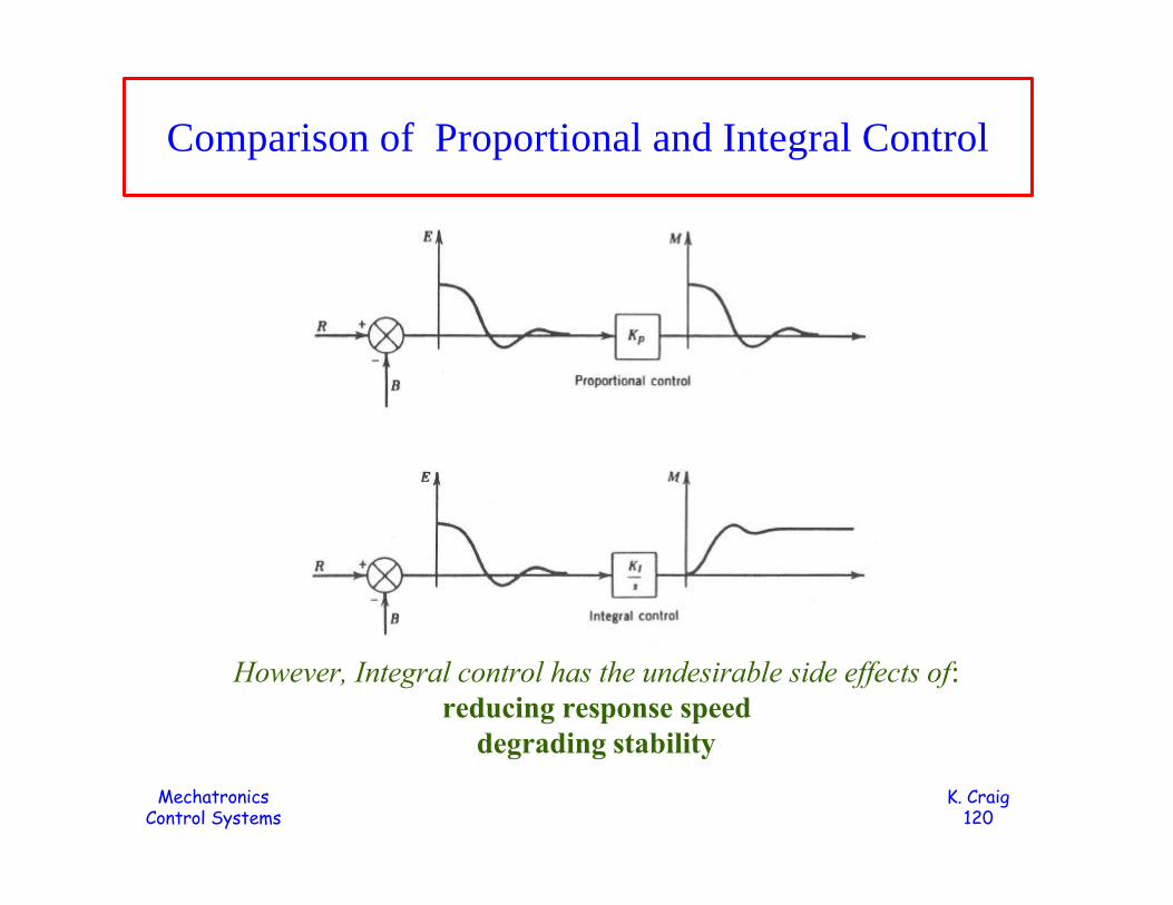
Comparison of Proportional and Integral Control

However, Integral control has the undesirable side effects of:reducing response speed

degrading stability


K. Craig 121

• Although integral control is very useful for removing or reducing steady-state errors, it has the undesirable side effect of reducing response speed and degrading stability.

• Why? Reduction in speed is most readily seen in the time domain, where a step input (a sudden change) to an integrator causes a ramp output, a much more gradual change.

• Stability degradation is most apparent in the frequency domain (Nyquist Criterion) where the integrator reduces the phase margin by giving an additional 90 degrees of phase lag at every frequency, rotating the (B/E)(iω) curve toward the unstable region near the -1 point.


K. Craig 122

• Occasionally an integrating effect will naturally appear in a system element (actuator, process, etc.) other than the controller.

• These gratuitous integrators can be effective in reducing steady-state errors. Although controllers with a single integrator are most common, double (and occasionally triple) integrators are useful for the more difficult steady-state error problems, although they require careful stability augmentation.

• Conventionally, the number of integrators between E and C in the forward path has been called the system type number.


K. Craig 123

From a steady-state error viewpoint, the

"difficulty" of a command or

disturbance is determined by the kind of manipulated-variable

M signal required to return the error to zero

in steady state.


K. Craig 124

• In addition to the number of integrators, their location (relative to disturbance injection points) determines their effectiveness in removing steady-state errors.

• Figure (a) the integrator gives zero steady-state error for a step command but not for a step disturbance.

• By relocating the integrator as in Figure (b), either or both step inputs Vs and Uscan be "canceled" by M without requiring E to be nonzero.


K. Craig 125

• Integrators must be located upstream from disturbance injection points if they are to be effective in removing steady-state errors due to disturbances.

• Location is not significant for steady-state errors caused by commands.


K. Craig 126

Integral (Reset) Windup and its Correction

Integral control may be degraded significantly by saturation effects.


K. Craig 127

• Let's consider the situation of integral windup and its correction. Integral control may be degraded significantly by saturation effects.

• For example, as seen in the figure, a large sustained error causes the integral controller to ramp its output pressure up to the 20-psig supply pressure.

• The diaphragm valve, sized to be wide open at 15 psig (the upper end of the 3 to 15 psig control range) saturates at 15 psig.

• The integral signal beyond t = 7.5 seconds is really useless since it asks for a motion that the valve cannot produce.

• When the error reverses at t = 10 seconds, the valve cannot respond to this change until the integral signal (which has "wound up" to 20 psig) is "unwound" back to the 15-psig level at t = 12.5.

• This delayed response is called reset windup or integral windup.

• Note that this delay is in addition to the normal lagging behavior of integral control and can cause excessive overshooting and stability problems.


K. Craig 128

• Integral windup is of course not a problem in every application of integral control.

• If difficulty is anticipated, the controller can be modified in different ways to give various degrees of improvement.

• Basically, one wants to disable the integrator whenever its output signal causes saturation in the final control element.

• In this example, the integrator is disabled when its output pressure reaches 15 psig, preventing any windup.

• When the error reverses at t = 10 seconds the integrator and valve immediately respond to the negative error since there is no windup that needs to first be unwound.


K. Craig 129

Derivative Control

• On-off, proportional and integral control actions can be used as the sole effect in a practical controller.

• But the various derivative control modes are always used in combination with some more basic control law. This is because the derivative mode produces no corrective effect for any constant error, no matter how large, and therefore would allow uncontrolled steady-state errors.

• One of the most important contributions of derivative control is in system stability augmentation. If absolute or relative stability is the problem, a suitable derivative control mode is often the answer.

• The stabilization or "damping" aspect can easily be understood qualitatively from the following discussion.


K. Craig 130

• Invention of integral control may have been stimulated by the human process operators' desire to automate their task of manual reset. Derivative control hardware may first have been devised as a mimicking of human response to changing error signals. Suppose a human process operator is given a display of system error E and has the task of changing manipulated variable M (say with a control dial) so as to keep E close to zero.


K. Craig 131

• If you were the operator, would you produce the same value of M at t1 as at t2? A proportional controller would do exactly that.

• A stronger corrective effect seems appropriate at t1 and a lesser one at t2 since at t1 the error E is E1,2 and increasing, whereas at t2 it is also E1,2 but decreasing.

• The human eye and brain senses not only the ordinate of the curve but also its trend or slope. Slope is clearly dE/dt, so to mechanize this desirable human response we need a controller sensitive to error derivative.

• Such a control can, however, not be used alone since it does not oppose steady errors of any size, as at t3, thus a combination of proportional + derivative control, for example, makes sense.


K. Craig 132

• The relation of the general concept of derivative control to the specific effect of viscous damping in mechanical systems can be appreciated from the figure below.

• Here an applied torque T tries to control position θ of an inertia J. The damper torque on J behaves exactly like a derivative control mode in that it always opposes velocity dθ/dt with a strength proportional to dθ/dt making motion less oscillatory.


K. Craig 133

• Derivatives of E, C, and almost any available signal in the system are candidates for a useful derivative control mode.

• First derivatives are most common and easiest to implement.

• The noise-accentuating characteristics of derivative operations may often require use of approximate (low-pass filtered) derivative signals.

• Derivative signals can sometimes be realized better with sensors directly responsive to the desired value, rather than trying to differentiate an available signal.

• In addition to stability augmentation, derivative modes may also offer improvements in speed of response and steady-state errors.


K. Craig 134

Combined and Approximate Control Modes

• Proportional + Integral (PI) ControlPhase-Lag Compensation

• Proportional + Derivative (PD) Control

Phase-Lead Compensation• Proportional + Integral + Derivative (PID) Control

Lead / Lag Compensation


K. Craig 135

• We have introduced the basic control modes: on-off, proportional, integral, and derivative. Each of these has its own advantages and drawbacks, and thus it is not surprising that many practical applications are best served by some combination of basic modes.

• We have also considered the most basic or idealized versions of the modes so that their essential features could be brought out most clearly without confusing side issues. Practical versions of some controllers are not able to realize completely the ideal behavior and also may require a modified design technique. Sometimes a non-ideal controller can meet specifications with simpler hardware or software. For these reasons, approximate forms of control modes should be considered.


K. Craig 136

• Phase-Lag Compensation– PI control provides the steady-state-error benefits of

pure integral control with faster response and improved stability.

– Phase-Lag Compensation is the approximate version of PI Control realized in many practical controllers. It cannot attain the zero steady-state errors possible with perfect integral control but this is not a fatal defect because realistic error specifications always must allow some steady-state error.


K. Craig 137

• Phase-Lead Compensation– Since derivative control is never used alone and we

have already briefly discussed PD control, let's concentrate on the approximate version, phase-lead compensation.

– If a basic system has had its gain set for desired relative stability and we then find that its response speed is too slow, phase-lead compensation may be helpful. Also, if a basic system is structurally unstable (gain setting does not provide stability), phase-lead compensation may stabilize the system. Usually, phase-lead compensation also provides a modest gain increase, so steady-state errors are reduced whether this was a problem or not.


K. Craig 138

• Proportional + Integral + Derivative (PID) Control– This combination of basic control modes can improve

all aspects (stability, speed, steady-state errors) of system performance and is the most complex method available as an off-the-shelf general-purpose controller. If we look at analog pneumatic and electronic controllers, their microprocessor-based digital versions, or the individual control loops implemented in a large general-purpose digital process computer, over and over again we see successful applications of P, PI, PD, and PID controls. The basis of the strength of the PID modes is their simplicity; they "make sense."


K. Craig 139

• Lag/Lead Compensation– The approximate version of PID control implemented

in many practical controllers is called lag/lead compensation. Mathematically it is exactly a cascading of the phase-lag and phase-lead controllers already discussed.

– The effects on system performance are also a superposition of the two separate effects, thus a lag/lead controller can improve all aspects of performance (as can a PID): stability, speed, and steady-state errors. Selection of the parameters is performed by essentially designing the two compensators separately.

Date post:	18-Mar-2020
Category:	Documents
Upload:	others
View:	24 times
Download:	2 times

Introduction to Control Systems • Absolute Stability...

Documents