Analysis of Feedback Control Systems Introduction to Feedback Control Systems ................................................................................................... 1
Breaking Apart the Problem to Calculate the Overall Transfer Function ................................... 5
Shortcuts for Calculating Overall Transfer Functions ......................................................................... 5
Inner Feedback Loop Example ................................................................................................................. 6
Feedforward Example .................................................................................................................................. 7
Internal Feedforward Example ................................................................................................................ 8
Developing Block Diagram from Process Equations ............................................................................ 9
Effect of Controller Strategies on First Order Process .......................................................................... 13
Effect of Proportional Control ..................................................................................................................... 14
Effect of PI Control ........................................................................................................................................... 16
Effect of PID Control ........................................................................................................................................ 19
Introduction to Feedback Control Systems
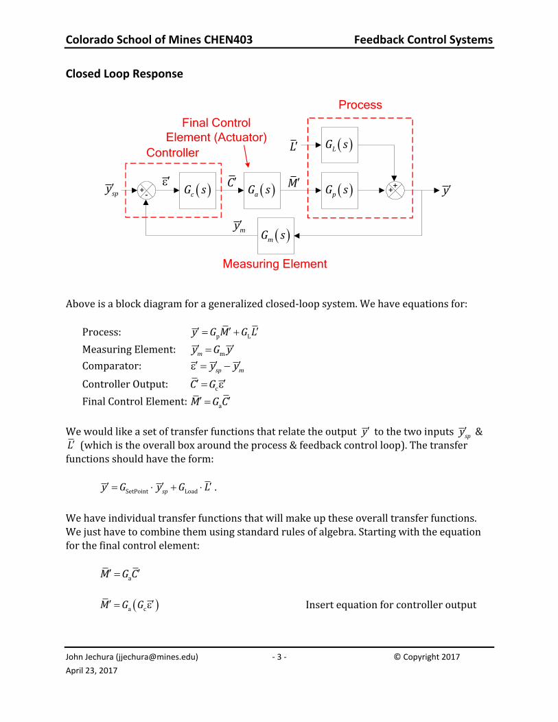
Block diagram of generalized process & corresponding feedback control loop.
+-
y
LG s
cG s ++ pG s
M
L
spy aG s
C
mG smy
Controller
Process
Final Control
Element (Actuator)
Measuring Element
The process has 2 inputs, the disturbance L (also known as the load or the process load) and a measurable variable M , and one output y (the controlled variable). The disturbance
L changes unpredictably. Our goal is to adjust the measurable variable M so that we keep the output variable y as steady as possible. Feedback control takes the following steps:
Colorado School of Mines CHEN403 Feedback Control Systems
• Measure the value of the output, my . • Compare my to the set point, spy . Determine the deviation sp my y . • Deviation processed by controller to give an output signal C to the final control
element. The final control element makes change to the measurable control variable
M . The process itself is referred to as open loop as opposed to when the control is turned on when it is referred to as closed loop. Types of feedback control systems:
• FC — flow control • PC — pressure control • LC — liquid-level control • TC — temperature control • CC — composition control
• Composition: chromatographs, IR analyzers, UV analyzers, pH meters Final control elements are typically valves of some sort. Depending upon situation, specified as fail open or fail close.
Colorado School of Mines CHEN403 Feedback Control Systems
Above is a block diagram for a generalized closed-loop system. We have equations for:
Process: p Ly G M G L
Measuring Element: mmy G y
Comparator: sp my y
Controller Output: cC G
Final Control Element: aM G C
We would like a set of transfer functions that relate the output y to the two inputs
spy & L (which is the overall box around the process & feedback control loop). The transfer
functions should have the form:
SetPoint Loadspy G y G L .
We have individual transfer functions that will make up these overall transfer functions. We just have to combine them using standard rules of algebra. Starting with the equation for the final control element:
aM G C
a cM G G Insert equation for controller output
Colorado School of Mines CHEN403 Feedback Control Systems
Breaking Apart the Problem to Calculate the Overall Transfer Function
+-
y
LG s
cG s ++ pG s
L
spy aG s
mG s Z
This is a lot of math. We can get the same thing by starting with a problem where there are THREE inputs and everything feeds in a forward direction. Consider the block flow diagram above. The relationship between the three inputs is:
p a c L m p a cspy G G G y G L G G G G Z .
However, note that this block diagram is simply the first one we looked at with Z y . So we can make this substitution & do a bit of algebra to get:
p a c L m p a cspy G G G y G L G G G G y
m p a c p a c L1 spG G G G y G G G y G L
p a c L
m p a c m p a c1 1sp
G G G Gy y L
G G G G G G G G
which is what we determined before. Shortcuts for Calculating Overall Transfer Functions
Evaluating the overall transfer function between an input & output can get quite complicated, especially if there are several loads and loops. For a system with a single feedback loop, the transfer function between an input
inY and an output outY is:
Colorado School of Mines CHEN403 Feedback Control Systems
where f is the product of the transfer functions between inY and
outY , is the product of all transfer functions within the loop, and
fn and n are then number of negative signs within the forward path & the loop, respectively. For a simple feedback control loop which only has a negative sign in the comparator the loop law is:
1
fout
in
Y
Y.
If there are multiple loops, then the situation gets more complicated. If the loops are all
embedded and do not cross boundaries then this loop formula can be applied sequentially.
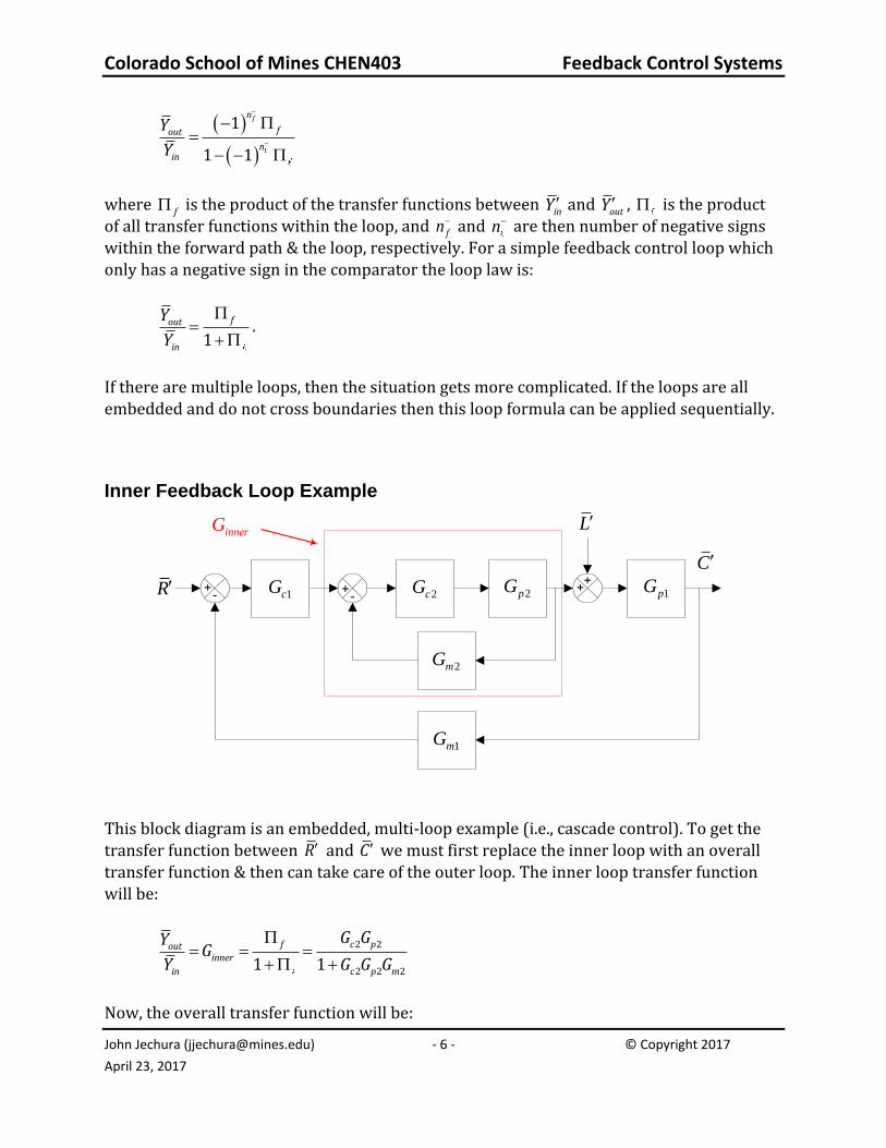
Inner Feedback Loop Example
+-
++R
C
L
1mG
1cG +-
2mG
2cG 2pG 1pG
innerG
This block diagram is an embedded, multi-loop example (i.e., cascade control). To get the transfer function between R and C we must first replace the inner loop with an overall transfer function & then can take care of the outer loop. The inner loop transfer function will be:
2 2
2 2 21 1
f c poutinner
in c p m
G GYG
Y G G G
Now, the overall transfer function will be:
Colorado School of Mines CHEN403 Feedback Control Systems
This block diagram is for a situation where the load information is combined with the output information to give a combined feedforward-feedback control. To get the transfer function between L and C we must consider both forward paths. The output C for the two separate paths involving L will give:
1 1
f v pL
m c v p m c v p
G G GGC L L
G G G G G G G G.
Now, the overall transfer function will be:
1
L f v p
m c v p
G G G GC
L G G G G
Colorado School of Mines CHEN403 Feedback Control Systems
This block diagram is for a situation where the information for the manipulated variable goes through an internal model. (See Chapter 12.) Now there are two feedback loops. We can split off one with the following block diagram. We’ve added a new input (well, kind of, since we really know that Z C ) but we only have one feedback loop.
+-
++R
C
L
mG
cGvG pG
-+
cG
M
Z
The relationship of the output ( C ) to each of the inputs will be:
1 1
c v p m c v p
c v c m c v c m
G G G G G G GC L R Z
G G G G G G G G
(Note that L is not part of the feedback loop!)
1 1c v c m c v c m c v p m c v pG G G G C G G G G L G G G R G G G G Z
Now we take into account that Z C :
Colorado School of Mines CHEN403 Feedback Control Systems
1 1c v c m c v c m c v p m c v pG G G G C G G G G L G G G R G G G G C
1 1m c v p c v c m c v c m c v pG G G G G G G G C G G G G L G G G R
1 1m c v p c c v c m c v pG G G G G C G G G G L G G G R
1
1 1
c v pc v c m
m c v p c m c v p c
G G GG G G GC L R
G G G G G G G G G G
So, the overall transfer functions are:
1
1c v c m
load
m c v p c
G G G GCG
L G G G G G
1
c v p
sp
m c v p c
G G GCG
R G G G G G
.
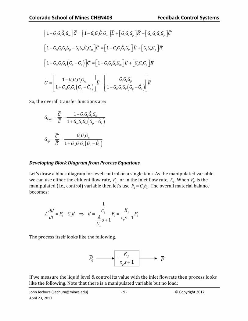
Developing Block Diagram from Process Equations
Let's draw a block diagram for level control on a single tank. As the manipulated variable we can use either the effluent flow rate, 1F , or in the inlet flow rate, 0F . When 0F is the manipulated (i.e., control) variable then let’s use 1 1 1F C h . The overall material balance becomes:
10 1 0 0
1
1
11
p
p
KCdhA F C h h F F
Adt ssC
The process itself looks like the following.
h 1
p
p
K
s
0F
If we measure the liquid level & control its value with the inlet flowrate then process looks
like the following. Note that there is a manipulated variable but no load:
Colorado School of Mines CHEN403 Feedback Control Systems
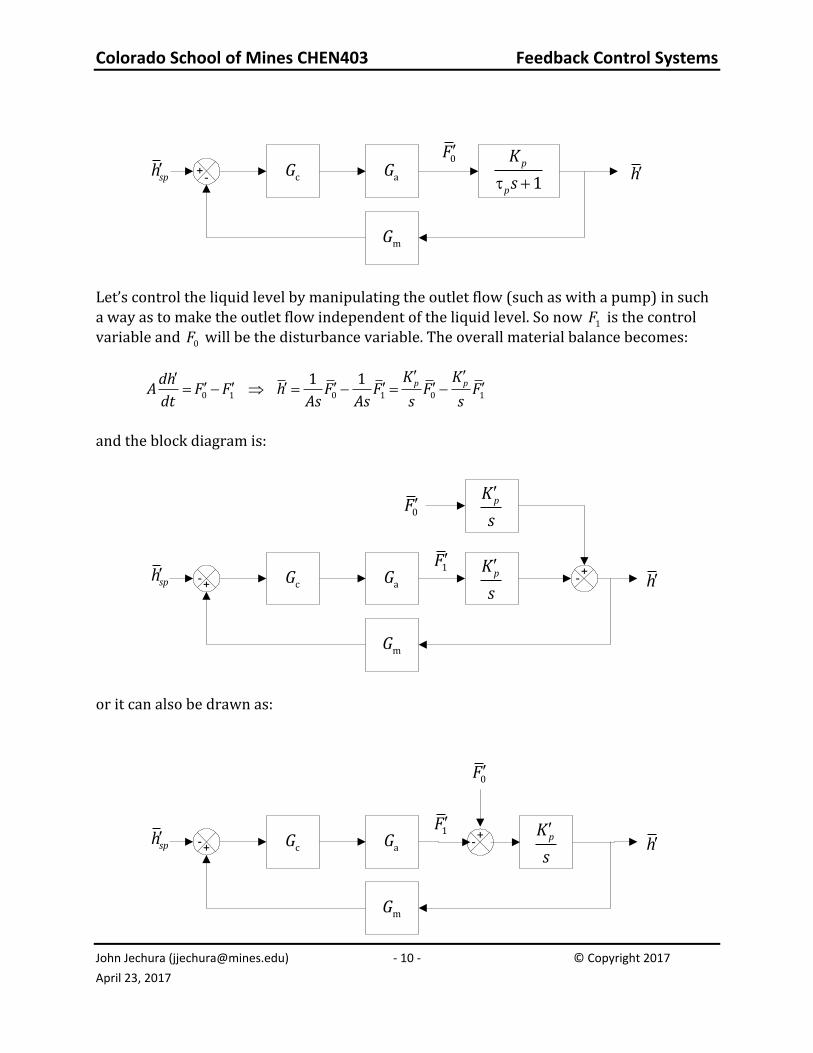
Let’s control the liquid level by manipulating the outlet flow (such as with a pump) in such a way as to make the outlet flow independent of the liquid level. So now 1F is the control variable and 0F will be the disturbance variable. The overall material balance becomes:
0 1 0 1 0 1
1 1 p pK KdhA F F h F F F F
dt As As s s
and the block diagram is:
-+
-+
sph h
0F
mG
cG aG
pK
s
1F
pK
s
or it can also be drawn as:
-+
-+
sph h
0F
mG
cG aG
1F pK
s
Colorado School of Mines CHEN403 Feedback Control Systems
Before we go any further, notice the sign change at the comparator. Normally we define
R mh h , but here we have changed the sign! This is because using 1F to control the liquid level gives what can be thought of as an inverse control type. Normally, if the
measured variable is too small, then the manipulated variable must be increased (e.g., if the temperature in a tank is too low, then the heat to the tank is increased). For the 1st case, control using 0F , if the level is too high, then the flow in must be decreased; if the level is too low, then flow in must be increased. However, here we must go in the opposite direction. If the level is too high, then the flow out must be increased; if the level is too low, then flow out must be decreased. In the block diagram, this logic can be accommodated either by making the control transfer function negative or by changing the signs at the comparator. For the 1st case, using the inlet flow as the manipulated variable, the overall transfer function between the set point and the liquid level will be:
1
1 11
1
p
c v
c v p p c v p
pR c v p m p p c v mc v m
p
KG G
G G G s G G Kh
Kh G G G G s K G G GG G G
s
For the 2nd case, using the outlet flow as the manipulated variable, the overall transfer
function will be:
11
p
c vc v p c v p
pR c v p m p c v mc v m
KG GG G G G G Kh s
Kh G G G G K G G G sG G G
s
Notice that the positions of the negative signs have changed. The other major difference is the form of the process transfer function, pG .
Typical controller strategies
Typical controller strategies and parameter values (SEM pg. 197):
• Proportional (P) control. Controller output will be:
c s cP t K E t P P t K E t
Colorado School of Mines CHEN403 Feedback Control Systems
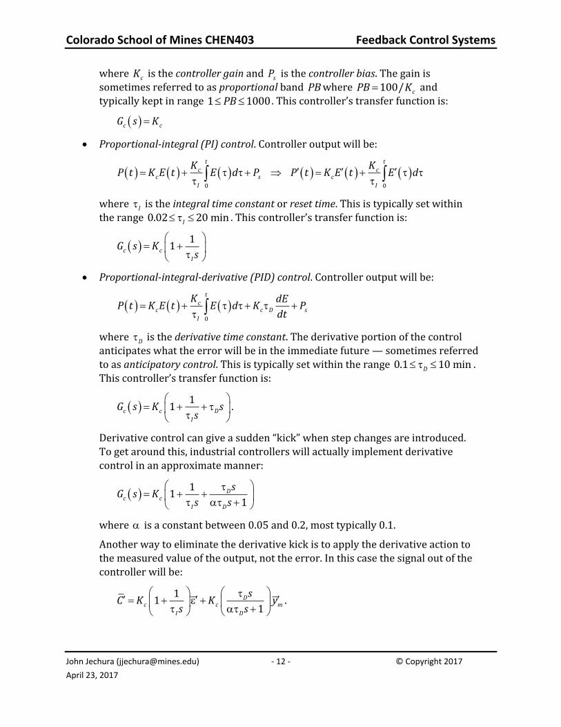
where cK is the controller gain and sP is the controller bias. The gain is sometimes referred to as proportional band PB where 100/ cPB K and typically kept in range 1 1000PB . This controller’s transfer function is:
c cG s K
• Proportional-integral (PI) control. Controller output will be:
0 0
t t
c cc s c
I I
K KP t K E t E d P P t K E t E d
where I is the integral time constant or reset time. This is typically set within the range 0.02 20 minI . This controller’s transfer function is:
11c c
I
G s Ks
• Proportional-integral-derivative (PID) control. Controller output will be:
0
t
cc c D s
I
K dEP t K E t E d K P
dt
where D is the derivative time constant. The derivative portion of the control anticipates what the error will be in the immediate future — sometimes referred to as anticipatory control. This is typically set within the range 0.1 10 minD . This controller’s transfer function is:
11c c D
I
G s K ss
.
Derivative control can give a sudden “kick” when step changes are introduced. To get around this, industrial controllers will actually implement derivative control in an approximate manner:
11
1D
c c
I D
sG s K
s s
where is a constant between 0.05 and 0.2, most typically 0.1.
Another way to eliminate the derivative kick is to apply the derivative action to the measured value of the output, not the error. In this case the signal out of the controller will be:
11
1D
c c m
I D
sC K K y
s s.
Colorado School of Mines CHEN403 Feedback Control Systems
The closed loop block diagram for this type of controller can be expressed like that in the following diagram.
+-
++
spy y
L
mG
c
11
I
Ks
aG pG
LG
C M
my
1D
c
D
sK
s
++
Sometimes, especially with pneumatic transmission lines, there may be a time delay due to signal transmission. This will normally be ignored. However, if the time delay is large enough, then the time delay transfer function will be:
0
1
d s
i p
P s e
P s s.
Effect of Controller Strategies on First Order Process
The controller strategies will have different characteristic effects on a process. A first order process with one manipulated variable and one load will be used to show these effects. Both transfer functions will use the same time constant, p , but different process gains. The underlying ODE and resulting transfer functions will be:
1 1
p Lp p L
p p
p L
K Kdyy K M K L y M L
dt s s
G M G L
Another simplification used here will be to neglect appreciable dynmics from the measuring device & the final control elelment, i.e., 1m aG G .
Colorado School of Mines CHEN403 Feedback Control Systems
The last item is not immediately obvious from the response expression. First, let us define the offset as the difference between a steady state response, y
, and the corresponding set
point:
* *Offset sp sp sp sp spy y y y y y y y
where the expression can be put in terms of deviation variables if the initial steady state is at the initial set point. For a change in the set point and/or the load we can determine the new steady state value by applying the Final Value Thereom.
• For a step change in the set point of sp spy y then the set point’s dynamic function will be:
sp
sp
yy
s
,
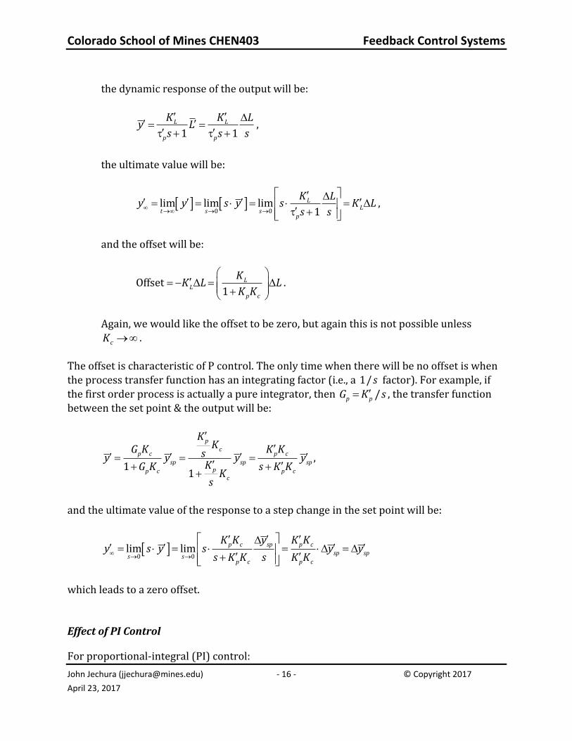
the dynamic response of the output will be:
1 1
p p sp
sp
p p
K K yy y
s s s
,
the ultimate value will be:
0 0
lim lim lim1
p sp
p spt s s
p
K yy y s y s K y
s s
,
and the offset will be:
Offset 1
11
1 1
sp p sp p sp
p c
sp sp
p c p c
y K y K y
K Ky y
K K K K
.
We would like the offset to be zero, but this is not possible unless cK .
• For a step change in the load without a change in set point then 0sp spy y and
L L . The load’s dynamic function will be:
L
Ls
,
Colorado School of Mines CHEN403 Feedback Control Systems
Again, we would like the offset to be zero, but again this is not possible unless
cK . The offset is characteristic of P control. The only time when there will be no offset is when the process transfer function has an integrating factor (i.e., a 1/ s factor). For example, if
the first order process is actually a pure integrator, then /p pG K s , the transfer function between the set point & the output will be:
1
1
p
cp c p c
sp sp sppp c p c
c
KKG K K Ksy y y y
KG K s K KK
s
,
and the ultimate value of the response to a step change in the set point will be:
0 0
lim lim p c sp p c
sp sps s
p c p c
K K y K Ky s y s y y
s K K s K K
which leads to a zero offset. Effect of PI Control
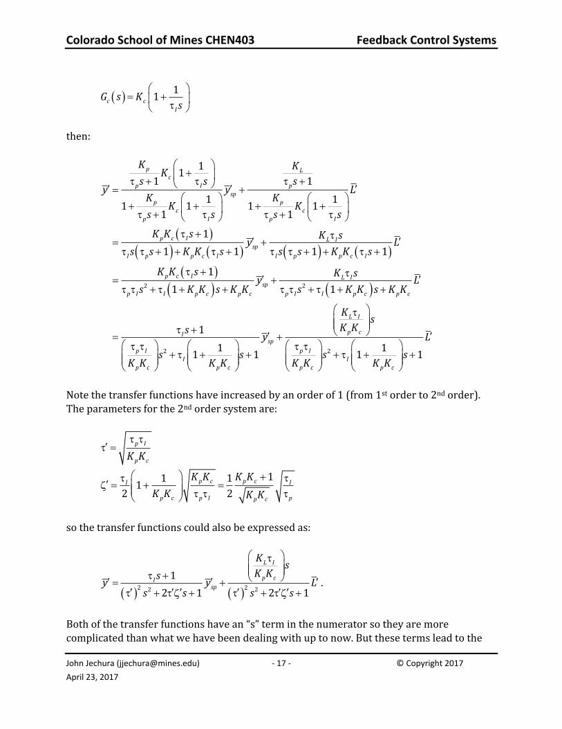
For proportional-integral (PI) control:
Colorado School of Mines CHEN403 Feedback Control Systems
Note the transfer functions have increased by an order of 1 (from 1st order to 2nd order). The parameters for the 2nd order system are:
p I
p cK K
11 1
12 2
p c p cI I
p c p I pp c
K K K K
K K K K
so the transfer functions could also be expressed as:
2 22 2
1
2 1 2 1
L I
p cIsp
Ks
K Ksy y L
s s s s
.
Both of the transfer functions have an “s” term in the numerator so they are more complicated than what we have been dealing with up to now. But these terms lead to the
Colorado School of Mines CHEN403 Feedback Control Systems
property that PI control has zero offset for changes in both the set point and the load. For example, for a step change in the set point of sp spy y then the dynamic response of the output will be:
2 2
1
2 1
spIys
yss s
,
the ultimate value will be:
2 20 0
1lim lim lim
2 1
spIsp
t s s
ysy y s y s y
ss s
,
and the offset will be: Offset 0sp spy y .
The an “s” terms in the numerators will change the expected form of the response curves from “standard” 2nd order system responses.
• For the load, the response will be the derivative of the standard 2nd order response to the driving function. For a ramp change to the load, the response will look like the standard response to a step-change driving function. For a step change in the load,
the response will look like the standard response to an impulse driving function:
2 22 22 1 2 1
L I L I
p c p c
K Ks L
K K K KLy
ss s s s
.
• For the set point, the response have two parts: the standard response with a gain of
one & the derivative of the standard 2nd order response to the driving function. The derivative part will die out after a short period of time leaving the standard response as the long-time solution. For a step change in the set point this will look like a step-change response plus an impulse response:
2 2 22 2 2
1 1
2 1 2 1 2 1
I spsp spIyy ys
ys ss s s s s s
.
Colorado School of Mines CHEN403 Feedback Control Systems
Depending upon the combination of c pK K and /I p the system will be overdamped, underdamped, or critically damped. The following figure shows the relationship of the damping factor to these parameters. Note that for a given I value there is a minimum for an adjustment of cK .
0.0
0.5
1.0
1.5
2.0
2.5
3.0
3.5
4.0
4.5
0 2 4 6 8 10 12
KcKp
'
I/p = 5.0
I/p = 2.5
I/p = 1.0
I/p = 0.5
I/p = 0.25
I/p = 0.1
Effect of PID Control
For proportional-integral-derivative (PID) control:
1
1c c D
I
G s K ss
then:
Colorado School of Mines CHEN403 Feedback Control Systems
Note that the integral action has increased the order of the transfer functions by 1 (from 1st order to 2nd order); the derivative action does not affect this. The parameters for the 2nd order system are:
p I I D p c
p c
K K
K K
/11 11
2 2 1 /
I pp c p cI
p c p I I D p c p c D pp c
K K K K
K K K K K KK K
so the transfer functions could also be expressed as:
2
2 22 2
1
2 1 2 1
L I
p cI D Isp
Ks
K Ks sy y L
s s s s
.
The derivative action will increase the characteristic time but decrease the damping factor . The first action will slow down the response but the second will speed it up. Both affects must be combined to determine the overall affect. Both of the transfer functions have “s” terms in the numerator that lead to zero offsets (primarily from the integral action). The form of the response curve to a load change will
be identical to that for PI control. The response for a set point change, however, has an
Colorado School of Mines CHEN403 Feedback Control Systems
additional short-time contribution that looks like the 2nd derivative of the forcing funciton’s response. For example, for a step change in the set point of sp spy y the dynamic response of the output can be determined from: