arXiv:0907.0668v1 [hep-ph] 3 Jul 2009 INTRODUCTION TO COSMOLOGY A.D. Dolgov ITEP, 117218, Moscow, Russia INFN, Ferrara 40100, Italy University of Ferrara, Ferrara 40100, Italy ITEP Winter School Moscow February 9-14, 2009 Abstract An introductory lectures on cosmology at ITEP Winter School for students specializing in particle physics are presented. Many important subjects are not covered because of lack of time and space but hopefully the lectures may serve as a starting point for further studies. 1 Introduction Modern cosmology is vast interdisciplinary science and it is impossible to cover it in any considerable detail in five hours allocated to me at this School. The task is even more difficult because of different background and level of the participants. Planning these lectures, I have prepared the following short list of subjects, which is surely will be made much shorter at this lecture course, but hopefully it may be useful for the students who would like to continue studying this field. So the idealistic content could be the following: 1. A little about general relativity and its role in cosmology. 2. Four basic cosmological equations and expansion regimes. 3. Universe today and in the past. 4. Kinetics in hot expanding world and freezing of species. 5. Inflation: kinematics, models, universe heating, and generation of density pertur- bations and gravitational waves. 1
Transcript
arX
iv:0
907.
0668
v1 [
hep-
ph]
3 J
ul 2
009
INTRODUCTION TO COSMOLOGY
A.D. Dolgov
ITEP, 117218, Moscow, Russia
INFN, Ferrara 40100, Italy
University of Ferrara, Ferrara 40100, Italy
ITEP Winter School
Moscow
February 9-14, 2009
Abstract
An introductory lectures on cosmology at ITEP Winter School for students
specializing in particle physics are presented. Many important subjects are not
covered because of lack of time and space but hopefully the lectures may serve as a
starting point for further studies.
1 Introduction
Modern cosmology is vast interdisciplinary science and it is impossible to cover it in anyconsiderable detail in five hours allocated to me at this School. The task is even moredifficult because of different background and level of the participants. Planning theselectures, I have prepared the following short list of subjects, which is surely will be mademuch shorter at this lecture course, but hopefully it may be useful for the students whowould like to continue studying this field. So the idealistic content could be the following:
1. A little about general relativity and its role in cosmology.
2. Four basic cosmological equations and expansion regimes.
3. Universe today and in the past.
4. Kinetics in hot expanding world and freezing of species.
5. Inflation: kinematics, models, universe heating, and generation of density pertur-bations and gravitational waves.
7. Field theory at non-zero temperature and cosmological phase transitions.
8. Baryogenesis and cosmological antimatter.
9. Neutrino in cosmology (bounds on mass, oscillations, magnetic moment, and anoma-lous interactions.
10. Dark matter and large scale structure (LSS).
11. Vacuum and dark energies.
12. Cosmic microwave radiation (CMB) and cosmological parameters.
In reality about a half of this plan was fulfilled. At least this lectures could be helpful fora first aquaintance with cosmology and as starting point for deeper studies.
We will start from some non-technical introduction to General Relativity and relationsbetween the latter and cosmology, sec. 2. Next we will derive the basic cosmologicalequations ina rather naive way studying motion of non-relativistic test body in sphericallysymmetric gravitational field, sec. 3. There we also talk about realistic regimes of theuniverse expansion and basic cosmological paramters. In the next section, 4 the universehistory is very briefly presented. Section 5 is dedicated to thermodynamics and kineticsin the early universe. Section 6 is dedicated to freezing of species and cosmological limiton neutrino mass. Big bang nucleosynthesis is presented in sec. 7. In section 8 the role ofneutrinos in BBN is described. Neutrino oscillations in the early universe are consideredin sec. 9. In section 10 inlationary cosmology is discussed, and the last section 11 isdedicated to cosmological baryogenesis.
2 Gravity and cosmology
Two simple observations that the sky is dark at night and that there are shining starslead to the conclusion that the universe is finite in space and time. The first one is thewell known Olbers’ paradox, based on the estimate of the sky luminosity, which in infinitehomogeneous static universe must be infinitely high. Shining stars should exhaust theirfuel in finite time and thus cannot exist in the infinitely old universe – thermal death ofthe universe. General relativity (GR) successfully hit both targets leading to the notionof expanding universe of finite age, but created instead its own very interesting problemswhich we discuss in what follows.
Newtonian theory of gravity has an evident shortcoming that it has action-at-a-distance property. In other words, gravitation acts instantaneously, at any distance. Onthe other hand, in the spirit of contemporary wisdom interactions are always mediatedby some bosonic fields and are relativistically invariant. If we wished today to generaliseNewtonian theory of gravity to relativistic theory we could take, a priori as a mediatorof interactions scalar, vector, or tensor intermediate bosons, confining ourselves to lowerspins.
2
Since we know that gravity operates at astronomically large distances, the mass of theintermediate boson should be zero or very small. Indeed, massless bosons create staticCoulomb type potential, U ∼ 1/r, while massive bosons lead to exponentially cut-offYukawa potential, U ∼ exp(−mr)/r.
Interactions mediated by vector field are odd with respect to charge parity transfor-mation, C-transformation, and as one can see from the vector boson propagator, suchinteractions induce matter-antimatter attraction and matter-matter repulsion, recall elec-tromagnetic interactions. Hence vector field cannot mediate attractive gravitational force.
Scalar and tensor mediators lead to attraction of matter-matter and matter-antimatterand both are a priori allowed. According to non-relativistic Newtonian theory the sourceof gravity is mass. Possible relativistic generalisation for scalars should be a scalar quantitycoinciding in non-relativistic limit with mass. The only known such source is the traceof the energy-momentum tensor of matter, T µ
µ . The relativistic equation of motion forscalar gravity should have the form:
∂2Φ = 8πGNTµµ , (1)
where GN is the Newtonian gravitational coupling constant. Such theory is rejected by theobserved light bending in gravitational field, since for photons: T µ
µ = 0. A small admixtureof scalar gravity to tensor one, i.e. Brans-Dicke theory [1], is allowed.
There remains massless tensor theory with the source which may be only the energy-momentum tensor of matter, Tµν . In first approximation the equation of motion takesthe form:
∂2hµν = 8πGNTµν . (2)
This equation is valid in the weak field approximation because the energy-momentum ofhµν itself should be included to ensure conservation of the total enegy-momentum.
Massless particles, as e.g. gravitons, must interact with a conserved source. Oth-erwise theory becomes infrared pathological. The energy-momentum tensor of matteris conserved only if the energy transfer to gravitational field is neglected. Taking intoaccount energy leak into gravity leads to non-linear equations of motion and allows toreconstruct GR order by order. For a discussion of this approach see papers [2].
Historically Einstein did not start from field theoretical approach but formulated gen-eral relativity in an elegant and economical way as geometrical theory postulating thatmatter makes space-time curved and that the motion of matter in gravitational field issimply free fall along geodesics of this curved manifold. This construction is heavily basedon the universality of gravitational action on all types of matter – the famous equivalenceprinciple, probably first formulated by Galileo Galilei. The least action principle for GRwas formulated by Hilbert with the action given by
A =1
16πGN
∫
d4x√−gR+ Am, (3)
where R is the curvature scalar of four dimensional space-time and and Am is the matteraction, written in arbitrary curved coordinates. Gravitational field is identified with the
3
metric tensor, gµν , of the curved space-time. The curvature is created by matter throughequations of motion:
Rµν −1
2gµνR = 8πGNTµν , (4)
where Rµν is the Ricci tensor. There is no space here to stop on technicalities of Riemanngeometry. A good introduction can be found e.g. in book [3] where one can find definitionand properties of the Christoffel symbols, Γα
The source of gravity is the energy-momentum tensor of matter taken in this curvedspace-time:
Tµν = 2δAm/δgµν . (5)
The impact of gravity on matter is included into Tµν due to its dependence on metric andin some more complicated cases on the curvature tensors. Let us repeat that the motionof matter in the gravitational field is simply the free fall, i.e. motion along geodesics.
Classical tensor theory of gravity agrees with all available data and is a self-consistent,very beautiful and economic theory. It is essentially based on one principle of general co-variance, which is a generalisation of Galilei principle of relativity to arbitrary coordinateframes. Invariance with respect to general coordinate transformation (which is called gen-eral covariance) is a natural framework which ensures vanishing of the graviton mass, mg.Even if the underlying classical theory is postulated to be massless, quantum correctionsshould generally induce non-zero mass if they are not prevented from that by some sym-metry principle. This is another advantage of tensor gravity with respect to scalar one forwhich no principle which forbids non-zero mass is known. Though quantum gravity is notyet understood, it is natural to expect that quantum corrections should induce mg 6= 0 inabsence of general covariance.
An important property of equations of motion (4) is that their right hand side iscovariantly conserved:
Dµ
(
Rµν −1
2gµνR
)
≡ 0. (6)
Accordingly the energy-momentum tensor must be conserved too:
DµTµ (m)ν = 0. (7)
Here, Dµ is covariant derivative, as we have already mentioned. To those not familiarwith Riemann geometry it may be instructive to mention that covariant derivative appearswhen one differentiates in curved coordinate system, e.g. in spherical one, even in flatspace-time. From another point of view, covariant derivative in curved space-time, which,e.g. is acting on vector field, looks as
DµVν = ∂µVν − ΓαµνVα. (8)
4
It is similar to covariant derivative in gauge theories, because the latter includes gaugefield, Aµ analogous to Γα
µν .According to the Noether theorem, the conservation of Tµν follows from the least
action principle if the matter action is invariant with respect to general coordinate trans-formation. So the gravitational (Hilbert) part of the action and the matter part lead toself-consistent equations of motion only if general covariance is maintained.
There is a deep analogy between the Einstein gravity and Maxwell electrodynamics.The Maxwell equations have the form:
∂µFµν = 4πJν (9)
Owing to anti-symmetry of F µν , the l.h.s. is automatically conserved:
∂µ∂νFµν ≡ 0, (10)
so the current must be conserved too:
∂µJµ = 0. (11)
These two conditions are consistent due to gauge invariance of the total electromagneticaction with matter included.
Einstein was the first who decided to apply GR equations (4) to cosmology in 1918and was very much disappointed to find that the equations do not have static solutions.So an advantage of GR was erroneously taken as a shortcoming. Only after the Friedmansolution in 1922 which predicted the cosmological expansion [4] and the Hubble discoveryof the latter in 1929 [5], the idea that our world is not stationary and may have a finitelife-time was established.
The distribution of matter in the universe is assumed to be homogeneous and isotropic,at least in the early stage, as indicated by isotropy of cosmic microwave backgroundradiation (CMB), and even now at large scales. Correspondingly the metric can be takenas homogeneous and isotropic one (FRW metric [6]):
ds2 = dt2 − a2(t)[
f(r)dr2 + r2dΩ]
, (12)
where the function f(r) describes 3D space of constant curvature, f(r) = 1/(1 − kr2).The evolution of the scale factor a(t), i.e. the expansion law, is determined by the
Friedman equations, which follow from the general GR ones for the FRW anzats. Thederivation is straightforward but quite tedious. We will derive them in the next sectionin very simple but not rigourous way. The derivation may be taken as a mnemonic ruleto recall the equations in one-two minutes.
3 Cosmological expansion
3.1 Basic cosmological equations
Here we will present an oversimplified derivation of the Friedman equations. Thoughthe arguments are subject to criticism, the final results are correct. Let us consider a
5
test body on the surface of homogeneous sphere with radius a(t) and the energy den-sity ρ. The energy conservation condition for the non-relativistic test particle readsv2/2 = GNM/a + const where M = 4πa3ρ/3. It can be rewritten as:
H2 ≡(
a
a
)2
=8π ρGN
3− k
a2(13)
This is one of the main cosmological equations. Here is the famous Hubble expansion law,that the object situated at distance d runs away from us with velocity proportional tothe distance, v = Hd. Notice that for d > 1/H it runs away with superluminous velocity.Superluminous velocities of distant objects are allowed by GR but locally velocities mustbe always smaller or equal to the speed of light.
Another equation follows from the energy balance of the medium inside the sphere:dE = −P dV where E = ρV and dE = V dρ+ 3(da/a)V ρ. Hence:
ρ+ 3H(ρ+ P ) = 0. (14)
This equation is simply the law of covariant energy-momentum conservation (7) in metric(12).
Problem 1. Derive from eqs. (13) and (14) the law for the acceleration of the testbody:
a
a= −4π GN
3(ρ+ 3P ) (15)
A striking feature of equation (15) is that not only energy but also pressure gravitates.It is always assumed in canonical theory that ρ is positive, though pressure may benegative. Thus if ρ+3P < 0, the cosmological expansion would proceed with acceleration,i.e. antigravity may operate in cosmological scales. In other words, negative pressure isthe source of the cosmological expansion. Life is possible only because of that. We believethat the universe was in such anti-gravitating state at the very beginning, during the socalled inflationary stage (see below). Surprisingly it was established during the last decadethat at the present time the expansion is also accelerating. There existed a simple analogybetween the universe expansion and the motion of a stone thrown up from the Earth withsome initial velocity v0. The speed of the stone drops down with time and it either willreturn back to the Earth, if v0 is smaller than a certain value, v1. If v0 > v1 the stonewill never come back. In the last case the stone will either come to infinity with non-zerospeed or with the vanishing one. All three such regimes could exist in cosmology andthey were believed to be realised, depending upon the initial expansion velocity. Thefirst regime corresponds to the closed universe with ρ > ρc, where ρc is the critical orclosure energy density, see below. The expansion in this case will ultimately turn intocontraction. The other two regimes correspond to open universe which was expected toexpand forever. The third one with zero velocity at infinity corresponds to spatially flatuniverse, with k = 0 in eq. (13). Now the picture is very much different. Imagine thatyou have thrown a stone from the Earth and first the stone moves with normal negativeacceleration and after a while starts to move faster and faster as if it has a rocket engine.This is exactly what we see in the sky now. It means, in particular, that the spatially
6
closed universe may expand forever. This accelerated cosmological expansion, induced byantigravity at cosmological scale is prescribed to existence of mysterious dark energy. Itis one the greatest unsolved problems in modern fundamental physics.
Problem 2. We seemingly started from the Newtonian theory but came to the con-clusion that pressure gravitates which is not the true in Newtonian case. Where is thedeviation from Newton?Problem 3. Prove that for positive definite energy density, ρ > 0, any object of finite sizecreates an attractive gravitational force, even if inside such an object pressure may bearbitrary negative.Problem 4. Prove that any finite object with positive energy density gravitates, so anti-gravitational action of pressure can manifest itself only in infinitely large objects.
Except for equations which determine the law of the cosmological expansion, we needan equation which governs particle propagation in FRW metric, i.e. geodesic equation.The latter can be written as:
dV α
ds= −Γα
µνVµV ν + curvature term, (16)
where V α = dxα/ds and the curvature term is absent in spatially flat universe, whenk = 0. In what follows we will consider only this case, moreover, the effects of curvatureare typically small.
To solve this equation one needs first to calculate the Christoffel symbols for metric(12). In 3D flat space they have very simple form:
Γijt = Hδi
j, Γtij = Ha2δij. (17)
All other are zero. After that the geodesic equation takes a very simple form:
p = −Hp (18)
with an evident solution p ∼ 1/a(t) which describes red-shifting of momentum of a freeparticle moving in FRW background. In derivation of this result one has to pay attentionthat physical momentum is defined with respect to physical length dl = a(t)dx.
We can simply derived the same result taking into account the Doppler red-shift ofthe momentum of a free particle induced by the cosmological expansion. Let us take twopoints A and B separated by distance dl. The relative velocity of these two points due toexpansion is U = Hdl. The Doppler shift of the momentum of the particle moving fromA to B with velocity v = dl/dt is
dp = −UE = −HEdl. (19)
Thus
p = −HEdl/dt = −Hp. (20)
Let introduce at this stage the notion of the cosmological red-shift:
z = a(tU)/a(t) − 1, (21)
7
where tu is the universe age and a(tU) is the value of the scale factor today. So the mo-mentum of a free particles drops down in the course of expansion as p ∼ 1/a ∼ 1/(z + 1).
Equations (13-15) are the basic cosmological equations for three unknowns, a, ρ, andP . However, there are only two independent equations. So it is necessary to have onemore equation describing properties of matter i.e. the equation of state (e.o.s.): P = P (ρ).Usually this equation is parametrized in the simple linear form:
P = wρ. (22)
The parameter w determines matter properties. For non-relativistic matter pressure isnegligibly small in comparison with ρ and in a good approximation we can take w = 0.For relativistic matter w = 1/3. There is also one more type of matter (or vacuum) knownto exist in the universe, for which w = −1.
However, sometimes the equation of state does not exist but the necessary additionalrelation (not e.o.s.) can be derived from the equations of motion. E.g. for a scalar field:
D2φ+ U ′(φ) = 0 (23)
and one can calculate Tµν and find ρ and P but P 6= P (ρ).Problem 5. Calculate Tµν(φ), ρ, and P for homogeneous field φ(t).
3.2 Expansion regimes
Here we will present solutions of the cosmological equations for several special cases whichwere/are realised in the universe at different stages of her evolution. We always assumethat the three dimensional space is flat, i.e. k = 0. As we see below it is true duringpractically all life-time of the universe.
Let us first consider non-relativistic matter with equation of state P = 0. Accordingto eq. (14) the evolution of the energy density is given by:
ρ = −3Hρ (24)
and thus ρ ∼ 1/a3. The result is evident, it is simply dilution of the number density ofmassive particle at rest.
The time dependence of the cosmological scale factor, is determined by eq. (13):
a/a ∼ √ρ (25)
and thus in non-relativistic regime a ∼ t2/3 and H = 2/3t.For relativistic matter the equation of state is P = ρ/3 and correspondingly
ρ = −4Hρ. (26)
Thus ρ drops as ρ ∼ 1/a4 and the scale factor rises as a(t) ∼ t1/2, which means thatH = 1/2t.
The energy density of relativistic particles drops one power of a faster than that ofnon-relativistic ones due to dilution of their number density as volume, 1/a3, and red-shift
8
of the particle momentum. That’s why relativistic matter dominated in the early universe,while at a later stage non-relativistic matter took over. Until last years of the XX centuryit was believed that the universe today is dominated by non-relativistic matter but thenit was established that the dominant matter is the so called dark energy with equation ofstate close to the vacuum one.
In the vacuum(-like) regime the energy-momentum tensor is proportional to the metrictensor which is the only invariant tensor:
Tµν = ρvac gµν . (27)
Hence Pvac = −ρvac and vacuum energy density remains constant in the course of thecosmological expansion: ρ = −3H(ρ+ P ) = 0. The scale factor in this case rises expo-nentially a ∼ exp(Ht).
According to our understanding, all visible universe originated from microscopicallysmall volume with negligible amount of matter by exponential expansion with practicallyconstant ρ, see below.
It is interesting to calculate the causality distance as a function of time, which is equalto the light path propagating from an initial moment t1 = 0 to final moment t2. Thisdistance can be found from the light geodesic equation: dt2 − a2(t)dr2 = 0. It can beeasily integrated to give:
lγ = a(t)
∫ t
0
dt′
a(t′). (28)
Thus for relativistic regime, lγ = 2t, for non-relativistic one it is lγ = 3t, and for expo-nential De Sitter (inflationary stage): lγ = H−1[exp(Ht) − 1].
As we see, cosmological equations do not have stationary solutions, at least for theexamples taken. In the case of positive space curvature, i.e. k > 0, and normal matterwith ρ ∼ 1/an, n=3,4, the expansion will ultimately change into contraction. If however,ρ > k/a2, e.g. if ρ is vacuum energy, the expansion may last forever for any k.
Note, that if the cosmological energy density is dominated by the normal matter theHubble parameter drops down as H ∼ 1/t, where t is the universe age. If the universe isdominated by vacuum(-like) energy, the Hubble parameter remains constant,
Problem 6. Find ρ(a) and a(t) for general linear equation of state, P = wρ witharbitrary w. Study the case of w ≤ −1.
3.3 Cosmological parameters
Before proceeding further let us say a few words about the natural system of units whichis used throughout all these lectures. We take speed of light, reduced Planck constant,and Boltzmann constant all equal to unity. c = h/2π = k = 1. All dimensional quantitieshave dimension of length, or time, or (inverse) mass or energy – all the same. For ex-ample the Newtonian gravitational constant has dimension of inverse mass, GN ≡ 1/M2
P l;MP l = 1.221 · 1019 GeV = 2.176 · 10−5 g; mp = 938 MeV = 1.67 · 10−24 g;1 GeV−1 = 1.97 · 10−14 cm = 0.66 · 10−24, s; 1 eV = 1.16 · 104Ko.
9
Homogeneous cosmology is described in terms of the Hubble parameter H = a/a,which characterises the universe expansion rate, by the critical or closure energy density
ρc = 3H2M2P l/8π (29)
and by the dimensionless parameter Ωj = ρj/ρc, which measures the relative contributionof the energy density of species of type j into the total energy density of the universe.Clearly for spatially flat universe the total energy density is equal to the critical one:Ωtot = 1, if k = 0. It remains constant in the course of the universe expansion.
If k 6= 0, then from eq. (13) follows that Ω evolves with time as
Ω(a) =
[
1 −(
1 − 1
Ω0
)
ρ0a20
ρa2
]−1
, (30)
where the index sub-0 denotes the present day values of the corresponding quantities.For normal matter ρa2 → 0 if a→ ∞ and Ω runs away from unity: Ω(a) → 0 if Ω0 < 1
and Ω(a) → ∞ if Ω0 > 1. On the other hand, Ω(a) → 1 when ρa2 → ∞, e.g. for vacuumenergy at expansion for arbitrary initial Ω.
The present day value of the H characterises by dimensionless parameter h as
H = 100 h km/sec/Mps, (31)
where h = 0.73 ± 0.05. The inverse quantity H−1 = 9.8 Gyr/h ≈ 13.4 Gyr is approxi-mately equal to the universe age.
An exact expression for the universe age through the present day values of the Hubbleparameter and relative energy densities of different forms of matter can be obtained byintegration of the equation
a =[
8π ρGN a2/3 − k
]1/2(32)
After simple algebra one finds:
tU =1
H
∫ 1
0
dx√
1 − Ωt + Ωm
x+ Ωr
x2 + x2Ωv
, (33)
where Ωt is the total Ω and Ωr,m,v are respectively contributions from relativistic andnon-relativistic matter and from vacuum energy. All the quantities in this equations arethe present day ones; we skipped the sub-index 0 here.
Problem 7. Derive eq. (33). Find tU for Ωt = Ωm = 0, 0.3, 1. Find tU for Ωt = 1,Ωm = 0.3, and Ωv = 0.7.
The “measured” value of the universe age lies in the interval
tU = 12 − 15 Gyr, (34)
found from the ages of old stellar clusters and nuclear chronology.The present day value of the critical energy density is :
ρc =3H2m2
P l
8π= 1.88 · 10−29h2 g
cm3= 10.5 h2keV
cm3≈ 10−47h2 GeV4 (35)
It corresponds approximately to 10 protons per m3, but the dominant matter is not thebaryonic one and in reality there are about 0.5 protons per cubic meter.
10
3.4 Matter inventory
The relative contributions of different forms of matter into the total energy density areobtained from different independent astronomical observations. Here we only presenttheir numerical values. For discussion of their measurements in more detail a few extralectures are necessary.
The total cosmological energy density is very close to the critical one: Ωtot = 1 ± 0.02as found from the position of the first peak of the angular spectrum of CMBR and thelarge scale structure (LSS) of the universe.
The usual baryonic matter makes quite small contribution: ΩB = 0.044 ± 0.004 asfound from the heights of the peaks in angular fluctuations of CMB, from produciton oflight elements at BBN, and from the onset of structure formation with small δT/T .
Approximately five time more than baryons is brought by the so called dark matter.It is invisible matter with presumably normal gravitational interactions. As is foundfrom galactic rotation curves, gravitational lensing, equilibrium of hot gas in rich galacticclusters, cluster evolution, and LSS: ΩDM ≈ 0.22 ± 0.04.
The rest, ΩDE ≈ 0.76,, is carried by some mysterious substance, which is uniformlydistributed in the universe induces accelerated cosmological expansion. Its equation ofstate is close to the vacuum one, i.e. w ≈ −1. The existence and the properties of darkenergy was deduced from dimming of high-z supernovae, LSS, CMB spectrum, and theuniverse age.
I would like to stress that the different pieces of data and their interpretation are in-dependent. It minimises the probability of a possible interpretation error. The numericalvalues obtained in different type measurements are pretty close to each other.
4 Brief cosmological history
Universe history can be separated into several epochs, some of them are described byestablished well known physics verified by experiment, some are based on hypotheticalphysics beyond the standard model, and some (little?) are absolutely dark.
1. Beginning, unknown. Quantum gravity, quantum space-time? Maybe time did notexist? It is so called pre-inflationary cosmology.
2. Inflation, i.e. epoch of exponential expansion of the universe. It is practically“experimental” fact..
3. End of inflation, particle production. At that period dark expanding “emptiness”filled by scalar (or some other) field, inflaton, exploded, creating light and otherelementary particles.
4. Baryogenesis. At that time an excess of matter and antimatter in the universe (orvice versa) was created.
5. Thermally equilibrium universe, adiabatically cooled down. Presumably during thisepoch several phase transitions took place leading to breaking of grand unified sym-metry (GUT), electroweak (EW) symmetry, supersymmetry (SUSY), phase transi-
11
tion from free quark-gluon phase to confinement phase in quantum chromodynamics(QCD), etc. with possible formation of topological defects and non-topological soli-tons. At the phase transitions adiabaticity of expansion could be broken.
6. Decoupling of neutrinos from electromagnetic part of the cosmological plasma. Ittook place when the universe was about 1 second old at T ∼ 1 MeV.
7. Big bang nucleosynthesis (BBN), which proceeded in the time interval from 1 s to∼ 200 s, and T = 1 − 0.07 MeV. At that time light elements, 2H , 3He, 4He, and7Li were formed. Theory is in a good agreement with observations. A differentmechanisms for creation of light elements is unknown. It makes BBN one of thecornerstones of the standard cosmological model (SCM).
8. Onset of structure formation which started when the dominating cosmological mat-ter turned from relativistic into non-relativistic one. It took place at the red-shiftzeq ≈ 104, T ∼ eV.
9. Hydrogen recombination, at z ≈ 103 or T ∼ 0.2 eV. At that time cosmic microwaveradiation (CMB) decoupled from matter and after that it propagated practicallyfreely in the universe. After decoupling of matter and radiation baryons begun tofall into already evolved seeds of structures created by dark matter (DM).
10. Formation of first stars and reionization of the universe.
11. Present time, tU = 12 − 15 Gyr.
5 Hot equilibrium epoch
Usually a system comes to the state of thermal equilibrium after sufficiently long time.Paradoxically, in cosmology equilibrium is reached in the early universe when time is shortbut temperature is high and the reaction rates Γ exceed the cosmological expansion rate,H = a/a:
Γ = σn ∼ α2T > H ∼ T 2/MP l (36)
This condition is fulfilled at high temperatures but bounded by T ≤ αnMP l, where α is thegeneric value of the coupling constant and n = 1, 2 for decays and reactions respectively.At lower T the equilibrium is broken due to Boltzmann suppression of the participatingparticles.
In equilibrium particle distribution functions are determined by two parameters only,by the temperature, T and, if the particles do not coincide with antiparticles, by theirchemical potential, µ. The equilibrium distributions have the well known form:
f(eq)f,b (p) =
1
exp [(E − µ)/T ] ± 1, (37)
12
where E =√
p2 +m2. Equilibrium with respect to the reaction a1 + a2 + a3 . . .↔ b1 + b2 + . . .imposes the following condition on the chemical potential of the participating particles:
∑
i
µai=∑
j
µbj(38)
Chemical potentials are necessary to introduce in charge asymmetric case to describeinequality between number densities of particles and antiparticles: n 6= n. It is assumedusually that in cosmological situation chemical potentials are very small, as follows fromthe observed baryon asymmetry of the universe. However, large lepton asymmetry is notexcluded and so it may be interesting to consider non-negligible chemical potentials. Oneshould keep in mind however, that chemical potential of bosons cannot be arbitrarilylarge. It is bounded by the mass of the boson, µ < m, while for fermions there is noupper limit on µ.
What happens if charge asymmetry in bosonic sector, i.e. (n− n) is so large thatµ = m is not sufficient to realise that? In this case the equilibrium distribution functionacquires an additional term:
f =[
e(E−m)/T − 1]−1
+ Cδ3(p) , (39)
i.e. Bose condensate forms. Notice that equilibrium distributions are always determinedby two parameters: T and µ if µ < m or T and C if µ is fixed by the maximally allowedvalue, µ = m.
Problem 8. Check that the distribution (39) is indeed an equilibrium solution of kineticequation, i.e. Icoll = 0.
If the reactions of annihilation of particle and antiparticle
b+ b↔ 2γ , 3γ (40)
are in equilibrium, then from condition (38) follows that µγ = 0 and that the chemicalpotentials of particles and antiparticles are equal by magnitude and have opposite signs:
µ+ µ = 0. (41)
If the equilibrium with respect to annihilation into two photons is maintained, while theannihilation into larger number of photons is out of equilibrium (such reactions are slowerdue to an extra power of the fine structure constant α and smaller phase space), non-zerochemical potential of photons can be developed. The observed CMB photons have zeroor very small chemical potential |µ/T | < 10−4.
The equilibrium number density of bosons with µ = 0 is:
nb ≡∑
s
∫
fb(p)
(2π)3d3p =
ζ(3)gsT3/π2 ≈ 0.12gsT
3, T > m;(2π)−3/2gs(mT )3/2e−m/T , T < m ,
(42)
where gs is the number of spin states.The number density of photons is equal to:
nγ = 0.2404T 3 = 412(T/2.728K)3 cm−3 , (43)
13
where 2.728 K is the present day temperature of the cosmic microwave background radi-ation (CMBR).
The equilibrium number density of non-degenerate (i.e. µ = 0) fermions is:
nf =
3nb/4 ≈ 0.09 gs T3, T > m;
(2π)−3/2gs(mT )3/2e−m/T , T < m.(44)
The equilibrium energy density is given by:
ρ =∑ 1
2π2
∫
dpp2E
exp[(E − µ)/T ] ± 1. (45)
The total energy density of all species of relativistic matter with µ = 0 is
ρrel = (π2/30)g∗T4 , (46)
where g∗ =∑
[gb + (7/8)gf ] and gb,f is the number of spin states of bosons or fermions.Problem 9. Calculate g∗ for T ∼ 3 MeV. Answer: 10.75.
Sometimes the total energy density is described by expression (46) with the temper-ature depending number of species, g∗(T ) which includes contributions of all relativisticas well as non-relativistic species.
The energy density of CMB photons is
ργ =π2T 4
15≈ 0.2615
(
T
2.728 K
)4eV
cm3≈ 4.662 · 10−34
(
T
2.728K
)4g
cm3. (47)
The relative contribution of CMB into the cosmological energy density is small but non-negligible:
ΩCMB = 4.7 · 10−5 . (48)
Heavy particles, i.e. those with m > T , have exponentially small number and energydensities if they are in equilibrium:
ρnr = gsm
(
mT
2π
)3/2
e−m/T
(
1 +27T
8m+ . . .
)
(49)
If the annihilation stopped, the density of massive particles could strongly exceed theequilibrium one. If the particles are unstable with a large life-time then at later stagetheir distribution would return to the equilibrium one.
Approach to equilibrium and deviations from it in homogeneous cosmology are de-scribed by the kinetic equation in FRW space-time:
dfi
dt= (∂t + p∂pi
)fi = (∂t −H pi∂pi)fi = Icoll
i , (50)
where p = −Hp and I(coll)i is the collision integral, see below eq. (62).
Problem 10. Why in the distribution function p and t are taken as independentvariables, while above we treated momentum as a function of time, p = p(t)?
14
In terms of dimensionless variables:
x = m0a and yj = pja (51)
the l.h.s. of kinetic equation takes a very simple form:
Hx∂fi
∂x= Icoll
i . (52)
If the universe is dominated by relativistic matter, the temperature drops as T ∼ 1/aand the Hubble parameter is expressed through x as:
H = 5.44
√
g∗10.75
m20
x2mP l. (53)
In thermal equilibrium: g∗ = 2 for photons, g∗ = 7/2 for e±-pairs, and g∗ = 7/8 for onefamily of left-handed neutrino. Since H = 1/2t the relation between cosmological timeand temperature of the primeval plasma has the form: t/sec ≈ (MeV/T )2.
For non-interacting particles, i.e. for Icoll = 0, equation
Hx∂f
∂x= 0 (54)
is solved as
f = f(y, xin) , (55)
where xin is an initial value of the scale factor. Thus the distribution function main-tains its initial form in terms of variables x and y. For massless particles with non-zerochemical potential: f = feq(y, ξ), if they ever were in equilibrium. Here T ∼ 1/a andξ = µ/T = const. Initially equilibrium distribution of massless particles maintains itsequilibrium form even after interactions are switched off, as is observed in CMB.
Let us check this important statement. The l.h.s. of the kinetic equation can bewritten as:
(∂t −Hp∂p) feq
[
E − µ(t)
T (t)
]
=
[
− TT
E − µ
T− µ
T− Hp
T
]
dfeq
dx. (56)
The factor in square brackets vanishes if µ = T /T = −H , which is true in the expandinguniverse, and if E(T /T ) = −Hp which can be and is true only for E = p i.e. for m = 0.
If the particle mass is non-zero and if the interaction is switched off at T ≫ m, thedistribution looks as an equilibrium one but in terms of p/T but not E/T .
Problem 11. Find the distribution of massive particles decoupled at T < m. What ifdecoupling is non-instantaneous?
In the equilibrium state and for vanishing chemical potentials entropy, S, in comovingvolume is conserved:
dS
dt≡ d
dt
(
a3 ρ+ P
T
)
= 0 (57)
15
In fact this equality is more general. It is true for any distribution function f = f(E/T ),satisfying the condition of the covariant energy conservation, ρ = −3H (ρ+ P ) with ar-bitrary T (t). So we find:
d
dt
(
a3 ρ+ P
T
)
=a3
[
ρ+ P
T
(
3H − T
T− 3H
)
+P
T
]
, (58)
where the pressure is:
P =
∫
d3q
(2π)3
q2
3Ef
(
E
T
)
. (59)
From this expression we can find P (remember that only T depends upon time) andintegrate by parts to obtain:
P =T
T(ρ+ P ) , (60)
which leads to the conservation law (57).Let us return now to the kinetic equation and specify the collision integral for an
arbitrary process: i+ Y ↔ Z:
Icolli =
(2π)4
2Ei
∑
Z,Y
∫
dνZ dνY δ4(pi + pY − pZ)[|A(Z → i+ Y )|2
∏
Z
f∏
i+Y
(1 ± f) − (61)
|A(i+ Y → Z)|2fi
∏
Y
f∏
Z
(1 ± f)] ,
where Y and Z are arbitrary, generally multi-particle states,∏
Y f is the product of phasespace densities of particles forming the state Y , and
dνY =∏
Y
d3p
(2π)32E(62)
The signs ’+’ or ’−’ in∏
(1 ± f) are chosen for bosons and fermions respectively.Equilibrium distributions by definition annihilate the collision integral:
Icoll[f (eq)] = 0 (63)
The standard Bose/Fermi distributions do that. It is easy to check that this is indeedtrue in T-invariant theory where the detailed balance condition holds,
|Aif(p)|2 = |Afi(p′)|2 (64)
where p′ is time reversed momentum, i.e. with the opposite sign of the space coordinatewith respect to p.
So after an evident change of variables in the collision integral we can factor out |Aif |2and the integrand would be proportional to:
ΠfinΠ(1 ± ffin) − ΠffinΠ(1 ± fin) = 0 (65)
16
It is easy to check that the functions feq (37) annihilate the collision integrals due toconservation of energy
∑
Ein =∑
Efin (66)
and if chemical potentials satisfy:∑
µin =∑
µfin. (67)
This condition is enforced by reactions.Since we know that CP-invariance is broken and (mostly) believe that CPT invari-
ance holds, we must conclude that the invariance with respect to time reversal, T-transformation, is broken as well. It means, in particular, that the detailed balancecondition is invalid, |Aif |2 6= |Afi|2. Now a natural question arises: would the usual equi-librium distributions survive in T-violating theory? Let us check what happens with thecollision integral for f = feq. Due to eq. (65) the integrand is proportional to
Icoll ∼ Πfin(1 ± ffin)(
|Aif |2 − |Afi|2)
. (68)
The last factor is non-vanishing if T -invariance is broken. However, due to S-matrixunitarity (or hermicity of the Hamiltonian) breaking of T -invariance is observable only ifseveral processes participate and though each separate term is non-zero, the sum over allrelevant processes vanishes [7].
It can be proven using S-natrix unitarity condition, SS† = 1. If as usually we introducescattering matrix: S = (I + iT ), then it satisfies:
i(Tif − T †fi) = −
∑
n
TinT†nf = −
∑
n
T †inTnf (69)
Summation over n includes integration over phase space. Instead of detailed balance anew condition of cyclic balance [7]
∑
k
∫
dτk(
|Aki|2 − |Aik|2)
= 0 (70)
ensures vanishing of Icoll on f = feq. Here dτk includes Bose/Fermi enhancement/suppressionfactors. For validity of this relation full unitarity is not necessary. Normalisation of proba-bility
∑
f wif = 1 plus CPT invariance are sufficient. If CPT is broken, then the additionalcondition
∑
f wif = 1,∑
f wfi = 1 would save the standard equilibrium statistics. How-ever, in the case that nothing above is true, equilibrium distributions would differ fromthe canonical ones. If the theory does not respects sacred principles of unitarity, hermic-ity, etc., the Pandora box of disasters would be open and equilibrium might deviate verymuch from the standard case or even not exist.
6 Freezing of species
As we discussed in the previous section, primordial plasma is typically in thermal equi-librium state in the early universe. When T dropped down to the so called decoupling
17
temperature, Td, (sometimes it is called freezing temperature, Tf ) the interaction withplasma effectively switched off and the particles started to behave as free, non-interactingones. There are two types of decoupling:1. Relativistic freezing, when Td > m. This is realised e.g. for neutrinos, or some otherhypothetical weeakly interacting particles. Such particles by definition make hot darkmatter (HDM) or warm dark matter (WDM).2. Non-relativistic freezing, when Td < m. Such particle make cold dark matter (CDM).
6.1 Relativistic freezing
Neutrinos decoupled at temperatures much larger than their mass, T ≫ mν . It can beseen from the decoupling condition that the weak interaction rate became smaller thanthe expansion rate σW n < H at:
G2FE
2 T 3 ∼ T 2/MP l , (71)
where GF = 1.166 × 10⁻⁵ GeV−2 is the Fermi coupling constant.Since the energy of relativistic particles is equal by an order of magnitude to the
plasma temperature E ∼ T we obtain:
Tf ∼ mN
(
1010mN/MP l
)1/3 ∼ MeV. (72)
More accurate calculations are necessary to establish if Tf is larger or smaller than me,which is important for the calculations of the number density, nν , of relic neutrinos at thepresent time and for the cosmological bound on their mass, mν .
For more accurate calculations of the decoupling temperature from the electron-positron plasma we will use the kinetic equation in Boltzmann approximation with onlydirect reactions with electrons, i.e. νe elastic scattering and νν-annihilation taken intoaccount:
Hx∂fν
fν ∂x= −80G2
F (g2L + g2
R) y
3π3x5, (73)
where we define x = MeV/T .It is clear from this equation that the freezing temperature, Tf , depends upon the neu-
trino momentum y = p/T , and this can distort the spectrum of the decoupled neutrinos,as we see in what follows.
For the average value of the neutrino momentum, y = 3, the temperature of decouplingof neutrinos from e± is
Tνe= 1.87 MeV, and Tνµ,ντ
= 3.12 MeV. (74)
Problem 12. Derive equation (73). Find decoupling temperature of annihilation, ν ν ↔ e+e−
which changes the number density of neutrinos.Answer: Tνe
≈ 3 MeV and Tνµ,ντ≈ 5 MeV.
To take into account all reactions experienced by neutrinos including elastic νe andall νν scattering we need to make the substitution: (g2
L + g2R) → (1 + g2
L + g2R) in eq. (73)
and find that neutrinos started to propagate freely in the universe when the temperaturedropped below
Tνe= 1.34 MeV and Tνµ,ντ
= 1.5 MeV. (75)
18
6.2 Gershtein-Zeldovich(GZ) bound
Consideration of thermal equilibrium and entropy conservation permitted Gerstein andZeldovich to derive famous cosmological bound on neutrino mass [8]. Sometimes thisbound is called Cowsic-McLelland bound but this is not just because paper [9] has beenpublished 6 years after Gerstein and Zeldovich and contained a couple of inaccuratestatements which resulted in overestimation of the bound by factor 22/3.
We need to calculate the ratio nν/nγ at the present time. The known from observationsnumber density of photons in CMB, see eq. (43), allows to determine the cosmologicalnumber density of unobservable neutrinos. At neutrino decoupling the ratio is determinedby thermal equilibrium:
nν = nν = (3/8)nγ (76)
After decoupling nν was conserved in the comoving volume, i.e. nν a3 = const but nγ a
3
rises due to e+e−–annihilation into photons. At first sight the rise of nγ is difficult tocalculate but entropy conservation (57) makes the calculations trivial.
After neutrino decoupling the number density of neutrinos fall down as cosmologi-cal volume, nν ∼ 1/a3. Before e+e−–annihilation but after neutrino decoupling, say atT ∼ 1MeV , the entropy of photons and electron-positron pairs was:
Sin ∼ (2 + 7/2)T 3in a
3in . (77)
After annihilation it became:
Sfin ∼ 2T 3fin a
3fin . (78)
Since nγ ∼ T 3, and Sin = Sfin, the ratio of number densities of neutrino and photonsdropped by the factor 4/11. If in the course of subsequent cosmological evolution thenumbers of photons and neutrinos conserved in the comoving volume, the number densityof neutrinos today must be
nν + nν =3
11nγ = 112/cm3 (79)
This result is obtained under assumption of vanishingly small chemical potentials of neu-trinos, in other words for nν = nν .
Energy density of neutrinos today should be smaller than the total energy density ofmatter, ρm. This leads to the following upper bound on the sum of masses of all neutrinospecies:
∑
mνj< 94 eV Ωh2 . (80)
Since h2 ≈ 0.5, Ωm ≈ 0.25, and masses of different neutrinos are nearly equal, as followsfrom the data on neutrino oscillations, we find mν < 5 eV.
This limit may be further strengthen, if one takes into account that cosmologicalstructure formation would be inhibited at small scales if ΩHDM > 0.3 ΩCDM . Hencemν < 1.7 eV . Recent combined analysis of CMB and LSS leads to the bound:
mν < 0.3 eV . (81)
19
For more detail and reviews see ref. [10] If the masses of neutrinos are close to this upperlimit, their contribution into cosmological energy density at the present time would benon-negligible, Ων ∼ 0.02, comparable to that of baryons, Ωb ≈ 0.04.
One may argue that though massless neutrinos are 100% left-handed, i.e. they haveonly one helicity state, massive neutrinos have both spin states and hence their cosmolog-ical number density should be twice larger than calculated. However, it is not so becauseright-handed states did not reach equilibrium and their contribution may be neglected.
Next question is how robust is the GZ bound. Is it possible to modify the standardpicture to avoid or weaken it. The bound is based on the following assumptions:
1. Thermal equilibrium between ν, e±, γ at T ∼ MeV. If the universe never wasat T ≥ MeV, neutrinos might be under-abundant and the bound would be muchweaker. However, successful description of light element production at BBN makesit difficult or impossible to eliminate equilibrium neutrinos at the MeV phase in theuniverse evolution.
2. Negligible lepton asymmetry. Non-zero lepton asymmetry would result in largernumber/energy density of neutrinos plus antineutrinos and the bound would bestronger.
3. No extra production of CMB photons after neutrino decoupling. Strictly speakingthis is not excluded but strongly constrained. If the extra photons were createdbefore BBN terminated, they might distort abundances of light elements. Latetime creation of extra photons, after BBN, would lead to distortion of the energyspectrum of CMB and there is only very small freedom, not sufficient to changenν/nγ essentially.
4. Neutrino stability on the cosmological scale, τν > tU . If neutrino decays into anothernormal neutrino, e.g. µµ → νe +X, the total number of neutrinos does not changeand the limit on the mass of the lighest neutrino remains undisturbed, but heavierneutrinos are allowed. If the decay goes into a new lighter fermions, e.g. sterileneutrino, the bound may be weakened for all neutrino species.
5. No late-time annihilation of ν + ν into a pair of (pseudo)goldstone bosons, e.g.majorons. For noticeable annihilation too strong coupling of neutrinos to majoronsis necessary which is probably excluded by astrophysics.
6.3 Distortion of neutrino spectrum
As we mentioned above, see eqs. (54-56), massless particles keep their equilibrium spec-trum even after the interaction is switched off. E.g. the spectrum of CMB photons isthe equilibrium one with the precision better than 10−4. However, it happened not tobe true for neutrinos. The point is that neutrino decoupling is not instantaneous and forsome time there coexist two components of plasma with different temperatures, weaklyinteracting with each other. Indeed, due to e+e− annihilation the photon temperaturesrises with respect to the neutrino temperature as, Tγ/Tν ≈ 1.4.
20
Due to residual interaction of neutrinos with hotter electrons and positrons someenergy is transferred to colder neutrino sector. More energetic neutrinos decoupled later.As a result the spectrum is distorted [11]:
δfνe/feq ≈ 3 × 10⁻⁴ E
T
(
11E
4T− 3
)
(82)
This analytical estimate was confirmed by precise numerical solution of the integro-differential kinetic equation; for discussion and the list of references see review [12].
This effect leads to an increase of the effective number of neutrino species:
∆Nν = 0.03 + 0.01. (83)
The last 0.01 comes from plasma corrections [13], which diminish ne and nγ with respectto unperturbed quantities at the same temperature. An increase of the number of neutrinospecies has negligible effect on BBN, ∼ 10−4, but may be noticeable in CMB measurementsby the recently launched Planck mission.
Note in conclusion of this section that though we mentioned above that neutrinotemperature is approximately 1.4 times smaller than the temperature of photons, i.e.today it should be 1.95 K, would neutrino be massless, the distribution of neutrinos hasthe non-equilibrium form:
fν ≈ [exp(p/Tν) + 1]−1 , (84)
i.e the magnitude of neutrino momentum enters instead of energy and so the parameterTν does not have meaning of temperature. The correction (82) is neglected here.
6.4 Non-relativistic freezing
If particles have sufficiently strong interactions, they decouple from primordial plasma attemperatures much smaller than their mass, Tf < mh. After that their number densitystopped falling down according the the Boltzmann suppression law but remains constantin the comoving volume. The number density of heavy particles at decoupling is given by
nh/nγ ≈ (mh/Tf )3/2e−mh/Tf ≪ 1, (85)
so such particles may have masses much larger than permitted by GZ bound and can makecosmological interesting cold dark matter. The frozen number density of such particles isdetermined by the cross-section of their annihilation and is given by a simple expression,see e.g. [14]:
nh
nγ
≈ (mh/Tf)
〈σannv〉mP lmh
, (86)
where mh/Tf ≈ ln(〈σannv〉mP lmh) ∼ (10 − 50).We derive this expression in what follows. One can solve kinetic equation governing
evolution of the number density of heavy particles numerically but it is instructive to makeanalytic calculations. Moreover, the results are pretty accurate. Analytic calculations offrozen abundances are usually done under the following assumptions:
21
1. Boltzmann statistics. It is usually a good approximation for heavy particles atT < m.
2. It is assumed that heavy particles are in kinetic, but not chemical, equilibrium, i.e.their distribution function has the form:
fh = e−E/T+ξ(t) , (87)
where ξ is the effective chemical potential normalised to temperature, ξ = µ/T .Chemical equilibrium is enforced by annihilation which needs a partner whosenumber density is exponentially suppressed, while kinetic equilibrium demands en-counter with abundant massless particles. That’s why chemical equilibrium stoppedto be maintained much earlier than the kinetic one.
3. The products of annihilation are in complete thermal equilibrium.
4. Charge asymmetry of heavy particles is negligible and thus the chemical potentialsfor particles and antiparticles are equal, ξ = +ξ. Annihilation would be much moreefficient in the case of non-zero charge asymmetry.
Kinetic equation under this assumption becomes an ordinary differential equation, whichhas been derived in 1965 by Zeldovich [15] and used for the calculation of the frozennumber density of non-confined massive quarks in ref. [16]. In 1978 the equation wasapplied to the calculations of the frozen number densities of stable heavy leptons inref. [17, 18] and after that it got the name Lee-Weinberg equation, though it would bemore proper to call it Zeldovich equation.
The equation has the following simple form:
nh + 3Hnh = 〈σannv〉(n(eq)2h − n2
h) , (88)
where nh is the number density of heavy particles, n(eq)h is its equilibrium value, and 〈σannv〉
is thermally averaged annihilation cross-section multiplied by velocity of the annihilatingparticles:
〈σannv〉 =(2π)4
(neqh )2
∫
dphdph
∫
dpfdpf ′δ4(Pin − Pfin)|Aann|2e−(Ep+Ep′)/T , (89)
where dp = d3p/[2E (2π)3].The integration in eq. (89) can be taken down to one variable and we find [19]:
〈σannv〉 =x
8m5hK
22 (x)
∫ ∞
4m2
h
ds (s− 4m2h)σann(s)
√sK1
(
x√s
mh
)
(90)
where x = mh/T and s = (p+ p)2. Usually x≫ 1 and σannv → const near threshold, sothermally averaged 〈σv〉 is reduced just to the threshold value of σv. The expressionabove can be useful if cross-section noticeably changes near threshold, e.g. in the case ofresonance annihilation.
22
For derivation of eq. (88) we start with the general kinetic equation:
∂tf −Hp∂pf = Iel + Iann , (91)
where we take into account only two-body processes with heavy particles, Iel and Iann
are respectively collision integrals for elastic scattering and annihilation. At T < mh
the former is much larger than the latter because of exponential suppression of the num-ber density of heavy particles, fh ∼ exp(−mh/T ). Since Iel is large, it enforces kineticequilibrium, i.e. canonical distribution over energy:
fh = exp[−E/T + ξ(t)]. (92)
With such a form of fh we can integrate both sides of eq. (91) over dp and the largeelastic collision integral disappears, but the trace of it remains in the distribution (92).
As the last step we express ξ(t) through nh:
exp(ξ) = nh/neq (93)
and arrive to eq. (88).The equation can be solved analytically, approximately but quite accurately. Usually
at high temperatures, T ≥ mh, the annihilation rate is high:
σannnh/H ≫ 1 (94)
and thus the equilibrium with respect to annihilation is maintained, nh = neq + δn, whereδn is small. It is convenient to introduce dimensionless ratio of number density to entropyr = nh/S, so the effects of expansion disappear from the equation:
n + 3Hn = Sr . (95)
Recall that S is conserved in comoving volume, eq. (57).By assumption r weakly deviated from equilibrium, so we can write r = req(1 + δr),
where δr ≪ 1. In this limit the solution of eq. (88) can be found in stationary pointapproximation:
δr ≈ −Hxr′eq
2σvS r2eq
(96)
Since req exponentially drops down, δr rises and at some moment δr would reach unity.After that we will use another approximation, neglecting r2
eq, integrate equation for r andobtain the final result (86).
Another way to solve equation (88) is to transform this Ricatti type equation to thesecond order Schroedinger type one and to integrate the latter in quasi-classical approxi-mation.
Problem 13. Derive all above, in particular kinetic equation and solve it.Problem 14. Find frozen number densities of protons and electrons in charge symmetricuniverse. Answer: np/nγ ≈ 10−19, ne/nγ ≈ 10−16.Problem 15. What number density would have anti-protons if (np − np)/nγ = 10−9.
23
Let us apply the obtained results for calculation of the frozen number density oflightest supersymmetric particle (LSP) which must be stable if R-parity is conserved andis a popular candidate for dark matter. The annihilation cross-section is estimated as:
σv ∼ α2/m2S (97)
Correspondingly the energy density of LSP would be:
ρSUSY = mSnS ≈ nγ m2S ln(α2MP l/mS)
MP l
(98)
For mS = 100 GeV, which is a reasonable value for minimal supersymmetric model, wefind:
ΩSUSY ≈ 0.05 . (99)
It is very close to the observed 0.25 and makes LSP a natural candidate for DM.Another interesting example is the frozen number density of magnetic monopoles,
which may exist in spontaneously broken gauge theories containing O(3) subgroup [20].The cross-section of the monopole-antimonopole annihilation can be estimated as
σannv ∼ g2/M2M , (100)
where MM is the monopole mass. Correspondingly the present day energy density ofmagnetic monopoles would be [21]:
ρM =nγM
2M
g2MP l
. (101)
In fact slow diffusion of monopoles in cosmic plasma would slightly diminish the resultbut not much.
If MM ∼ 1017 GeV, as predicted by grand unified theories, the monopoles would over-close the universe by about 24 orders of magnitude assuming that their initial abundancewas close to the thermal equilibrium one. This problem played a driving role for thesuggestion of inflationary cosmology.
7 Big bang nucleosynthesis
BBN is one of the pillars of the standard cosmological model. It describes creation of lightelements, 2H , 3He 4He, and 7Li, in the early universe when she was between 1 sec to200 sec old and the temperature ran in the interval from 1 MeV down to 60-70 keV. Thecalculated abundances of light elements are in a good agreement with the observation.This proves that our understanding of the universe when it was so young, is basicallycorrect.
The first stage of BBN is the freezing of the neutron-to-proton ratio, which determinesthe number density of neutrons for the second phase when formation of light elementstook place. The n/p–freezing happened at T ≈ 1 MeV and t ≈ 1 s, while the light elementformation occurred much later at T ≈ 65 keV and t ≈ 200 s.
24
The neutron-to-proton ratio is determined by the reactions:
n + e+ ↔ p+ νe (102)
n+ νe ↔ p+ e− , (103)
which frozen at T ≈ 0.7 MeV (see below). After that rnp remained almost constant, slowlydecreasing due to the neutron decay:
n↔ p+ e− + νe , (104)
whose life-time is τn = 886 s. Since the formation of light elements started at t ≈ 200 s,the decrease of rnp due to decay was essential. However, the decay is not important for(n− p) freezing.
It is more convenient to consider the ratio of neutron number density normalised tototal baryon number density, r = nn/(np + nn), because latter is conserved in comovingvolume at BBN epoch since baryonic number was conserved at low temperatures.
Kinetic equation which governs the neutron to baryon ratio can be obtained fromthe general kinetic equation (50) with collision integral given by eq. (62) in the limit ofnon-relativistic nucleons:
r =(1 + 3g2
A)G2F
2π3[A− (A +B) r] (105)
where gA = −1.267 is the axial coupling constant of (n− p) weak current and the coeffi-cients A and B are
A =
∫ ∞
0
dEνKfe(Ee) [1 − fν(Eν)] |Ee=Eν+∆m +
∫ ∞
me
dEeKfν(Eν) [1 − fe(Ee] |Eν=Ee+∆m
+
∫ ∆m
me
dEeKfν(Eν)fe(Ee) |Eν+Ee=∆m ,
B =
∫ ∞
0
dEνKfν(Eν) [1 − fe(Ee)] |Ee=Eν+∆m+
∫ ∞
me
dEeKfe(Ee) [1 − fν(Eν)] |Eν=Ee+∆m
+
∫ ∆m
me
dEeK [1 − fν(Eν)] [1 − fe(Ee)] |Eν+Ee=∆m . (106)
where K = E2νEepe and we included terms describing neutron decay, the last ones in
expressions for A and B. In precision calculations relativistic corrections and all form-factors of (n− p)–transformations are taken into account.
The expressions for A and B take very simple form if e± and νe are in thermal equilib-rium with equal temperatures. In this case A = B exp (−∆m/T ). Moreover, in essentialrange of temperature me can be neglected and:
B = 48T 5 + 24(∆m)T 4 + 4(∆m)2T 3. (107)
In this approximation equation (105) can be easily solved numerically.We can make an estimate of the freezing temperature using the following simple con-
siderations. The reaction rate versus Hubble rate is:
Γnp
H=
(1 + 3g2A)G2
FB/2π3
T 2√g∗/0.6mP l(108)
25
The n/p freezing temperature can be approximately found from the condition Γnp/H = 1,that is
Tnp = 0.7( g∗
10.75
)1/6
MeV (109)
and correspondingly (n/p)f = exp(−∆m/Tnp) ≈ 0.135. Note that Tnp depends upon thenumber of neutrino species through g∗, see discussion after eq. (53).
When T drops down to TBBN = 60 − 70 keV, practically all neutrons quickly form4He (about 25% by mass), 2H (3 × 10⁻⁵ by number), 3He (similar to 2H), and 7Li(10−9 − 10−10). The calculated abundances span 9 orders of magnitude and well agreewith the data.Question: why TBBN is much smaller than nuclear binding energy, Eb ∼ MeV? Theanswer is below in this section.
Almost all frozen neutrons, except for those which decayed before the onset of lightelement formation at T = TBBN ≈ 65 keV, form 4He because of its largest binding energyequal to 7 MeV/nucleon. Correspondingly the mass fraction of 4He can be estimated as:
Y = 2(n/p)/[1 + (n/p)] ≈ 24%. (110)
in a good agreement with the data.It is interesting that a small variation of the Fermi coupling constant would strongly
change the amount of the produced 4He and correspondingly the star properties. Thestars might either have a deficit of helium or of hydrogen.Problem 16. Find the range of variation of GF which is in agreement with (25 ± 1)% ofthe mass fraction of 4He. Find the same for g∗ or the number of neutrino families.
The light element formation proceeded through the chain of reactions: p (n, γ) d,d (pγ) 3He, d (d, n) 3He, d (d, p) t, t (d, n) 4He, etc. All reaction go through formation ofdeuterium, because due to low baryon density two body processes dominate. An absenceof a stable nuclei with A = 5 results in suppression of heavier nuclei production.
Let us turn now to the calculations of the temperature when the light elements werecreated. Naively one should expect this temperature to be close to the nucleus bindingenergy T ∼ Eb. However, a large number of photons make it possible to destroy theproduced nuclei on the tail of their energy distribution, despite the Boltzmann suppres-sion. So one would expect that the temperature of nucleus formation is smaller than thebinding energy by the logarithm of the ratio nB/nγ . We will derive now the Saha equationand see that this is indeed that case.
The equilibrium density of deuterium is determined by the equality of chemical po-tentials, µd = µp + µn:
nD = 3
(
mDT
2π
)3/2
e[(−mD+µp+µn)/T ] , (111)
where the chemical potential can be expressed through the number density as
eµp/T =1
2np
(
2π
mpT
)3/2
emp/T (112)
26
Thus in equilibrium we can express the number density of deuterium through the numberdensities of protons and neutrons:
nd =3
4nnnpe
BD/T
(
2πmd
mpmnT
)3/2
, (113)
where BD = mp +mn −mD = 2.224 MeV is the binding energy of deuterium and np = ηnγ
with η ≡ β = 6 · 10−10 ≪ 1. Notation η is used at consideration of BBN, while the sameor similar quantity is denoted as β when baryogenesis is considered.
The number density of deuterium, nd, becomes comparable to nn at
TBBN≈ BD
ln(16/3η) + 1.5 ln(mp/4πT )=
0.064 MeV
1 − 0.029 ln η10
, (114)
where η10 = 1010η. At higher temperatures nD (and densities of other nuclei) are muchsmaller than nn and thus TBBN can be considered as the temperature when the formationof light nuclei started. Because of the exponential dependence on T the light nucleiformation proceeded during quite short time interval.
Note, that due to the same effect, the hydrogen recombination took place at T ∼ 0.1eV which is much smaller than the hydrogen binding energy, EH = 14.6 eV.
In Fig. 1, taken from ref. [22], the calculated abundances of light elements as functionsof the baryon-to-photon ratio are presented.
Helium-4 slowly rises with η, because for larger η the moment of BBN becomes earlier,see eq. (114), and less neutrons decayed.
Deuterium abundance quickly drops down with rising η because the probability ofprocessing of deuterium to heavier more tightly bound nuclei, 4He, is larger with largerbaryonic number density. So less deuterium survives at larger η. High sensitivity of theprimordial deuterium abundance to η allowed it to be the best way to measure the cos-mological amount of baryons before more accurate CMB measurements became available.This is why deuterium was called “baryometer”.
Lithium-7 is formed in two competing processes with different dependence on η. At lowη10 < 3 the production predominantly goes through the reaction 3H(4He, γ)7Li. On theother hand, 7Li can be destroyed by collisions with protons and with rising η destructionbecomes more efficient and 7Li drops down. At larger η10 > 3 the dominant process ofcreation is 3He(4He, γ)7Be. Destruction of 7Be by protons is less efficient because 7Behas larger binding energy than 7Li. So 7Be production rises with rising η. At lower T ,when formation of atoms became non-negigible, 7Be could capture electron and decayinto 7Li and neutrino.
The BBN calculations are based on pretty well known low energy nuclear physics andtheoretical uncertainties would not play a significant role in comparison of theory withobservations, if we were able to observe these light elements at the epoch of their creation.However, we observe them now, while the results are obtained for very young universe,about 300 seconds old. So evolutionary effects should be taken into account. We willbriefly describe the problems of comparison of theory with the data below. For moredetailed discussion see reviews [22, 23].
Helium-4 is very tightly bound nuclei and so it is not destroyed in the course ofcosmological evolution. Hence the observed abundance of 4He should be larger than the
27
@@@ÀÀÀ@@@@@@@@ÀÀÀÀÀÀÀÀ3He/H p
4He
2 3 4 5 6 7 8 9 101
0.01 0.02 0.030.005
CM
B
BB
N
Baryon-to-photon ratio η × 1010
Baryon density ΩBh2
D___H
0.24
0.23
0.25
0.26
0.27
10−4
10−3
10−5
10−9
10−10
2
57Li/H p
Yp
D/H p @@ÀÀFigure 1: The abundances of He4, D, He3 and Li7 predicted by the standard model ofBBN. The bands show the 95% CL range. Boxes indicate the observed light elementabundances (smaller boxes: ±2σ statistical errors; larger boxes: ±2σ statistical andsystematic errors). The narrow vertical band indicates the CMB measure of the cosmicbaryon density, while the wider band indicates the BBN concordance range (both at 95%CL).
28
primordial one. With the existing observation means 4He can be observed only at low red-shifts in chemically evolved regions with the abundance which may be quite different fromthe primordial one. To deduce the primordial abundance of 4He one needs to extrapolateto zero metallically. Namely the regions where 4He is observed are contaminated byheavier elements. One can study the correlation of this elements with 4He and extrapolate(linearly) the data to zero values of the metals (in astronomy all heavier than helium arecalled metals). Another source of uncertainty is not very well known fraction of ionisedhelium with respect to the total amount. This described by the so called ionisationcorrection, which is another source of uncertainty.
Deuterium could be destroyed in the course of evolution in poorly controlled manner.Fortunately, in contrast to helium, the deuterium line can be observed at large red-shifts,z ∼ 1, i.e. at the earlier stages of the cosmological evolution. If the clouds, wheredeuterium is observed, are not contaminated by heavier elements, there is a good chancethat deuterium is primordial. However, the deuterium line is shifted from the hydrogenone only by 80 km/sec and the peculiar motion of the cloud may induce an essentialsystematic error. The average value of deuterium abundance is in good agreement with thevalue of η determined from CMB, but the individual values are rather strongly dispersedfrom 1.6 · 10−5 up to 3.5 · 10−5. It would be interesting to understand the origin of suchstrong dispersion.
Primordial lithium visibly creates a potential problem for BBN, but 7Li is difficult toobserve (in first generation stars) and maybe it is premature to worry about the disagree-ment.
As a whole the data and theory are in a good agreement. Still there seems to be some“small clouds”. It would be very interesting if these clouds indicate new physics but mostprobably the resolution of the problems can be found in the traditional way when moreaccurate data are accumulated and better understood.
8 Role of neutrinos in BBN
BBN is sensitive to any form of energy which was present in the universe during lightelement formation. Indeed the universe cooling rate can be determined by equating twoexpressions for the cosmological energy density, namely the critical energy density andenergy density of relativistic plasma with temperature T :
ρ =3m2
P l
32πt2=π2
30g∗T
4 , (115)
compare to eq. (53). The factor g∗ = 10.75 + 1.75∆Nν count the contributions fromphotons, e±, neutrinos, and any other form of energy parametrized by ∆Nν . Usually∆Nν is called the number of extra neutrinos, though the corresponding additional energymay have nothing to do with neutrinos. If ∆Nν = 1, the additional energy is equal to theequilibrium energy density of one family of neutrinos plus antineutrinos with negligiblemass (at BBN). In particular, if neutrinos are degenerate, i.e. their chemical potential µ
29
is non-zero, the additional energy density corresponds to
∆Nν =15
7
[
(
ξ
π
)4
+ 2
(
ξ
π
)2]
, (116)
where ξ = µ/T .Problem 17. Derive eq. (116). Use eq. (45) and, if necessary, consult e.g. book [24],
chapter V, sec. 58 for the calculation of the integral.There are two effects induced by variation of g∗. First, larger ∆Nν leads to earlier n/p-
freezing and higher n/p-ratio, see eq. (109). Second, with larger g∗ the BBN temperature(114) would be reached faster and more neutrons could survive against decay prior theonset of the light element formation. Both effects work in the same direction and ∆Nν = 1would lead to an increase of 4He by 5%. Depending upon the data analysis the existingobservational limit is
∆Nν < 0.3 − 0.5. (117)
According to ref. [23], Nν ≈ 2.5 seems to be the best fit. What is it, a problem or an“experimental” error?
Extra energy in electronic neutrinos have an additional and stronger effect on BBNbecause they can shift the equilibrium value of n/p-ratio:
(n/p)eq = exp
(
−δmT
− ξe
)
(118)
Hence the bounds on lepton asymmetries depend upon the neutrino flavour and are muchmore restrictive for νe, than for νµ,τ :
|ξµ,τ | < 2.5, |ξe| < 0.1, (119)
if a compensation between effects induced by ξµ,τ and ξe is allowed. In absence of com-pensation the bounds are somewhat stronger. However, this results were obtained in thecase of weak mixing between different neutrino flavours. In real case of large mixing anglesolution to neutrino anomalies the bounds on all chemical potentials are equal and quitestrong, see below, sec. 9.
The results presented above are valid for the equilibrium distributions of neutrinos. Ifνµ or ντ were out of equilibrium at (n − p)–freezing their only effect would be a changeof the energy density or, what is the same a contribution into ∆Nν . As for νe, theirdeviations from equilibrium would directly change the freezing temperature, Tnp. Theeffect depends upon the distortion of the neutrino energy spectrum. In particular, anexcess of νe at high energies would shift Tnp to lower values and would lead to a smallern/p–ratio, which is opposite to the discussed above effect from an increase of the totalenergy density.
Sensitivity of BBN to additional energy at T ∼ 1 MeV is used for deriving bounds onthe number density of new (light) particles or new interactions of, say, neutrinos. As isdiscussed above, the parameter g∗, which describes the contribution of different speciesinto cosmological energy density, cannot differ form the canonical value 10.75 more than
30
by 1. If neutrinos are massive there should be additional right-handed states in addition tothe usual left-handed ones. If right-handed neutrinos are created by the canonical weakinteractions, their production probability is proportional to m2
ν . The most favourableperiod for their production took place at T ∼ 100 GeV through decays of W or Z bosons.The probability of production of νR is
ΓR =nνR
nν= 10
(mν
T
)2 ΓνWnW + γν
ZnZ
T 3. (120)
One can check that νR have never been produced abundantly ifmν respects the GZ-bound.Right-handed neutrinos could be produced directly if there exist right-handed current
induced e.g. by exchange of right-handed intermediate bosons, WR. At some early stageof cosmological evolution νR might be abundantly created and this would endanger suc-cessful predictions of BBN. To avoid this problem νR should decouple before the QCDphase transition (p.t.). In this case their number and energy densities would be dilutedby the entropy factor, as e.g. number density of the usual neutrinos were diluted bye+e−–annihilation discussed in sec. 6.2. The number of species above the QCD p.t. is58.25, which includes three quark families (u,d,s) with three colours and 8 gluons withtwo spin states plus the usual 10.75 from e±, γ, and ν. The energy dilution factor is(10.75/58.25)4/3 ≈ 0.105. That is if three νR had equilibrium energy density before QCDp.t., their energy density at BBN would make 0.3 of the energy density of the one normalneutrino.
Since the ratio of the production rate of νR to the Hubble parameter is equal to:
ΓR/H = (T/TW )3 (mM/MWR)4 , (121)
νR would decouple before QCD p.t. if
mWR
mWL
>
(
TQCD
200MeV
)4/3
. (122)
Here TW is the decoupling temperature of the normal neutrinos which is taken to be 3MeV. Thus mWR
> (a few) TeV, which is an order of magnitude better than the directexperimental limit.
When/if the precision in BBN will reach the level ∆Nν < 0.1 − 0.2, the bound onmWR
would be much stronger than above, namely about 104 TeV, because we will needto move to the electroweak phase transition or higher.
Using similar arguments we can find a bound on the mixing between WR and WL:
W1 = cos θWL + sin θWR (123)
The probability of production of νR at T ≤ TQCD in this case is given by:
r = ΓR/H = sin2 θ
(
TQCD
200 MeV
)3
. (124)
The condition r < 0.3 results in sin2 θ < 10−3, or smaller. The effect does not vanish formW2
→ ∞. Due to the presence of νeRthe (n− p)–transformation would be more efficient
31
and it would shift Tnp to smaller values, thus compensating the increase of g∗, but theeffect is small, ∼ θ2. However, it may open window for very large θ ∼ 1.
If neutrino has a non-zero magnetic moment, νR would be produced in electromagneticinteractions:
e± + νL → e± + νR (125)
Demanding ∆Nν < 0.5 we obtain:
µν < 3 × 10⁻¹⁰µB (126)
If there existed primordial magnetic field, then νR could be produced by the spin precessionin this field and the bound on the magnetic moment would be:
µν < 10−6µB (Bprimord/Gauss)−1 (127)
If there exist intergalactic magnetic fields with the strength Bint−gal ∼ 10−6 Gauss and ifthese fields were generated in the early universe and evolved adiabatically, then:
µν < 10−19µB . (128)
If there exists mirror matter which is similar or identical to ours, BBN demands thatthe temperature of the mirror staff should be smaller than the temperature of the usualmatter roughly by factor 2, see e.g. ref. [25].
More detail about the material of this and the next section can be found in review [12].
9 Neutrino oscillations in the early universe
Neutrino oscillations in medium are modified in the same way as light propagation. Itcan be described by refraction index or what is the same (up to energy factor) by effectivepotential. In cosmological plasma the effective potential contains two terms [26]:
V aeff = ±C1ηGFT
3 + Ca2
G2FT
4E
α, (129)
where Cj ∼ 1 and η is the plasma charge asymmetry:
η(e) = 2ηνe+ ηνµ
+ ηντ+ ηe − ηn/2 (for νe) (130)
η(µ) = 2ηνµ+ ηνe
+ ηντ− ηn/2 (for νµ) (131)
Effective potential is proportional to the amplitude of forward elastic scattering (the sameas the optical refraction index) and is usually calculated in the lowest order in the couplingconstant. In our case it is first order in GF .
In the local, 4-fermion, limit the Lagrangian describing elastic neutrino interactionhas the form
Lν = (GF/√
2)∑
f
gf ψνγα(1 + γ5)ψνψfγα(1 + γ5)ψf , (132)
32
where f are fermions with which neutrino interacts (they include nucleons, charged lep-tons, and neutrinos) and gf is the proper coupling constant. This interaction form canbe read-off any textbook on weak interaction.
The first term comes from the averaging of the current Jαψlγα(1+γ5)ψl over medium.Since the cosmological plasma is assumed to be homogeneous and isotropic, the averagevalue of the space component of the current vanishes but 〈J0〉 6= 0, if the plasma ischarge asymmetric. The result is proportional to the difference of the number densities ofparticles and antiparticles. This is the first term in eq. (129). The second term arises fromnon-locality of weak interactions due toW or Z boson exchange. At low energies the effectis proportional to q2/m2
W,Z , where q is the momentum transfer. The second term looksformally as being of the second order on the coupling constant, but it is imply becausethe intermediate boson mass is written as m−2 ∼ GF/α, where α is the fine structureconstant. In stellar interior Veff is dominated by the first term, while in cosmology thesecond term takes over at T ≥ 10 MeV.
There is another significant complication in cosmology because in contrast to stars(except for supernovae at dense stage), the of neutrino absorption and production and ofcoherence breaking due to scattering are significant. Because of that the standard wavefunction description is not adequate, the system is essentially open and the density matrixformalism should be applied [27]. The equation for density matrix has the following form:
ρ =
(
∂
∂t−Hp
∂
∂p
)
ρ = i [Hm + Veff , ρ] +
∫
dτ(ν, l, l)
(
flflAA+ − 1
2
ρ, AρA+
)
+
∫
dτ(l, ν ′, l′)
(
fl′Bρ′B+ − 1
2fl
ρ,BB+
)
. (133)
A and B are matrix amplitudes of scattering and annihilation respectively. The equationlooks very complicated but numerical solution is possible. Moreover, in some cases, e.g.if there is MSW-resonance, even an accurate analytical solution can be found.
Let us discuss now how neutrino oscillation may influence BBN bounds on leptonasymmetry. It seems that for large lepton asymmetry, L, the oscillations are expected tobe inhibited due to large first term in effective potential (129). This term is non-negligibleeven if L ∼ 10−9 and for L ∼ 1 it might kill the oscillations at all. This is indeed thecase for mixing between active and sterile neutrinos. However, for mixed active neutrinosoff-diagonal terms in effective potential stimulate oscillations even in presence of largeL [28].
If the oscillations are not suppressed, individual leptonic numbers would not be con-served and e.g. initial asymmetry in, say, muonic sector would be equally redistributedbetween all three flavours: Le, Lµ, and Lτ . Thus the strict BBN bound on Le, eq. (119),became valid for all three leptonic numbers. The efficiency of redistribution of initiallylarge lepton asymmetry by the oscillations was calculated in ref. [29], for more relatedreferences and analytical calculations see review [12]. It has been shown that for weakmixing (LOW solution for the solar neutrino anomaly) the redistribution of leptonic num-bers is insignificant, as is presented in fig. 2. However, for large mixing angle solution theequilibration of all leptonic numbers proceeded quite efficiently and they all became equalwhen the neutron freezing occured, see fig. 3. As a result, the following quite restrictive
33
bound on asymmetry of all neutrino flavours can be obtained [29]:
|ξa| < 0.07. (134)
If this is the case, neutrino degeneracy cannot have a noticeable cosmological impact,in particularly on LSS and CMBR. The bound can be relaxed if neutrinos have newinteraction with light Majorons. The potential induced by the majoron exchange inhibitsearly oscillations and different lepton numbers do not equalise [30].
-0.1
-0.08
-0.06
-0.04
-0.02
0
110
ξ ν
T (MeV)
LOWνµ
ντ
νe
No SelfSelf
Figure 2: Evolution of lepton charge asymmetry for LOW solution to solar anomaly.
If there exists one or several sterile neutrino, νs, their mixing with the usual activeones would lead to several effects potentially observable in BBN:1. An excitation of additional neutrino species leading to positive ∆Nν .2. Modification of spectrum of νe, because the oscillation probability depends upon neu-trino energy.3. Generation of large lepton asymmetry in νe.The impact of these processes on BBN was discussed in a large numbers of works, seereview [12]. In (non-realistic) case that active nus are not mixed and the mixing betweenνs and νa of a certain flavour is not resonance, the following bounds can be derived:
They are noticeably stronger than the bounds obtained from direct experiment.
34
-0.1
-0.08
-0.06
-0.04
-0.02
0
110
ξ ν
T (MeV)
LMAνµ
ντ νe
No SelfSelf
Figure 3: Evolution of lepton charge asymmetry for LMA solution to solar anomaly.
If the realistic mixing between νe,µ,τ are taken into account there are no simple analyt-ical expressions for the BBN bounds, but they have been obtained numerically in ref. [31]both in non-resonance case where they are similar to those above, eq. (135,136), and forresonance case, where the bounds are much stronger.
10 Inflation
10.1 General features
Inflation is a period of exponential (or more generally accelerated) expansion of the veryearly universe, with approximately constant Hubble parameter:
a(t) ∼ exp[Hit] . (137)
It is the earliest time in the universe history about which we can say that it surely existed.Inflation is easy to realise e.g. by a scalar field, inflaton, with the energy-momentum
tensor:
Tµν = ∂µφ∂µφ− (1/2)gµν [∂αφ∂αφ− U(φ)] (138)
If field φ slowly evolves, i.e. if (∂µφ)2 ≪ U(φ), then Tµν ∼ gµν and the vacuum-like equa-tion of state (27) would be realised.
The natural question, why do we need such a regime, has a very simple answer:inflation is the only known way to create the observed universe suitable for life. Inflation
35
naturally solves previously insolvable problems of Friedman cosmology:1. Flatness. Without inflation the fine-tuning of |Ω − 1| should be 10−15 at BBN and10−60 at the Planck era, see eq. (30) Otherwise the universe would re-collapse in muchless than 1010 years, or expand too fast to make structures. Since |Ω − 1| ∼ exp(−2Hiti),the duration of inflation should be:
Hiti > 70 . (139)
More precisely the minimum duration of inflation may be somewhat smaller dependingupon the heating temperature after inflation.2. Causality. The distance that CMB photons can propagate in the Friedman universe,before they stopped interacting, was calculated in sec. 3.2, eq. 28. CMB photons stoppedto interact with the surrounding medium after the hydrogen recombination at the red-shift zrec ≈ 103, see eq. (114) and below. At this moment the universe age was t ≈ 1013
s. Thus it is the maximal size of the region dc, which could be connected by interactionsin Friedman cosmology,. After recombination dc rises due to the cosmological expansionby zrec = 103 and today becomes ∼ 1016 s. The angular size of this path in the sky is:
θmax =1016
2π tU≈ 1o , (140)
and regions outside this size should not know anything about each other. On the otherhand, CMB comes practically the same from all the sky. At inflationary stage the causallyconnected region is exponentially large, so inflation could make all the observed universecausally connected if Hiti > 70, the same as above.3. Inflation explains the origin of the initial push which induced cosmological expansionby antigravity of an almost constant scalar field, since for such a state P ≈ −ρ and ac-cording the eq. (15) expansion speeds up and not slows down as naturally expected withattractive gravity.4. Inflation makes the universe almost homogeneous and isotropic at the present-dayHubble scale. Indeed, any perturbation with δ/ρ/ρ ∼ 1 with wave length λ would trans-form into the perturbation with the same amplitude but with exponentially larger wavelength:
λ→ exp(Hiti)λ (141)
In other words, perturbations at fixed scale exponentially smooth down.5. Though inflation kills pre-existing perturbations, it creates its own small inhomo-geneities, at the level 10−5, but at astronomically large scales, which become seeds oflarge scale structure (LSS) formation. Inflation predicts adiabatic Gaussian density per-turbations with almost flat Harrison-Zeldovich spectrum. In terms of dimensionless grav-itational potential the spectrum does not contain any dimensional parameter and hasapproximately a simple form: δΨ ∼ δk/k. Deviations from flat spectrum agree with thedata.
Problem 18. According to the existing models, the natural duration of inflation ismuch larger thanHiti = 70, hence one should expect |Ω − 1| negligibly small but in realityinflation predicts at horizon scale today: |Ω − 1| ∼ 10−4. Why?
36
The idea of inflation was probably the most important breakthrough in cosmologyof the XX century after the big bang one. Historically first paper where exponentialexpansion was invoked for solution of some problems of Friedman cosmology was thatby Kazanas [32], who suggested that exponential regime could solve the problem of theobserved homogeneity and isotropy of the universe. A few months later a famous paperby Guth “Inflationary universe: A possible solution to the horizon and flatness problems”was published [33]. This work has initiated a stream of papers which remains unabatedto the present day. In both scenarios the vacuum-like energy, which might dominateat first order phase transition, was suggested as a driving force of exponential expan-sion. It was soon understood that such mechanism was not satisfactory because it wouldcreate an inhomogeneous universe consisting of many relatively small bubbles in exponen-tially expanding vacuum-like background. The first workable mechanism of inflation wassuggested by Linde [34] and Abrecht and Steinhardt [35]. Probably the most beautifulinflationary mechanism, the so called chaotic inflation, was proposed by Linde [36]. Fora review on these and discussed below issues, see refs. [37].
There was significant “pre-inflationary” literature directly related to the subject. Theidea that the universe avoided singularity and underwent exponential period during whichthe mass of the cosmological matter rose by tens orders of magnitude was discussed byGliner [38] and Gliner and Dymnikova [39]. De Sitter like (exponentially expanding) non-singular cosmology was considered by Gurovich and Starobinsly [40] and by Starobin-sky [41]. In the last paper an important result was obtained that during “initial” expo-nentially expanding stage gravitational waves were produced which may be observable atthe present time. If observed, it would be one of the strongest “experimental” indicationsto primordial inflation.
Another prediction of inflation is the spectrum of primordial density perturbationswhich is already verified by the data. The pioneering calculations of the spectrum havebeen done by Mukhanov and Chibisov [42] and confirmed by many subsequent studies [37].
It was shown in the paper by Sato [43] that exponential expansion induced by firstorder phase transition would never be terminated for certain under-critical values of theparameters. This happened to be a serious shortcoming of suggested later first inflation-ary scenarios. It was also notice by Sato [44] that exponential expansion might permitastronomically interesting antimatter domains.
10.2 Models of inflation
There are now many dozens of different mechanisms of inflation, see reviews [37], and wedo not have time to talk about them. We will discuss here only one which looks mosteconomic and simple; it originated from the Linde’s suggestion of chaotic inflation [36].
Let us assume that there existed in the very early universe a small piece where somescalar field (we call it inflaton) is almost constant. In other words all derivatives, ∂φ aresmall. We will see that this piece of the universe would expand exponentially and spatialderivatives would smooth further down. The size of this smooth part of the universeshould be larger than the inverse Hubble parameter. It is difficult to evaluate probabilityof such a state but it may be unnecessary. If it existed (with whatever small probability),our large universe would evolve out of this microscopically small piece.
37
If spatial derivatives can be neglected, field φ satisfies the following equation of motion:
φ+ 3Hφ+ U ′(φ) = 0 (142)
The second term takes into account cosmological expansion and is similar to the liquidfriction in Newtonian mechanics. If H is in some sense large (we will specify below theproper conditions), then the equation can be reduced to the first order one:
φ = −U ′/3H. (143)
Intuitively it is clear that in the case of large friction velocity is proportional to the force.This is the so called slow roll approximation which works pretty well in many inflationaryscenarios.
If the cosmological energy density, ρ, is dominated by slow varying inflaton field φ,then the Hubble parameter is equal to
H2 =8πU
3m2P l
(144)
From this expression we can estimate the number of e-foldings while φ “lives” high in thepotential U(φ) and the expansion is approximately exponential:
N =
∫
Hdt =8π
m2P l
∫
dφU(φ)
U ′(φ). (145)
For the power law potential, U(φ) = gφn, we find:
N =4π
nm2P l
(φ2in − φ2
fin ≈ 4π
nm2P l
φ2in. (146)
For successful inflation N > 65−70 is necessary. It implies φin > 2.5n1/2mP l. At first sightit looks disturbing if something is larger than mpl. However this is not the case to worryabout, because the observable quantity is the energy density of φ and it would remainmuch smaller than m4
P l because of small mass of mφ and the self-coupling constants, aswe see in what follows.
For the validity of the slow roll approximation the following two conditions are to befulfilled:
φ≪ 3Hφ. (147)
and
φ2 ≪ 2U(φ) (148)
These conditions are satisfied if
| U”
U|≪ 8π
3m2P l
(149)
38
E.g. for massive free field U = m2φ2/2 (harmonic potential) the slow roll approximationwould be valid if:
φ2 > (4π/3)m2P l (150)
With φ exactly at the lower limit the number of e-foldings is not enough but a slightlylarger φ would do the job. The harmonic potential would not exceed the Planck value if
φ2 < m4P l/m
2φ (151)
If we take φ equal to the upper bound, φin = m2P l/mφ, and mφ ∼ 10−6mP l, which is
demanded by the condition of sufficiently small density perturbations, the number of e-folding would be huge: N = 1013. The characteristic time when all this happened is tiny,tinf ∼ 10−31 s.
Problem 19. Find N and tinf for U = λφ4, assuming λ = 10−12 and initial U(φ) = m4P l.
10.3 Particle production by inflaton
During inflation the curvature of the inflaton potential should be smaller than the Hub-ble parameter, U ′′(φ) < HI , see the slow roll conditions above. In this regime inflatonmonotonically but slowly moved down to the minimum of U(φ). Simultaneously decreasesthe Hubble parameter. At some moment the second derivative in eq. (142) became non-negligible and φ started to oscillate near minimum with frequency ω > H . The expansionregime changed from the exponential to matter dominated one, if U(φ) = m2
φφ2/2, or to
relativistic regime, if U(φ) = λφ4/4.Problem 20. Solve eq. (142) with potential U = m2φ2 and find cosmological scale
factor a(t) and H(t) assuming that the cosmological energy is dominated by φ. Useexpression (138) for the energy-momentum tensor of φ.
As is well known, a time varying field produces particles to which it is coupled andespecially efficiently those whose mass is smaller than the frequency of the oscillations. Itis exactly what happened with the inflaton. Empty, cold universe filled with oscillatingφ exploded with creation of hot relativistic particles. It is almost as is described in theBible: “Let there be light”. This moment is proper to call big bang, though it may benot generally accepted terminology.
Particle production by inflaton have been first calculated perturbatively in ref. [45].It was shown that due to weakness of inflaton coupling to matter, perturbative particlecreation is rather slow and the temperature of the universe heating after inflation isrelatively small, much smaller than ρ
1/4fin, where ρfin is the inflaton energy density to the
end of inflation. Let us consider an example when the inflaton is coupled to fermionsthrough the Yukawa coupling:
Lint = gφ(t)ψψ (152)
where φ(t) is supposed to be classical field satisfying eq. (142):
φ(t) =mP l√3πmφ
sinmφ(t+ t0)
t+ t0(153)
39
In the lowest order of perturbation theory the amplitude of production of pair of fermionswith momenta k1 and k2 is
A(k1, k2) = g
∫
d4xσ(t)〈k1, k2|ψψ|0〉 =(2π)3g√4E1E2
δ(k1 + k2)u(k1)v(k2)φ(E1 + E2), (154)
where the standard decomposition of ψ and ψ in creation-annihilation operators is used,u and v are the Dirac spinors, Ei = |ki| is the particle energy, and
φ(ω) =
∫
dteiωtφ(t). (155)
The probability of particle production per unit volume is
Nf ≡ W
V=
1
V
∫
d3k1 d3k2
(2π)6|A|2 =
g2
π2
∫
E>0
dEE2φ(2E)|2. (156)
The volume factor V as usually comes from the square of δ-function:
[δ(k1 + k2)]2 = δ(k1 + k2)V/(2π)3 (157)
If ω ≫ t−1 then the integration over time in the interval ∆t≫ ω−1 in eq. (155) givesδ(ω − 2E) and the square of it would be δt δ(ω − 2E)/(2π). So we obtain for the rate ofthe fermion production per unit time and unit volume:
Nf =Nf
∆t=m2
1ω2
8π=
g2m2P l
24π2(t+ t0)2(158)
This corresponds to the following decay rate of the field φ:
Γφ =Nf
Nφ=g2
4πmφ . (159)
This is, as one can expect, the decay width of the φ-meson.Because of the particle production φ(t) should decrease faster than it given by eq. (153)
For Γφ ≪ ω this can be taken into account by the substitution φ(t) → φ(t) exp(−Γφt).The rate of thermalisation of the produced fermions is as a rule larger than the expan-
sion rate. In this case the temperature of the plasma can be evaluated as follows. Assumethat the particles are produced instantly at the moment when the Hubble parameterH = 1/2t becomes equal to the decay rate Γφ and that t≫ t0. The energy density of theproduced fermions is
ρf =3Γ2
φm2P l
8π=
3g4
128π3m2
P lm2φ (160)
and correspondingly the temperature of the universe heating is
Th =
(
30ρf
π2g∗
)1/4
=
(
90
128π5g∗
)1/4
g√mP lmφ. (161)
40
For a more accurate evaluation of Th let us take into account non instant characterof the particle production and the decrease of the amplitude of the oscillations φ0(t) notonly because of the Universe expansion but also due to the particle production. Withthese factors taken into account the energy density of the produced fermions satisfies theequation
ρf = Γφρφ − 4Hρf , (162)
where Γφ is given by eq. (159) and ρφ = m2φφ
20(t) is the energy density of oscillating φ(t).
We assume also that the total energy density is equal to the critical one:
ρφ + ρf =3
8πm2
P lH2 =
m2P l
6π(t+ t0)2(163)
In the last equation it is assumed also that the non-relativistic expansion law is valid,that is ρφ > ρf . Thus eq. (162) takes the form:
ρf = Γφρc − (4H + Γφ)ρf . (164)
Integrating it with the initial condition ρf (0) = 0 we obtain for the early MD-stage:
ρf =Γ2m2
P le−Γt
6π[Γ(t+ t0)]8/3
∫ Γt
0
dxexx2/3 (165)
This equation is valid till the energy density of the produced fermions becomes non-negligible, e.g. till ρf ≈ ρφ ≈ ρc/2. This is realised at Γt = 1.3 At that momentρf ≈ g4m2
φm2P l/500π3 and the temperature is
Th ≈(
3
50π5g∗
)1/4
g√mφmP l (166)
This is about twice smaller than result (161).In many interesting cases perturbative approximation to particle production do not
adequately describe physics of the process. Non-perturbative calculations have been pio-neered in ref. [46] and further developed in ref. [47] with an emphasis on the parametricresonance enhacement. Due to that the inflaton decay can proceed much faster than ex-pected from perturbation theory and the initial particle state might be far from thermalequilibrium. In particular, heavy particles with mass larger than would-be temperaturecould be produced. It was also noticed [48] that production of heavy particles by gravi-tational field at the final stage of inflation might be essential as well.
We conclude here that the heating temperature after inflation is model dependentand most probably is not large, Th < EGUT ∼ 1015 GeV, i.e. GUT era probably neverexisted. It solves the problem of overabundant magnetic monopoles. Initial hot universemight be far from thermal equilibrium and very heavy particles could be produced by thecosmological gravitational field [48].
41
10.4 Inflationary density perturbations
The increase of quantum fluctuations of scalar field in the exponentially expanding space-time gives rise to density inhomogeneities in the Universe. Physically this phenomenon isconnected with different moments of the end of inflation in different space points (in anappropriate reference frame) due to small spatial fluctuations of the inflaton. Below wewill follow the simple presentation of review [49]. For detailed rigourous treatment seebook [50]
Exponential expansion transforms microscopically small wave lengths of quantum fluc-tuations into astronomically large ones and so produce natural candidates for initial den-sity inhomogeneities which could be the seeds of the large scale structure formation. In asense this task is even over-fulfilled because the inhomogeneities δρ prove to be too largefor natural values of the parameters of the theory. In particular to get δρ/ρ ≈ 10−4 onthe galactic scale the self-coupling of the inflaton should be λ < 10−12.
Since we expect that the density fluctuations have originated from quantum fluctuationduring inflation, we need to say a few words about scalar field quantisation in De Sitterspace-time. We assume that the field is massless because we are interested in mφ ≪ H .
Field φ is quantised in the De Sitter space-time along the same lines as in flat space-time. The starting point is the expansion in creation-annihilation operators:
φ(x, t) =
∫
d3k
(2π)3/2√
2ωk
[ake−ikxφ(t) + h.c.], (167)
where ωk =√k2 +m2 and φk(t) satisfies the Furrier transformed free equation of motion
(in curved space-time):
φk + 3Hφk +k2
a2φk = 0. (168)
Operators ak and a+k′ obey the standard commutation relation
[ak, a+k′] = δ(3)(k − k′). (169)
For massless scalar field the solution of eq. (168) is expressed through the Bessel functions:
where τ = exp(−Ht)/H is the conformal time and the coefficients Cik are determinedby the matching φk to the corresponding expression in flat space-time, φk → exp(−iωkt)for H → 0 and τ → H−1 − t. Substituting asymptotic values of the Bessel functions forkτ → ∞ into eq. (170) we find
C1k =
√
π
2
H
keiαk
C2k = −i, (171)
where α is a constant phase.
42
In the limit of large t (or τ → 0) one easily finds:
|φk|2 ≈H2
k2
(
1 +k2
H2e−2Ht
)
(172)
Let us extract from the inflaton field φ(x, t) classical homogeneous part φ0(t):
φ(x, t) = φ0(t) + δφ(x, t), (173)
where δφ(x, t) describes small quantum fluctuations. On inflationary stage it satisfies theequation:
δφ+ 3Hδφ− e−2Ht∂2i δφ− ∂2V (φ0)
∂φ2δφ = 0. (174)
For large Ht the third term in the equation can be neglected and δφ satisfies the sameequation as φ0 does, see eq. (142). Equation (174) has two solutions. One of themdecreases as exp(−3Ht) for ∂2V/∂φ2 ≪ H2. The second solution varies relatively slowly.So at large t the first solution can be neglected and we can write
δφ(x, t) = −δτ(x)φ0(t). (175)
If φ is small this is equivalent to x-dependent retardation of the classical field motion tothe equilibrium point:
φ(x, t) = φ0 (t− δτ(x)) . (176)
Correspondingly inflation ends at different moments in different space points. This isthe physical reason for generation of density perturbations. Since the energy densityin the universe during inflation is dominated by the inflaton field φ, one can writeρ(x, t) = ρ (t− δτ(x)) forgetting possible subtleties connected with the freedom in co-ordinate choice. Thus we get
δρ
ρ= −δτ ρ
ρ= 4Hδτ(x). (177)
At the last step the relation ρ/ρ = −4H has been used. It is valid on RD-stage which byassumption was formed in the heated universe when inflation was over. It is convenientto make the Furrier transform with a different integration measure:
〈δφ(x, t)2〉 =
∫
d3k
k3|∆φ(k, t)|2. (178)
The density fluctuations can be now expressed in terms of ∆φk as
δρ
ρ= 4H
∆φk
φ0
. (179)
The Fourier amplitude of the fluctuations is evaluated with the help of eqs. (170,172) as:
∆φ(k, t) =H
4π3/2
(
1 +k2
H2e−2Ht
)1/2
. (180)
43
Recall that this expression is valid for massless free field. Since δφ(x, t) satisfies eq.(174) the approximation is valid till k2 exp(−2Ht) ≥ |∂2U/∂φ2|. On the other hand, theproportionality condition (175) is valid in the opposite limit when one can neglect thedecreasing part of the solution. So for the evaluation of the density fluctuations one hasto substitute expression (180) in the boundary region:
t = tb(k) =1
2Hln
k2
|∂2U/∂φ2| (181)
One should remember that U(φ) depends on t through φ = φ0(t) so eq. (181) implicitlydetermines tb. Finely we find:
∆ρ
ρ|h=
H2
π3/2φ0 [tb(k))
[
1 +1
H2
∂2V (φ0(tb(k)))
∂φ2
]1/2
. (182)
This expression for the fluctuation spectrum is valid till the fluctuation wave length reachesthe horizon. This is indicated by sub-h in the left hand side.
Since φ(t) is a slowly varying function of time, the fluctuation spectrum weakly de-pends on k. This flat spectrum is known as the Harrison-Zel’dovich spectrum For asatisfactory description of the universe structure the fluctuations should have the value∆ρ/ρ|h ≈ 10−4.
As an example let us consider density perturbations in the model with the potentialU(φ) = −λφ4/4. This potential is not bounded from below, so we can trust it only forsufficiently low φ. Homogeneous classical field φ0(t) satisfies the equation:
φ+ 3Hφ− λφ3 = 0. (183)
We assume that the term φ can be neglected, see subsection 10.2, and check the validityof this approximation on the explicit solution. The latter has the form:
φ(t) =
(
3H
2λ
)1/2
(tf − t)−1/2 , (184)
where tf is approximately the moment when inflation ended. In a realistic model U(φ)is bounded from below, so φ(t) does not tend to infinity. Still solution (184) gives asatisfactory approximation up to t slightly less than tf . After that moment the rise of φshould turn into oscillations around the equilibrium point.
The neglect of φ is justified if the condition
φ
3Hφ=
1
2H(tf − t)≪ 1 (185)
is fulfilled. Substituting solution (184) into eq. (182) we arrive to
∆ρ
rho|h=
(
8
3π3
)1/2
λ1/2[H(tf − tb)]3/2, (186)
44
where in accordance with eq. (181):
Htb = lnk
H+
1
2ln
2H(tf − tb)
9. (187)
The second term in this expression is evidently small. Htb can be approximately expressedthrough the comoving wave vector k and the corresponding to it present-day physical scalel0 as:
l0 =2πa(t0)
ka(tf)eHtf ≈ 2πTh
kT0eHtf , (188)
where a(t) is the scale factor, T0 is the present-day value of the CMB temperature, andTh is the heating temperature at the end of inflation. It is taken into account thatthe physical momentum changes inversely proportionally to the scale factor. In particularduring inflationary stage p = k exp(−Ht) and during Friedman stage p basically decreasesas inverse temperature.
As a result
Htf = lnkl0T0
2πTR(189)
and finally we obtain
∆ρ
ρ|h=
(
8
3π3
)
λ1/2 ln3/2 l0b, (190)
where b = (2πTh/HT0). For Th = 1015 GeV which is possibly rather high, but notunreasonable, we obtain b ≈ 15m ≈ 1.5 · 10−15 years. Hence the density fluctuations onthe galactic scale l0 = 106 years are
∆ρ/ρ ≈ 102λ1/2 (191)
So that λ should be tiny, λ ≈ 10−12, to give rise to a proper value of the fluctuations,∆ρ/ρ ≈ 10−4. This is a common shortcoming of inflationary models. Such a smallvalue means in particular that the inflaton should be a gauge singlet or more complicatedscenarios are necessary. Otherwise the interactions with gauge bosons would generate toobig effective coupling, λeffφ
4 with λeff ≈ α2 ≈ 10−4.The perturbation spectrum is not exactly flat but slightly deviates from the Harrison-
Zeldovich one. This is a general feature of all inflationary models.Generation of gravitational waves during inflation can be considered along the same
lines. Moreover, the equation of motion of spin eigenstates of gravitons coincides withthe equation of motion of massless scalar field. It may be instructive to note that gravi-tational waves are not created in eternal De Sitter background. One can check that theBogolyubov coefficients which describe particle production are trivial. But when expan-sion is changed from exponential to, say, power law, the production of particles and wavesbecomes possible.
45
10.5 Inflationary conclusion
Inflation seems to be practically an experimental fact. It nicely explains the observed fea-tures of the universe. In particular, the observed spatial flatness today, Ω = 1± (∼ 10−2)and very exact fine-tuning at, say, BBN, Ω = 1± 10−15, naturally arises because of expo-nential expansion in the early universe. The observed spectrum of density fluctuations ispredicted to be nearly flat, but not exactly flat. This is another successful prediction ofinflation. The only “missing link” is not yet observed, namely, long gravitational waves,which may be accessible to LISA. However, one should keep in mind that though an ob-servation of such waves will be a strong argument in favour of inflation but if they are notobserved, inflation still will not be killed, because the amplitude of inflationary gravita-tional waves is model dependent and may be so small that they will escape observationby the near future antennas.
11 Baryogenesis
The observed part of the universe is 100% C(CP)-asymmetric. Up to now no astronom-ically significant objects consisting antimatter have been detected. There is only matterand no antimatter, except for a small number of antiprotons and positrons most probablyof secondary origin. From the bounds of the flux of 100 MeV gamma rays one can concludethat the nearest galaxy, if dominated by antimatter, should be at least at ∼10 Mpc [51].However we cannot say much about galaxies outside of our super-cluster. Observed col-liding galaxies at any distance or galaxies in the common cloud of intergalactic gas areof the same kind of matter (or antimatter?). In particular, the fraction of antimatter intwo colliding galaxies in Bullet Cluster is bounded by nB/nB < 3 × 10⁻⁶ [52]. In chargesymmetric universe the nearest antimatter domain should be practically at the cosmolog-ical horizon, lB > Gpc, because of very efficient annihilation at an early stage [53]. Stillsmaller clumps of antimatter are allowed in our neighbourhood.
However, one should bear in mind that these bounds are true if antimatter makesexactly the same type objects as the observed matter. For example, compact objectsmade of antimatter may escape observations and be quite abundant and almost at hand.
A natural question arises in this connection: is matter predominance accidental (a re-sult of asymmetric initial conditions) or dynamical? Inflation proves that it is dynamical,originated from some physical processes with non-conserved baryon number. Sufficientinflation should last at least (∼ 70 Hubble times) with practically constant Hubble pa-rameter. This could happen only if the energy density was approximately constant, seeeq. (13). However, if baryons are conserved, the energy density associated with baryonicnumber) cannot be constant and inflation could last at most 4-5 Hubble times. Indeed ifbaryonic charge were conserved then it would remain constant in the comoving volume,i.e. B ∼ 1/a3. The energy density of bearers of this baryonic number cannot stay con-stant as well but should evolve as ρB ∼ 1/an, where n = 3 for non-relativistic matter andn = 4 for relativistic matter.
Using the observed value of the cosmological density of the baryons and assuming itsconservation, we find that at the early relativistic epoch (RD), e.g. at BBN the energydensity related to this baryonic number should be ρB ≈ 10−7ρtot. During evolution at
46
RD-stage the ratio ρB/ρtot remained practically constant. Let us go backward in timetill inflation. At inflation ρtot ≈ const, but baryons excluded. The energy density of thelatter, if their number is conserved, should evolve as ρB ∼ exp(−4Ht). It means that4-5 Hubble times back sub-dominant baryons were dominant and ρtot ≈ ρB, which couldnot stay constant more that 4-5 Hubble times. This is surely insufficient for solution ofcosmological problems discussed in the previous section.
It was suggested by Sakharov in 1967 [54] that the cosmological baryon asymmetrycould be generated dynamically in the early universe if the following three conditions arefulfilled:1. Non-conservation of baryons2. Breaking of C andCP symmetries.3. Deviation from thermal equilibrium.Note in passing that none of them is obligatory – we present examples below. But firstlet us discuss normal baryogenesis and validity of these three conditions.
I. Non-conservation of baryons is justified theoretically. Grand unified theories, non-minimal SUSY, and electoweak (EW) theory predict that baryonic number is not con-served, ∆B 6= 0. However, at the present time this prediction is not confirmed by directexperiment. Despite an extensive search, only upper bounds on proton life-time and pe-riod of neutron-antineutron oscillations are established. The only “experimental piece ofdata” in favour of baryon non-conservation is our universe: we exist, ergo baryons arenot conserved. Half of century ago from the same experimental fact, our existence, anopposite conclusion of baryon conservation was deduced. Theory is an important inputin understanding of what we observe.
II. C and CP violation are discovered and confirmed in direct experiments. At the firstpart of the XXth century the common belief was that physics was invariant with respectto separate action of all three transformations: mirror reflection, P, charge conjugation,C, and time reversal, T. The weakest link in this chain of discrete symmetries was P,found to be broken in 1956 [55].
It was immediately assumed that the world was symmetric with respect to the com-bined transformation from particles to mirror reflected antiparticles, CP. Both P and Care 100% broken in weak interactions but still some symmetry between particles and an-tiparticles was saved. This symmetry crashed down pretty soon, in 1964 [56]. After thisdiscovery life in the universe became possible.
Why CP-breaking is necessary for generation of cosmological baryon asymmetry butC-breaking is not enough? A formal answer to this question is the following. Let usassume first that C is conserved and that the universe was initially in C eigenstate, i.e.
C|u〉 = η|u〉 (192)
where |u〉 is the wave function of the universe and |η| = 1 is a constant. This means,in particular, that the universe had initially all zero charges because charge operatoranticommute with C-transformation. May some non-zero charge, e.g. B, be generateddynamically? The answer is negative because due to C-invariance the Hamiltonian of thesystem commutes with C-operator, [C,H] = 0. The time evolution of B is given by:
B(t) = 〈u|e−iHtJB0 e
iHt|u〉. (193)
47
Let us insert into this equation the unity operator I = C−1C:
B(t) = 〈u|Ie−iHtIJB0 Ie
iHtI|u〉 = −B(t), (194)
taken that CJB0 C
−1 = −JB0 . Thus in C-conserving theory B(t) = Bin = 0.
The same arguments with CP instead of C prove that charge asymmetry cannot begenerated, if CP is conserved and the universe is an eigenstate of CP:
CP |u〉 = η|u〉. (195)
In rotating universe charge asymmetry might be generated even if CP is conserved.Global rotation can be transformed into baryonic charge! However, it seems difficultto realise such an idea. New long-range interactions, possibly very unusual, are needed.
For B-generation in elementary (local) processes no assumption about the universestate is necessary: if CP is conserved, no asymmetry is generated through particle decaysor reactions. We will discuss this below in concrete examples.
At the present time only CPT-symmetry survived destruction. It is the only onewhich has rigorous theoretical justification, CPT-theorem, based on solid ground: ofLorenz-invariance, canonical spin-statistics relation, and positive definite energy. Stillmodels without CPT are considered, e.g. for explanation of some neutrino anomalies andfor baryogenesis.
III. Thermal equilibrium is always broken for massive particles, but usually very little.To estimate the effect let us approximate the collision integral in kinetic equation (50) asIcoll = Γ(feq − f), where Γ is the interaction rate. Let us assume that Γ is large so thatthe deviation from equilibrium is small, δf/feq ≪ 1. Substituting into the l.h.s. of kineticequation feq, as is done in eq. (56), we find:
δf
feq≈ Hm2
ΓTE∼ Tm2
ΓEmP l. (196)
Since the Planck mass is very large the deviation from equilibrium might be significantonly at large temperatures or tiny Γ. However, if the fundamental gravity scale is nearTeV [57], equilibrium could be strongly broken even at the electroweak scale.
Another source of deviation from equilibrium in the cosmological plasma could befirst order phase transition from, say, unbroken to broken symmetry phase in non-abeliangauge theories with spontaneous symmetry violation. There might be a rather long non-equilibrium period of coexisting two phases.
There are plenty scenarios of baryogenesis each of them one way or other performinga rather modest task explaining only one number, the observed asymmetry:
β = (nB − nB)/nγ = 6 · 10−10, (197)
found from the analysis of two independent measurements: of light element abundancescreated at BBN and of angular fluctuations of CMB.
It is a great challenge to astronomers to check if β is constant or it may vary at differentspace points, β = β(x). What is characteristic scale lB of variation of baryonic numberdensity? May there be astronomically large domains of antimatter nearby or only very far
48
away? Answers to these questions depend, in particular, upon mechanism of CP violationrealized in cosmology, which are described below. For more detail see lectures [58]. Thereare three possibilities for CP-breaking in cosmology:
1. Explicit, realized by complex coupling constants in Lagrangian, in particular, com-plex Yukawa couplings transformed by the vacuum expectation value of the Higgs field〈φ〉 6= 0 into non-vanishing phase in CKM-mixing matrix. However, in the minimal stan-dard model (MSM) based on SU(3) × SU(2) × U(1) CP-violation at T ∼ TeV is tooweak, at least by 10 orders of magnitude, to allow for generation of the observed baryonasymmetry. Indeed, CP-violation in MSM is absent for two quark families because thephase in quark mass matrix can be rotated away. So at least three families are necessary.It could be an anthropic explanation why we need three generations.
If masses of different up or down quarks are equal, CP violation can be also rotatedaway because the unit matrix is invariant with respect to unitary transformations. If themass matrix is diagonal in the same representation as flavour matrix, CP-violation canalso be rotated away. Thus CP-breaking is proportional to the product of the mixingangles and to the mass differences of all down and all up quarks:
A− ∼ sin θ12 sin θ23 sin θ31 sin δ (m2t −m2
u)(m2t −m2
c)(m2c −m2
u) (198)
(m2b −m2
s)(m2b −m2
d)(m2s −m2
d)/ M12.
At high T ≥ TeV, where electroweak baryon nonconservation is operative, the character-istic mass M ∼ 100 GeV and A− ∼ 10−19. So for successful baryogenesis an extension ofMSM is necessary.
2. Spontaneous CP violation [59], which could be realized by a complex scalar field Φwith CP-symmetric potential, with two separated minima at 〈Φ〉 = ±f . The Lagrangianis supposed to be CP-invariant but these two vacuum states have the opposite signs ofCP-violation. Such CP-breaking is locally indistinguishable from the explicit one butglobally leads to charge symmetric universe with equal amount of matter and antimatter.As we mentioned at the beginning of this section, the antimatter domain should be veryfar at lB ≥ Gpc. Moreover, there is another problem with this mechanism, namely domainwalls between matter and antimatter domains could destroy the observed homogeneity andisotropy of the universe [60]. To avoid the problem a mechanism of the wall destructionis necessary.
3 Stochastic or dynamical. If a complex scalar field χ was displaced from its equilibriumpoint in the potential, e.g. by quantum fluctuations at inflation, and did not relaxed downto equilibrium at baryogenesis, it would create CP-violation proportional to the amplitudeof the field but without problems of spontaneous CP-violation. Later, after baryogenesiswas over, χ would relax down to zero. So domain walls do not appear. Inhomogeneousβ(x) with domains of matter and antimatter can be created with such CP-violation. Theirsize depends upon the details of the scenario.
There is a long but probably incomplete list of different scenarios of baryogenesis (BG):1. Heavy particle decays [54].2. Electroweak BG [61]. Too weak in MSM but may work with TeV gravity.3. Baryo-through-leptogenesis [62].4. SUSY condensate BG [63].5. Spontaneous BG [64].
49
6. BG by PBH evaporation [65].7. Space separation of B and B at astronomically large distances [66], which is probablynot effective. However anti-baryons might be removed from our into higher dimensions [67]or predominantly accumulated inside quark nuggets [68].7. BG due to CPT violation [71].In all these scenarios new physics beyond minimal standard model is necessary. In whatfollows we will very briefly describe some of these scenarios. More details can be found inthe reviews [72].
Heavy particle decay BG is naturally realized in grand unification theories, GUTs,where gauge bosons X with mass around 1016 − 1015 GeV are present. These bosons candecay e.g. into, qq and ql pairs where baryon number is evidently not conserved. Due tolarge mass of X the deviation from equilibrium could be significant, CP-violation might besufficiently large (we know nothing about it) and the mechanism could be efficient enoughto generate the observed asymmetry. The problem with GUTs is that the temperaturesof the GUT scale might not be reachable after inflation. On the other hand, baryogenesismight proceed with under-abundant X–bosons created out of equilibrium.
Particles and antiparticles can have different decay rates into charge conjugated chan-nels if C and CP are broken, while the total widths are equal due to CPT invariance. Ifonly C is broken, but CP is not, then partial widths, summed over spins, are the samebecause CP-invariance implies:
Γ (X → f, σ) =(
X → f ,−σ)
. (199)
If both C and CP are broken, partial widths may be different, but the effect takes placehappen in higher orders of perturbation theory. In lowest order the amplitudes of chargedconjugated processes must be equal, A = A∗, because of hermicity of Lagrangian. Thesame would be also true for higher order contributions if they were real. An imaginarypart is generated by re-scattering in the final state (with non-conservation of B or L), ascan be seen from the S-matrix unitarity condition:
i(Tif − T †if) = −
∑
n
TinT†nf = −
∑
n
T †inTnf (200)
Let us consider an example of X-boson decays into the channels:
X → qq, X → ql,
X → qq, X → ql . (201)
and assume that the partial widths are different due to C and CP violation:
ΓX→qq = (1 + ∆q)Γq, ΓX→ql = (1 − ∆l)Γl,
ΓX→qq = (1 − ∆q)Γq, ΓX→ql = (1 + ∆l)Γl. (202)
Here Γ ∼ α and ∆ ∼ α, where α ∼ 1/50 is the fine structure constant at GUT scale.The asymmetry is proportional to β ∼ (2/3)(2∆q − ∆l). Its magnitude can be roughlyestimated as
β ∼ δf
f
∆Γ
Γ∼ m
mP l(203)
50
Small numerical coefficients omitted here would diminish the result. For example, thesubsequent entropy dilution by about 1/100 is not included. For successful lepto/baryo-genesis the mass of the decaying particle should be larger than 1010 GeV, or mP l ≪ 1019
GeV).Problem 21. How the charge asymmetry generated in heavy particle decay vanishes
in equilibrium? It is stated in the literature that the inverse decay does the job. Howeverone can see that it is not so because using CPT, one finds:
Γqq→X = (1 + ∆q)Γq, Γql→X = (1 − ∆l)Γl,
Γqq→X = (1 − ∆q)Γq, Γql→X = (1 + ∆l)Γl. (204)
Thus direct and inverse decays produce the same sign of baryon asymmetry!Electroweak baryogenesis is very attractive because all the necessary ingredients are
present in the minimal standard model. CP is known to be broken, but, as we haveseen above, very weakly. Baryonic number is non-conserved because of nonabelian chiralanomaly. At zero T baryon nonconservation is exponentially suppressed as exp(−2π/α) [73],because of barrier penetration between different vacua. However, it is argued that athigh T it is possible to go over the barrier, by formation of classical field configuration,sphalerons. We do not know how to calculate the probability of production of large coher-ent field configurations in elementary particle collision but lattice simulations show thattheir production might be efficient and sphalerons could have thermal equilibrium abun-dance. Unfortunately the deviation from equilibrium of massive particles at EW scaleis tiny and the first order electroweak phase transitions seems to be excluded because ofheavy Higgs boson. So electroweak baryogenesis, though very attractive is not efficientenough, but it may be operative with TeV gravity.
Baryo-through-leptogenesis is probably the most popular mechanism today. It startedfrom creation of lepton asymmetry by L-nonconserving decays of heavy, m ∼ 1010 GeV,Majorana neutrino, analogously to GUT, and subsequent transformation of the leptonasymmetry into baryonic asymmetry by CP symmetric and B non-conserving and (B − L)conserving electroweak processes. The mass matrix of three flavour light and heavy Ma-jorana neutrinos has 6 independent phases, three in the sector of light neutrinos and 3 inheavy ones. They are unknown and allowed to be of order unity.
Primordial black hole evaporation does not demand B-nonconservation at particlephysics level for generation of the baryon asymmetry. Of course, thermal evaporationcannot create any charge asymmetry. However the spectrum is not exactly black butis modified due to propagation of the produced particles in gravitational field of BH.Moreover, an interaction among the produced particles is essential. Let us assume that ameson A is created at the horizon and decays as:
A→ H + L and A→ H + L, (205)
where H and L are a heavy and light baryons, e.g. t and u quarks, respectively. Due toCP-violation the branching ratios of these decays may be different. Back-capture of Hby gravitational field of the black hole is larger than that of L. Thus some net baryonasymmetry in the external world could be created. If the cosmological energy densityof black holes at production was small, ρBH/ρtot = ǫ ≪ 1, then at red-shift z = 1/ǫ,
51
with respect to the production moment, the non-relativistic BHs would dominate. Theirevaporation could provide the necessary baryon asymmetry and reheat the universe.
For a numerical estimate let us present some simple formulae, omitting numericalfactors of order 1 − 10. The black hole temperature is essentially given by the onlyavailable parameter with dimension of length, i.e. by its gravitational radius:
TBH ∼ 1/rg ∼ m2P l/MBH . (206)
The luminosity of the body with temperature TBH and radius rg is:
LBH ∼ T 4r2g ∼ m4
P l/M2BH . (207)
Correspondingly the BH life-time is equal to:
τBH ∼ M3BH/m
4P l. (208)
For example, if MBH = 1015g, its life-time is equal to the universe age, τBH ≈ tU ∼ 1010
years. For our case much lighter BHs are needed. Let us assume that primordial BHswere formed at TBH = 1014 GeV and their mass was equal to the mass inside the cosmo-logical horizon at that moment, MBH = m2
P lt ≈ 104g. The life-time of such BHs wouldbe τBH ∼ 10−16 sec, which corresponds to cosmological temperature T ∼ 105 GeV andred-shift from the moment when horizon mass was equal to MBH , was about 109. Inother words, if the mass fraction of BHs at production was 10−9, then at the moment oftheir evaporation they would dominate the cosmological energy density and could createobserved baryon asymmetry even if the fraction of the baryon number density was smallin comparison with the total number density of the evaporated particles.
Spontaneous baryogenesis may operate in thermal equilibrium. Explicit CP-violationis not obligatory. It is assumed that a global U(1)-symmetry associated with baryonicnumber is spontaneously broken. The Higgs-like scalar boson acquires non-zero vacuumexpectation value and its phase becomes massless Goldstone boson, φ = η exp(iθ). In thebroken phase the Lagrangian can be written as:
L = η2(∂θ)2 + ∂µθjBµ − V (θ) + iQγµ∂µQiLγµ∂µL+ (gηQL+ h.c.). (209)
In the case of homogeneous θ(t) the second term looks like chemical potential, θnN . How-ever, in reality it is not true, because chemical potential is introduced into Hamiltonianbut for derivative coupling L 6= H.
If the potential V (θ) = 0, i.e. in purely Goldstone case, we can integrate the equationof motion:
2η2∂2θ = −∂µjBµ (210)
and obtain:
∆nB = −η2∆θ, (211)
i.e. non-zero baryon asymmetry in thermal equilibrium and without explicit CP-violation.The latter is created by initial θ 6= 0.
52
In realistic situation θ is small (because inflation kills all motion) and the pseudogold-stone case, i.e. non-zero V (θ) could be more efficient. Now the equation of motion for θtakes the form
η2θ + 3Hθ + V ′(θ) = ∂µjBµ , (212)
where V (θ) ≈ m2η2 [−1 + (θ − π)2] and jBµ = ψγµψ. Initially θ is uniform in [0, 2π] and
after inflation it started to oscillate around minimum.The second necessary equation is that for the quantum baryonic Dirac field:
(i∂ +m)ψ = −gηl + (∂µθ)γµψ (213)
The solution to this equation can be found in one-loop approximation for ψ(θ) in externalclassical field θ. Then this solution, ψ†ψ = F (θ), should be substituted into eq. (212).In this way a closed equation for θ(t) can be obtained. The solution oscillates withalternating baryonic number giving the net result for the baryon number density
nB ∼ η2Γ∆B(∆θ)3. (214)
The SUSY baryonic condensate scenario will be discussed in more detail here becausewith simple modification it allows for creation of astronomically significant antimatter [69].
The basic features of this scenario are the following. SUSY predicts existence of scalarswith non-zero baryonic number. Such bosons may condense along flat directions of thepotential:
Uλ(χ) = λ|χ|4 (1 − cos 4θ) , (215)
where χ = |χ| exp(iθ). In SUSY models with high energy scale the baryonic number isnaturally non-conserved. It is reflected by the non-sphericity of potential (215). Due toinfrared instability of massless (m≪ H) fields in de Sitter space-time, χ can travel awayfrom zero along the flat directions, θ = 0, π/2, π, 3π/2. We can also add a mass term tothe potential:
Um(χ) = m2|χ|2 [1 − cos(2θ + 2α)] , (216)
wherem = |m|eα. If α 6= 0, then C and CP are explicitly broken, though it is not necessaryfor baryogenesis,
“Initially” (as a result of inflation) χ was pushed away from origin and when inflationwas over it started to evolve down to equilibrium point, χ = 0, according to the equationof the Newtonian mechanics:
χ+ 3Hχ+ U ′(χ) = 0. (217)
The baryonic number of χ:
Bχ = θ|χ|2 (218)
is analogous to mechanical angular momentum. Using this mechanical analogy, and havingthe picture of potential U(χ) is easy to visualise the solution of the equation of motionwithout explicitly solving it.
53
The baryonic number of χ is accumulated in its “rotational” motion, induced byquantum fluctuations in orthogonal to valley direction. When χ decays its baryoniccharge is transferred to that of quarks through B-conserving processes. If the mass termis absent or symmetric with respect to the phase rotation of χ this scenario leads toglobally charge symmetric universe. The domain size lB is determined by the size of theregion with a definite sign of θ. Usually lB would be too small if no special efforts aredone.
If m 6= 0, the angular momentum, B, is generated by a different direction of the massvalley at low χ. If CP-odd phase α is small but non-vanishing, both baryonic and an-tibaryonic regions are possible with dominance of one of them. In this case matter andantimatter domain may exist but globally B 6= 0.
Now let us modify the model by adding general renormalizable coupling of χ to inflatonfield Φ:
λΦ|χ|2 (Φ − Φ1)2 , (219)
where Φ1 is the value of Φ which it passed during inflation, not too long before its end.It is a free adjustable parameter.
Because of this coupling the gates to the valley would be open only for a short timewhen Φ was close to Φ1. So the probability for χ to reach a large value would be small.As a result we will have the following picture of the universe. The bulk of space wouldhave normal homogeneous baryon asymmetry, β = 6 · 10−10, with small bubbles havinglarge β ∼ 1. In the simplest version of the scenario the high B regions should be almostsymmetric with respect to baryons and antibaryons.
The mass spectrum of such baryon rich bubbles is practically model independent (itis determined by inflation) and has simple log-normal form:
dN
dM= C0 exp
[
−C1ln2 (M/M0)
]
(220)
Such object could make primordial black holes, quasars, disperse clouds of antimatter,and unusual stars and anti-stars, all not too far from us in the Galaxy. Phenomenolog-ical implications of this mechanism of antimatter creation and observational bounds arediscussed in ref. [70]. If such mechanism is realized in nature the attempts for search ofcosmic antimatter have non-zero chances to be successful.
It is worth noting that primordial nucleosynthesis in high B domains proceeded withlarge ratio nB/nγ. So the outcome of light and heavier element abundances could bemuch different from the predictions of the standard BBN. Thus the regions in the skywith abnormal chemistry would be first candidates to search for cosmic antimatter through100 MeV photons or through the positron annihilation line.
References
[1] C. Brans, R.H. Dicke, Phys. Rev. 124 (1961) 925.
[2] S. Deser, B. Laurent, Ann. Phys. 50 (1968) 76;L.P. Grishchuk, UFN, 160 (1990) 147;
[45] A.J. Albrecht, P.J. Steinhardt, M.S. Turner, F. Wilczek, Phys. Rev. Lett. 48 (1982)1437;A.D. Dolgov, A.D. Linde, Phys. Lett. B116 (1982) 329;L.F. Abbott, E. Farhi, M.B. Wise, Phys. Lett. B117 (1982) 29.
[57] N. Arkani-Hamed, S. Dimopoulos and G. Dvali, Phys. Lett. B 429 (1998) 263 (1998).
[58] A.D. Dolgov, Lectures given at International School of Physics ”Enrico Fermi”: CPViolation: From Quarks to Leptons, Varenna, Italy, 19-29 Jul 2005 in “Varenna 2005,CP violation” p. 407, e-Print: hep-ph/0511213.


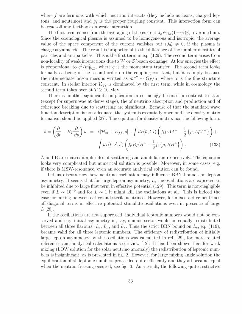
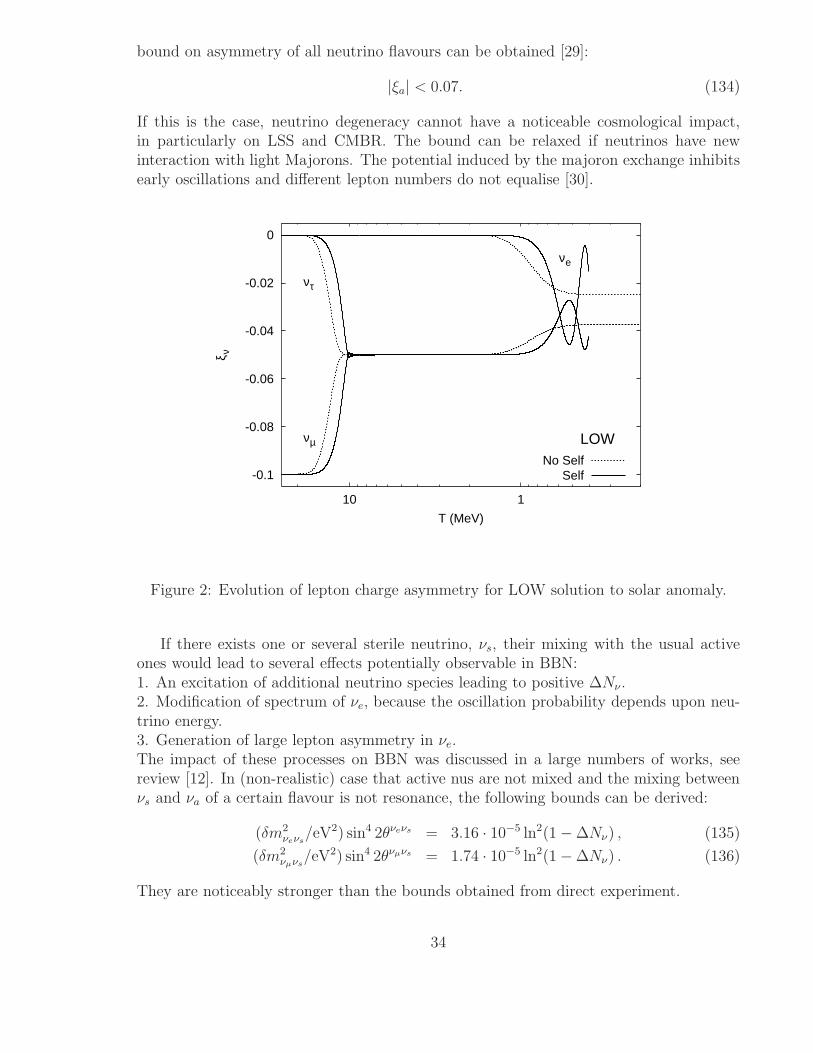
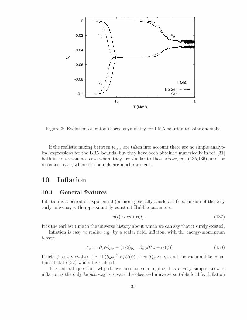


![CosmologyandNeutrinoProperties · arXiv:0803.3887v2 [hep-ph] 13 Apr 2008 CosmologyandNeutrinoProperties A.D. Dolgov ITEP, 117218, Moscow, Russia University of Ferrara and INFN, FE](https://static.documents.pub/doc/80x56/60148046e443ee6e882d3cb8/cosmologyandneutrinoproperties-arxiv08033887v2-hep-ph-13-apr-2008-cosmologyandneutrinoproperties.jpg)


