41
Introduction to Curve Estimation Wilcoxon score Density 700 800 900 1000 1100 1200 1300 0.000 0.002 0.004 0.006
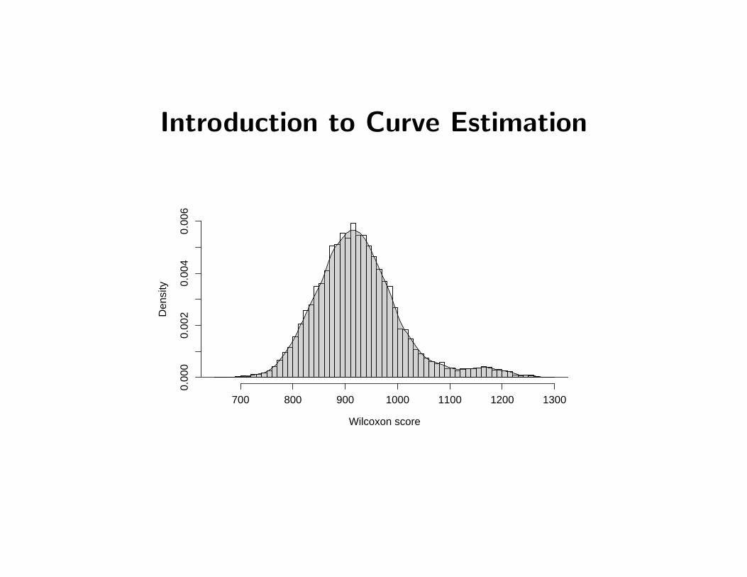
Introduction to Curve Estimation
Wilcoxon score
Den
sity
700 800 900 1000 1100 1200 1300
0.00
00.
002
0.00
40.
006
Michael E. Tarter & Micheal D. Lock
Model-Free Curve Estimation
Monographs on Statistics and Applied Probability 56
Chapman & Hall, 1993.
Chapters 1–4.
Stefanie Scheid - Introduction to Curve Estimation - August 11, 2003 1
Outline
1. Generalized representation
2. Short review on Fourier series
3. Fourier series density estimation
4. Kernel density estimation
5. Optimizing density estimates
Stefanie Scheid - Introduction to Curve Estimation - August 11, 2003 2
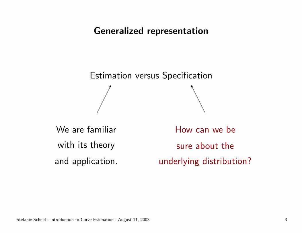
Generalized representation
Estimation versus Specification
���������
We are familiar
with its theory
and application.
AAAAAAAAK
How can we be
sure about the
underlying distribution?
Stefanie Scheid - Introduction to Curve Estimation - August 11, 2003 3
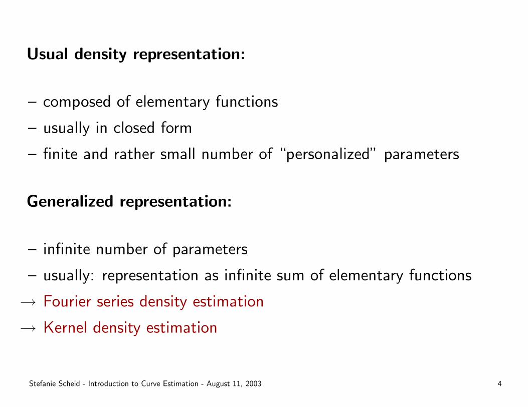
Usual density representation:
– composed of elementary functions
– usually in closed form
– finite and rather small number of “personalized” parameters
Generalized representation:
– infinite number of parameters
– usually: representation as infinite sum of elementary functions
→ Fourier series density estimation
→ Kernel density estimation
Stefanie Scheid - Introduction to Curve Estimation - August 11, 2003 4
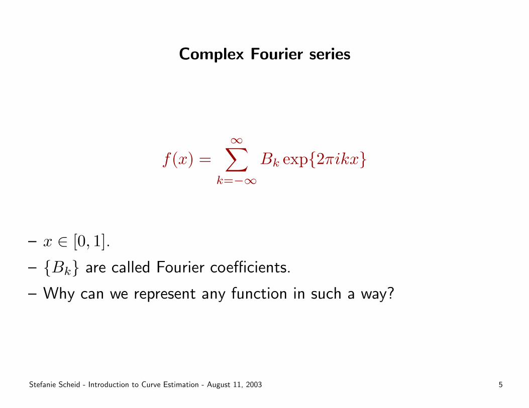
Complex Fourier series
f(x) =∞∑
k=−∞
Bk exp{2πikx}
– x ∈ [0, 1].
– {Bk} are called Fourier coefficients.
– Why can we represent any function in such a way?
Stefanie Scheid - Introduction to Curve Estimation - August 11, 2003 5
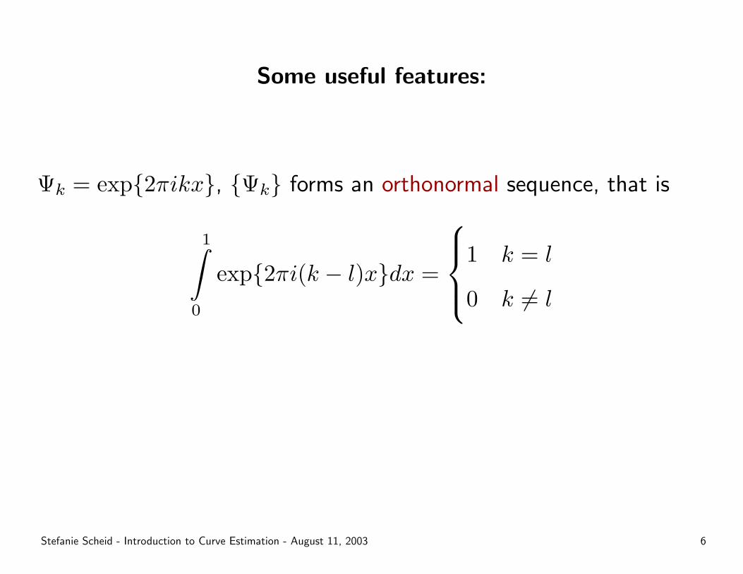
Some useful features:
Ψk = exp{2πikx}, {Ψk} forms an orthonormal sequence, that is
1∫0
exp{2πi(k − l)x}dx =
1 k = l
0 k 6= l
Stefanie Scheid - Introduction to Curve Estimation - August 11, 2003 6

{Ψk} is complete, that is
limm→∞
1∫0
f(x)−m∑
k=−m
Bk exp{2πikx}
2
dx = 0
Therefore, we can expand every function f(x), x ∈ [0, 1], in space L2
with Fourier series.
L2 function assumes that ‖f‖2 =∫|f(x)|2dx < ∞, which holds for
most of the curves we are interested in.
Stefanie Scheid - Introduction to Curve Estimation - August 11, 2003 7
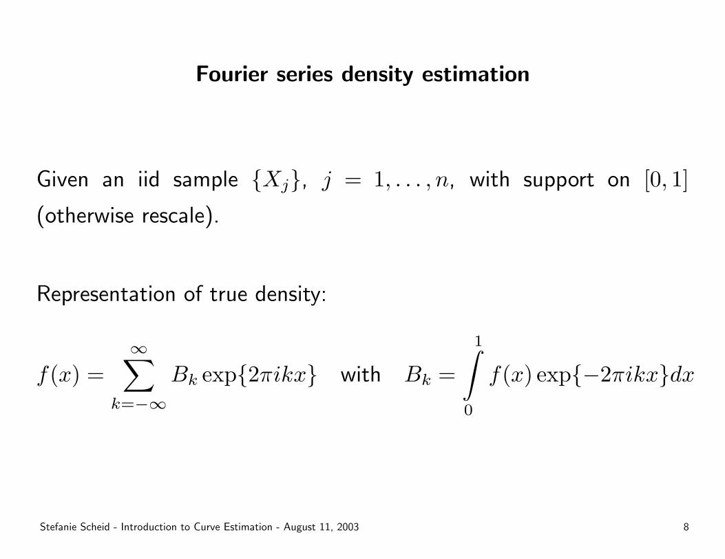
Fourier series density estimation
Given an iid sample {Xj}, j = 1, . . . , n, with support on [0, 1]
(otherwise rescale).
Representation of true density:
f(x) =∞∑
k=−∞
Bk exp{2πikx} with Bk =
1∫0
f(x) exp{−2πikx}dx
Stefanie Scheid - Introduction to Curve Estimation - August 11, 2003 8

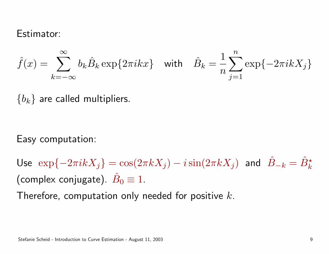
Estimator:
f̂(x) =∞∑
k=−∞
bkB̂k exp{2πikx} with B̂k =1n
n∑j=1
exp{−2πikXj}
{bk} are called multipliers.
Stefanie Scheid - Introduction to Curve Estimation - August 11, 2003 9
Estimator:
f̂(x) =∞∑
k=−∞
bkB̂k exp{2πikx} with B̂k =1n
n∑j=1
exp{−2πikXj}
{bk} are called multipliers.
Easy computation:
Use exp{−2πikXj} = cos(2πkXj)− i sin(2πkXj) and B̂−k = B̂?k
(complex conjugate). B̂0 ≡ 1.
Therefore, computation only needed for positive k.
Stefanie Scheid - Introduction to Curve Estimation - August 11, 2003 9

B̂k is unbiased estimator for Bk.
However, f̂ is usually biased because number of terms is either infinite
or unknown.
Another advantage of sample coefficients {B̂k}: Same set leads to
variety of other estimates.
That’s where multipliers come into play!
Stefanie Scheid - Introduction to Curve Estimation - August 11, 2003 10

Fourier multipliers
“Raw” density estimator:
bk =
1 |k| ≤ m
0 |k| > m⇒ f̂(x) =
m∑k=−m
B̂k exp{2πikx}
Evaluate f̂(x) in equally spaced points x ∈ [0, 1].
Stefanie Scheid - Introduction to Curve Estimation - August 11, 2003 11
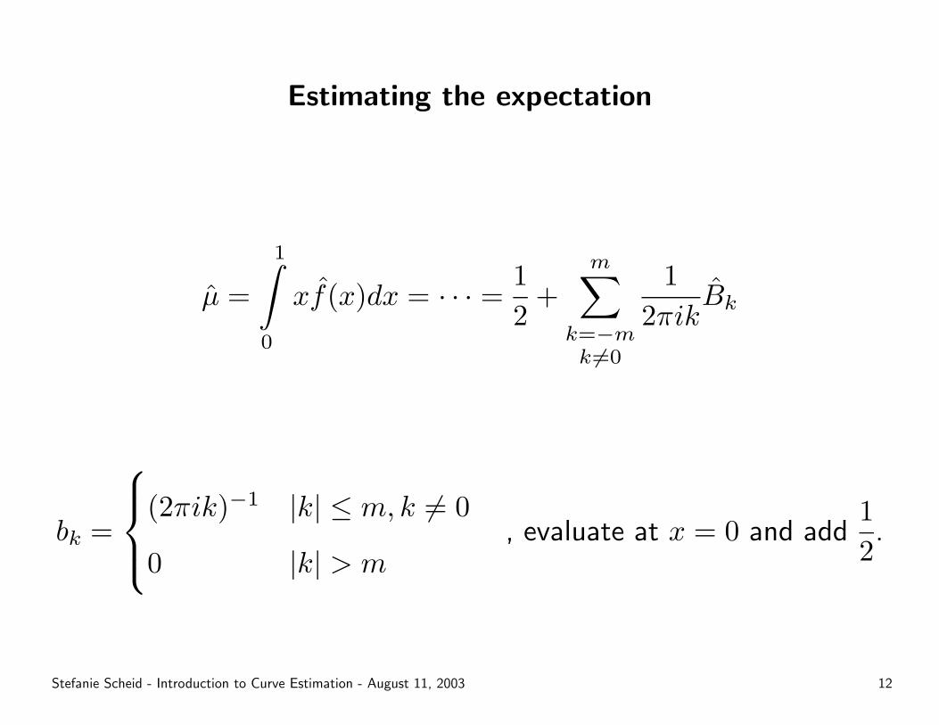
Estimating the expectation
µ̂ =
1∫0
xf̂(x)dx = · · · = 12
+m∑
k=−mk 6=0
12πik
B̂k
bk =
(2πik)−1 |k| ≤ m, k 6= 0
0 |k| > m, evaluate at x = 0 and add
12
.
Stefanie Scheid - Introduction to Curve Estimation - August 11, 2003 12

Advantages of multipliers
– Examination of various distributional features without recomputing
sample coefficients.
– Optimize the estimation procedure.
– Smoothing of estimated curve vs. higher contrast.
Some examples . . .
Stefanie Scheid - Introduction to Curve Estimation - August 11, 2003 13
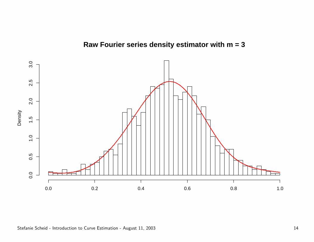
Raw Fourier series density estimator with m = 3
Den
sity
0.0 0.2 0.4 0.6 0.8 1.0
0.0
0.5
1.0
1.5
2.0
2.5
3.0
Stefanie Scheid - Introduction to Curve Estimation - August 11, 2003 14
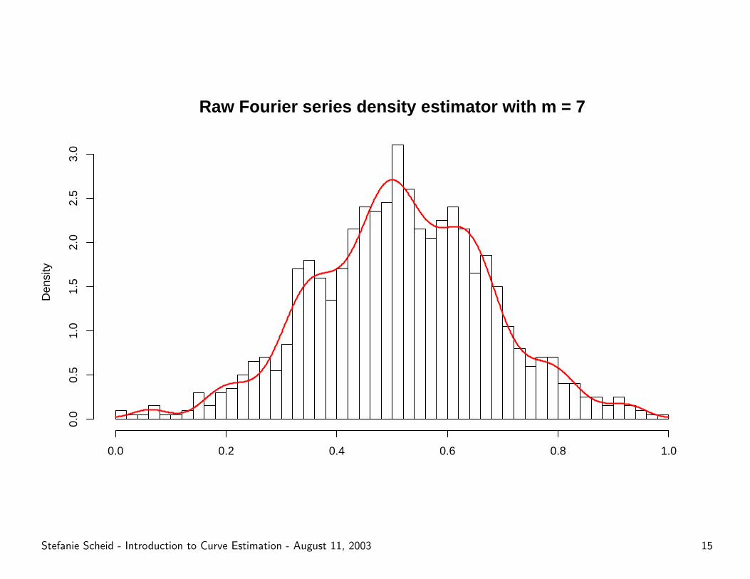
Raw Fourier series density estimator with m = 7
Den
sity
0.0 0.2 0.4 0.6 0.8 1.0
0.0
0.5
1.0
1.5
2.0
2.5
3.0
Stefanie Scheid - Introduction to Curve Estimation - August 11, 2003 15

Raw Fourier series density estimator with m = 15
Den
sity
0.0 0.2 0.4 0.6 0.8 1.0
0.0
0.5
1.0
1.5
2.0
2.5
3.0
Stefanie Scheid - Introduction to Curve Estimation - August 11, 2003 16
Kernel density estimation
Histograms are crude kernel density estimators where the kernel is a
block (rectangular shape) somehow positioned over a data point.
Stefanie Scheid - Introduction to Curve Estimation - August 11, 2003 17

Kernel density estimation
Histograms are crude kernel density estimators where the kernel is a
block (rectangular shape) somehow positioned over a data point.
Kernel estimators:
– use various shapes as kernels
– place the center of a kernel right over the data point
– spread the influence of one point with varying kernel width
⇒ contribution from each kernel is summed to overall estimate
Stefanie Scheid - Introduction to Curve Estimation - August 11, 2003 17

● ● ● ● ● ● ● ● ● ●
0 5 10 15
0.0
0.5
1.0
1.5
Gaussian kernel density estimate
● ● ● ● ● ● ● ● ● ●
Stefanie Scheid - Introduction to Curve Estimation - August 11, 2003 18
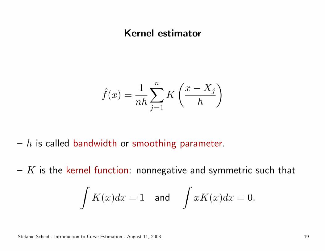
Kernel estimator
f̂(x) =1nh
n∑j=1
K
(x−Xj
h
)
– h is called bandwidth or smoothing parameter.
– K is the kernel function: nonnegative and symmetric such that∫K(x)dx = 1 and
∫xK(x)dx = 0.
Stefanie Scheid - Introduction to Curve Estimation - August 11, 2003 19
– Under mild conditions (h must decrease with increasing n) the
kernel estimate converges in probability to the true density.
– Choice of kernel function usually depends on computational criteria.
– Choice of bandwidth is more important (see literature on “Kernel
Smoothing”).
Stefanie Scheid - Introduction to Curve Estimation - August 11, 2003 20

Some kernel functions
−4 −2 0 2 4
0.0
0.1
0.2
0.3
0.4
Gauss
−2 −1 0 1 2
0.0
0.2
0.4
0.6
0.8
1.0
Triangular
−3 −2 −1 0 1 2 3
0.00
0.05
0.10
0.15
0.20
0.25
0.30
Epanechnikov
K(y) =3(1− y2/5)
4√
5, |y| ≤
√5
Stefanie Scheid - Introduction to Curve Estimation - August 11, 2003 21

Duality of Fourier series and kernel methodology
f̂(x) =∑k
bkB̂k exp{2πikx}
=1n
n∑j=1
∑k
bk exp{2πik(x−Xj)}
With h = 1:
K(x) =∑k
bk exp{2πikx}
Stefanie Scheid - Introduction to Curve Estimation - August 11, 2003 22
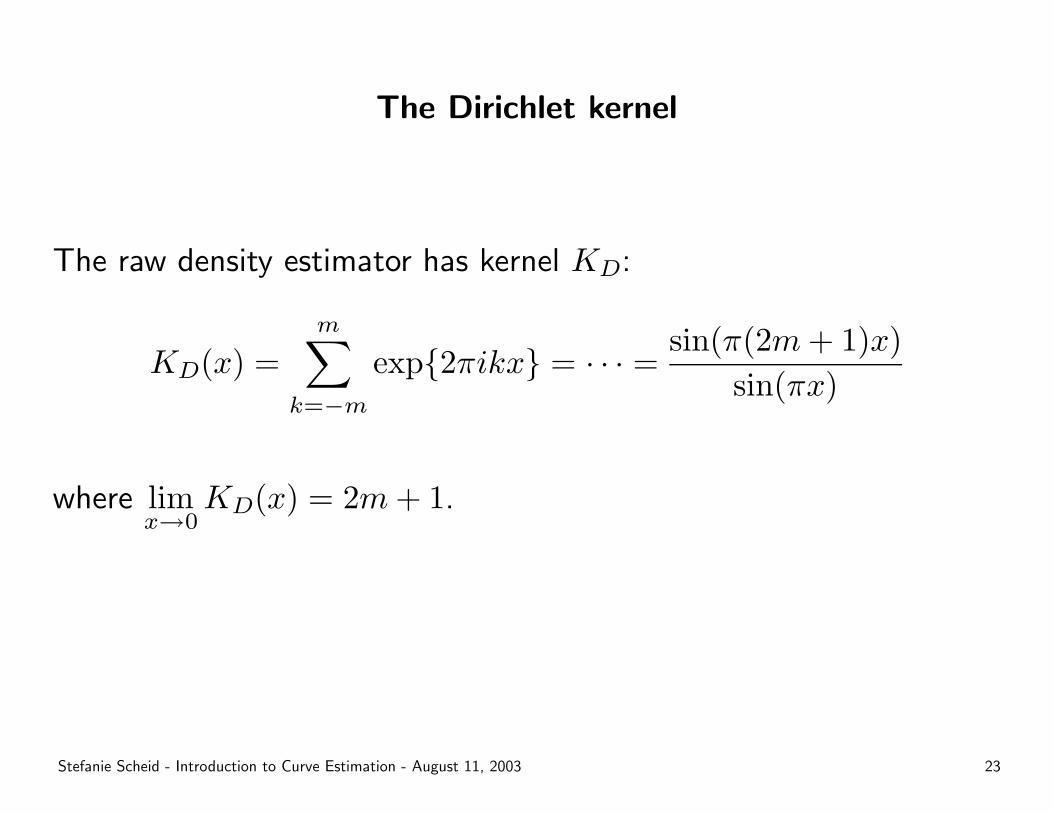
The Dirichlet kernel
The raw density estimator has kernel KD:
KD(x) =m∑
k=−m
exp{2πikx} = · · · = sin(π(2m+ 1)x)sin(πx)
where limx→0
KD(x) = 2m+ 1.
Stefanie Scheid - Introduction to Curve Estimation - August 11, 2003 23

Dirichlet kernels
−0.4 −0.2 0.0 0.2 0.4
−10
010
2030
Dirichlet with m = 4
−0.4 −0.2 0.0 0.2 0.4
−10
010
2030
Dirichlet with m = 8
−0.4 −0.2 0.0 0.2 0.4
−10
010
2030
Dirichlet with m = 12
Stefanie Scheid - Introduction to Curve Estimation - August 11, 2003 24
Differences between kernel and Fourier representation
– Fourier estimates are restricted to finite intervals while some kernels
are not.
– As Dirichlet kernel shows, kernel estimates can result in negative
values if the kernel function takes on negative values.
Stefanie Scheid - Introduction to Curve Estimation - August 11, 2003 25

– Kernel: K controls shape, h controls spread of kernel.
Two-step strategy: Select kernel function and choose data-
dependent smoothing parameter.
– Fourier: m controls both shape and spread.
Goodness-of-fit can be governed by entire multiplier sequence.
Stefanie Scheid - Introduction to Curve Estimation - August 11, 2003 26

Optimizing density estimates
Optimization with regard to weighted mean integrated square error
(MISE):
J(f̂ , f, w) = E
1∫0
(f(x)− f̂(x)
)2
w(x)dx.
w(x) is nonnegative weight function to emphasize estimation over
subregions. First consider optimization with w(x) ≡ 1.
Stefanie Scheid - Introduction to Curve Estimation - August 11, 2003 27
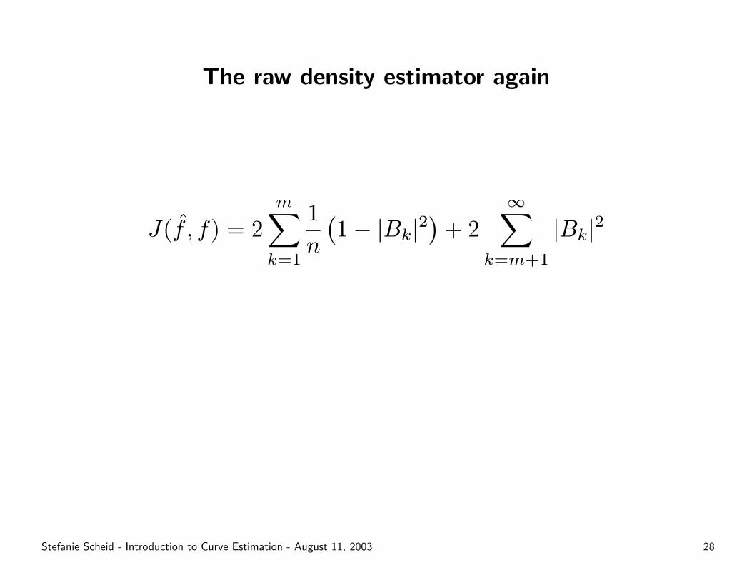
The raw density estimator again
J(f̂ , f) = 2m∑k=1
1n
(1− |Bk|2
)+ 2
∞∑k=m+1
|Bk|2
Stefanie Scheid - Introduction to Curve Estimation - August 11, 2003 28
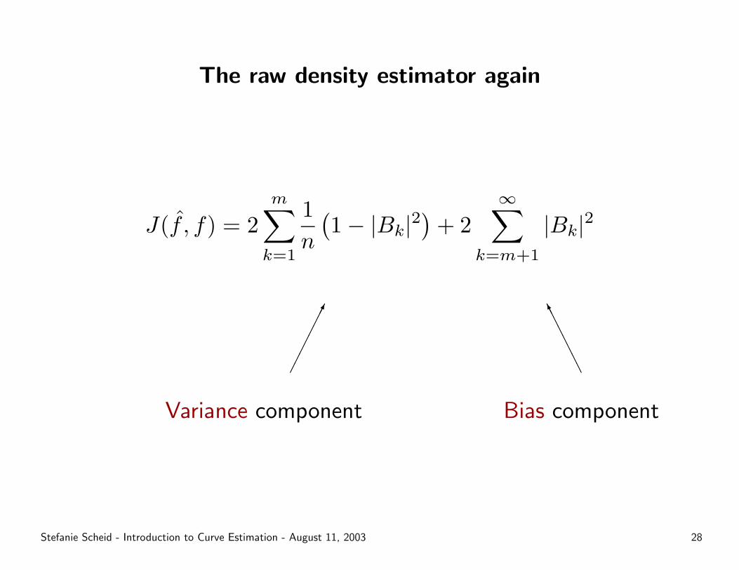
The raw density estimator again
J(f̂ , f) = 2m∑k=1
1n
(1− |Bk|2
)+ 2
∞∑k=m+1
|Bk|2
���������
Variance component
AAAAAAAAK
Bias component
Stefanie Scheid - Introduction to Curve Estimation - August 11, 2003 28
Single term stopping rule
– Estimate ∆Js = J(f̂s, f)−J(f̂s−1, f), gain of including sth Fourier
coefficient. MISE is decreased if ∆Js is negative.
– Include terms only if their inclusion results in negative difference.
Multiple testing problem!
– Inclusion of higher-order terms results in rough estimate.
– Suggestions: Stop after t successive nonnegative inclusions. Choice
of t is data/curve dependent.
Stefanie Scheid - Introduction to Curve Estimation - August 11, 2003 29
Other stopping rules
– Different considerations about estimating MISE lead to various
optimization concepts.
– Not at all generally superior to single term rule. Depends on curve
features.
Stefanie Scheid - Introduction to Curve Estimation - August 11, 2003 30
Multiplier sequences
– So far: “raw” estimate with bk = 1 or bk = 0.
– Now allow {bk} to be sequence tending to zero with increasing k.
– Concepts depend again on considerations about MISE.
– Question of advisable stopping rule remains.
Stefanie Scheid - Introduction to Curve Estimation - August 11, 2003 31
Two-step strategy with multiplier sequence
1. Estimate with raw estimator and one of former stopping rules.
2. Applying a multiplier sequence to the remaining terms will always
improve the estimate.
Stefanie Scheid - Introduction to Curve Estimation - August 11, 2003 32

Weighted MISE
J(f̂ , f, w) = E
1∫0
(f(x)− f̂(x)
)2
w(x)dx.
– Weight functions w(x) emphasize subregions of support interval
(e.g. left or right tails).
– Turns out that unweighted MISE leads to great accuracy in regions
with high density.
⇒ Weighting will improve estimate when other regions are of interest.
Stefanie Scheid - Introduction to Curve Estimation - August 11, 2003 33
Data transformation
– Data needs rescaling to [0, 1]. Always possible:Xj−min(X)
max(X)−min(X)
– Next approach: Transform data in nonlinear manner to emphasize
subregions.
Stefanie Scheid - Introduction to Curve Estimation - August 11, 2003 34
Data transformation
– Data needs rescaling to [0, 1]. Always possible:Xj−min(X)
max(X)−min(X)
– Next approach: Transform data in nonlinear manner to emphasize
subregions.
– Let G : [a, b] → [0, 1] be strictly increasing one-to-one function
with g(x) = dG(x)dx .
⇒ Ψk(G(x)) = exp{2πikG(x)} is orthonormal on [a, b] with respect
to weight g(x).
Stefanie Scheid - Introduction to Curve Estimation - August 11, 2003 34
Transformation and optimization
– Data transformation with G(x) is equivalent to weighted MISE
with w(x) = 1/g(x).
– Only difference to unweighted MISE: Computation of Fourier
coefficients involves application of G(x).
⇒ Strategy: Transform data, optimize with unweigthed procedures,
retransform.
Most efficient: Transform data to unimodal symmetric distribution.
Stefanie Scheid - Introduction to Curve Estimation - August 11, 2003 35
Application to gene expression data
– Problem: Fitting two distributions to another by removing a
minimal number of data points.
– Idea: Estimate the two densities in an optimal manner. Remove
points until goodness-of-fit is high with regard to modified MISE.
Stefanie Scheid - Introduction to Curve Estimation - August 11, 2003 36


