AbstractThis course presents an introduction to CAGD—Computer-Aided GeometricDesign. The mathematical tools required to create well-behaved curves andsurfaces are covered, together with efficient algorithms for their implementation.Topics covered include basis functions, Bézier curves, B-splines, and surfacepatches.
3
Table of Contents
Topic Page
Introduction to CAGD 10
Preliminary Mathematics 18
The Bézier Curve 32
Blossoms 53
The B-Spline Curve 64
Surfaces 76
Bibliography 87
Tom Berryhill
These items are clickable.
4
Course Contributors
Dr. Alyn P. RockwoodAlyn P. Rockwood completed B.S. and M.S. degrees in mathematics at BrighamYoung University and a Ph.D. at the Dept. of Applied Mathematics andTheoretical Physics of Cambridge University, Cambridge, England. He worked inindustrial research for 13 years, including supervisory and research positions atEvans and Sutherland Computer Corp. and Silicon Graphics, Inc. He wasinvolved in flight simulation, CAD/CAM and surface rendering projects at thesecompanies.
Currently, he is on the computer science faculty at Arizona State University. Hisinterests include computer graphics, scientific visualization and computer aidedgeometric design. He has several patents and many publications in these fields.
Peter ChambersPeter Chambers received his B.Sc. from the University of Exeter, England, andhis M.S. from Arizona State University. Peter is an Engineering Fellow in theAdvanced Multimedia Group at VLSI Technology, Tempe, Arizona. His areas ofinterest at VLSI include circuit design, computer architectures, and peripheralinterfaces for personal computers.
Peter has architected and designed numerous products, including theInput/Output systems for minicomputers, and many large integrated circuits.Peter's other interests include high level hardware description languages,techniques for robust design, and interface performance analysis.
Peter's involvement with Arizona State University includes research on texturingmethods in computer graphics and interactive learning tools. His most recentpublication is Interactive Curves and Surfaces, in collaboration with AlynRockwood, upon which these course notes are based.
5
Dr. Hans HagenHans Hagen is a professor of computer science at the University ofKaiserslautern, Germany. His research centers on geometric modeling andscientific visualization.
Dr. Hagen received his B.A. and his M.S. from the University of Freiburg and hisPh.D. from the University of Dortmund. Before moving to Kaiserslautern he heldfaculty positions at the University of Braunschweig and at Arizona StateUniversity. He is one of the current directors at the Dagstuhl Conference andResearch Center.
Dr. Hagen is on the editorial board of Computer Aided Geometric Design,Transactions on Visualization and Computer Graphics, Computer Aided Design,Computing, and Surveys on Mathematics for Industry.
Thomas McInerneyThomas McInerney writes code for Apple Computer during his summers. Hisinterests are in computer graphics and computer networks. He is completing hisB.S. in Computer Science from Arizona State University. He is also writing theJava version of the curves and surfaces book with Alyn Rockwood andPeter Chambers.
6
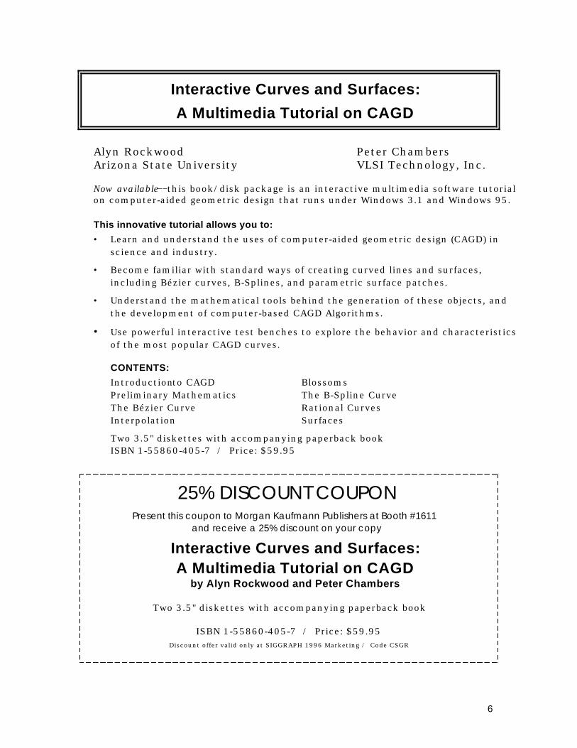
Interactive Curves and Surfaces:
A Multimedia Tutorial on CAGD
Alyn Rockwood Peter ChambersArizona State University VLSI Technology, Inc.
Now available−−this book/disk package is an interactive multimedia software tutorialon computer-aided geometric design that runs under Windows 3.1 and Windows 95.
This innovative tutorial allows you to:• Learn and understand the uses of computer-aided geometric design (CAGD) in
science and industry.
• Become familiar with standard ways of creating curved lines and surfaces,including Bézier curves, B-Splines, and parametric surface patches.
• Understand the mathematical tools behind the generation of these objects, andthe development of computer-based CAGD Algorithms.
• Use powerful interactive test benches to explore the behavior and characteristicsof the most popular CAGD curves.
CONTENTS:Introduction to CAGD BlossomsPreliminary Mathematics The B-Spline CurveThe Bézier Curve Rational CurvesInterpolation Surfaces
Two 3.5" diskettes with accompanying paperback bookISBN 1-55860-405-7 / Price: $59.95
25% DISCOUNT COUPONPresent this coupon to Morgan Kaufmann Publishers at Booth #1611
and receive a 25% discount on your copy
Interactive Curves and Surfaces:A Multimedia Tutorial on CAGD
by Alyn Rockwood and Peter Chambers
Two 3.5" diskettes with accompanying paperback book
ISBN 1-55860-405-7 / Price: $59.95Discount offer valid only at SIGGRAPH 1996 Marketing / Code CSGR
7
Contact Information
Alyn RockwoodDr. Alyn P. RockwoodDepartment of Computer ScienceArizona State UniversityTempeArizona 85287
AcknowledgmentsAlyn Rockwood and Peter Chambers wish to thank:
Mike Morgan and Marilyn Uffner Alan at Morgan Kaufman, for making theInteractive Curves and Surfaces project possible.
Spencer Thomas, Jim Miller, Aristides Requicha, and Jules Bloomenthal, fortheir excellent comments and ideas.
Shara-Dawn Simon, for her diligent proof-reading, and the significantimprovements in layout and flow she suggested.
Professor Don Evans, director of the Center of Innovation in EngineeringEducation, of the College of Engineering and Applied Science, Arizona StateUniversity, for support and encouragement.
The authors also appreciate the sponsorship of the US/Hungarian Science andTechnology Joint Fund, in cooperation with Arizona State University, project396.
10
Topic 1
Introduction toCAGD
11
Topic 1: Introduction to CAGD
In this topic, you will:
• Learn what CAGD is about.
• Learn some of the history of CAGD.
• See some typical applications of CAGD tools.
What CAGD is All About
Computer-Aided Geometric Design is a new field that initially developed tobring the advantages of computers to industries such as:
• Automotive
• Aerospace
• Shipbuilding
CAGD expanded rapidly and now pervades many areas, from pharmaceuticaldesign to animation. We are surrounded by products that are first visualizedon a computer. These products are modified and refined entirely within thecomputer; when the product enters production, the tools and dies areproduced directly from the geometry stored in the computer. This process isknown as virtual prototyping.
(c) 1995 Autodesk, Inc. This image was provided courtesy of Autodesk, Inc.
12
Computer visualizations of new products reduce the design cycle by easingthe process of design modification and tool production.
CAGD is based on the creation of curves and surfaces, and is accuratelydescribed as curve and surface modeling. Using CAGD tools with elaborateuser interfaces, designers create and refine their ideas to produce complexresults. They combine large numbers of curve and surface segments to realizetheir ideas. However, the individual segments they use are relatively simple,and it is at this level that the study of CAGD is concentrated.
A Design Challenge: The Need for CAGD
When creating products and artwork, designers face tasks such as this:
You are given two points in a plane and two directions associated with thepoints. Find the curve that passes through the points that is tangent to the givendirections:
This is a simple task for anyone with a pencil and paper who is familiar withparametric forms, the types of curves used in CAGD.
CAGD produces tools are meant to be:
• Intuitive
• Simple to use
Sometimes the mathematics underlying the tools becomes quite sophisticated,yet the result is meant to be easily understood and geometrically intuitive.
13
The technical person often benefits from these intuitive and visually related toolswhen considering deeper mathematical problems. The geometry of CAGD isvery amenable to visual demonstration.
CAGD: From Points to Teapots
There is a natural progression of the geometry behind CAGD. With smallincremental steps it is possible to describe complex objects in terms of simpleprimitives, such as points and lines.
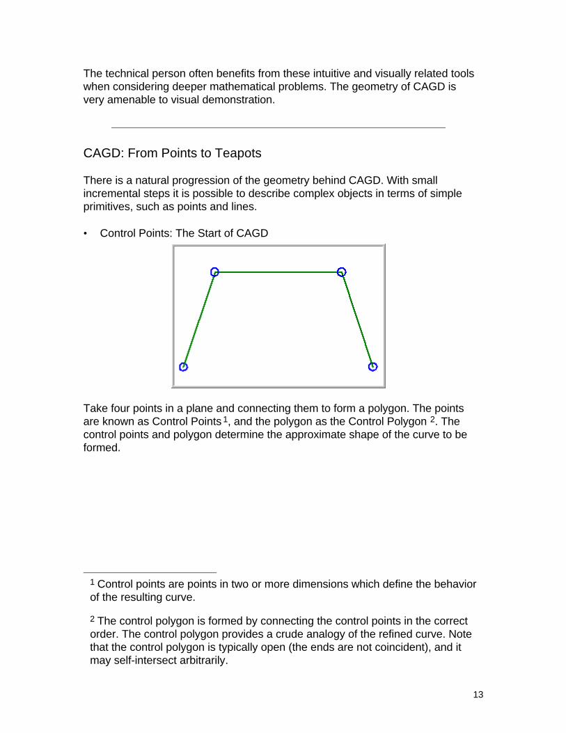
• Control Points: The Start of CAGD
Take four points in a plane and connecting them to form a polygon. The pointsare known as Control Points 1, and the polygon as the Control Polygon 2. Thecontrol points and polygon determine the approximate shape of the curve to beformed.
1 Control points are points in two or more dimensions which define the behaviorof the resulting curve.
2 The control polygon is formed by connecting the control points in the correctorder. The control polygon provides a crude analogy of the refined curve. Notethat the control polygon is typically open (the ends are not coincident), and itmay self-intersect arbitrarily.
14
• A CAGD Favorite: The Bézier Curve
A special curve known as the Bézier Curve 3 may be generated by the controlpoints. Note that while the curve passes through the end points, it only comesclose to the other points.
• Three-Dimensional Control Polygons for Surfaces (Control Meshes)
Bézier curves behave just as well in three dimensions as in two. This figureshows the control polygons for a three-dimensional object consisting of Bézierpatches4.
3 The Bézier curve, named after the French researcher Pierre Bézier, is asimple and useful CAGD curve. It is a very well behaved curve with usefulproperties, as you will discover in Topic 3, The Bézier Curve.4 A Bézier patch is a three-dimensional extension of a Bézier curve. It is formedby extruding a Bézier curve through space to form a surface.
15
• Three-Dimensional Wireframe Model
When the Bézier curves are created and connected in three dimensions, awireframe model of the object is produced.
• Three-Dimensional Shaded Object
If the surface produced by the three-dimensional Bézier patches is illuminatedand shaded, an object with a realistic appearance results. The Utah teapot, ondisplay at the Boston Museum of Computer History, is a classic in CAGD andcomputer graphics.
16
The History of CAGD
Computer Aided Geometric Design has mathematical roots that stretch back toEuclid and Descartes. Its practical application began with automatedmachinery to compute, draft, and manufacture objects with freeform surfaces.Production pressures in the aircraft industry during World War II stimulatedmany new devices to enhance and accelerate design and manufacturing. Forexample, in 1944 Liming designed fuselage spars with a "super-elliptic"method that could be implemented with an electro-mechanical calculator.
Shipbuilders also became interested in CAGD early on. One example of theirmotivation may sound whimsical but was a serious impediment to ship design.The only place large enough to draw full scale plans for a ship was in the loftof the shipbuilders dry-dock. The huge drawings would warp and shrink in themoist air, causing very real manufacturing problems.
Computers provided the greatest stimulus because of their power to enablenew ideas. In 1963, Ferguson developed one of the first surface patch systemsby which individual curvilinear patches are joined smoothly to create thesurface "quilt." He also introduced the notion of parametrically definedsurfaces which has become the standard because it provides freedom from anarbitrarily fixed coordinate system. Vertical tangent vectors can be defined bydifferentiation, for instance, which is not possible in explicit Cartesian form.
In the mid 1960's automotive companies became involved in CAGD, as a wayto drive milling machines. Car bodies were designed by artists using claymodels. Painstaking measurements produced data that could drive numericallycontrolled milling machines to produce stamp molds. The initial use of CAGDwas to represent the data as a smooth surface for numerical control. It soonbecame apparent that the surfaces could be used for the design.
In 1971, Pierre Bézier reformulated Ferguson's ideas so that a draftsmanwithout any extensive mathematical training could design a surface. Bezier'ssystem, UNISURF, was used by Renault and became a milestone in thedevelopment of CAGD. It epitomized the difference between surface fitting andsurface design. The purpose of design was to provide the draftsman, who hadstrong intuition about shape but limited mathematical training, computer toolsthat empowered him or her to use the sophisticated mathematics of surfacerepresentation.
In the meantime, the mathematical underpinnings of CAGD continued toadvance. de Casteljau examined triangular patches and developed evaluationtechniques. Coons [Coons64] unified much of the previous work into a generalscheme which became the basis of the early modeler PDGS made by Ford. AtGeneral Motors in 1974, Gordon and Riesenfeld exploited the properties of B-spline curves and surfaces for design.
Driven primarily by the automotive, shipbuilding and aerospace industries,both the mathematics of CAGD and the designer interface tools continued to
17
improve through the 1970's. The first CAGD conference was organized byBarnhill and Riesenfeld in 1974, where the term "CAGD" was first used[Barnhill74].
In the 1980's, the power and versatility of computer-aided designing seemedsuddenly to be discovered by anyone who had a freeform geometric surfaceapplication. Industrial designers were smitten with the power of computerdesign, and many commercial modelers become the basis of severalsubstantial applications, including: CATIA, EUCLID, STRIM, ANVIL, andGEOMOD. Geoscience used CAGD methods to represent seismic horizons;computer graphics designers modeled their objects with surfaces, as didmolecule designers for pharmaceuticals. Architects discovered them, wordprocessing and drafting programs based their interface protocols on freeformcurves (PostScript5), and even moviemakers discovered the power ofanimating with such surfaces, beginning with TRON, continuing throughJurassic Park6, and beyond.
What has Been Accomplished in this Topic
The ideas and principles behind CAGD have been introduced, together with theclassic example of surface patch use, the Utah teapot. The short but significanthistory of CAGD has been summarized.
5 PostScript is a proprietary page-description language used by typesetters todefine elements of printed text, including letter outlines, text layout, andgraphical images.
6 Jurassic Park made extensive use of CAGD and computer graphics tovisualize animated objects.
18
Topic 2
PreliminaryMathematics
19
Topic 2: Preliminary Mathematics
In this topic, you will learn:
• The basic math needed for the rest of the book.
• An overview of parametric forms: a convenient way of describing curvesand surfaces.
• An illustration of linear interpolation, one of the most fundamentalconcepts in CAGD.
• The idea of continuity, to ensure that curves and surfaces join togethersmoothly.
The Mathematics of CAGD
CAGD treats points, lines, and surfaces as mathematical objects, describedgeometrically in two- or three-dimensional space.
This book develops the mathematics in a step-by-step fashion, and does notdemand a rigorous mathematical background. It is recommended that thereader be familiar with the following topics:
• Geometry of points, lines, and planes.
• Equations in parametric form.
• Basic calculus.
20
Parametric Forms
CAGD relies on parametric forms to describe curves and surfaces. Manystudents of CAGD do not initially appreciate the subtlety and importance ofthis form. If you are confident with parametric forms then you may skip thissection.
The Parametric Curve
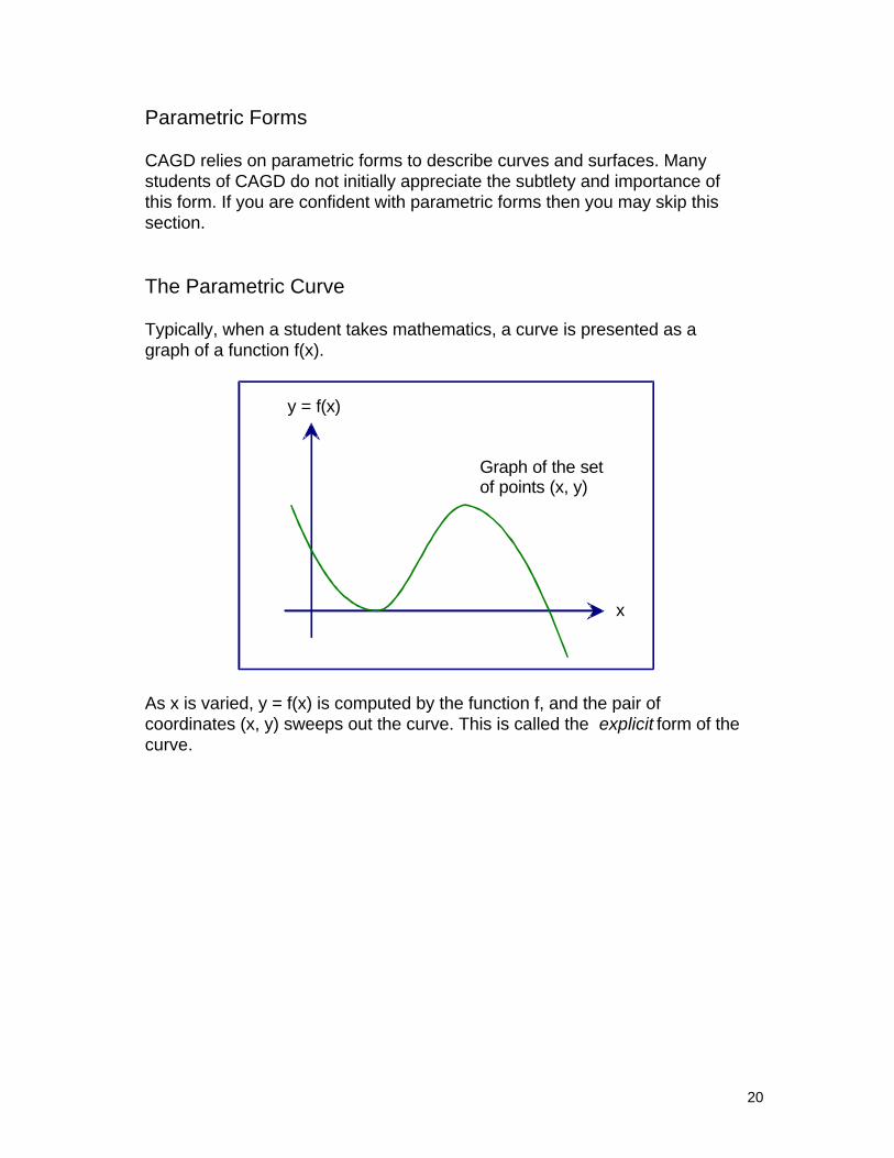
Typically, when a student takes mathematics, a curve is presented as agraph of a function f(x).
Graph of the setof points (x, y)
x
y = f(x)
As x is varied, y = f(x) is computed by the function f, and the pair ofcoordinates (x, y) sweeps out the curve. This is called the explicit form of thecurve.
21
From a design standpoint the explicit form is deficient in several ways:
• Single-Valued
x
y = f(x)The circle has twovalues along this line
The curve is single-valued along any line parallel to the y axis. For example,only parts of the circle may be defined explicitly.
• Infinite Slope
x
y = f(x)The circle has twopoints with infinite slope
An explicit curve cannot have infinite slope; the derivative f' (x) is not definedparallel to the y axis. Hence there are two points on the circle that cannot bedefined.
• Transformation Problems
Any transformation, such as rotation or shear, may cause an explicit curve toviolate the two points above.
22
The parametric form of a curve is not subject to these limitations. Moreover, itprovides a method, known as parameterization 1, that defines motion on thecurve. Motion on the curve refers to the way that the point (x, y) traces outthe curve.
Defining the Parametric Curve
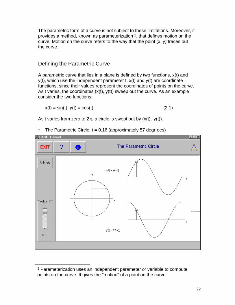
A parametric curve that lies in a plane is defined by two functions, x(t) andy(t), which use the independent parameter t. x(t) and y(t) are coordinatefunctions, since their values represent the coordinates of points on the curve.As t varies, the coordinates (x(t), y(t)) sweep out the curve. As an exampleconsider the two functions:
x(t) = sin(t), y(t) = cos(t). (2.1)
As t varies from zero to 2π, a circle is swept out by (x(t), y(t)).
• The Parametric Circle: t = 0.16 (approximately 57 degr ees)
1 Parameterization uses an independent parameter or variable to computepoints on the curve. It gives the "motion" of a point on the curve.
23
CAGD deals primarily with polynomial 2 or rational functions 3, nottrigonometric functions as shown in the examples above. For example, thecircle can also be given by allowing t to vary from -infinity to +infinity in thefollowing functions:
( ) ( ) ( ) ( )( )x t
tt
y tt
t=
+=
−
+2
1
1
12
2
2, . (2.2)
As an exercise, verify for yourself that the functions in equation 2.2 doindeed generate a circle. Plot points (x(t), y(t)) or write a program to do thisfor you.
Both equation 2.1 and equation 2.2 yield circles, so how do they differ? It isthe parameterization. The motion of the point (x(t), y(t)) is different, even ifthe paths (the circles) are the same.
A good physical model for parametric curves is that of a moving particle 4.The parameter t represents time. At any time t the position of the particle is(x(t), y(t)). Two paths (curves) may be identical even though the motion(parameterization) is different.
Parametric curves are not constrained to be single-valued along any line(recall the single-valued deficiency of the explicit form), and the slope of aparametric curve segment may be defined vertically. The slope is given bythe tangent line at any point, computed by finding the derivative vector (x'(t),y'(t)) at any point t. This vector determines the speed at which the pointtraces out the curve as t changes.
Curves defined by points whose speed may drop to zero do cause problemsthat will be considered later under the discussion of continuity.
2 A polynomial is a function of the form:
( )p t a a t a t a tnn= + + + +0 1 2
2 ... , . where the a are scalars or vectorsi
3 A rational function is made by dividing one polynomial by another, forexample:
( )r t t t tt
= − + +−
1 2 31 2
3 4
2 .
A rational function may contain vector coefficients only within the numerator.
4 As the parameter t changes, the coordinate point (x(t), y(t)) traces the curve.This point can be thought of as a particle that moves under the influence ofchanges in the value of the parameter t.
24
Consider the parametric curve given by these two coordinate functions:
( )( )
x t t t t
y t t t
= − +
= −
6 9 4
4 3
2 3
3 2
,
.(2.3)
• Bézier tangent demonstration
The illustration above demonstrates the following for this parametric curve,as t varies between 0 and 1:
• The parameter t moves the point (x(t), y(t)) along the path of the curve.
• The point's speed varies as t varies. The speed is higher at the ends ofthe curve.
• The derivative vector changes in length, reflecting the variation in thespeed of the point.
• In the demonstration, the curve crosses itself, which can easily happenwith parametric curves.
A convenient notation for equation 2.3 is:
25
( ) ( )( )f t
x ty t
t t t=
=
+
−−
+
60
93
44
2 3. (2.4)
Equations 2.3 and 2.4 are the same. We simply save on notation by writingthe basis functions5 only once, which are then multiplied by the appropriatevectors. When a vector is multiplied by a scalar, each coordinate in thevector is individually multiplied by the scalar.
In general, a parametric polynomial is written as:
( )f a a a at t t tnn= + + +0 1 2
2 ... . (2.5)
where f(t) is a vector-valued function, and the a's are vectors. The vectorsare not restricted to two dimensions. The a's might be vectors of threedimensions, for instance. In this case the function f(t) would have threecoordinate functions x(t), y(t), and z(t). The curve would be a curve in space,and the derivative f'(t) would be given by the vector of the derivativecoordinate functions (x'(t), y'(t), z'(t)).
The general case described by equation 2.5 includes a constant term ( a0),which the example given by equations 2.3 and 2.4 does not have.
5 Here, the basis functions are 1, t and t, , .t2 3
The coefficient for the basis function "1" is 00
.
26
The Parametric Surface
As with curves, it is typical for the reader to have encountered surfacesexplicitly as z = f(x, y). Often called elevation surfaces or terrain, the height zis given at a point on the plane by computing f(x, y). Such a surface definitionshares the same flaws mentioned previously for curves:
• They must be single-valued for any point on the plane.
• They cannot have vertical tangent planes.
• Transformations may cause the above two difficulties.
The parametric form of the surface corrects these problems. In order todefine a parametric surface, it is best to first define a parametric curve, andthen sweep the curve through space to define the surface.
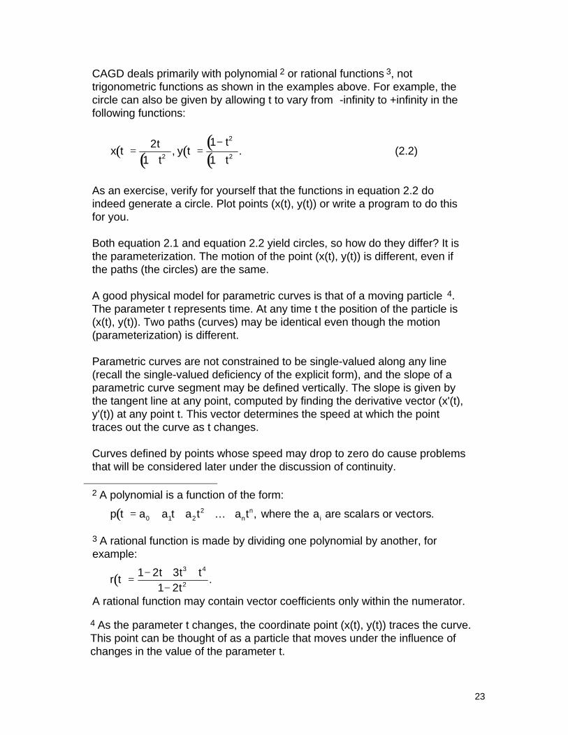
Consider a planar curve given by:
( )( )
x t t
y t t t
= −
= −
2 2
2 2 2
,
.(2.6)
Or in vector form,
( )( )
x ty t
t t
=
+
−
+
−
20
22
02
2. (2.7)
The curve given by x(t) and y(t) looks like this:
x(t) = 2 - 2ty(t) = 2t-2t
(x(t), y(t))
x
y
2
2
0.5
00
Here, the parameter t is limited to the range 0 to 1.
The curve becomes a surface in three dimensions if another parameter s andanother coordinate function z are added. Consider, for instance:
27
( )( )( )
x s t t
y s t t t
z s t s
, ,
, ,
, .
= −
= −
=
2 2
2 2 2 (2.8)
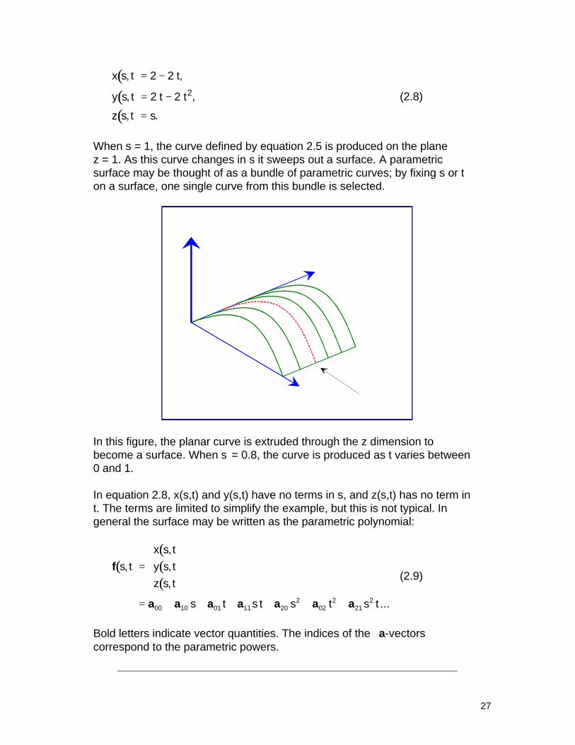
When s = 1, the curve defined by equation 2.5 is produced on the planez = 1. As this curve changes in s it sweeps out a surface. A parametricsurface may be thought of as a bundle of parametric curves; by fixing s or ton a surface, one single curve from this bundle is selected.
In this figure, the planar curve is extruded through the z dimension tobecome a surface. When s = 0.8, the curve is produced as t varies between0 and 1.
In equation 2.8, x(s,t) and y(s,t) have no terms in s, and z(s,t) has no term int. The terms are limited to simplify the example, but this is not typical. Ingeneral the surface may be written as the parametric polynomial:
( )( )( )( )
f
a a a a a a a
s tx s ty s tz s t
s t s t s t s t
,,,,
...
=
= + + + + + +00 10 01 11 20 02 212 2 2
(2.9)
Bold letters indicate vector quantities. The indices of the a-vectorscorrespond to the parametric powers.
28
Continuity
The notion of continuity 6 was developed for explicit functions to describewhen a curve does not break or tear. If it meets these conditions, it isdescribed as C0. C0 continuity is defined by the popular description: "A curveis continuous if it can be drawn without lifting the pencil from the paper."
If the derivative curve is also continuous, then the curve is first-orderdifferentiable and is said to be C 1 continuous. Extending this idea, it is saidthat a curve is Ck differentiable if the kth derivative curve is continuous.
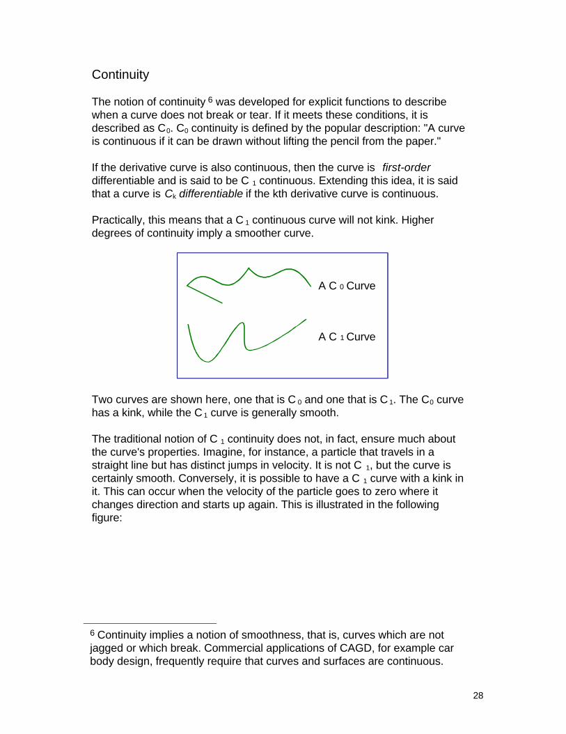
Practically, this means that a C 1 continuous curve will not kink. Higherdegrees of continuity imply a smoother curve.
A C 0 Curve
A C 1 Curve
Two curves are shown here, one that is C 0 and one that is C 1. The C0 curvehas a kink, while the C 1 curve is generally smooth.
The traditional notion of C 1 continuity does not, in fact, ensure much aboutthe curve's properties. Imagine, for instance, a particle that travels in astraight line but has distinct jumps in velocity. It is not C 1, but the curve iscertainly smooth. Conversely, it is possible to have a C 1 curve with a kink init. This can occur when the velocity of the particle goes to zero where itchanges direction and starts up again. This is illustrated in the followingfigure:
6 Continuity implies a notion of smoothness, that is, curves which are notjagged or which break. Commercial applications of CAGD, for example carbody design, frequently require that curves and surfaces are continuous.
29
Mathematicians have developed the concept of a manifold as a new way ofdescribing continuity. In CAGD there is a simpler concept to achieve thesame end. It is the idea of geometric continuity 7. If a curve is C0, it is G0
continuous. If a curve's tangent direction changes continuously then it is G 1
continuous. Its magnitude may jump discontinuously but the curve is still G 1.Hence a particle traveling at erratically changing speeds may still trace out asmooth curve if its direction changes smoothly. This is illustrated in thefollowing figure:
Sudden changein tangent length
If a C1 curve has kinks because its derivative goes to zero at a point, thenthis curve will not be G 1, since the tangent direction changes discontinuouslyat the kink. Hence the notion of geometric continuity provides a useful way tounderstand the smoothness of a curve or surface.
7 Geometric continuity introduces a notation that immediately tells the designerwhether or not the curve is smooth.
30
Linear Interpolation
Given two points in space, a line can be defined that passes through themboth in parametric form:
( ) ( )l b bt t t= − +1 0 1, (2.11)
where and the two points in space.0 1b b=
=
xy
xy
0
0
1
1,
Thus l(t) is a point somewhere in space, depending on the parameter t.
• Linear interpolation between two points: t = 0.125.The screen captured from the interactive demonstration displays only twoplaces after the decimal point.
Linear interpolation is perhaps the most fundamental concept. Allsubsequent curves and surfaces are defined by repeated linear interpolationin some form.
Other forms of linear interpolation are possible. For example,
31
( )lb
btt t
= + −
0110
110
,
which also gives a straight line through the two points. Note that:
( ) ( )l b l b0 101 0= = and .
This is the same straight line (a linear combination of the two points), but ithas a different parameterization. That is, the motion of a particle at t isdifferent. In most cases it is preferable to start at t = 0 and end at t = 1.
What has Been Accomplished in this Topic
The background to parameterized curves and surfaces has been covered inconsiderable detail. The hodograph visualized the behavior of the derivative ofa curve, and clarified the concept of the motion of a point on the curve.
Continuity was introduced to manage the boundaries between multiple curvesor surfaces, and extended to include geometric continuity. Finally, linearinterpolation was considered as a prerequisite for Bézier curves andblossoming.
32
Topic 3
The Bézier Curve
33
Topic 3: The Bézier Curve
In this topic, you will learn:
• What a Bézier curve is.
• The properties and behavior of the Bézier curve.
• How to create a Bézier curve.
• The de Casteljau algorithm for evaluati on of a Bézier curve.
• Subdivision and differentiation of the Bézier curve.
Introduction to the Bézier Curve
The Bézier curve is a good place to start a study of CAGD. It underpins otherconcepts such as B-splines and surface patches. It is visually engaging andexhibits many desirable properties for design.
• The cubic Bézier curve:
34
Mathematical Properties of the Bézier Curve
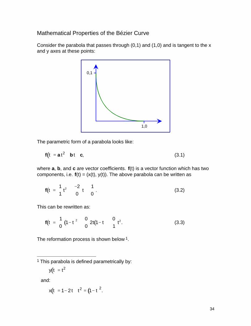
Consider the parabola that passes through (0,1) and (1,0) and is tangent to the xand y axes at these points:
1,0
0,1
The parametric form of a parabola looks like:
( )f a b ct t t= + +2 , (3.1)
where a, b, and c are vector coefficients. f(t) is a vector function which has twocomponents, i.e. f(t) = (x(t), y(t)). The above parabola can be written as
( )f t t t=
+−
+
11
20
10
2 . (3.2)
This can be rewritten as:
( ) ( ) ( )f t t t t t=
− +
− +
10
100
2 101
2 2. (3.3)
The reformation process is shown below 1.
1 This parabola is defined parametrically by:
( )y t t= 2
and:
( ) ( )x t t t t= − + = −1 2 12 2.
35
This is exactly the same curve as equation 3.2, so what advantage is there inrewriting? The advantage lies in the geometrical meaning of the coefficients:(1,0), (0,0), and (0,1). These are called control points. Together, the controlpoints form the control polygon.
Observe:
• The curve passes through the endpoints of the control polygon.
• The curve is cotangent to the control polygon at these endpoints.
The curve in this form is called the Bézier curve, and the observations hold ingeneral for any coefficients. This means that if the coefficients are changed, thecurve changes in an easy-to-understand way.
• The quadratic Bézier curve:
In vector form, it may be expressed as:
( ) ( )( ) ( ) ( )f t
x ty t
t t t t=
=
− +
− +
10
100
2 101
2 2.
36
The general form for a quadratic Bézier curve is:
( ) ( ) ( )f b b bt t t t t= − + − +02
1 221 2 1 . (3.4)
This is a parabola exactly as equation 3.1 but it is rewritten so that the controlpointsb0, b1, and b2 have geometrical significance as the control points of theparabola.
Bézier Curves of General Degree
The general form of a Bézier curve of degree n is:
( ) ( )f bt B ti in
i
n=
=∑
0
, (3.5)
where bi are vector coefficients, the now-familiar control points, and:
( ) ( )B tni
t tin i n i=
− −1 . (3.6)
( )ni
is the binomial coefficient; B t are called the Bernstein functions.i
n
37
Binomial Coefficients
The binomial coefficients, commonly derived from Pascal's triangle, may becomputed:
( )ni
n!i n i
=
−! !, (3.7)
for i, an integer ≥ 0.
Note that n0
= 1 and, in particular, 00
= 1.
Bernstein Functions
The Bernstein functions were originally devised by Bernstein to prove thefamous Weierstrass Theorem over 150 years ago. They are formally given by:
( ) ( ) ( )B tn
i n it ti
n n i i=−
− −!! !
.1 (3.8)
They have many useful properties for curve generation.
38
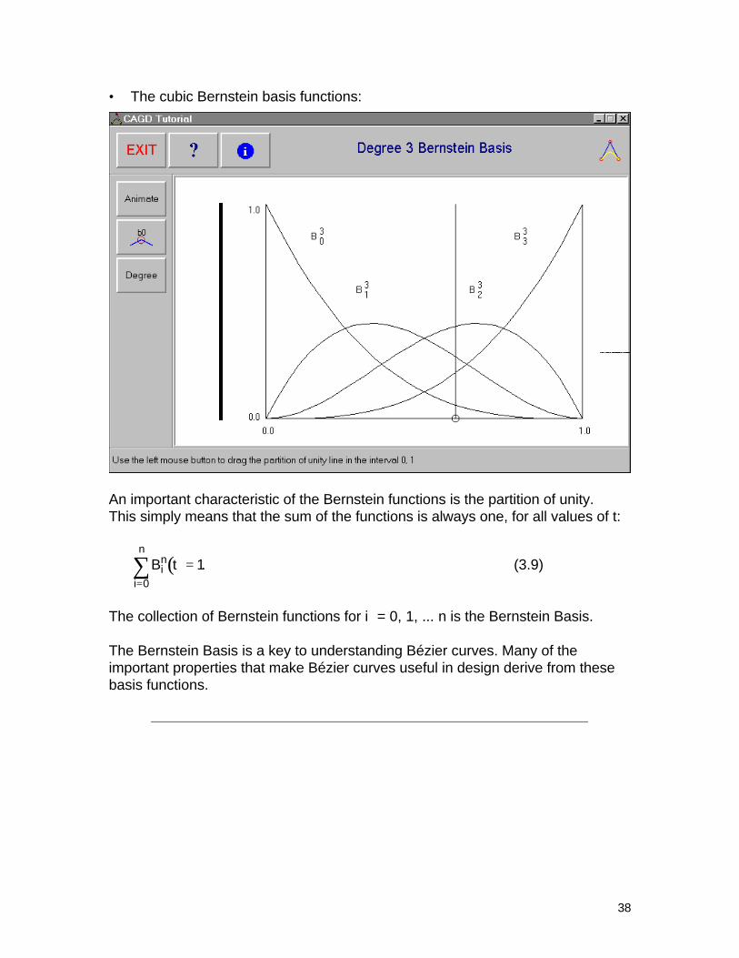
• The cubic Bernstein basis functions:
An important characteristic of the Bernstein functions is the partition of unity.This simply means that the sum of the functions is always one, for all values of t:
( )B tin
i
n
=∑ =
0
1. (3.9)
The collection of Bernstein functions for i = 0, 1, ... n is the Bernstein Basis.
The Bernstein Basis is a key to understanding Bézier curves. Many of theimportant properties that make Bézier curves useful in design derive from thesebasis functions.
39
Characteristics of the Bézier Curve
Bézier curves have a number of characteristics which define their behavior.
• Endpoint Interpolation
The Bézier curve interpolates the first and last points b0 and bn. In terms ofthe interpolation parameter t: f(0) = b0 and f(1) = bn. This property derivesfrom the Bernstein functions, since at the the endpoints the Bernsteinfunctions are zero except:
At B at B0 03
3 33b b, ; , .= =1 1
40
• Tangent Conditions
The Bézier curve is tangent to the first and last segments of the controlpolygon, at the first and last control points. In fact:
( ) ( ) ( ) ( )′ = − ′ = − −f b b f b b0 11 0 1n and nn n ,
where n is a constant.
41
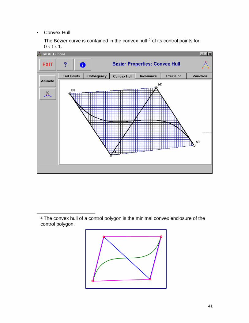
• Convex Hull
The Bézier curve is contained in the convex hull 2 of its control points for0 ≤ t ≤ 1.
2 The convex hull of a control polygon is the minimal convex enclosure of thecontrol polygon.
42
• Affine Invariance
The Bézier curve is affinely invariant with respect to its control points. Thismeans that any linear transformation (such as rotation or scaling) ortranslation of the control points defines a new curve which is just thetransformation or translation of the original curve.
43
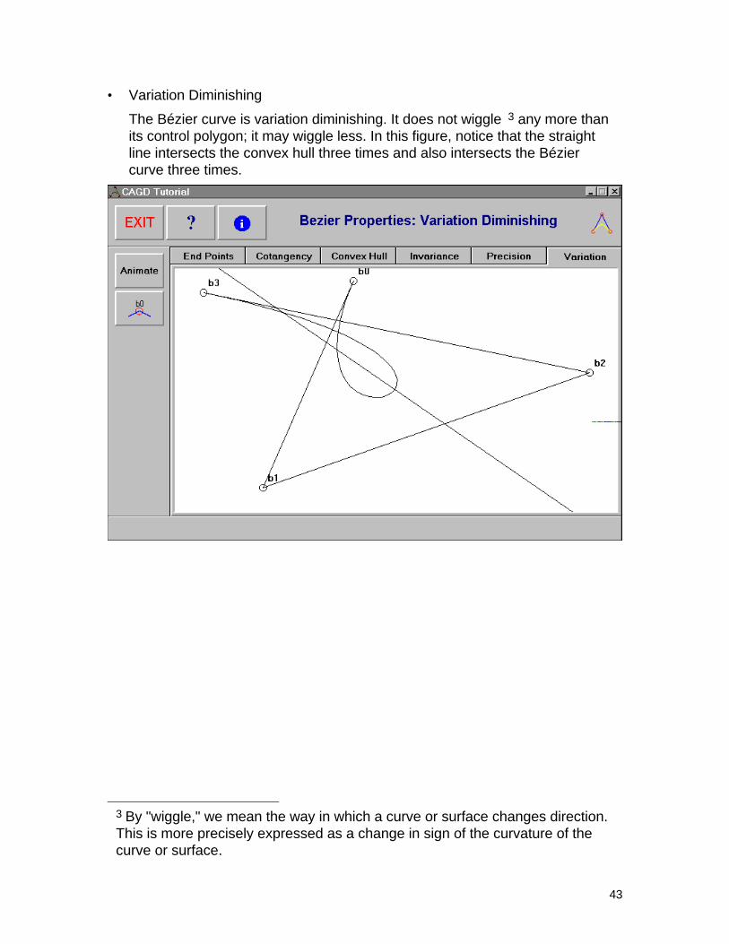
• Variation Diminishing
The Bézier curve is variation diminishing. It does not wiggle 3 any more thanits control polygon; it may wiggle less. In this figure, notice that the straightline intersects the convex hull three times and also intersects the Béziercurve three times.
3 By "wiggle," we mean the way in which a curve or surface changes direction.This is more precisely expressed as a change in sign of the curvature of thecurve or surface.
44
• Linear Precision
The Bézier curve has linear precision: If all the control points form a straightline, the curve also forms a line. This follows from the convex hull property;as the convex hull becomes a line, so does the curve.
45
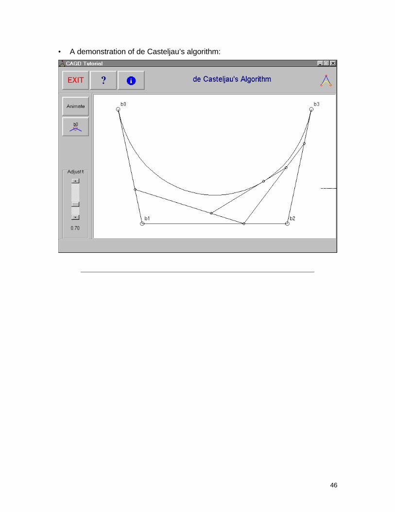
The de Casteljau Algorithm
Evaluation of the Bézier curve function at a given value t produces a point f(t).As t varies from 0 to 1, the point f(t) traces out the curve segment. One way toevaluate equation 3.5 is by direct substitution, that is, by applying the value of tto the formula and computing the result.
This is probably the worst method of evaluating a point on the curve! Numericalinstability, caused by raising small values to high powers, generates errors.
There are several better methods available for evaluating the Bézier curve. Onesuch method is the de Casteljau algorithm. This method not only provides ageneral, relatively fast, and robust algorithm, but it gives insight into the behaviorof Bézier curves and leads to several important operations on the curves, suchas:
• Computing Derivatives
The derivative of the curve gives the tangent vector at a point.
• Subdividing the Curve
It is sometimes necessary to take a single Bézier curve and produce twoseparate curve segments that together are identical to the original. Toaccomplish this, it is necessary to find two sets of control points for the twonew curves.
The de Casteljau algorithm can be regarded as repeated linear interpolation.
As described in the section on linear interpolation in Topic 2, PreliminaryMathematics, it is possible to interpolate between two points b0 and b1 with theequation:
( ) ( )f b bt t t= − +0 11 . (3.10)
If t = 0.5 then f(t) is the midpoint of the line between the endpoints.Equation 3.10 is just a Bézier curve of degree n = 1.
46
• A demonstration of de Casteljau’s algorithm:
47
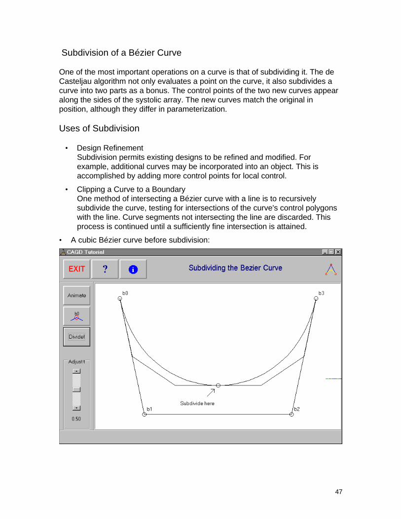
Subdivision of a Bézier Curve
One of the most important operations on a curve is that of subdividing it. The deCasteljau algorithm not only evaluates a point on the curve, it also subdivides acurve into two parts as a bonus. The control points of the two new curves appearalong the sides of the systolic array. The new curves match the original inposition, although they differ in parameterization.
Uses of Subdivision
• Design RefinementSubdivision permits existing designs to be refined and modified. Forexample, additional curves may be incorporated into an object. This isaccomplished by adding more control points for local control.
• Clipping a Curve to a BoundaryOne method of intersecting a Bézier curve with a line is to recursivelysubdivide the curve, testing for intersections of the curve's control polygonswith the line. Curve segments not intersecting the line are discarded. Thisprocess is continued until a sufficiently fine intersection is attained.
• A cubic Bézier curve before subdivision:
48
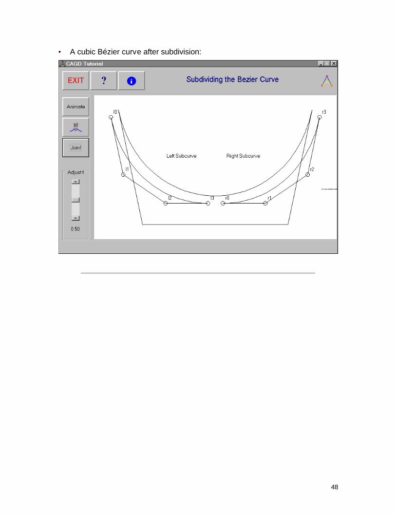
• A cubic Bézier curve after subdivision:
49
Higher Degree Bézier Curves
Bézier curves of any degree may be created. Degree 2 curves (quadraticcurves) are the lowest degree useful. Many commercial applications anddrawing packages use degree 3 Bézier curves (cubic curves) as a drawingprimitive.
• A degree 8 Bézier curve:
The Derivative of the Bézier Curve
It is a straightforward exercise in algebra to differentiate the Bézier function andthen to formulate the derivative in Bézier form. The derivative of a Bézier curveof degree n is:
( ) ( ) ( )′ = −+−
=
−
∑f b bt n B ti i in
i
n
11
0
1
. (3.12)
There is one less term in the derivative than in the original function. Also, thedegree of the Bernstein polynomials is one less. The control points for the
50
derivative curve are successive differences of the original curve's control points,having the form:
b bi i+ −1 .
Consider the derivatives at the endpoints of the Bézier curve:
( ) ( ) ( ) ( )′ = − ′ = − −f b b f b b0 11 0 1n n n n, , and (3.13)
where n is a constant.
The tangent endpoint property is derived from these two derivatives. It may beseen that the derivatives (the tangents) at the endpoints are n times the first andlast legs of the control polygon.
The hodograph of the Bézier curve is easy to construct in Bézier form. It is aBézier curve with control points given by:
∆b b bi i i n= − = −+1 01 1, , , , . i ... (3.14)
• The hodograph of the Bézier curve with its control polygon shown:
51
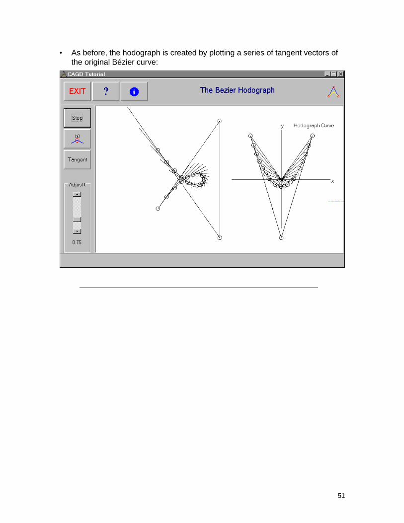
• As before, the hodograph is created by plotting a series of tangent vectors ofthe original Bézier curve:
52
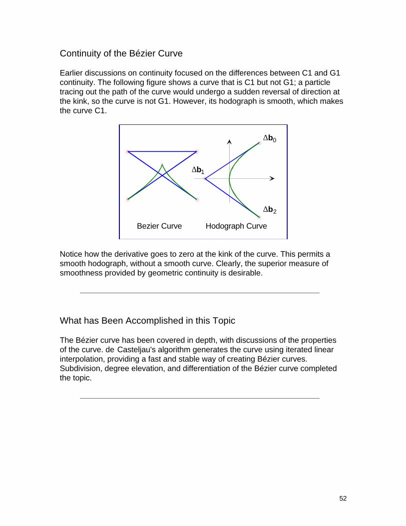
Continuity of the Bézier Curve
Earlier discussions on continuity focused on the differences between C1 and G1continuity. The following figure shows a curve that is C1 but not G1; a particletracing out the path of the curve would undergo a sudden reversal of direction atthe kink, so the curve is not G1. However, its hodograph is smooth, which makesthe curve C1.
Bezier Curve Hodograph Curve
∆b2
∆b1
∆b0
Notice how the derivative goes to zero at the kink of the curve. This permits asmooth hodograph, without a smooth curve. Clearly, the superior measure ofsmoothness provided by geometric continuity is desirable.
What has Been Accomplished in this Topic
The Bézier curve has been covered in depth, with discussions of the propertiesof the curve. de Casteljau's algorithm generates the curve using iterated linearinterpolation, providing a fast and stable way of creating Bézier curves.Subdivision, degree elevation, and differentiation of the Bézier curve completedthe topic.
53
Topic 4
Blossoms
54
Topic 4: Blossoms
In this topic, you will learn:
• What a blossom is, and the connection between blossoms and CAGD.
• The characteristics of blossoms.
• The application of blossoming to Bézier and B-spline curves.
• The uses of blossoms in CAGD.
Introduction
"What's in a name? That which we call a rose, by any other name wouldsmell as sweet."
Shakespeare, Romeo and Juliet.
In some instances, the name given to an object has little importance. Afragrance, for example, does not depend on its name. This is not true inmathematics, however; labels are significant. Well-chosen notation servesnot only as a tag, but also suggests how a concept is defined and used. Thisis especially true of a technique called blossoming. Its power lies in its abilityto suggest fundamentals, algorithms, and theorems in CAGD throughlabeling.
The theory of blossoms was introduced by Ramshaw and de Casteljau.
55
Blossom Basics
The basic principle of blossoming arises from linear interpolation 1. Recall thatb(0) and b(1) are points on the line segment at t = 0 and t = 1. Any point on theline is given by b(a). The distance from b(0) to b(a) is proportional to 0 - a .Similarly, the distance from b(a) to b(1) is proportional to 1 - a . It is veryuseful to think of a as a measure of how far a point travels from b(0) to b(a).For example, if a = 0.5, then b(a) is halfway between b(a) and b(1).
Notation
To further emphasize this relationship between a and b(0)-b(1), the functionalnotation is dropped and simply written b(0) = 0, b(1) = 1, and b(a) = a. a isspoken of loosely as the affine distance 2 from 0 to a.
Essentially, a point is designated by its parameter value a and the endpoints ofthe segment on which it lies, with the understanding that the point is obtainedby linear interpolation along the line.
This is shown in the following figure, which clarifies the new nomenclature.
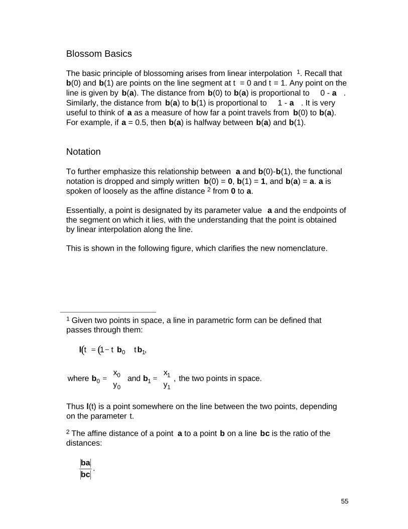
1 Given two points in space, a line in parametric form can be defined thatpasses through them:
( ) ( )l b bt t t= − +1 0 1,
where and the two points in space.0 1b b=
=
xy
xy
0
0
1
1,
Thus l(t) is a point somewhere on the line between the two points, dependingon the parameter t.
2 The affine distance of a point a to a point b on a line bc is the ratio of thedistances:
babc
.
56
l(0) l(1)l(a)
0 1a
is the same as:
Next an important extension is made to the notation in order to describe twolines that share a point. This is done by adding an additional digit as shown inthe figures below. First, add the digits to the two individual lines. The first lineis identified with a leading 0, it goes from 00 to 01. The second line has aleading 1, going from 10 to 11.
0 0
1 1
1 00 1
Next, bring the lines together so that they share an endpoint:
0 0
1 1
0 1 = 1 0
Note here (this is most important, even though it seems obvious) that point 01and point 10 are identical.
57
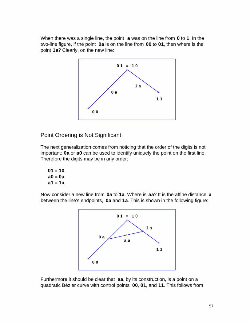
When there was a single line, the point a was on the line from 0 to 1. In thetwo-line figure, if the point 0a is on the line from 00 to 01, then where is thepoint 1a? Clearly, on the new line:
0 0
1 1
0 1 = 1 0
0 a1 a
Point Ordering is Not Significant
The next generalization comes from noticing that the order of the digits is notimportant: 0a or a0 can be used to identify uniquely the point on the first line.Therefore the digits may be in any order:
01 ≡ 10,a0 ≡ 0a,a1 ≡ 1a.
Now consider a new line from 0a to 1a. Where is aa? It is the affine distance abetween the line's endpoints, 0a and 1a. This is shown in the following figure:
0 0
1 1
0 1 = 1 0
0 a
1 a
a a
Furthermore it should be clear that aa, by its construction, is a point on aquadratic Bézier curve with control points 00, 01, and 11. This follows from
58
understanding de Casteljau's algorithm, which is base d on repeated linearinterpolation. The Bézier curve is shown in the following figure:
0 0
1 1
0 1 = 1 0
0 a
1 aa a
To add another control point, add another digit:
0 0 0 1 1 1
0 0 1 0 1 1
Here a convention is adopted of ordering the digits from smallest to largest.For example, 0a1 is preferred to 1a0, so long as 0 ≤ a ≤ 1. Sometimes commasare used to separate the digits, if required for clarity. The point 0,.5,1 is not0.5 1.
59
In the last figure, where is the point aaa? It can be found by recursivereplacement. This is the so-called blossoming principle 3. First find 00a, 0a1,and a11, on the appropriate lines. Then find 0aa and aa1. Finally, aaa may befound on the line between 0aa and aa1:
0 0 0 1 1 1
0 0 1 0 1 1
a 1 1
0 a 1
0 0 aa a a a a 10 a a
By construction, the point aaa is on the Bézier curve with control points 000,001, 011, and 111:
0 0 0 1 1 1
0 0 1 0 1 1
a 1 1
0 a 1
0 0 aa a a a a 10 a a
3 Informally, the digit that differs between two blossoms is replaced withanother value, giving the affine distance along the line segment for the newvalue.
Thus axx is found on the line segment between bxx and cxx, an affinedistance given by:
bxx axxcxx bxx
−−
.
60
Summary of Blossoming from Linear Interpolation
The generalization of this method for a Bézier curve of any degree should nowbe clear. The principles generated thus far may be summarized:
1. There is a Bézier curve of degree n that is given by points of the formaa....a. There are n a's.
2. The points are equivalent regardless of the ordering of the digits:a10 ≡ 01a ≡ 0a1.
3. The point 0...0a1...1 is an affine distance a along the line from 0...001...1 to0...011...1. In other words:
0a1 = (1 - a) 001 + (a) 011.
This is simple linear interpolation.
The History of Blossoms
It was proved by Ramshaw and de Casteljau that for every polynomial P(u) ofdegree n there is a unique function of n variables p(u 1, u2, ..., un) which has thethree properties listed in the summary above. Ramshaw called this function theblossom of the polynomial P(u). Quite often this blossom is given only as a listof its variables, as shown. The blossom notation suggests methods andalgorithms naturally. The de Casteljau algorithm arose by recursively applyingthe principles until a...a was found.
61
The Power of the Blossom Form
Blossoms are very powerful. Once the principle is understood, methods maybe generated to evaluate the Bézier curve, prove properties, define andevaluate B-spline curves, convert between B-spline and Bézier form, and muchmore.
The following section is intended for those who want more practice withblossoms. The material proves some new and some old things about Béziercurves by using blossoms. For example, one thing shown is that Bézier controlpoints always have the form:
bi = 0 01 1... ... (there are i ones).
The Bézier Curve in Blossom Form
Using the three properties of blossoms previously described, the following canbe observed:
( )For the blossom p u u uN1 2, ,..., :
( ) ( )( )( ) ( ) ( )( ) ( ) ( ) ( ) ( )
( ) ( ) ( ) ( )( ) ( ) ( )
p u u u p u u u u
u p u u up u u
u p u u u up u u u p u u
u p N u up
N u u p u p
N N
N N
, ,..., , ,...,
, ,..., , ,...,
, , ,..., , , ,..., , , ,...,
.
.
,..., ,..., , . . .
, ,..., ,..., .
= − ⋅ + ⋅
= − +
= − + − +
= − + − +
+ − +
−
−
1 0 1
1 0 1
1 0 0 2 1 01 11
1 0 0 1 0 01
1 01 1 1 1
2 2
1
1
The point p(u, u,..., u) is on the curve P(u) by the diagonal property. In the firstequation, the first u in the argument list is written as an affine combination:u = (1 - u).0 + u.1.
These steps are repeated for the next u in the argument list and the terms arecombined using the symmetry property to arrive at the third line. Continuing inthis manner, the argument list is exhausted.
62
The polynomial, as seen in the last line, is a summation of coefficients, writtenas blossoms, multiplied by the Bernstein basis polynomials. This polynomial isa Bézier curve of degree N. This can already be seen to be emerging in thethird equation; the polynomials in each term are quadratic Bernsteinpolynomials.
The coefficients, or control points, are blossoms evaluated with only 0's and1's, so the blossoms p(0, 0,..., 1, 1) are then the Bézier control points, that is:
( )bi p= 0 01 1,..., , ,..., ;
There are i ones in the blossom. This control point is the blossom evaluated at(N - i) 0's and i 1's; the order does not matter.
Evaluating a Blossom from Bézier Control Points
Suppose that a set of Bézier control points is given. What is the point given bythe blossom at u1...un? The blossom properties lead to an algorithm thatevaluates the blossom. It has the familiar form of iterated linear interpolation.
EvalBlossomProg: A General Blossom Algorithm
The de Casteljau algorithm generalizes to the EvalBlossom procedure. Thisassumes a [0, 1] range of curve parameterization, which may be a limitationin some circumstances. If EvalBlossom is extended to handle an arbitraryblossom parameterization, the result is the generalization known asEvalBlossomProg.
In this algorithm b[i] are the de Boor points, which will be discussed in depth inthe topic on The B-Spline Curve. t[i] are the blossom parameterization values.
What Has Been Accomplished in this Topic
A strong base of knowledge concerning the blossom form has been built. Thishas allowed the investigation of the Bézier curve more deeply, and willmotivate the development of B-spline curves.
64
Topic 5
The B-Spline Curve
65
Topic 5: The B-Spline Curve
In this topic, you will learn:
• The characteristics of B-spline curves.
• The derivation of B-spline curves from blossoming.
• The differences between Bézier and B-spline curve s.
Introduction
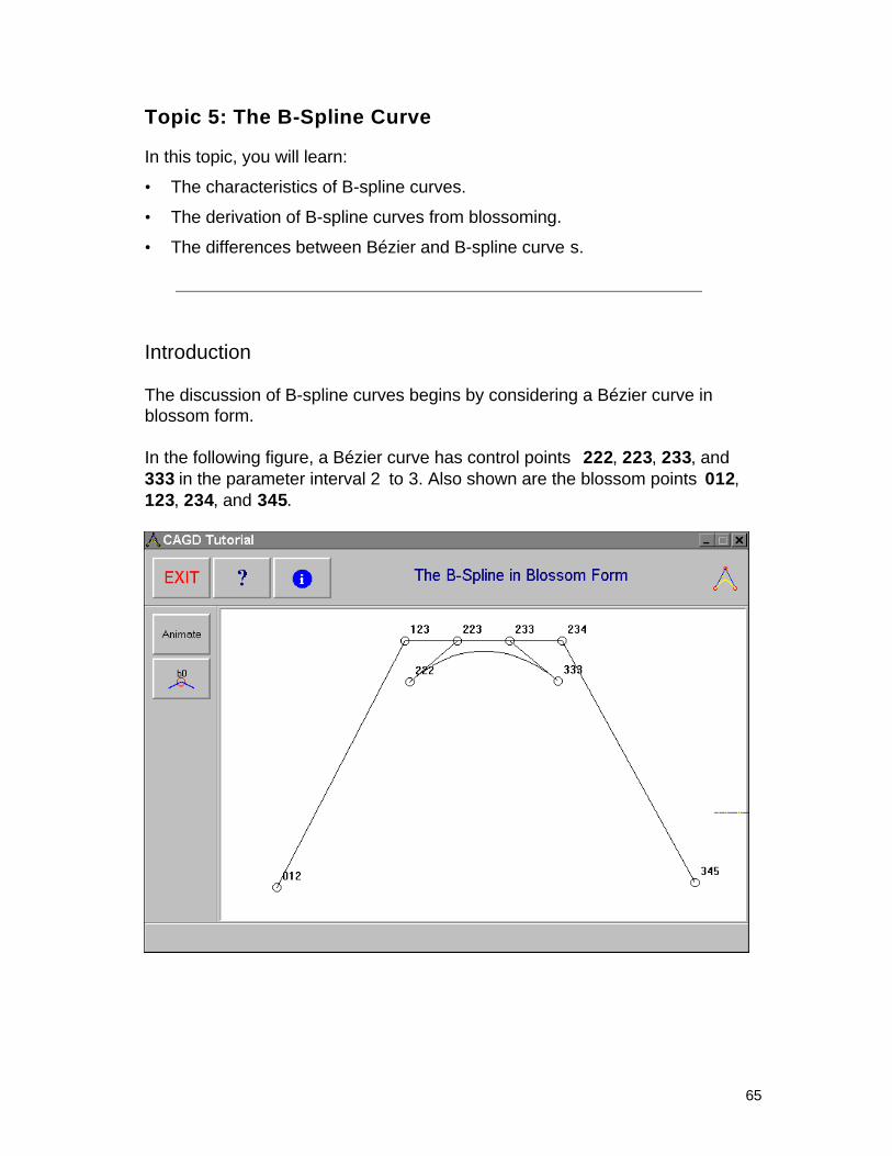
The discussion of B-spline curves begins by considering a Bézier curve inblossom form.
In the following figure, a Bézier curve has control points 222, 223, 233, and333 in the parameter interval 2 to 3. Also shown are the blossom points 012,123, 234, and 345.
66
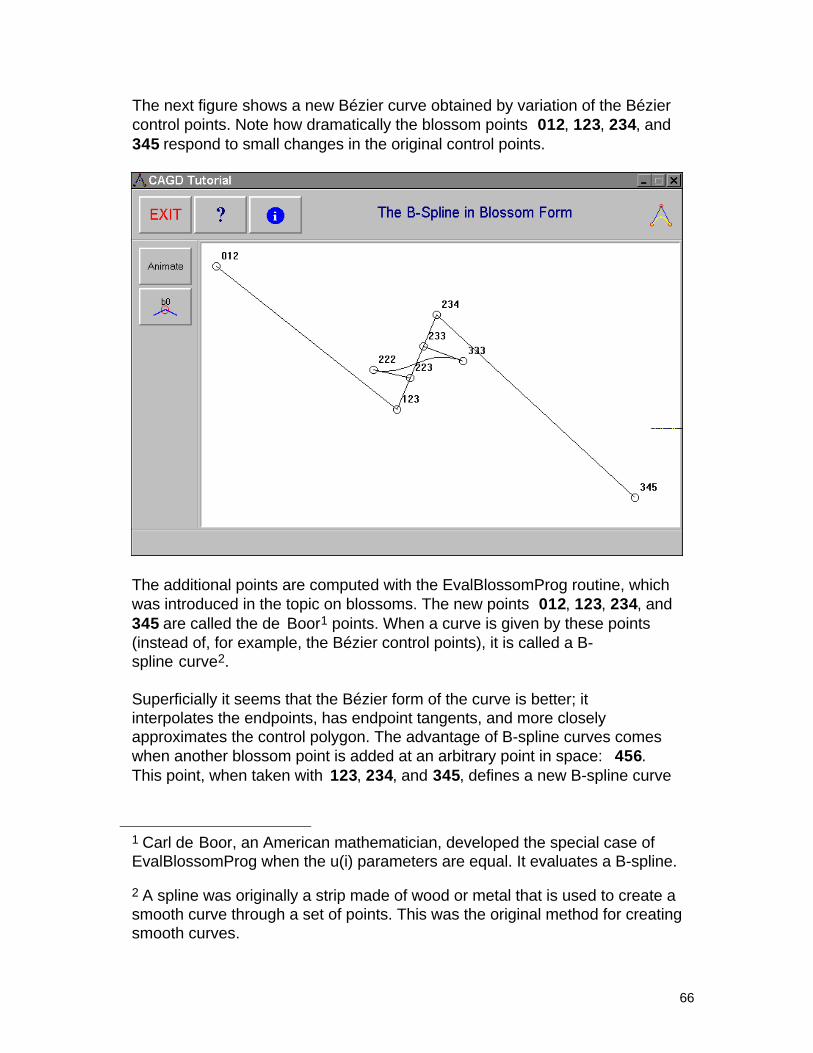
The next figure shows a new Bézier curve obtained by variation of the Béziercontrol points. Note how dramatically the blossom points 012, 123, 234, and345 respond to small changes in the original control points.
The additional points are computed with the EvalBlossomProg routine, whichwas introduced in the topic on blossoms. The new points 012, 123, 234, and345 are called the de Boor1 points. When a curve is given by these points(instead of, for example, the Bézier control points), it is called a B-spline curve2.
Superficially it seems that the Bézier form of the curve is better; itinterpolates the endpoints, has endpoint tangents, and more closelyapproximates the control polygon. The advantage of B-spline curves comeswhen another blossom point is added at an arbitrary point in space: 456.This point, when taken with 123, 234, and 345, defines a new B-spline curve
1 Carl de Boor, an American mathematician, developed the special case ofEvalBlossomProg when the u(i) parameters are equal. It evaluates a B-spline.
2 A spline was originally a strip made of wood or metal that is used to create asmooth curve through a set of points. This was the original method for creatingsmooth curves.
67
segment which runs from parameter value 3 to 4, as shown in the followingfigure:
68
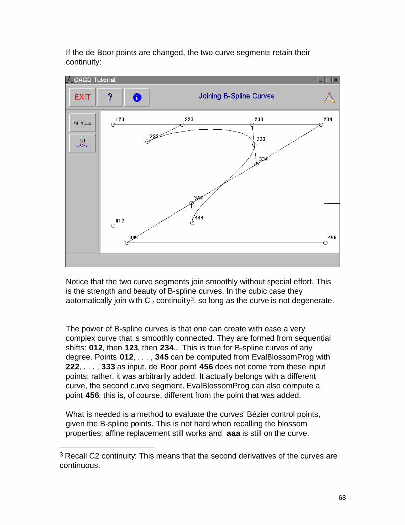
If the de Boor points are changed, the two curve segments retain theircontinuity:
Notice that the two curve segments join smoothly without special effort. Thisis the strength and beauty of B-spline curves. In the cubic case theyautomatically join with C 2 continuity3, so long as the curve is not degenerate.
The power of B-spline curves is that one can create with ease a verycomplex curve that is smoothly connected. They are formed from sequentialshifts: 012, then 123, then 234... This is true for B-spline curves of anydegree. Points 012, . . . , 345 can be computed from EvalBlossomProg with222, . . . , 333 as input. de Boor point 456 does not come from these inputpoints; rather, it was arbitrarily added. It actually belongs with a differentcurve, the second curve segment. EvalBlossomProg can also compute apoint 456; this is, of course, different from the point that was added.
What is needed is a method to evaluate the curves' Bézier control points,given the B-spline points. This is not hard when recalling the blossomproperties; affine replacement still works and aaa is still on the curve.
3 Recall C2 continuity: This means that the second derivatives of the curves arecontinuous.
69
These ideas may be used to derive the de Boor algorithm for evaluating B-splines.
The de Boor Algorithm
Start with the original set of de Boor points and find the point 2.5, 2.5, 2.5,which is in the curve between parameter values 2 and 3.
Here is the starting set of de Boor points:
Begin with the first leg of the curve ( 012 to 123). The digits 1 and 2 arecommon; 0 changes to 3 as we progress along the curve.
Where is 1, 2, 2.5 in this progression? It is linearly interpolated along theline; it is 2.5 / 3 in affine distance along the polygon leg:
Similarly, 2, 2.5, 3 is found on the second leg, and 2.5, 3, 4 on the last leg:
70
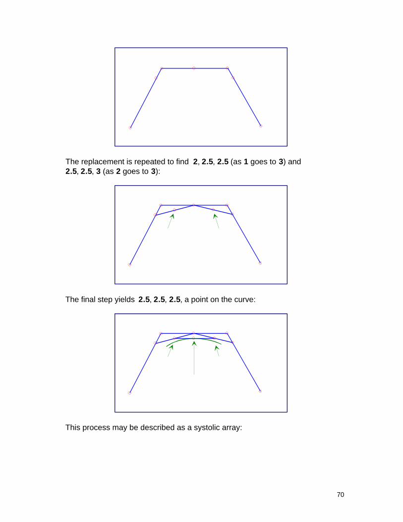
The replacement is repeated to find 2, 2.5, 2.5 (as 1 goes to 3) and2.5, 2.5, 3 (as 2 goes to 3):
The final step yields 2.5, 2.5, 2.5, a point on the curve:
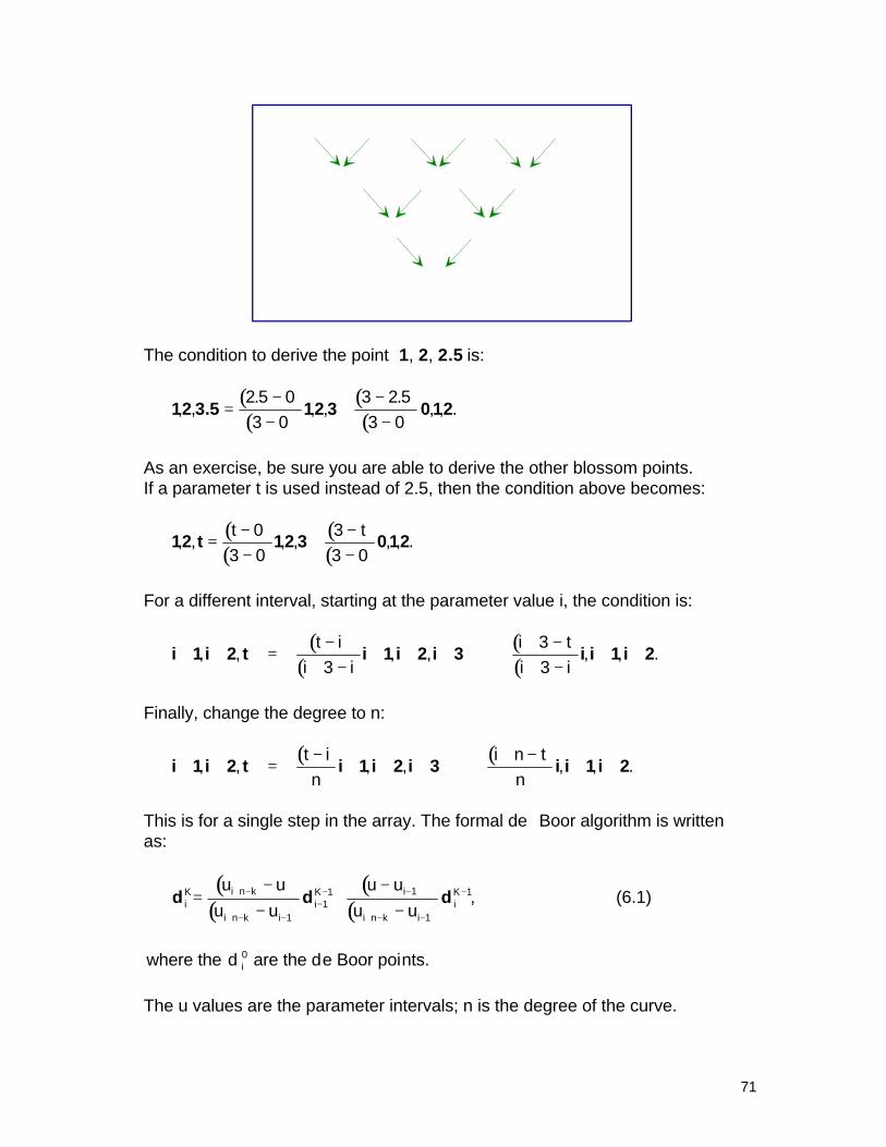
This process may be described as a systolic array:
71
The condition to derive the point 1, 2, 2.5 is:
( )( )
( )( )12 3.5 12 3 012, ,
., ,
.,=
−−
+−−
2 5 03 0
3 2 53 0
, .
As an exercise, be sure you are able to derive the other blossom points.If a parameter t is used instead of 2.5, then the condition above becomes:
( )( )
( )( )
12 t 12 3 012, , , , ,=−−
+−−
t t03 0
33 0
, .
For a different interval, starting at the parameter value i, the condition is:
( )( )
( )( )
i 1 i 2 t i 1 i 2 i 3 i i 1 i 2+ + =−
+ −+ + + +
+ −+ −
+ +, , , , ,t i
i ii ti i3
33
, .
Finally, change the degree to n:
( ) ( )i 1 i 2 t i 1 i 2 i 3 i i 1i 2+ + =
−+ + + +
+ −+ +, , , , ,
t in
i n tn
, .
This is for a single step in the array. The formal de Boor algorithm is writtenas:
( )( )
( )( )d d di
K i n k
i n k iiK i
i n k iiKu u
u uu u
u u=
−−
+−
−+ −
+ − −−
− −
+ − −
−
111 1
1
1, (6.1)
where the d are the de Boor points.i0
The u values are the parameter intervals; n is the degree of the curve.
72
This equation is the well-known de Boor algorithm. The de Boor points d areassociated with the blossom counterparts. The location of each succeedinglevel of points is made clear by the blossoms.
Summary of B-Splines in Blossom Form
The EvalBlossomProg procedure, in its more general form, gives:
• A method to evaluate B-spline curves.
• A reparameterization method for B-spline curves. This also permitssubdivision4 of the curve.
• A method to transform between B-spline curve segments and Béziercurves.
The B-spline control points in blossom form reveal much about the curvesegment:
• The number of digits equals the degree ( 012 is a control point for a cubiccurve).
• There are sequential shifts of adjacent digits (012, 123, 234...).
• The last digit of the first point and the first digit of the last point give thevalid parameterization interval for the curve segment. In the cubic example,this interval is in the range 2...3.
• Adding one new point to the existing set gives another segment of the B-spline curve. This new segment typically joins the existing curve withdegree n - 1 continuity.
4 Subdivision is the process, usually through reparameterization, of separating asingle curve segment into two parts.
73
Basis Functions
A single B-spline curve segment is defined much like a Bézier curve. It lookslike this:
( ) ( )d dt N tii
n
i==∑
0, (6.2)
where the d points are the de Boor points, the N(t) are the basis functions, andn is the degree of the curve.
The basis functions used here are different from the Bernstein basis functionsused by the Bézier curve.
Here are the cubic basis functions:
74
Here, the figure shows the cubic B-spline basis functions for a non-uniformknot sequence. The knot sequence is shown beneath the basis functions.
The basis functions for the B-spline curves are placed next to each other andoverlap in a similar way to the control points. When they are drawn togetherbell-shaped functions are generated that are zero outside a certain region of"support." It is also clear that they are simply translations of each other, foruniform knots.
It can be seen that (in the cubic case) for any parameter value t, only fourbasis functions are non-zero; thus only four control points affect the curve at t.If a control point is moved, it influences only a limited portion of the curve.
This locality of influence is known as the local support property. In the sameway as the Bernstein polynomials, the B-spline basis functions conform to thepartition of unity:
( )N ti∑ = 1.
This is used to prove that any point on the curve is a convex combination ofthe de Boor points, that is, it must be in the convex hull of the control pointsassociated with the non-zero basis functions.
75
What Has Been Accomplished in this Topic
The blossom principle has led naturally to B-splines, a type of curve usedextensively in industry. This topic discussed the relationship between B-splinesand Bézier curves, how the knot sequence modifies the curve, and how thecharacteristics of B-splines make them attractive as design tools.
76
Topic 6
Surfaces
77
Topic 6: Surfaces
In this topic, you will learn:
• The characteristics of surfaces.
• The use of Bézier surface patches.
• The use of B-spline surface patches.
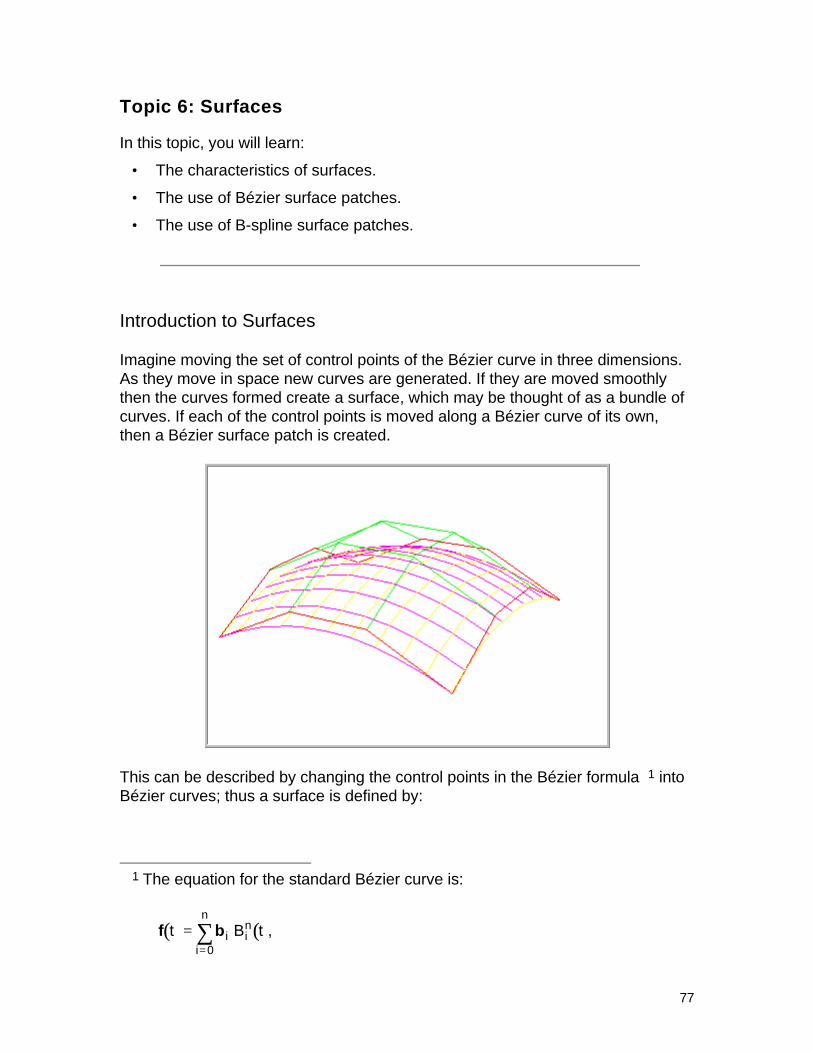
Introduction to Surfaces
Imagine moving the set of control points of the Bézier curve in three dimensions.As they move in space new curves are generated. If they are moved smoothlythen the curves formed create a surface, which may be thought of as a bundle ofcurves. If each of the control points is moved along a Bézier curve of its own,then a Bézier surface patch is created.
This can be described by changing the control points in the Bézier formula 1 intoBézier curves; thus a surface is defined by:
1 The equation for the standard Bézier curve is:
( ) ( )f bt B ti in
i
n=
=∑
0,
78
( ) ( ) ( )s bu v u B vi ii
n, .=
=∑
0(8.1)
Notice there is one parameter for the control curves and one for the "swept"curve. It is convenient to write the control curves as Bézier curves which havethe same degree as the original control curves. Given that:
• The ith control curve has control points ,ijb
then the surface given in equation 8.1 above can be written as:
( ) ( ) ( )s bu v B u B vij jj
m
ii
n, ,=
==∑∑
00(8.2)
where m is the degree of the control curves.
Such a surface can be thought of as nesting one set of curves inside another.From this simple characteristic, many properties and operations for surfaces maybe derived.
Simple algebra changes equation 8.2 above into:
( ) ( ) ( ) ( ) ( )s b bu v B u B v B v B uij jj
m
ii
n
ij i jj
m
i
n, .=
=
== ==∑∑ ∑∑
00 00(8.3)
That is, even though one curve was swept along the other, there is no preferreddirection. The surface patch could have been written as:
( ) ( ) ( )s bu v v B uj ji
n, =
=∑
0(8.4)
where:
( ) ( )b j ij ii
nv B v=
=∑b
0. (8.5)
The curve is simply swept in the other direction.
79
The set of control points forms a rectangular control mesh. A 3 by 3 (bicubic)control mesh is shown here:
There are 16 control points in the bicubic control mesh. In general there will be(n + 1) by (m + 1) control points. By convention, the "i" index is associated withthe "u" parameter, and the "j" index with the "v" parameter. Hence:
bi i n0 1, ... ,=
gives the Bézier curve:
( ) ( )b bu B ui in
i
n
, .0 00
==∑ (8.6)
80
Each marginal set of control points defines a Bézier curve (the four bordercurves) and each of these curves is a boundary of the Bézier surface patch.Such a curve is shown at the forward edge of the patch in the picture above.
81
Properties of the Bézier Surface Patch
Many of the properties of the Bézier surface are derived directly from those ofthe Bézier curve, especially those curves that form the boundaries of the patch:
• Endpoint Interpolation
The Bézier surface patch passes through all four corner control points.Formally, for the bicubic case:
( ) ( ) ( ) ( )b b b b b b b b0 0 01 10 1100 03 30 33, ; , ; , ; , .= = = =
• Tangent Conditions
The four border curves of the Bézier surface patch are cotangent to the firstand last segments of the each border control polygon, at the first and lastcontrol points. The normal to the surface patch at each vertex may be foundfrom the cross product of the tangents.
• Convex Hull
The Bézier surface patch is contained in the convex hull of its control meshfor 0 ≤ u ≤ 1 and 0 ≤ v ≤ 1.
• Affine Invariance
The Bézier surface patch is affinely invariant with respect to its controlmesh. This means that any linear transformation or translation of thecontrol mesh defines a new patch which is just the transformation ortranslation of the original patch.
• Variation Diminishing
Although this is difficult to define for surfaces, the control mesh suggeststhe shape of the patch.
• Planar Precision
The Bézier surface patch has planar precision: if all the points in the controlmesh lie in a plane, the surface patch will lie in the same plane; if all thepoints in the control mesh form a straight line, the surface is also reducedto a line.
82
Subdivision of the Bézier Surface Patch
As with the Bézier curve, the de Casteljau algorithm can be applied to subdividea Bézier surface patch. When a surface patch is subdivided, it yields foursubpatches that share a corner at the (u, v) subdivision point.
(u, v)
Recall that when a curve was subdivided, the new curve's control pointsappeared as the legs of a systolic array. In the surface case, subdividing eachrow of the control mesh produces points of the systolic array for each.
Each point on each leg of every row's systolic array now becomes a control pointfor a columnar set. A biquadratic case is shown here:
83
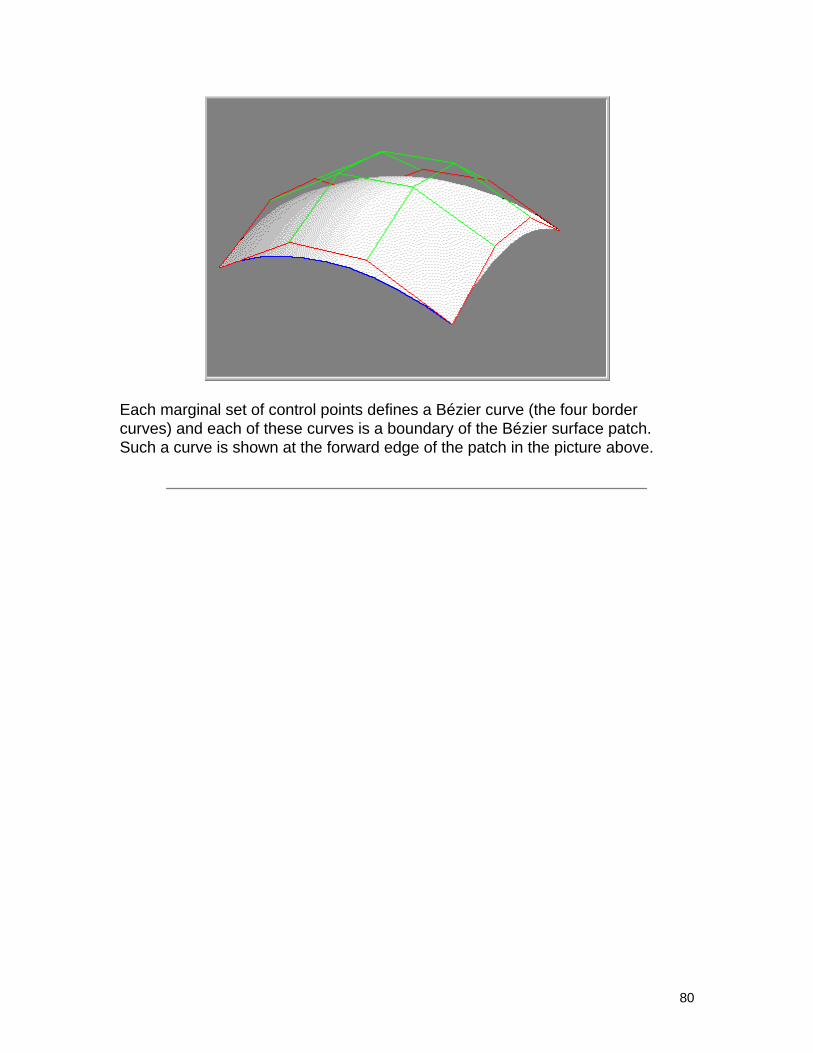
In this case, three points in each row produce five points after subdivision.
Now consider the points in columns, subdividing the columns with de Casteljau'salgorithm The points in the legs of their systolic arrays become the control pointsof the new subpatches. In the example above, rows with three control pointsproduce five "leg" points, that is, five columns of three points. Each column thenproduces five control points; so a 3 by 3 grid generates a 5 by 5 grid aftersubdivision:
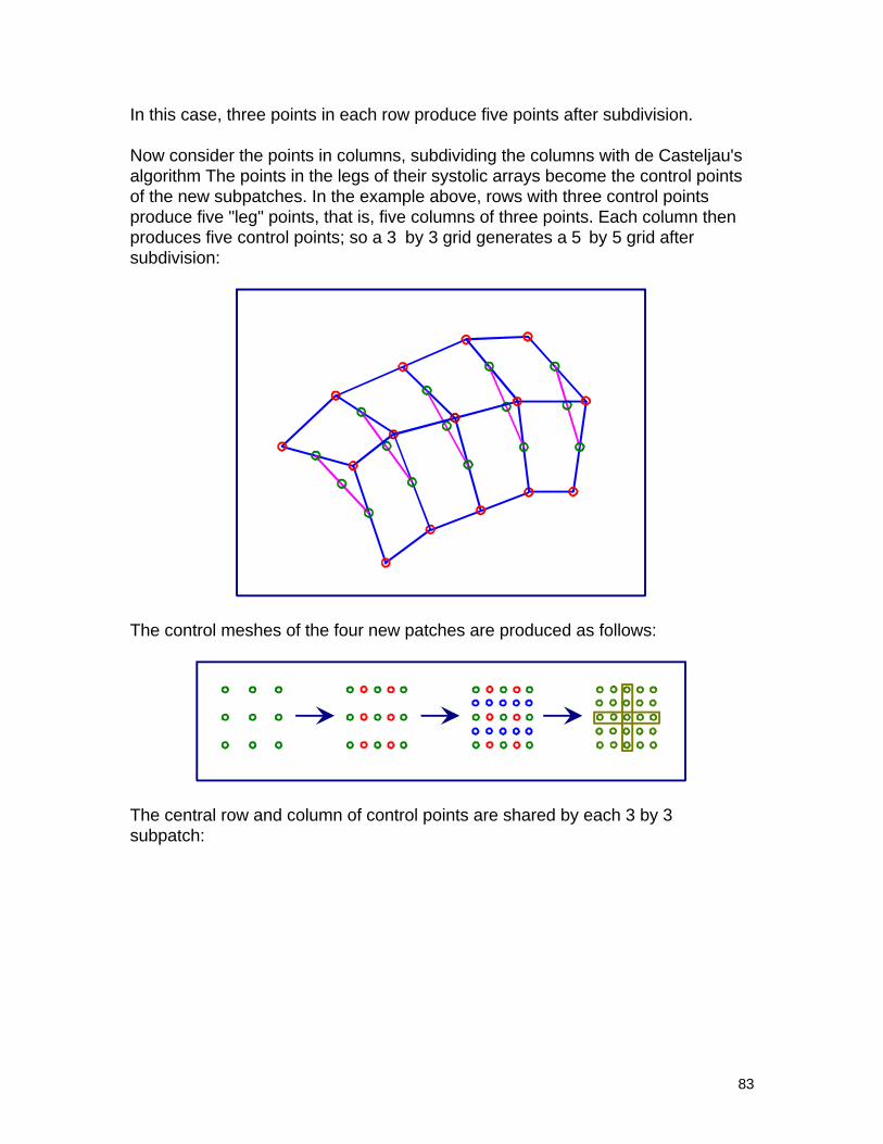
The control meshes of the four new patches are produced as follows:
The central row and column of control points are shared by each 3 by 3subpatch:
84
The order of the scheme does not matter. Columns may have been taken first,and then rows.
Subdivision is a basic operation of surfaces. Many "divide and conquer"algorithms are based on it. Imagine clipping a surface to a viewing window withthe two properties of:
• Convex hull property
• Subdivision
85
Uniform B-Spline Surfaces
As with the Bézier surface, the B-spline surface is defined as a nested bundle ofcurves, thus yielding:
( ) ( ) ( )s du v N u N vijj
M m
i
L n
i j, ,==
+ −
=
+ −
∑∑0
1
0
1
(8.7)
where:
• N are the familiar B - spline basis functions;i
• n, m are the degrees of the B-splines;
• L, M are the number of segments, so there are L by M patches.
All operations used for B-spline curves carry over to the surface via the nestingscheme, including knot insertion, de Boor's algorithm, and so on.
B-spline curves are especially convenient for obtaining continuity betweenpolynomial segments. This convenience is even stronger in the case of B-splinesurfaces:
• continuity is maintained between the subpatches.C Cm n− −1 1,
• B-splines define quilts of patches with corresponding design flexibility.
B-spline curves are more compact at representing a design than Bézier curves.This advantage is "squared" in the case of surfaces.
These advantages are tempered by the fact that operations are typically moreefficient on Bézier curves. Conventional wisdom says that it is best to designand represent surfaces as B-splines, and then convert to Bézier form foroperations.
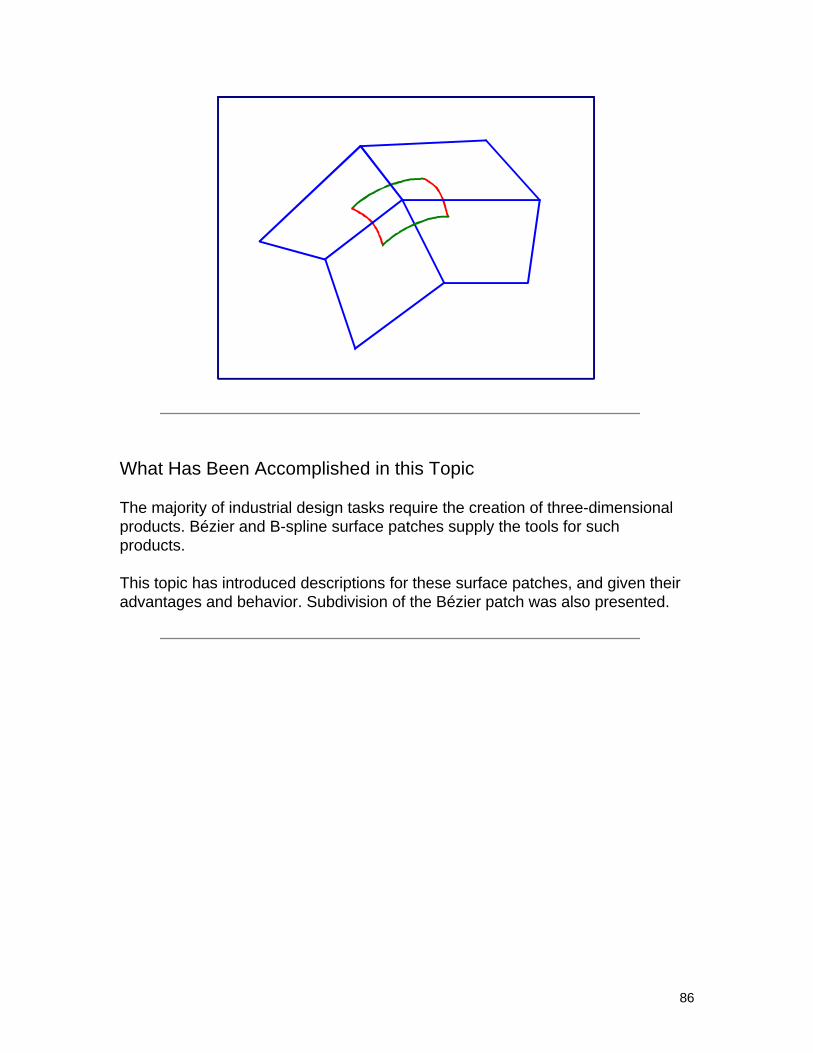
The following figure shows a simple B-spline surface patch:
86
What Has Been Accomplished in this Topic
The majority of industrial design tasks require the creation of three-dimensionalproducts. Bézier and B-spline surface patches supply the tools for suchproducts.
This topic has introduced descriptions for these surface patches, and given theiradvantages and behavior. Subdivision of the Bézier patch was also presented.
87
Bibliography
88
Bibliography
[Bajaj95] C. Bajaj and G. Xu, Modeling with cubic A patches, ACM Trans. onGraphics, 1995.
[Barnhill74] R. Barnhill. Smooth interpolation over triangles. In R. Barnhill and R.Riesenfeld, editors, Computer Aided Geometric Design, pages 45-70, AcademicPress, 1974.
[Barnhill82] R. Barnhill. Coons patches. Computers in Industry, 3: 37-43, 1982.
[Barnhill74] R. Barnhill and R. F. Riesenfeld, editors. Computer Aided GeometricDesign. Academic Press, 1974. This contains the proceedings of the firstconference on CAGD.
[Barsky81] B. Barsky. The Beta-spline: A Local Representation Based on ShapeParameters and Fundamental Geometric Measures. Ph.D. thesis, Dept. ofComputer Science, University of Utah, 1981.
[Bartels87] R. Bartels, J. Beatty, and B. Barsky, An Introduction of Splines forUse in Computer Graphics and Geometric Modeling. Morgan Kaufmann, 1987.
[Blinn78] Simulation of wrinkled surfaces. Computer Graphics, 12(3): 286-292.
[Bloor91] M. Bloor and M. Wilson, Generating blending surfaces with partialdifferential equations, CAD 25 (1991) pp. 251-256.
[Boehm83] W. Boehm and G. Farin. Concerning subdivision of Bézier triangles.Computer Aided Design, 15(5): 260-261, 1983. Letter to the editor.
[Boehm84] W. Boehm, G. Farin, and J. Kahmann. A survey of curve and surfacemethods in CAGD. Computer Aided Geometric Design, 1(1): 1-60, 1984.
[Catmull78] E. Catmull and J. Clark. Recursively generated B-spline surfaces onarbitrary topological meshes. Computer Aided Design, 10(6):350-355, 1978.
[Catmull & Rom74] E. Catmull and R. Rom. A class of local interpolating splines.In R. Barnhilll and R. Riesenfeld, editors, Computer Aided Geometric Design,pages 317-326, Academic Press, 1974.
[Catmull74] E. Catmull. A Subdivision Algorithm for the Computer Display ofCurved Surfaces, Ph.D. thesis, Dept. of Computer Science, University of Utah,1974.
89
[Charrot84] P. Charrot and J. Gregory. A pentagonal surface patch for computeraided geometric design. Computer Aided Geometric Design, 1(1): 87-94, 1984.
[Chandru89] V. Chandru, D. Dutta, and C. M. Hoffmann. On the geometry ofdupin cyclides. The Visual Computer, 5(5): 277-290, 1989.
[Chiyokura83] H. Chiyokura and F. Kimura. Design of solids with free-formsurfaces. Computer Graphics, 17(3): 289-298, 1983.
[Chiyokura86] H. Chiyokura. Solid Modeling with Designbase, Theory andimplementation, Addison Wesley, New York, 1986.
[Coons64] S. Coons. Surfaces for computer aided design. Technical Report,MIT, 1964. Available as AD 663 504 from the National Technical InformationService, Springfield, VA 22161. This is the first of Coons' papers on his patch.
[Dahman89] W. Dahman. Smooth Piecewise Quadric Shapes. Math. Methods inCAGD. T. Lyche, L. Schumaker, editors, Academic Press, Boston, 1989.
[deBoor78] C. de Boor. A Practical Guide to Splines. Springer, 1978. This is theclassical reference to splines written for the numerical analyst.
[Doo78] D. Doo and M. Sabin. Behavior of recursive division surfaces nearextraordinary points. Computer Aided Design, 10(6): 356-360, 1978.
[Farin93] G. Farin. Curves and Surfaces for Computer Aided Geometric Design.Third Edition. Academic Press, 1993. This is the popular work specifically onparametric curves and surfaces.
[Faux79] I. Faux and M. Pratt. Computational Geometry for Design andManufacture. Ellis Horwood, 1979. This is the first text on the subject, still aninteresting read.
[Filip86] D. Filip. Adaptive subdivision algorithms for a set of Bézier triangles.Computer Aided Design, 18(2): 74-78, 1986.
[Foley92] J. Foley and A. Van Dam. Fundamentals of Interactive ComputerGraphics. Addison-Wesley, 1992. A popular text book on computer graphics,this text has a few introductory chapters on CAGD.
90
[Forrest72] A. Forrest. On Coons' and other methods for the representation ofcurved surfaces. Computer Graphics and Image Processing, 1(4): 341-359,1972.
[Goldman88] R. Goldman, Urn Models, Approximations and Splines. Journal ofApproximation Theory, 54: 1-66, 1988.
[Goldman85] R. Goldman. The method of resolvents: a technique for theimplicitization, inversion, and intersection of non-planar, parametric, rationalcubic curves. Computer Aided Geometric Design, 2(4): 237-255,1985.
[Goshtasby93] A. Goshtasby. Design and recovery of 2D and 3D shapes usingrational Gaussian curves and surfaces. Int. J. of Computer Vision, 10(3): 233-256, 1993.
[Gregory80] J. Gregory and P. Charrot. A C 1 triangular interpolation patch forcomputer-aided geometric design. Computer Graphics and Image Processing,13(1): 80-87, 1980.
[Hoffman89] C. Hoffmann. Geometric & Solid Modeling. Morgan Kaufmann,1989.
[Hosaka84] M. Hosaka and F. Kimura. Non-four-sided patch expressions withcontrol points. Computer Aided Geometric Design, 1(1): 75-86, 1984.
[Hoschek89] J. Hoschek and K. Lasser. Grundlagen der GeometrischenDatenverarbeiturng. B.G. Teubner, Stuttgart, 1989. English translation:Fundamentals of Computer Aided Geometric Design, Jones and Bartlett,publishers. This is a text that is very broad and comprehensive.
[Loop90] C. Loop and T. DeRose. Generalized B-spline surfaces of arbitrarytopology. Computer Graphics, 24(4): 347-356, 1990.
[Nasri91] A. Nasri. Boundary-corner control in recursive-subdivision surfaces.Computer Aided Design, 23(6): 405-410, 1991.
[Nielson79] G. Nielson. The side-vertex method for interpolation in triangles.Journal of Approximation Theory, 25: 318-336, 1979.
[Nielson86] G. Nielson. A rectangular nu-spline for interactive surface design.IEEE Computer Graphics and Applications, 6(2): 35-41. 1986.
[Nielson87] G. Nielson. A transfinite, visually continuous, triangular interpolant.In G. Farin, editor, Geometric Modeling: Algorithms and New Trends, pages 235-246, SIAM, Philadelphia, 1987.
91
[Pavlidis83] T. Pavlidis. Curve fitting with conic splines. ACM Transactions onGraphics, 2(1): 1-31, 1983.
[Plowman95] D. Plowman and P. Charrot. A practical implementation of vertexblend surfaces using an n-sided patch. The Mathematics of Surfaces, VI, G.Mullineux, editor, Oxford University Press, 1995.
[Powell77] M. Powell and M. Sabin. Piecewise quadratic approximations ontriangles. ACM Transactions on Mathematical Software, 3: 316-325, 1977.
[Pratt90] M. Pratt. Cyclides in computer aided geometric design. Computer AidedGeometric Design, 7(1-4): 221-242, 1990.
[Rockwood89] A. Rockwood. The displacement method for implicit blendingsurfaces in solid models. ACM TOGS, 8(4): 279-297, Oct. 1989.
[Sabin76] M. Sabin. The use of piecewise forms for the numerical representationof shape. Ph.D. thesis, Hungarian Academy of Sciences, Budapest, Hungary,1976.
[Sabin86] M. Sabin. Some negative results in n-sided patches. Computer AidedDesign, 18(1): 38-44, 1986.
[Salmon1885] G. Salmon. Modern Higher Algebra. Chelsea, New York, 5thedition, pp. 83-86, 1885. An excellent Victorian text on geometry. Be careful howyou name books-notice the date!
[Sarraga90] R. F. Sarraga. Computer modeling of surfaces with arbitraryShapes. IEEE Computer Graphics and Applications (1990), 67-77.
[Sederberg83] T. Sederberg. Implicit and parametric curves and surfaces forcomputer aided geometric design. Ph.D. thesis, Purdue University, 1983.
[Sederberg95] T. Sederberg. Implicitization using moving curves and surfaces.Proc. of ACM SIGGRAPH ‘95, August 1995.
[Sederberg85] T. Sederberg. Piecewise algebraic surface patches. CAGD 2,1985.
[Varady87] T. Varady. Survey and new results in n-sided patch generation. inR. Martin, editor, The Mathematics of Surfaces II, pages 203-236, OxfordUniversity Press, 1987.
92
[Varady91] T. Varady. Overlap patches: a new scheme for interpolating curvenetworks with n-sided regions. CAGD 8 (1991), 7-27.
[Varady95] T. Varady and A. Rockwood. Vertex blending based on the setbacksplit. Math. Methods in CAGD III, M. Daehlen et al, editors, Vanderbilt UniversityPress, 1995.
[Zhao94] Y. Zhao and A. Rockwood. A convolution approach to N-sided patchesand vertex blending, designing fair curves and surfaces. N. Sapidis, editor,SIAM, Philadelphia, 1994.