76
INTRODUCTION TO DATA SCIENCE JOHN P DICKERSON PREM SAGGAR Lecture #5 – 9/12/2018 CMSC320 Mondays and Wednesdays 2pm – 3:15pm

INTRODUCTION TO DATA SCIENCEJOHN P DICKERSON
PREM SAGGAR
Lecture #5 – 9/12/2018
CMSC320Mondays and Wednesdays 2pm – 3:15pm

ANNOUNCEMENTSProject 1 out by the end of the week
Please, go find a job! Career fair in the Xfinity Center!
2

AN EXAMPLE OF BIASED SAMPLING
3

REVIEW OF LAST CLASSShift thinking from:
Imperative code to manipulate data structures
to: Sequences/pipelines of operations on data
Two key questions:1. Data Representation, i.e., what is the natural way to think
about given data
2. Data Processing Operations, which take one or more datasets as input and produce
4

REVIEW OF LAST CLASS1. NumPy: Python Library for Manipulating nD Arrays• A powerful n-dimensional array object.
• Homogeneous arrays of fixed size
• Operations like: indexing, slicing, map, applying filters
• Also: Linear Algebra, Vector operations, etc.
• Many other libraries build on top of NumPy
5
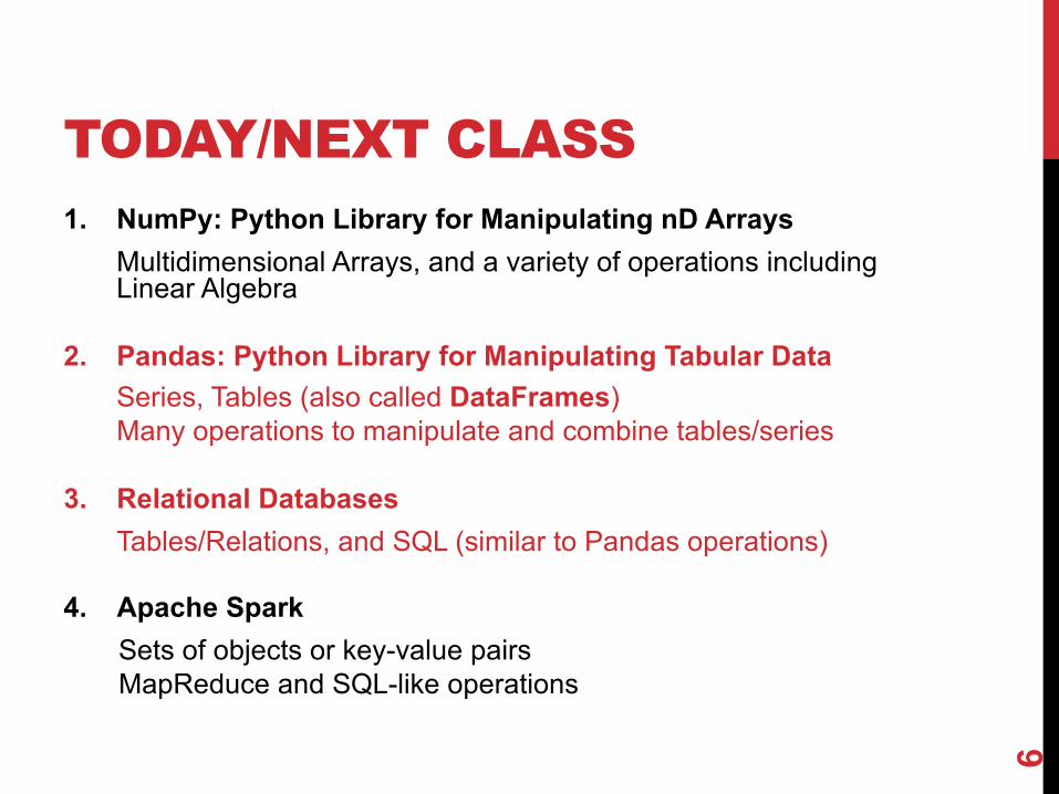
TODAY/NEXT CLASS1. NumPy: Python Library for Manipulating nD Arrays
Multidimensional Arrays, and a variety of operations including Linear Algebra
2. Pandas: Python Library for Manipulating Tabular Data Series, Tables (also called DataFrames)Many operations to manipulate and combine tables/series
3. Relational DatabasesTables/Relations, and SQL (similar to Pandas operations)
4. Apache SparkSets of objects or key-value pairs MapReduce and SQL-like operations
6

TODAY’S LECTURE
7
Data collection
Data processing
Exploratory analysis
&Data viz
Analysis, hypothesis testing, &
ML
Insight & Policy
Decision

TODAY/NEXT CLASS§ Tables
§ Abstraction§ Operations
§ Pandas
§ Tidy Data
§ SQL
8

TABLES
9
ID age wgt_kg hgt_cm
1 12.2 42.3 145.1
2 11.0 40.8 143.8
3 15.6 65.3 165.3
4 35.1 84.2 185.8
Observations,Rows, or
Tuples
Variables(also called Attributes, or
Columns, or Labels)
Special Column, called “Index”, or “ID”, or “Key”
Usually, no duplicates Allowed

TABLES
10
ID age wgt_kg hgt_cm
1 12.2 42.3 145.1
2 11.0 40.8 143.8
3 15.6 65.3 165.3
4 35.1 84.2 185.8
ID Address1 College Park, MD, 20742
2 Washington, DC, 20001
3 Silver Spring, MD 20901
199.72.81.55 - - [01/Jul/1995:00:00:01 -0400] "GET /history/apollo/ HTTP/1.0" 200 6245
unicomp6.unicomp.net - - [01/Jul/1995:00:00:06 -0400] "GET /shuttle/countdown/ HTTP/1.0" 200 3985
199.120.110.21 - - [01/Jul/1995:00:00:09 -0400] "GET /shuttle/missions/sts-73/mission-sts-73.html HTTP/1.0" 200 4085

1. SELECT/SLICINGSelect only some of the rows, or some of the columns, or a combination
11
ID age wgt_kg hgt_cm1 12.2 42.3 145.12 11.0 40.8 143.83 15.6 65.3 165.34 35.1 84.2 185.8
ID age1 12.22 11.03 15.64 35.1
Only columnsID and Age
Only rows with wgt > 41
Both
ID age wgt_kg hgt_cm1 12.2 42.3 145.13 15.6 65.3 165.34 35.1 84.2 185.8
ID age
1 12.2
3 15.6
4 35.1

2. AGGREGATE/REDUCECombine values across a column into a single value
12
ID age wgt_kg hgt_cm1 12.2 42.3 145.1
2 11.0 40.8 143.8
3 15.6 65.3 165.3
4 35.1 84.2 185.8
SUM
SUM(wgt_kg^2 - hgt_cm)
73.9 232.6 640.0
MAX 35.1 84.2 185.8
14167.66What about ID/Index column?Usually not meaningful to aggregate across itMay need to explicitly add an ID column

3. MAPApply a function to every row, possibly creating more or fewer columns
13
ID Address1 College Park, MD, 207422 Washington, DC, 200013 Silver Spring, MD 20901
Variations that allow one row to generate multiple rows in the output (sometimes called “flatmap”)
ID City State Zipcode1 College
ParkMD 20742
2 Washington DC 200013 Silver
SpringMD 20901

4. GROUP BYGroup tuples together by column/dimension
14
ID A B C1 foo 3 6.62 bar 2 4.73 foo 4 3.14 foo 3 8.05 bar 1 1.26 bar 2 2.57 foo 4 2.38 foo 3 8.0
ID B C1 3 6.63 4 3.14 3 8.07 4 2.38 3 8.0
ID B C2 2 4.75 1 1.26 2 2.5
A = foo
A = barBy ‘A’

4. GROUP BYGroup tuples together by column/dimension
15
ID A B C1 foo 3 6.62 bar 2 4.73 foo 4 3.14 foo 3 8.05 bar 1 1.26 bar 2 2.57 foo 4 2.38 foo 3 8.0
By ‘B’
ID A C5 bar 1.2
B = 1
ID A C2 bar 4.76 bar 2.5
ID A C3 foo 3.17 foo 2.3
ID A C1 foo 6.64 foo 8.08 foo 8.0
B = 3
B = 2
B = 4
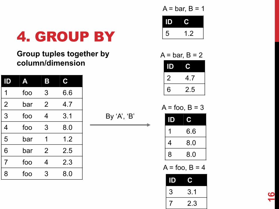
4. GROUP BYGroup tuples together by column/dimension
16
ID A B C1 foo 3 6.62 bar 2 4.73 foo 4 3.14 foo 3 8.05 bar 1 1.26 bar 2 2.57 foo 4 2.38 foo 3 8.0
By ‘A’, ‘B’
ID C5 1.2
A = bar, B = 1
ID C2 4.76 2.5
ID C3 3.17 2.3
ID C1 6.64 8.08 8.0
A = foo, B = 3
A = bar, B = 2
A = foo, B = 4

5. GROUP BY AGGREGATECompute one aggregatePer group
17
ID A B C1 foo 3 6.62 bar 2 4.73 foo 4 3.14 foo 3 8.05 bar 1 1.26 bar 2 2.57 foo 4 2.38 foo 3 8.0
Group by ‘B’Sum on C
17
ID A C5 bar 1.2
B = 1
ID A C2 bar 4.76 bar 2.5
ID A C3 foo 3.17 foo 2.3
ID A C1 foo 6.64 foo 8.08 foo 8.0
B = 3
B = 2
B = 4
Sum (C)1.2
B = 1
B = 3
B = 2
B = 4
Sum (C)22.6
Sum (C)7.2
Sum (C)5.4
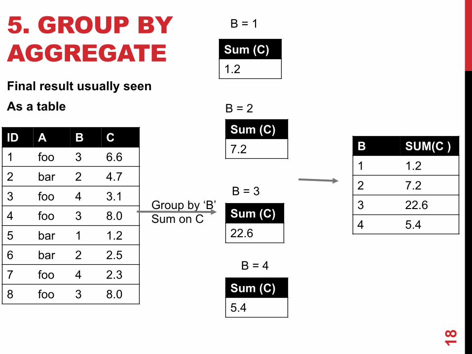
5. GROUP BY AGGREGATEFinal result usually seenAs a table
ID A B C1 foo 3 6.62 bar 2 4.73 foo 4 3.14 foo 3 8.05 bar 1 1.26 bar 2 2.57 foo 4 2.38 foo 3 8.0
Group by ‘B’Sum on C
18
Sum (C)1.2
B = 1
B = 3
B = 2
B = 4
Sum (C)22.6
Sum (C)7.2
Sum (C)5.4
B SUM(C )1 1.22 7.23 22.64 5.4

6. UNION/INTERSECTION/DIFFERENCESet operations – only if the two tables have identical attributes/columns
19
ID A B C1 foo 3 6.62 bar 2 4.73 foo 4 3.14 foo 3 8.0
19
ID A B C5 bar 1 1.26 bar 2 2.57 foo 4 2.38 foo 3 8.0
U
ID A B C1 foo 3 6.62 bar 2 4.73 foo 4 3.14 foo 3 8.05 bar 1 1.26 bar 2 2.57 foo 4 2.38 foo 3 8.0Similarly Intersection and Set Difference
manipulate tables as Sets
IDs may be treated in different ways, resulting in somewhat different behaviors
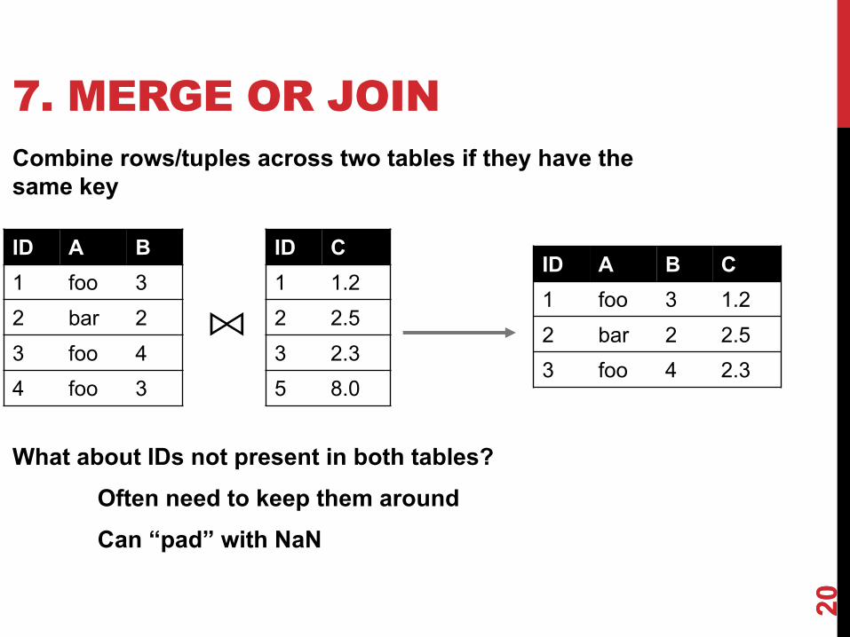
7. MERGE OR JOINCombine rows/tuples across two tables if they have the same key
20
ID A B1 foo 32 bar 23 foo 44 foo 3
20
ID C1 1.22 2.53 2.35 8.0
ID A B C1 foo 3 1.22 bar 2 2.53 foo 4 2.3
⨝
What about IDs not present in both tables?Often need to keep them aroundCan “pad” with NaN

7. MERGE OR JOINCombine rows/tuples across two tables if they have the same keyOuter joins can be used to ”pad” IDs that don’t appear in both tables
Three variants: LEFT, RIGHT, FULLSQL Terminology -- Pandas has these operations as well
21
ID A B1 foo 32 bar 23 foo 44 foo 3
21
ID C1 1.22 2.53 2.35 8.0
ID A B C1 foo 3 1.22 bar 2 2.53 foo 4 2.34 foo 3 NaN5 NaN NaN 8.0
⟗

SUMMARY§ Tables: A simple, common abstraction
§ Subsumes a set of “strings” – a common input
§ Operations§ Select, Map, Aggregate, Reduce, Join/Merge,
Union/Concat, Group By
§ In a given system/language, the operations may be named differently§ E.g., SQL uses “join”, whereas Pandas uses “merge”
§ Subtle variations in the definitions, especially for more complex operations
22

How many tuples in the answer?
A. 1B. 3C. 5D. 8
ID A B C1 foo 3 6.62 baz 2 4.73 foo 4 3.14 baz 3 8.05 bar 1 1.26 bar 2 2.57 foo 4 2.38 foo 3 8.0
Group By ‘A’

How many groups in the answer?
A. 1B. 3C. 4D. 6
ID A B C1 foo 3 6.62 baz 2 4.73 foo 4 3.14 baz 3 8.05 bar 1 1.26 bar 2 2.57 foo 4 2.38 foo 3 8.0
Group By ‘A’, ‘B’

How many tuples in the answer?
A. 1B. 2C. 4D. 6
ID A B1 foo 32 bar 24 foo 45 foo 3
ID C2 1.24 2.56 2.37 8.0
⨝

How many tuples in the answer?
A. 1B. 4C. 6D. 8
ID A B1 foo 3
2 bar 2
4 foo 4
5 foo 3
ID C2 1.2
4 2.5
6 2.3
7 8.0
⟗
FULL OUTER JOIN
All IDs will be present in the answerWith NaNs

TODAY/NEXT CLASS§ Tables
§ Abstraction§ Operations
§ Pandas
§ Tidy Data
§ SQL and Relational Databases
27

PANDAS: HISTORY§ Written by: Wes McKinney
§ Started in 2008 to get a high-performance, flexible tool to
perform quantitative analysis on financial data
§ Highly optimized for performance, with critical code paths written in Cython or C
§ Key constructs: § Series (like a NumPy Array)
§ DataFrame (like a Table or Relation, or R data.frame)
§ Foundation for Data Wrangling and Analysis in Python
28

PANDAS: SERIES
§ Subclass of numpy.ndarray
§ Data: any type
§ Index labels need not be ordered
§ Duplicates possible but result in
reduced functionality
29
Series
• Subclass of numpy.ndarray
• Data: any type
• Index labels need not be ordered
• Duplicates are possible (but result in reduced functionality)
5
6
12
-5
6.7
A
B
C
D
E
valuesindex

PANDAS: DATAFRAME§ Each column can have a different
type§ Row and Column index§ Mutable size: insert and delete
columns
§ Note the use of word “index” for what we called “key”§ Relational databases use “index”
to mean something else
§ Non-unique index values allowed§ May raise an exception for some
operations
30
DataFrame
• NumPy array-like
• Each column can have a different type
• Row and column index
• Size mutable: insert and delete columns
0
4
8
-12
16
A
B
C
D
E
index
x
y
z
w
a
2.7
6
10
NA
18
True
True
False
False
False
foo bar baz quxcolumns

HIERARCHICAL INDEXESSometimes more intuitive organization of the dataMakes it easier to understand and analyze higher-dimensional data
e.g., instead of 3-D array, may only need a 2-D array
31
DataFrame
• Axis indexing enable rich data alignment, joins / merges, reshaping, selection, etc.
day Fri Sat Sun Thur sex smoker Female No 3.125 2.725 3.329 2.460 Yes 2.683 2.869 3.500 2.990Male No 2.500 3.257 3.115 2.942 Yes 2.741 2.879 3.521 3.058

WRAP UPAbstraction of Tables and Operations on them
Pandas Basics
Next Class:
Continue with Pandas, and Tidy Data
SQL and Relational Databases
Project 1 will be out by the end of the week
32

TODAY/NEXT CLASS§ Tables
§ Abstraction§ Operations
§ Pandas
§ Tidy Data
§ SQL and Relational Databases
33

TIDY DATA
But also:• Names of files/DataFrames = description of one dataset• Enforce one data type per dataset (ish)
34
age wgt_kg hgt_cm
12.2 42.3 145.1
11.0 40.8 143.8
15.6 65.3 165.3
35.1 84.2 185.8
Labels
Observations
Variables

EXAMPLEVariable: measure or attribute:• age, weight, height, sex
Value: measurement of attribute:• 12.2, 42.3kg, 145.1cm, M/F
Observation: all measurements for an object• A specific person is [12.2, 42.3, 145.1, F]
35

TIDYING DATA I
36
Name Treatment A Treatment BJohn Smith - 2Jane Doe 16 11Mary Johnson 3 1
Thanks to http://jeannicholashould.com/tidy-data-in-python.html
?????????????
Name Treatment A Treatment B Treatment C Treatment DJohn Smith - 2 - -Jane Doe 16 11 4 1Mary Johnson 3 1 - 2
?????????????
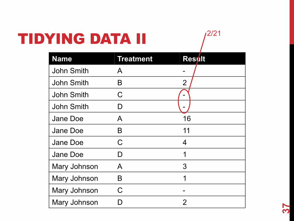
TIDYING DATA II
37
Name Treatment ResultJohn Smith A -John Smith B 2John Smith C -John Smith D -Jane Doe A 16Jane Doe B 11Jane Doe C 4Jane Doe D 1Mary Johnson A 3Mary Johnson B 1Mary Johnson C -Mary Johnson D 2
2/21

MELTING DATA I
38
religion <$10k $10-20k $20-30k $30-40k $40-50k $50-75k
Agnostic 27 34 60 81 76 137
Atheist 12 27 37 52 35 70
Buddhist 27 21 30 34 33 58
Catholic 418 617 732 670 638 1116
Dont know/refused 15 14 15 11 10 35
Evangelical Prot 575 869 1064 982 881 1486
Hindu 1 9 7 9 11 34
Historically Black Prot 228 244 236 238 197 223
Jehovahs Witness 20 27 24 24 21 30
Jewish 19 19 25 25 30 95
?????????????

MELTING DATA II
39
f_df = pd.melt(df,["religion"],var_name="income",value_name="freq")
f_df = f_df.sort_values(by=["religion"])f_df.head(10)
religion income freqAgnostic <$10k 27
Agnostic $30-40k 81
Agnostic $40-50k 76
Agnostic $50-75k 137
Agnostic $10-20k 34
Agnostic $20-30k 60
Atheist $40-50k 35
Atheist $20-30k 37
Atheist $10-20k 27
Atheist $30-40k 52

MORE COMPLICATED EXAMPLEBillboard Top 100 data for songs, covering their position on the Top 100 for 75 weeks, with two “messy” bits:• Column headers for each of the 75 weeks
• If a song didn’t last 75 weeks, those columns have are null
40
Thanks to http://jeannicholashould.com/tidy-data-in-python.html
year artist.inverted track time genre date.ente
reddate.peaked
x1st.week
x2nd.week ...
2000 Destiny's Child
Independent Women Part I 3:38 Rock 2000-09-
232000-11-18 78 63.0 ...
2000 Santana Maria, Maria 4:18 Rock 2000-02-12
2000-04-08 15 8.0 ...
2000 Savage Garden
I Knew I Loved You 4:07 Rock 1999-10-
232000-01-29 71 48.0 ...
2000 Madonna Music 3:45 Rock 2000-08-
122000-09-16 41 23.0 ...
2000 Aguilera, Christina
Come On Over Baby 3:38 Rock 2000-08-
052000-10-14 57 47.0 ...
2000 Janet Doesn't Really Matter 4:17 Rock 2000-06-
172000-08-26 59 52.0 ...
Messy columns!

MORE COMPLICATED EXAMPLE
Creates one row per week, per record, with its rank
41
# Keep identifier variablesid_vars = ["year",
"artist.inverted","track","time","genre","date.entered","date.peaked"]
# Melt the rest into week and rank columnsdf = pd.melt(frame=df,
id_vars=id_vars,var_name="week",value_name="rank")

42
MORE COMPLICATED EXAMPLE# Formattingdf["week"] = df['week'].str.extract('(\d+)’,
expand=False).astype(int)df["rank"] = df["rank"].astype(int)
# Cleaning out unnecessary rowsdf = df.dropna()
# Create "date" columnsdf['date'] = pd.to_datetime(
df['date.entered']) +pd.to_timedelta(df['week'], unit='w') –pd.DateOffset(weeks=1)
[…, “x2nd.week”, 63.0] à […, 2, 63]

MORE COMPLICATED EXAMPLE
43
# Ignore now-redundant, messy columnsdf = df[["year",
"artist.inverted","track","time","genre","week","rank","date"]]
df = df.sort_values(ascending=True,by=["year","artist.inverted","track","week","rank"])
# Keep tidy dataset for future usagebillboard = df
df.head(10)

MORE COMPLICATED EXAMPLE
44
year artist.inverted track time genre week rank date
2000 2 Pac Baby Don't Cry (Keep Ya Head Up II) 4:22 Rap 1 87 2000-02-26
2000 2 Pac Baby Don't Cry (Keep Ya Head Up II) 4:22 Rap 2 82 2000-03-04
2000 2 Pac Baby Don't Cry (Keep Ya Head Up II) 4:22 Rap 3 72 2000-03-11
2000 2 Pac Baby Don't Cry (Keep Ya Head Up II) 4:22 Rap 4 77 2000-03-18
2000 2 Pac Baby Don't Cry (Keep Ya Head Up II) 4:22 Rap 5 87 2000-03-25
2000 2 Pac Baby Don't Cry (Keep Ya Head Up II) 4:22 Rap 6 94 2000-04-01
2000 2 Pac Baby Don't Cry (Keep Ya Head Up II) 4:22 Rap 7 99 2000-04-08
2000 2Ge+herThe Hardest Part Of Breaking Up (Is
Getting Ba...3:15 R&B 1 91 2000-09-02
2000 2Ge+herThe Hardest Part Of Breaking Up (Is
Getting Ba...3:15 R&B 2 87 2000-09-09
2000 2Ge+herThe Hardest Part Of Breaking Up (Is
Getting Ba...3:15 R&B 3 92 2000-09-16
?????????????

MORE TO DO?Column headers are values, not variable names?• Good to go!
Multiple variables are stored in one column?• Maybe (depends on if genre text in raw data was multiple)
Variables are stored in both rows and columns?• Good to go!
Multiple types of observational units in the same table?• Good to go! One row per song’s week on the Top 100.
A single observational unit is stored in multiple tables?• Don’t do this!
Repetition of data?• Lots! Artist and song title’s text names. Which leads us to …
45

TODAY/NEXT CLASS§ Tables
§ Abstraction§ Operations
§ Pandas
§ Tidy Data
§ SQL and Relational Databases
46

TODAY’S LECTURERelational data:• What is a relation, and how do they interact?
Querying databases:• SQL
• SQLite• How does this relate to pandas?
Joins
47
Thanks to Zico Kolter for some structure for this lecture!

RELATIONSimplest relation: a table aka tabular data full of unique tuples
48
ID age wgt_kg hgt_cm
1 12.2 42.3 145.1
2 11.0 40.8 143.8
3 15.6 65.3 165.3
4 35.1 84.2 185.8
Labels
Observations(called tuples)
Variables(called attributes)
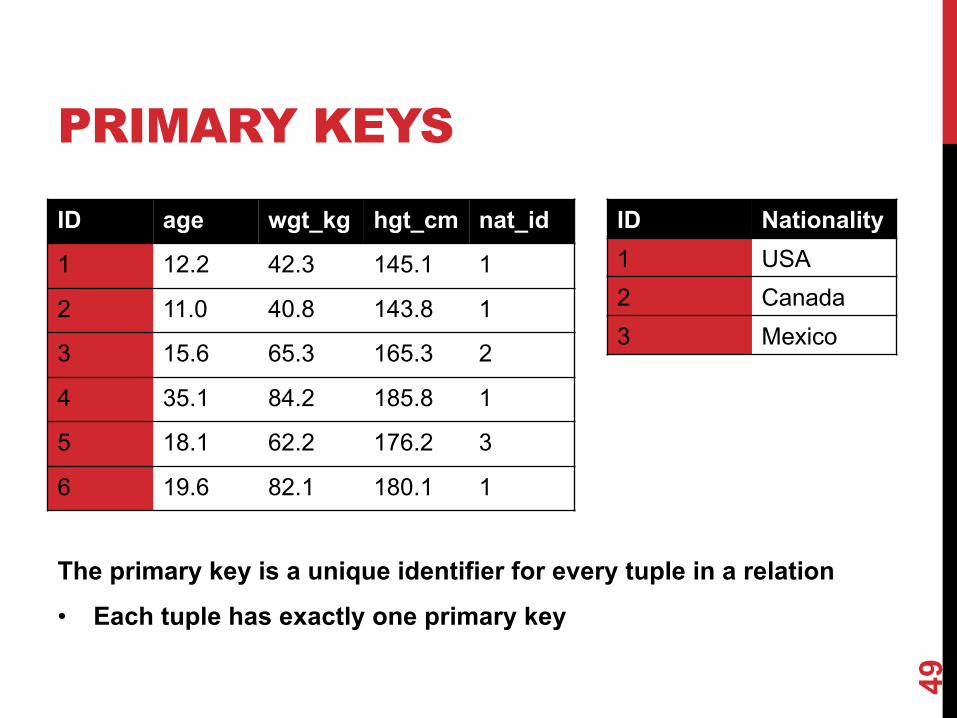
PRIMARY KEYS
The primary key is a unique identifier for every tuple in a relation
• Each tuple has exactly one primary key
49
ID age wgt_kg hgt_cm nat_id
1 12.2 42.3 145.1 1
2 11.0 40.8 143.8 1
3 15.6 65.3 165.3 2
4 35.1 84.2 185.8 1
5 18.1 62.2 176.2 3
6 19.6 82.1 180.1 1
ID Nationality1 USA2 Canada3 Mexico

FOREIGN KEYS
Foreign keys are attributes (columns) that point to a different table’s primary key• A table can have multiple foreign keys
50
ID age wgt_kg hgt_cm nat_id
1 12.2 42.3 145.1 1
2 11.0 40.8 143.8 1
3 15.6 65.3 165.3 2
4 35.1 84.2 185.8 1
5 18.1 62.2 176.2 3
6 19.6 82.1 180.1 1
ID Nationality1 USA2 Canada3 Mexico

SEARCHING FOR ELEMENTSFind all people with nationality Canada (nat_id = 2):
???????????????
51
ID age wgt_kg hgt_cm nat_id
1 12.2 42.3 145.1 1
2 11.0 40.8 143.8 1
3 15.6 65.3 165.3 2
4 35.1 84.2 185.8 1
5 18.1 62.2 176.2 3
6 19.6 82.1 180.1 1
O(n)

INDEXESLike a hidden sorted map of references to a specific attribute (column) in a table; allows O(log n) lookup instead of O(n)
52
loc ID age wgt_kg hgt_cm nat_id
0 1 12.2 42.3 145.1 1
128 2 11.0 40.8 143.8 2
256 3 15.6 65.3 165.3 2
384 4 35.1 84.2 185.8 1
512 5 18.1 62.2 176.2 3
640 6 19.6 82.1 180.1 1
nat_id locs1 0, 384,
6402 128, 2563 512

INDEXESActually implemented with data structures like B-trees• (Take courses like CMSC424 or CMSC420)
But: indexes are not free• Takes memory to store
• Takes time to build• Takes time to update (add/delete a row, update the column)
But, but: one index is (mostly) free• Index will be built automatically on the primary key
Think before you build/maintain an index on other attributes!
53

RELATIONSHIPSPrimary keys and foreign keys define interactions between different tables aka entities. Four types:• One-to-one
• One-to-one-or-none
• One-to-many and many-to-one
• Many-to-many
Connects (one, many) of the rows in one table to (one, many) of the rows in another table
54

ONE-TO-MANY & MANY-TO-ONEOne person can have one nationality in this example, but one nationality can include many people.
55
ID age wgt_kg hgt_cm nat_id
1 12.2 42.3 145.1 1
2 11.0 40.8 143.8 1
3 15.6 65.3 165.3 2
4 35.1 84.2 185.8 1
5 18.1 62.2 176.2 3
6 19.6 82.1 180.1 1
ID Nationality1 USA2 Canada3 Mexico
Person Nationality

ONE-TO-ONETwo tables have a one-to-one relationship if every tuple in the first tables corresponds to exactly one entry in the other
In general, you won’t be using these (why not just merge the rows into one table?) unless:• Split a big row between SSD and HDD or distributed
• Restrict access to part of a row (some DBMSs allow column-level access control, but not all)
• Caching, partitioning, & serious stuff: take CMSC424
56
Person SSN

ONE-TO-ONE-OR-NONESay we want to keep track of people’s cats:
People with IDs 2 and 3 do not own cats*, and are not in the table. Each person has at most one entry in the table.
Is this data tidy?
57
Person ID Cat1 Cat21 Chairman Meow Fuzz Aldrin4 Anderson Pooper Meowly Cyrus5 Gigabyte Megabyte
Person Cat
*nor do they have hearts, apparently.

MANY-TO-MANYSay we want to keep track of people’s cats’ colorings:
One column per color, too many columns, too many nullsEach cat can have many colors, and each color many cats
58
ID Name1 Megabyte2 Meowly Cyrus3 Fuzz Aldrin4 Chairman Meow5 Anderson Pooper6 Gigabyte
Cat ID Color ID Amount1 1 501 2 502 2 202 4 402 5 403 1 100
Cat Color

ASSOCIATIVE TABLES
Primary key ???????????• [Cat ID, Color ID] (+ [Color ID, Cat ID], case-dependent)
Foreign key(s) ???????????• Cat ID and Color ID
59
Cat ID Color ID Amount1 1 501 2 502 2 202 4 402 5 403 1 100
ID Name
1 Megabyte
2 Meowly Cyrus
3 Fuzz Aldrin
4 Chairman Meow
5 Anderson Pooper
6 Gigabyte
ID Name
1 Black
2 Brown
3 White
4 Orange
5 Neon Green
6 Invisible
Cats Colors

ASIDE: PANDASSo, this kinda feels like pandas …• And pandas kinda feels like a relational data system …
Pandas is not strictly a relational data system:• No notion of primary / foreign keys
It does have indexes (and multi-column indexes):• pandas.Index: ordered, sliceable set storing axis labels
• pandas.MultiIndex: hierarchical index
Rule of thumb: do heavy, rough lifting at the relational DB level, then fine-grained slicing and dicing and viz with pandas
60

SQLITEOn-disk relational database management system (RDMS)• Applications connect directly to a file
Most RDMSs have applications connect to a server:• Advantages include greater concurrency, less restrictive
locking
• Disadvantages include, for this class, setup time JInstallation:• conda install -c anaconda sqlite
• (Should come preinstalled, I think?)
All interactions use Structured Query Language (SQL)
61
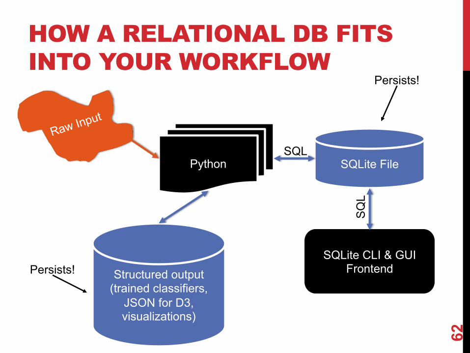
HOW A RELATIONAL DB FITS INTO YOUR WORKFLOW
62
SQLite CLI & GUI Frontend
SQLite FilePython
Raw Input
Structured output (trained classifiers,
JSON for D3, visualizations)
SQL
SQL
Persists!
Persists!

CRASH COURSE IN SQL (IN PYTHON)
Cursor: temporary work area in system memory for manipulating SQL statements and return valuesIf you do not close the connection (conn.close()), any outstanding transaction is rolled back• (More on this in a bit.)
63
import sqlite3
# Create a database and connect to itconn = sqlite3.connect(“cmsc320.db”)cursor = conn.cursor()
# do cool stuffconn.close()

CRASH COURSE IN SQL (IN PYTHON)
Capitalization doesn’t matter for SQL reserved words• SELECT = select = SeLeCtRule of thumb: capitalize keywords for readability 64
# Make a tablecursor.execute(“””CREATE TABLE cats (
id INTEGER PRIMARY KEY,name TEXT
)”””)
?????????
id namecats
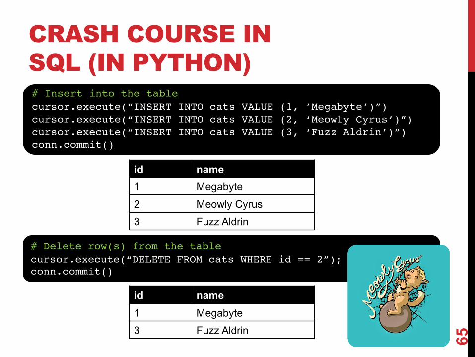
CRASH COURSE IN SQL (IN PYTHON)
65
# Insert into the tablecursor.execute(“INSERT INTO cats VALUE (1, ’Megabyte’)”)cursor.execute(“INSERT INTO cats VALUE (2, ‘Meowly Cyrus’)”)cursor.execute(“INSERT INTO cats VALUE (3, ‘Fuzz Aldrin’)”)conn.commit()
id name1 Megabyte2 Meowly Cyrus3 Fuzz Aldrin
# Delete row(s) from the tablecursor.execute(“DELETE FROM cats WHERE id == 2”);conn.commit()
id name1 Megabyte3 Fuzz Aldrin

CRASH COURSE IN SQL (IN PYTHON)
index_col=“id”: treat column with label “id” as an indexindex_col=1: treat column #1 (i.e., “name”) as an index(Can also do multi-indexing.)
66
# Read all rows from a tablefor row in cursor.execute(”SELECT * FROM cats”):
print(row)
# Read all rows into pandas DataFramepd.read_sql_query(“SELECT * FROM cats”, conn, index_col=”id”)
id name1 Megabyte3 Fuzz Aldrin

JOINING DATAA join operation merges two or more tables into a single relation. Different ways of doing this:• Inner• Left• Right• Full Outer
Join operations are done on columns that explicitly link the tables together
67

INNER JOINS
Inner join returns merged rows that share the same value in the column they are being joined on (id and cat_id).
68
id name1 Megabyte2 Meowly Cyrus3 Fuzz Aldrin4 Chairman Meow5 Anderson Pooper6 Gigabyte
cat_id last_visit1 02-16-20172 02-14-20175 02-03-2017
cats
visits
id name last_visit1 Megabyte 02-16-20172 Meowly Cyrus 02-14-20175 Anderson Pooper 02-03-2017
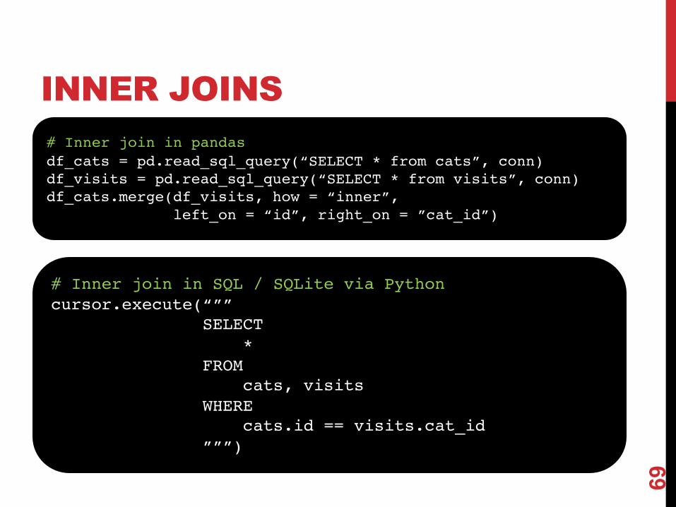
INNER JOINS
69
# Inner join in pandasdf_cats = pd.read_sql_query(“SELECT * from cats”, conn)df_visits = pd.read_sql_query(“SELECT * from visits”, conn)df_cats.merge(df_visits, how = “inner”,
left_on = “id”, right_on = ”cat_id”)
# Inner join in SQL / SQLite via Pythoncursor.execute(“””
SELECT *
FROM cats, visits
WHEREcats.id == visits.cat_id
”””)

LEFT JOINSInner joins are the most common type of joins (get results that appear in both tables)Left joins: all the results from the left table, only somematching results from the right tableLeft join (cats, visits) on (id, cat_id) ???????????
70
id name last_visit1 Megabyte 02-16-20172 Meowly Cyrus 02-14-20173 Fuzz Aldrin NULL4 Chairman Meow NULL5 Anderson Pooper 02-03-20176 Gigabyte NULL

RIGHT JOINSTake a guess!Right join
(cats, visits)on
(id, cat_id)???????????
71
id name1 Megabyte2 Meowly Cyrus3 Fuzz Aldrin4 Chairman Meow5 Anderson Pooper6 Gigabyte
cat_id last_visit1 02-16-20172 02-14-20175 02-03-20177 02-19-201712 02-21-2017
catsvisits
id name last_visit1 Megabyte 02-16-20172 Meowly Cyrus 02-14-20175 Anderson Pooper 02-03-20177 NULL 02-19-201712 NULL 02-21-2017

LEFT/RIGHT JOINS
72
# Left join in pandasdf_cats.merge(df_visits, how = “left”,
left_on = “id”, right_on = ”cat_id”)
# Right join in pandasdf_cats.merge(df_visits, how = “right”,
left_on = “id”, right_on = ”cat_id”)
# Left join in SQL / SQLite via Pythoncursor.execute(“SELECT * FROM cats LEFT JOIN visits ON
cats.id == visits.cat_id”)
# Right join in SQL / SQLite via PythonL

FULL OUTER JOINCombines the left and the right join ???????????
73
id name last_visit1 Megabyte 02-16-20172 Meowly Cyrus 02-14-20173 Fuzz Aldrin NULL4 Chairman Meow NULL5 Anderson Pooper 02-03-20176 Gigabyte NULL7 NULL 02-19-201712 NULL 02-21-2017
# Outer join in pandasdf_cats.merge(df_visits, how = “outer”,
left_on = “id”, right_on = ”cat_id”)

GOOGLE IMAGE SEARCH ONE SLIDE SQL JOIN VISUAL
74
Image credit: http://www.dofactory.com/sql/join

RAW SQL IN PANDASIf you “think in SQL” already, you’ll be fine with pandas:• conda install -c anaconda pandasql
• Info: http://pandas.pydata.org/pandas-docs/stable/comparison_with_sql.html
75
# Write the query textq = ”””
SELECT*
FROMcats
LIMIT 10;”””
# Store in a DataFramedf = sqldf(q, locals())

NEXT CLASS:EXPLORATORY ANALYSIS
76


