Introduction to Deep Learning - Ingegneria...

Sapienza University of Rome, Italy

University of Rome “La Sapienza”

Dep. of Computer, Control and Management Engineering A. Ruberti

Introduction to Deep Learning

Valsamis Ntouskos

ALCOR Lab

Valsamis Ntouskos (ALCOR Lab) Introduction to Deep Learning 1 / 39


Overview

Linear Classification

Logistic Regression

Linear Regression

Deep Feedforward Networks

Training DFNs

Activation Function

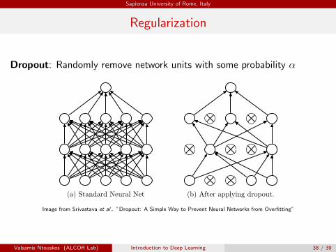
Regularization



Linear Models for Classification

Learning a function f : X → Y , with ...

X ⊆ <n

Y = {C1, . . . ,Ck}

assuming linearly separable data.



Linearly separable data

Instances in a data set are linearly separable iff it exists a hyperplane thatdivide the instance space into two regions such that differently classifiedinstances are separated.



Discriminant functions

Linear discriminant function

y : X → {C1, . . . ,CK}

Two classes:y(x) = wTx + w0

Multi classes:yk(x) = wT

k x + wk0



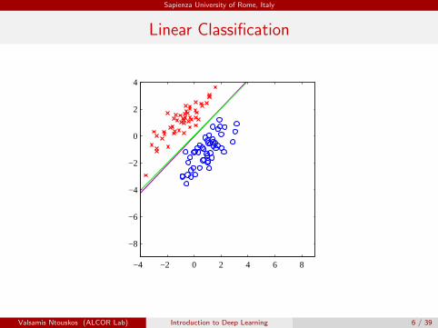
Linear Classification

−4 −2 0 2 4 6 8

−8

−6

−4

−2

0

2

4



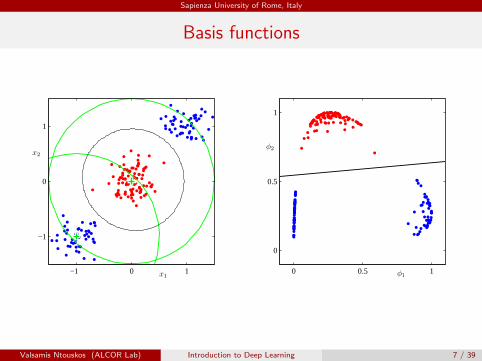
Basis functions

x1

x2

−1 0 1

−1

0

1

φ1

φ2

0 0.5 1

0

0.5

1



Logistic Regression

Consider first the case of two classes.

Find the conditional probability:

P(C1|x) =P(x|C1)P(C1)

P(x|C1)p(C1) + P(x|C2)p(C2)

=1

1 + exp(−α)= σ(α).

with:

α = ln P(x|C1)P(C1)P(x|C2)P(C2)

and

σ(α) = 11+exp(−α) the sigmoid function.



Logistic Regression

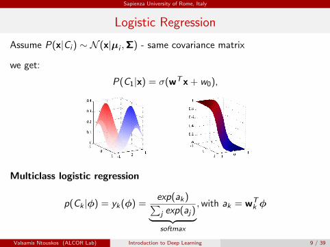
Assume P(x|Ci ) ∼ N (x|µi ,Σ) - same covariance matrix

we get:

P(C1|x) = σ(wTx + w0),

Multiclass logistic regression

p(Ck |φ) = yk(φ) =exp(ak)∑j exp(aj)︸︷︷︸softmax

,with ak = wTk φ



Linear Regression

Goal: Estimate the value t of a continuous function at x based on adataset D composed of N observations {xn}, where n = 1, . . . ,N,together with the corresponding target values {tn}.

Ideally:t = y(x,w)



Linear Regression - Model

Linear Basis Function Models

Simplest case:

y(x,w) = w0 + w1x1 + . . .+ wDxD = wTx

with x =

1...xD

and w =

w0...

wD

Linear both in model parameters w and variables x.

Too limiting!



Example - Line fitting

y = w1x1 + w0

−4 −3 −2 −1 0 1 2 3 4−3

−2

−1

0

1

2

3

4

5

predictiontruth




Linear Basis Function Models

Using nonlinear functions of input variables:

y(x,w) =M−1∑j=0

wjφj(x) = wTφ,

with φ0(x) = 1 and φ =

φ0...

φM−1

Still linear in the parameters w!



Example - Polynomial curve fitting

y = w0 + w1x + w2x2 + . . .+ wMxM =

M∑j=0

wjxj

x

t

M = 0

0 1

−1

0

1

x

t

M = 1

0 1

−1

0

1

x

t

M = 3

0 1

−1

0

1

x

t

M = 9

0 1

−1

0

1




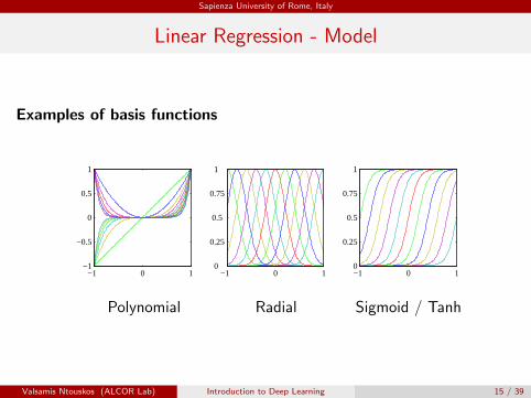
Examples of basis functions

−1 0 1−1

−0.5

0

0.5

1

−1 0 10

0.25

0.5

0.75

1

−1 0 10

0.25

0.5

0.75

1

Polynomial Radial Sigmoid / Tanh




Alternative names:

Feedforward Neural Networks

(Artificial) Neural Networks - (A)NNs

Multilayer Perceptrons - MLPs

Represent a parametric function

Suitable for tasks described as associating a vector to another vector




Goal: Estimate some function f ∗

Examples:

Classification y = f ∗(x) with x ∈ X and y ∈ {c1, . . . , cK}Regression y = f ∗(x) with x ∈ X and y ∈ R

Density estimation y = f ∗(x) with x ∈ X and∫X y = 1

Framework: Define y = f (x,θ) and learn parameters θ




Data: target values tn corresponding to given input variable values xnsuch that tn ≈ f ∗(xn)We use ≈ as the data may be affected by noise.

Objective:Learn θ such that f (x,θ) approximates as much as possible f ∗.Training based on a suitable cost (loss) function

Note: Dataset contains no target values about hidden units!



DFN - Terminology

Feedforward information flows from input to output without any loops

Networks f is a composition of elementary functions in an acyclic graph

Example:f (x) = f (3)(f (2)(f (1)(x,θ(1)),θ(2)),θ(3))

where:

f (m) the m-th layer of the network

and

θ(m) the corresponding parameters



DFN - Terminology

DFNs are chain structures

The length of the chain is the depth of the network

Final layer also called output layer

Name deep learning follows from the use of networks with a large numberof layers (large depth)




Draw inspiration from brain structures

Image from Isaac Changhau https://isaacchanghau.github.io

Hidden layer output can be seen as an array of unit (neuron) activationsbased on the connections with the previous units

Note: Only use some insights, they are not a model of the brain function!


https://isaacchanghau.github.io



Why DFNs?

Linear models cannot model interaction between input variables

Kernel methods require the choice of suitable kernels

use generic kernels e.g. RBF, polynomial, etc. (convex problem)

use hand-crafted kernels - application specific (convex problem)

Deep leaning:consider parametric mapping functions φ and learn their parameters(non-convex problem)

Model:y = f (x,θ,w) = φ(x,θ)Tw



Gradient-based learning

Learning remarks

Parameters found via gradient-based learning

Unit saturation can hinder learning

When units saturate gradient becomes very small

Suitable cost function and unit nonlinearities help to avoid saturation



Cost function

Model implicitly defines a conditional distribution p(t|x,θ)

Cost function:Typically choose the negative log-likelihood - Maximum likelihood principle

J(θ) = − ln(p(t|x))

Example:Assuming additive Gaussian noise we have

p(t|x) = N (t|f (x,θ), β−1I )

and hence

J(θ) =1

2(t− f (x,θ))2



Gradient Computation

Information flows forward throughthe network when computingnetwork output y from input x

To train the network we need tocompute the gradients with respectto the network parameters θ

The back-propagation or backpropalgorithm is used to propagategradient computation from the costthrough the whole network

Image by Y. LeCun



Gradient Computation

Goal: Compute the gradient of the cost function w.r.t. the parameters

∇θJ(θ)

Analytic computation of the gradient is straightforward

simple application of the chain rule

numerical evaluation can be expensive

Back-propagation is simple and inexpensive.

Remarks:

back-propagation is not a training algorithm

back-propagation is only used to compute the gradients

back-propagation is not specific to DFNs



Learning algorithms

Stochastic Gradient Descent (SGD)

SGD with momentum

Algorithms with adaptive learning rates



Stochastic Gradient Descent

Require: Learning rate ηRequire: Initial values of θk ← 1while stopping criterion not met do

Sample a subset (minibatch) {x(1), . . . , x(m)} of m examples from thedataset DCompute gradient estimate: g = 1

m∇θ∑

i L(f (x(i),θ), t(i))Apply update: θ ← θ − ηgk ← k + 1

end while

Note: η might change according to some rule through the iterations



Output units activation functions

Network output units determine also the cost function.Let h = f (x,θ) the output of the hidden layers.

RegressionLinear units: Identity activation function - no nonlinearity

y = W Th + b

Used to model a conditional Gaussian distribution

p(t|x) = N (t|y , β−1)

Maximum likelihood equivalent to minimizing mean squared error

Note: Linear units do not saturate!




Binary classificationSigmoid units: Sigmoid activation function

y = σ(wTh + b)

We have seen that the likelihood corresponds to a Bernoulli distributionHence:

J(θ) = − lnP(t|x)

= − lnσ(α)t(1− σ(α))1−t

= − lnσ((2t − 1)α)

= softplus((1− 2t)α),

with α = wTh + b.

Note: Unit saturates only when it gives the correct answer.If α has wrong sign softplus((1− 2t)α) ≈ |α| and dy

dα ≈ sign(α).Valsamis Ntouskos (ALCOR Lab) Introduction to Deep Learning 30 / 39



− −10 5 0 5 100

2

4

6

8

10ζx()

The softplus function




Multiclass classificationSoftmax units: Softmax activation function

y = softmax(α)i =exp(αi )∑

j αj

Likelihood corresponds to a Multinomial distributionHence:

J(θ)i = − ln softmax(α)i = ln∑j

exp(αj)− αi

Note: ln∑

j exp(αj) ≈ ln exp(maxj(αj)) = maxj αj .If αi corresponds to the correct answer the derivative is small.Misclassifications give large derivatives.



Hidden units activation functions

Rectified Linear Units:

g(α) = max{0, α}.

Easy to optimize - similar to linear units

Not differentiable at 0 - does not cause problems in practice



Hidden unit activation functions



Hidden unit activation functions

Sigmoid and hyperbolic tangent:

g(α) = σ(α)

andg(α) = tanh(α)

Closely related as tanh(α) = 2σ(2α)− 1.

Remarks:

No logarithm at the output, the units saturate easily.

Gradient based learning is very slow.

Hyperbolic tangent gives larger gradients with respect to the sigmoid.



Activation functions overview

Image from Geron A. ”Hands-On Machine Learning with Scikit-Learn and TensorFlow”, O’Reilly 2017



Regularization

Early stopping:Stop iterations early to avoid overfitting to the training set of data



Regularization

Dropout: Randomly remove network units with some probability α

(a) Standard Neural Net (b) After applying dropout.

Image from Srivastava et al.. ”Dropout: A Simple Way to Prevent Neural Networks from Overfitting”



Regularization

With dropout

Without dropout

Image from Srivastava et al.. ”Dropout: A Simple Way to Prevent Neural Networks from Overfitting”


Date post:	22-May-2020
Category:	Documents
Upload:	others
View:	14 times
Download:	0 times

Introduction to Deep Learning - Ingegneria...

Documents