56
Introduction to diffraction and the Rietveld method Luca Lutterotti Corso: Laboratorio Scienza e Tecnologia dei MAteriali [email protected]
Introduction to diffraction and the
Rietveld methodLuca Lutterotti
Corso: Laboratorio Scienza e Tecnologia dei MAteriali
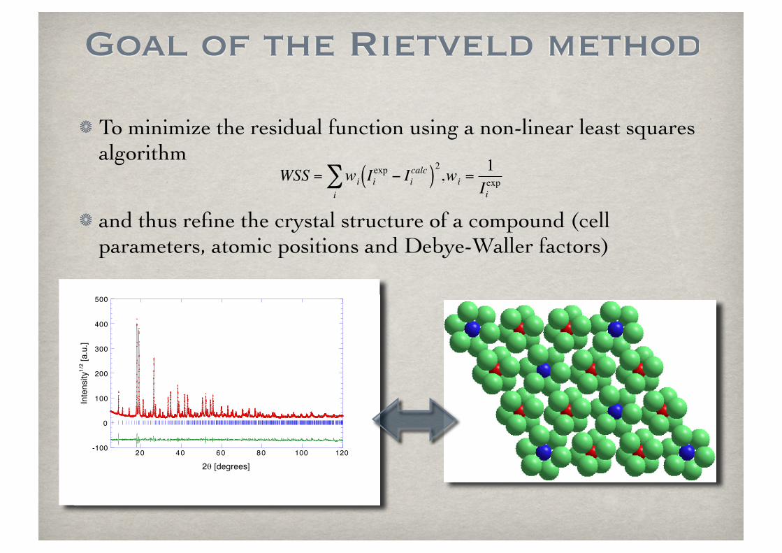
To minimize the residual function using a non-linear least squares algorithm
and thus refine the crystal structure of a compound (cell parameters, atomic positions and Debye-Waller factors)
Goal of the Rietveld method
€
WSS = wi Iiexp − Ii
calc( )2
i∑ ,wi =
1Iiexp
-100
0
100
200
300
400
500
20 40 60 80 100 120
Inte
nsity
1/2 [a
.u.]
2θ [degrees]
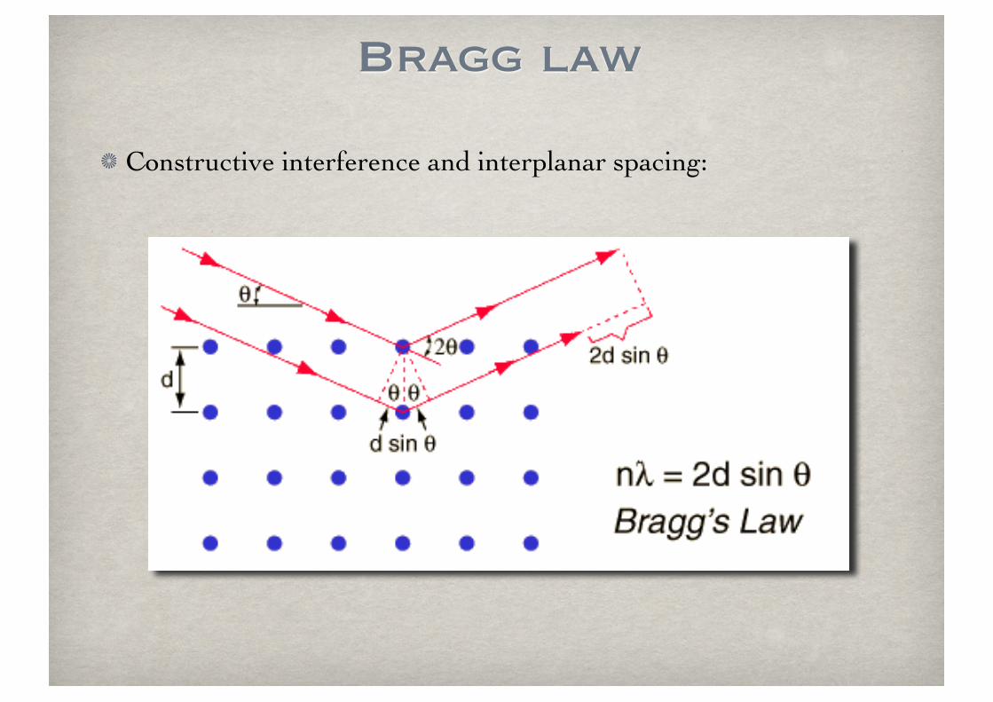
Bragg law
Constructive interference and interplanar spacing:
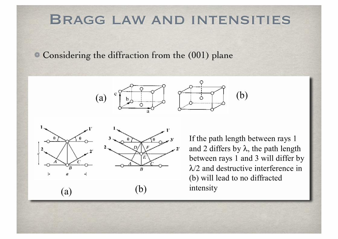
Bragg law and intensities
Considering the diffraction from the (001) plane
!"# !$#
!"# !$#
%&'()*'+"()',*-.()'$*(/**-'0"12'3'
"-4'5'46&&*02'$1'!7'()*'+"()',*-.()'$*(/**-'0"12'3'"-4'8'/6,,'46&&*0'$1'
!95'"-4'4*2(0:;(6<*'6-(*0&*0*-;*'6-'!$#'/6,,',*"4'(='-='46&&0";(*4'
6-(*-26(1
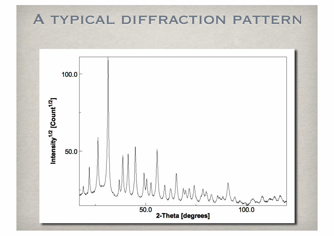
A typical diffraction pattern
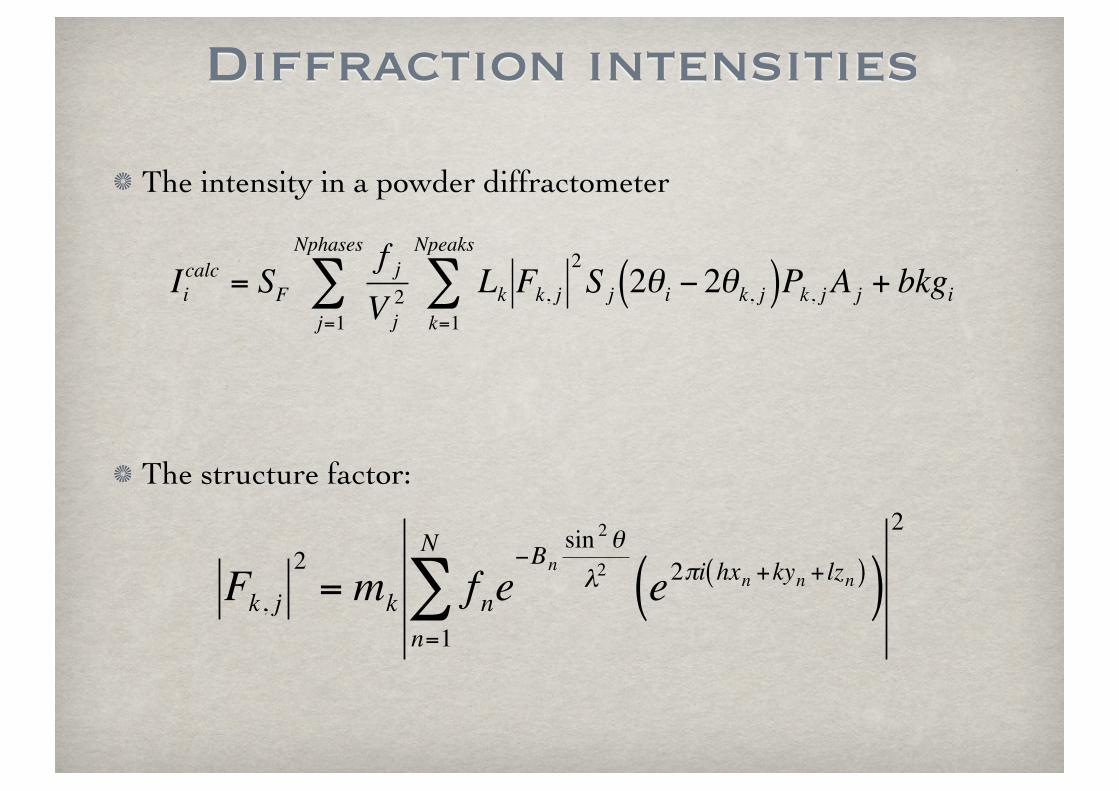
Diffraction intensities
The intensity in a powder diffractometer
The structure factor:€
Iicalc = SF
f jV j2 Lk Fk, j
2S j 2θi − 2θk, j( )Pk, j A j + bkgi
k=1
Npeaks
∑j=1
Nphases
∑
€
Fk, j2
= mk fne−Bn
sin 2θλ2 e2πi hxn +kyn + lzn( )( )
n=1
N
∑2
Diffraction analyses
Phase identifications (crystalline and amorphous)
Crystal structure determination
Crystal structure refinements
Quantitative phase analysis (and crystallinity determination)
Microstructural analyses (crystallite sizes - microstrain)
Texture analysis
Residual stress analysis
Order-disorder transitions and compositional analyses
Thin films
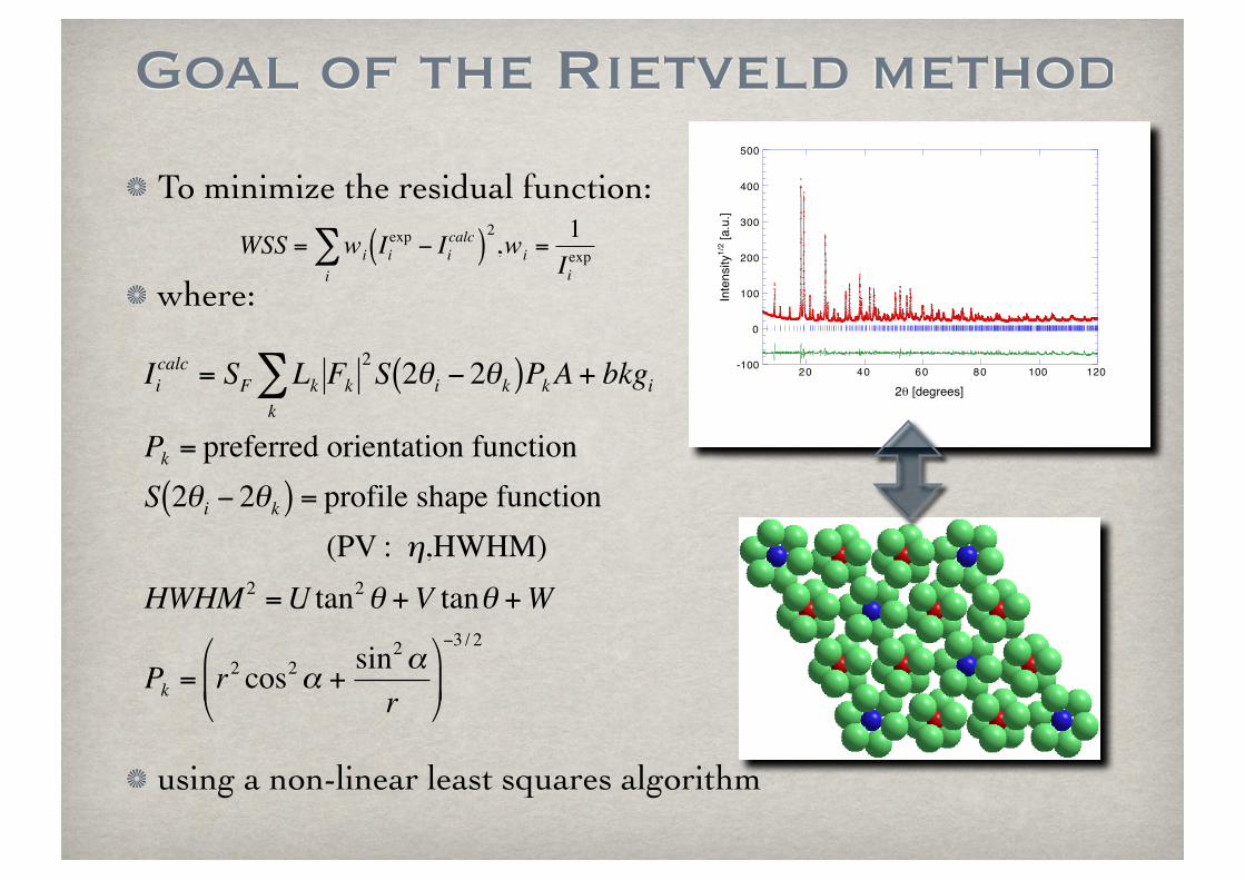
To minimize the residual function:
where:
using a non-linear least squares algorithm
Goal of the Rietveld method
€
WSS = wi Iiexp − Ii
calc( )2
i∑ ,wi =
1Iiexp
€
Iicalc = SF Lk Fk
2S 2θi − 2θk( )PkA + bkgik∑
Pk = preferred orientation functionS 2θi − 2θk( ) = profile shape function (PV : η,HWHM)HWHM 2 =U tan2θ +V tanθ +W
Pk = r2 cos2α +sin2αr
−3 / 2
-100
0
100
200
300
400
500
20 40 60 80 100 120
Inte
nsity
1/2 [a
.u.]
2θ [degrees]
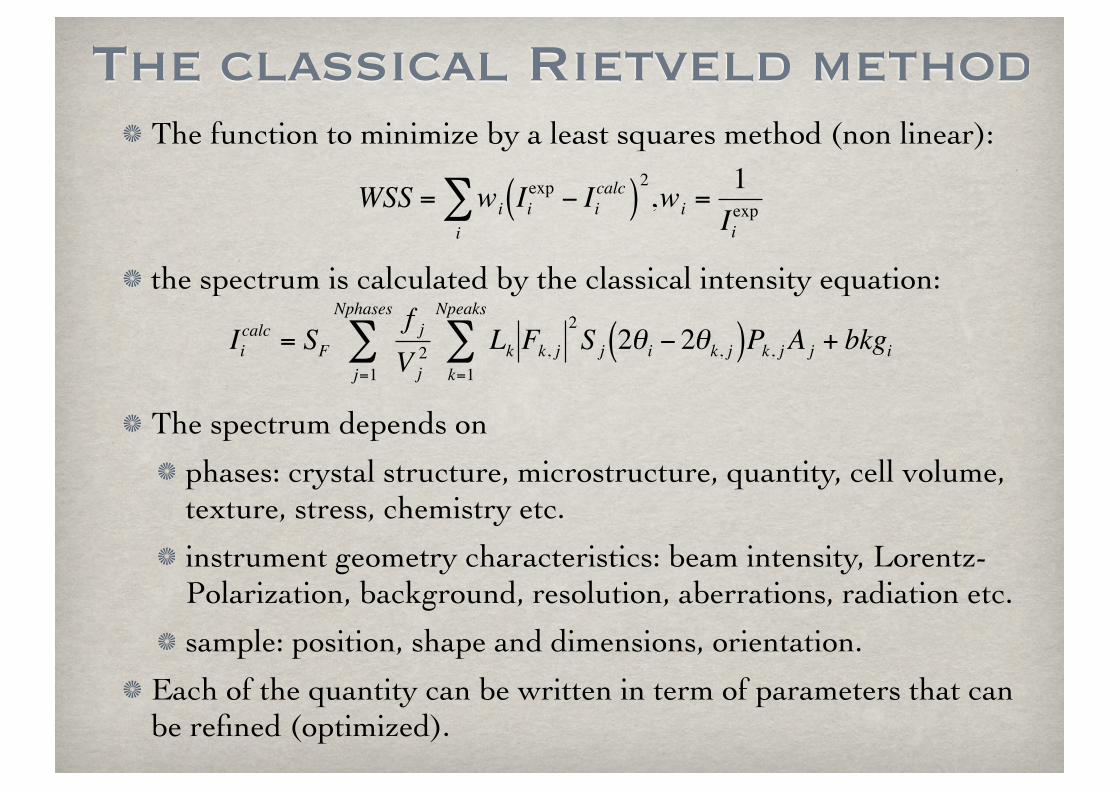
The classical Rietveld methodThe function to minimize by a least squares method (non linear):
the spectrum is calculated by the classical intensity equation:
The spectrum depends on
phases: crystal structure, microstructure, quantity, cell volume, texture, stress, chemistry etc.
instrument geometry characteristics: beam intensity, Lorentz-Polarization, background, resolution, aberrations, radiation etc.
sample: position, shape and dimensions, orientation.
Each of the quantity can be written in term of parameters that can be refined (optimized).
€
Iicalc = SF
f jV j2 Lk Fk, j
2S j 2θi − 2θk, j( )Pk, j A j + bkgi
k=1
Npeaks
∑j=1
Nphases
∑€
WSS = wi Iiexp − Ii
calc( )2
i∑ ,wi =
1Iiexp
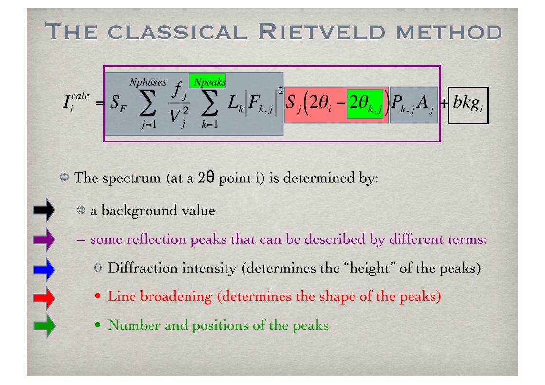
The spectrum (at a 2θ point i) is determined by:
a background value
– some reflection peaks that can be described by different terms:
Diffraction intensity (determines the “height” of the peaks)
• Line broadening (determines the shape of the peaks)
• Number and positions of the peaks
The classical Rietveld method
€
Iicalc = SF
f jV j2 Lk Fk, j
2S j 2θi − 2θk, j( )Pk, j A j + bkgi
k=1
Npeaks
∑j=1
Nphases
∑
The classical Rietveld method
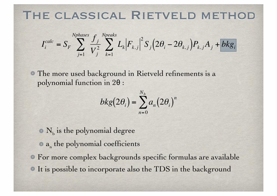
The more used background in Rietveld refinements is a polynomial function in 2θ :
Nb is the polynomial degree
an the polynomial coefficients
For more complex backgrounds specific formulas are available
It is possible to incorporate also the TDS in the background
€
Iicalc = SF
f jV j2 Lk Fk, j
2S j 2θi − 2θk, j( )Pk, j A j + bkgi
k=1
Npeaks
∑j=1
Nphases
∑
€
bkg 2θi( ) = an 2θi( )nn= 0
Nb
∑
The classical Rietveld method
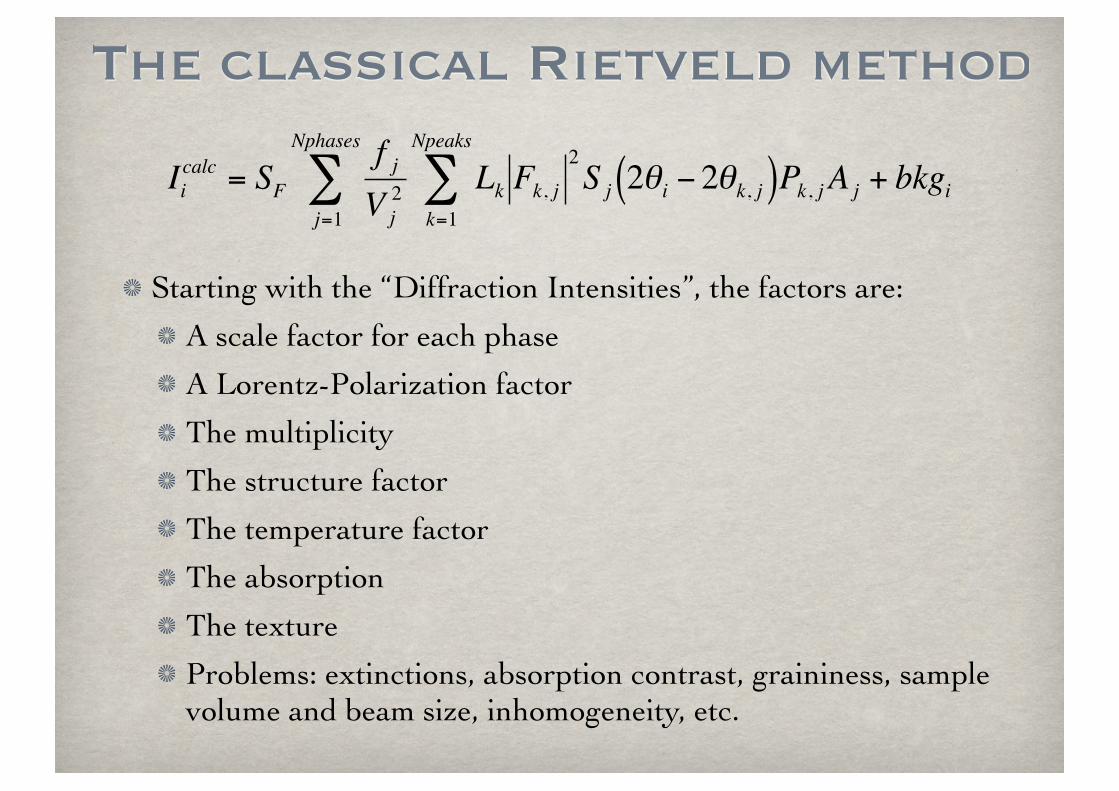
Starting with the “Diffraction Intensities”, the factors are:
A scale factor for each phase
A Lorentz-Polarization factor
The multiplicity
The structure factor
The temperature factor
The absorption
The texture
Problems: extinctions, absorption contrast, graininess, sample volume and beam size, inhomogeneity, etc.
€
Iicalc = SF
f jV j2 Lk Fk, j
2S j 2θi − 2θk, j( )Pk, j A j + bkgi
k=1
Npeaks
∑j=1
Nphases
∑
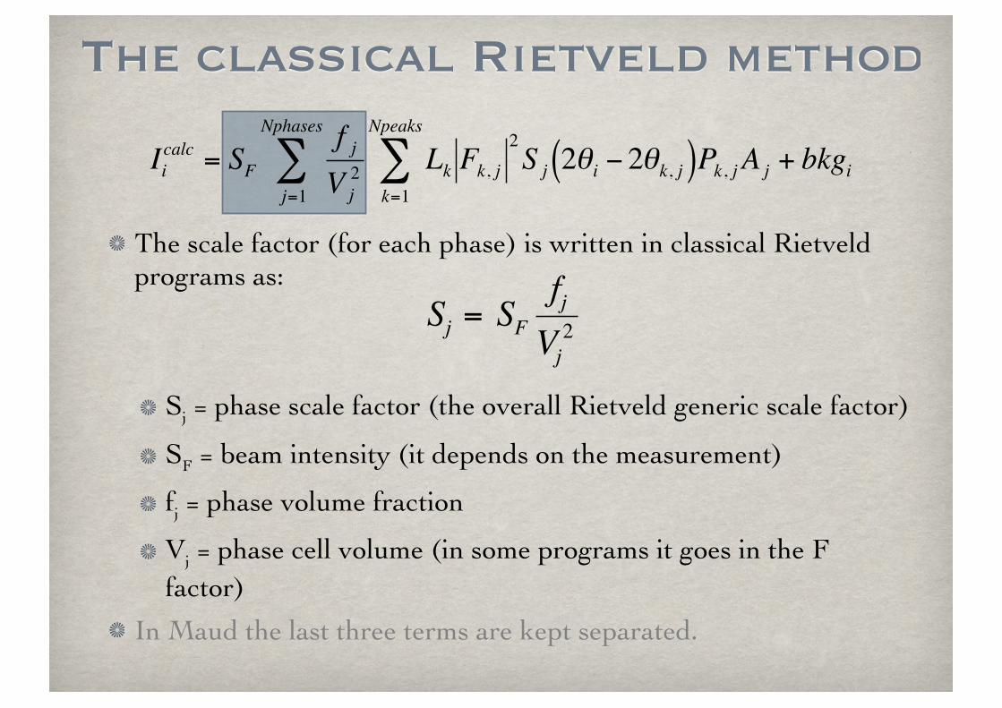
The classical Rietveld method
The scale factor (for each phase) is written in classical Rietveld programs as:
Sj = phase scale factor (the overall Rietveld generic scale factor)
SF = beam intensity (it depends on the measurement)
fj = phase volume fraction
Vj = phase cell volume (in some programs it goes in the F factor)
In Maud the last three terms are kept separated.
€
Sj = SFfjVj2€
Iicalc = SF
f jV j2 Lk Fk, j
2S j 2θi − 2θk, j( )Pk, j A j + bkgi
k=1
Npeaks
∑j=1
Nphases
∑
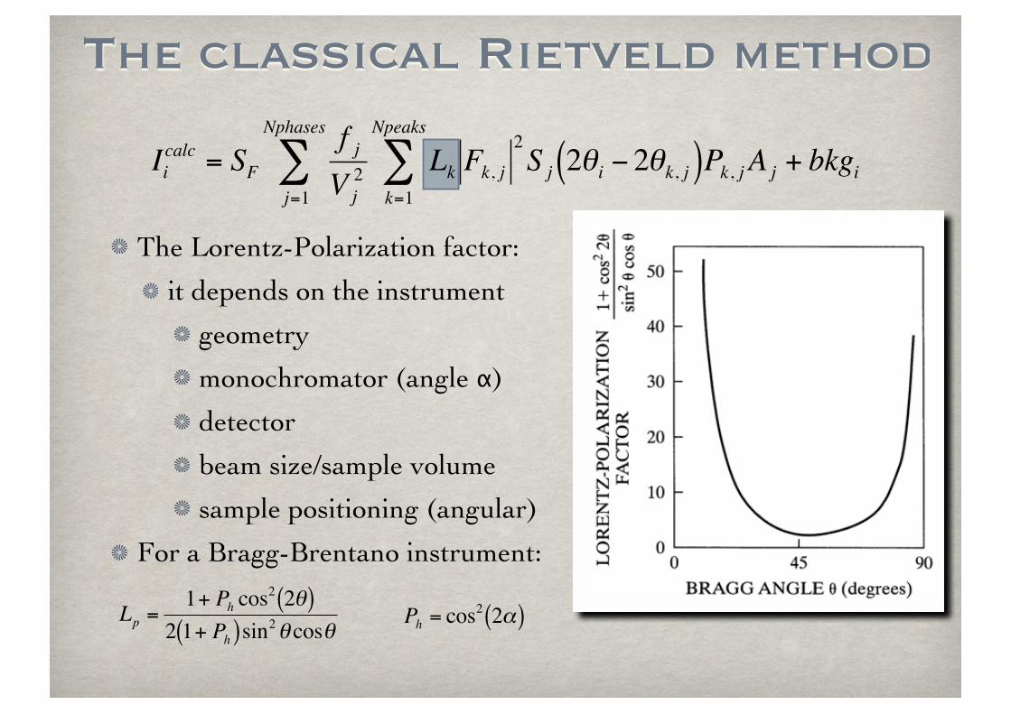
The classical Rietveld method
The Lorentz-Polarization factor:
it depends on the instrument
geometry
monochromator (angle α)
detector
beam size/sample volume
sample positioning (angular)
For a Bragg-Brentano instrument:
€
Iicalc = SF
f jV j2 Lk Fk, j
2S j 2θi − 2θk, j( )Pk, j A j + bkgi
k=1
Npeaks
∑j=1
Nphases
∑
€
Lp =1+ Ph cos
2 2θ( )2 1+ Ph( )sin2θ cosθ
€
Ph = cos2 2α( )
The classical Rietveld method
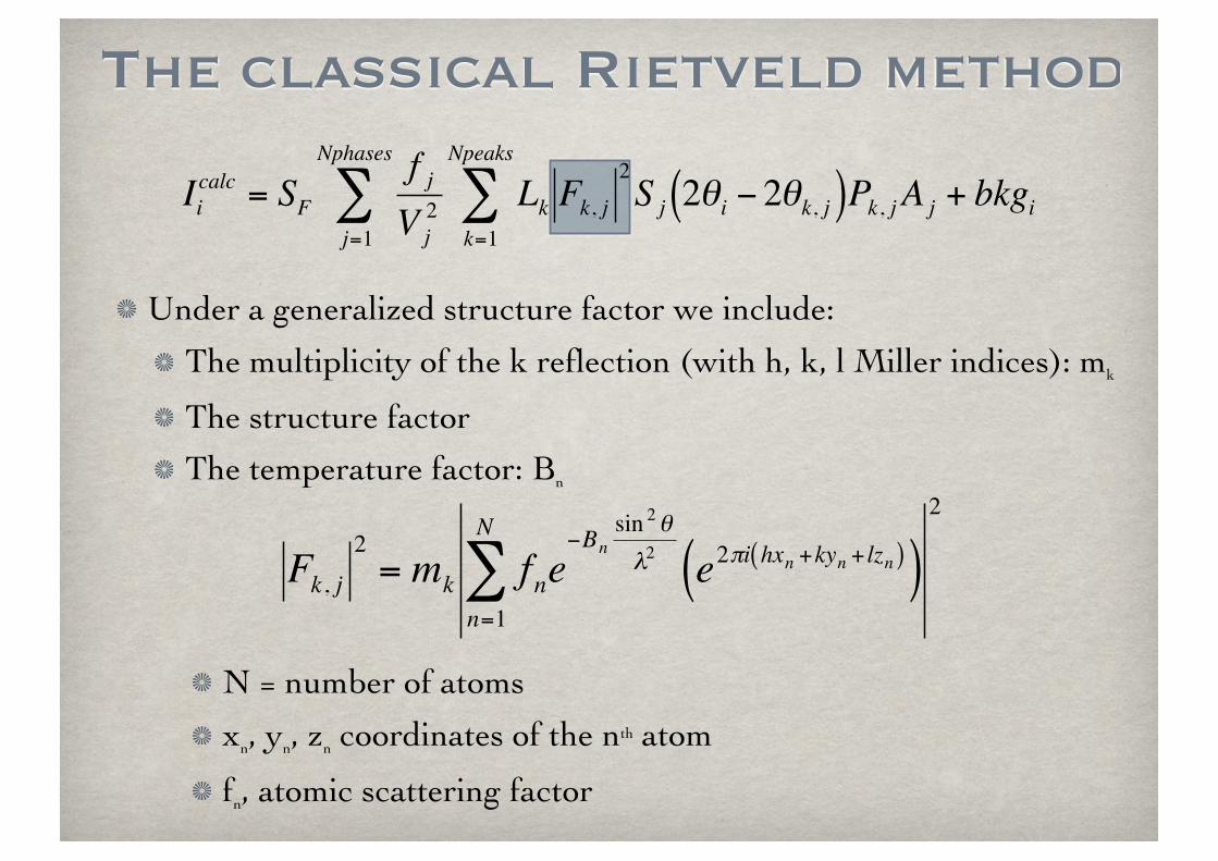
Under a generalized structure factor we include:
The multiplicity of the k reflection (with h, k, l Miller indices): mk
The structure factor
The temperature factor: Bn
N = number of atoms
xn, yn, zn coordinates of the nth atom
fn, atomic scattering factor
€
Iicalc = SF
f jV j2 Lk Fk, j
2S j 2θi − 2θk, j( )Pk, j A j + bkgi
k=1
Npeaks
∑j=1
Nphases
∑
€
Fk, j2
= mk fne−Bn
sin 2θλ2 e2πi hxn +kyn + lzn( )( )
n=1
N
∑2
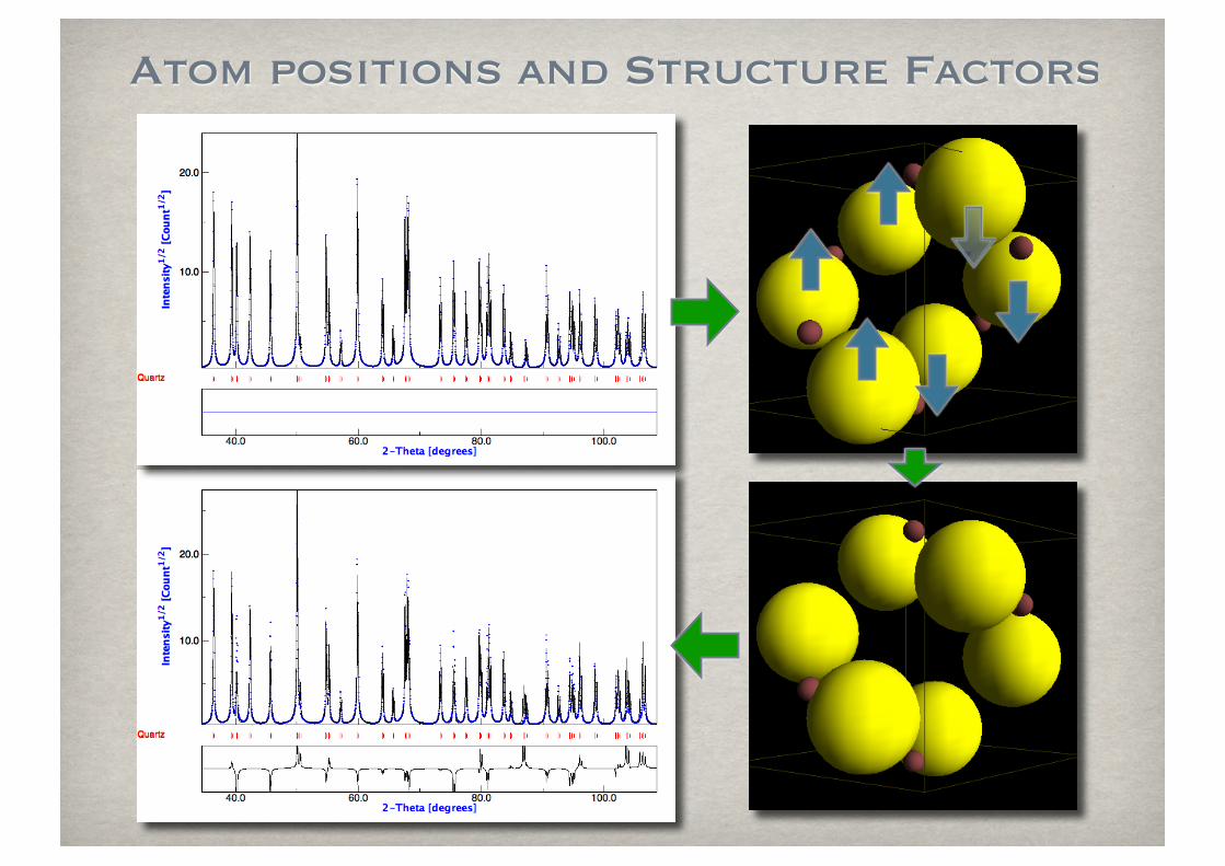
Atom positions and Structure Factors

Atomic scattering factor and Debye-Waller
The atomic scattering factor for X-ray decreases with the diffraction angle and is proportional to the number of electrons.
The temperature factor (Debye-Waller, B) accelerates the decrease.
The classical Rietveld method
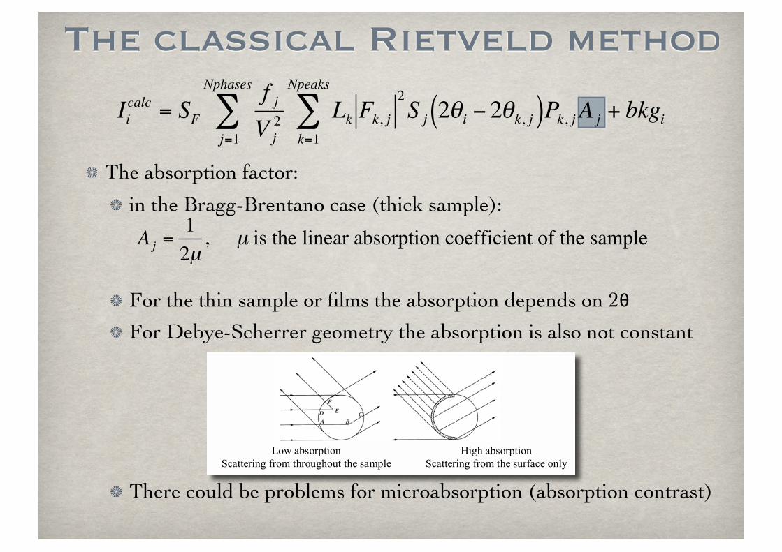
The absorption factor:
in the Bragg-Brentano case (thick sample):
For the thin sample or films the absorption depends on 2θ
For Debye-Scherrer geometry the absorption is also not constant
There could be problems for microabsorption (absorption contrast)
€
Iicalc = SF
f jV j2 Lk Fk, j
2S j 2θi − 2θk, j( )Pk, j A j + bkgi
k=1
Npeaks
∑j=1
Nphases
∑
!"#$%&'"()*+",-.%**/(+,0$1("2$*3("403"4*$*3/$'%2)5/
6+03$%&'"()*+",-.%**/(+,0$1("2$*3/$'4(1%./$",57
€
A j =1
2µ, µ is the linear absorption coefficient of the sample
The classical Rietveld method
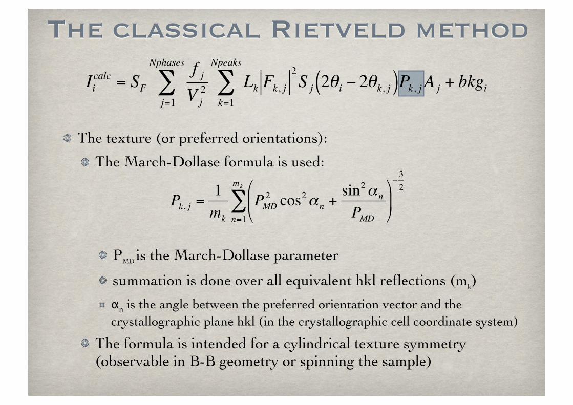
The texture (or preferred orientations):
The March-Dollase formula is used:
PMD is the March-Dollase parameter
summation is done over all equivalent hkl reflections (mk)
αn is the angle between the preferred orientation vector and the crystallographic plane hkl (in the crystallographic cell coordinate system)
The formula is intended for a cylindrical texture symmetry (observable in B-B geometry or spinning the sample)
€
Iicalc = SF
f jV j2 Lk Fk, j
2S j 2θi − 2θk, j( )Pk, j A j + bkgi
k=1
Npeaks
∑j=1
Nphases
∑
€
Pk, j =1mk
PMD2 cos2αn +
sin2αn
PMD
n=1
mk
∑−32
The classical Rietveld method
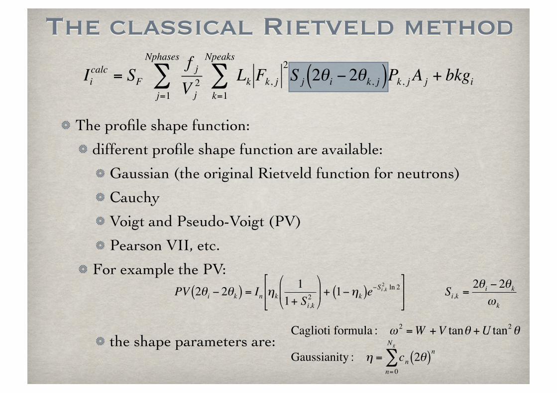
The profile shape function:
different profile shape function are available:
Gaussian (the original Rietveld function for neutrons)
Cauchy
Voigt and Pseudo-Voigt (PV)
Pearson VII, etc.
For example the PV:
the shape parameters are:
€
Iicalc = SF
f jV j2 Lk Fk, j
2S j 2θi − 2θk, j( )Pk, j A j + bkgi
k=1
Npeaks
∑j=1
Nphases
∑
€
Gaussianity : η = cn 2θ( )nn= 0
Ng
∑€
PV 2θi − 2θk( ) = In ηk1
1+ Si,k2
+ 1−ηk( )e−Si ,k
2 ln 2
Si,k =
2θi − 2θkωk
€
Caglioti formula : ω 2 =W +V tanθ +U tan2θ
The classical Rietveld method
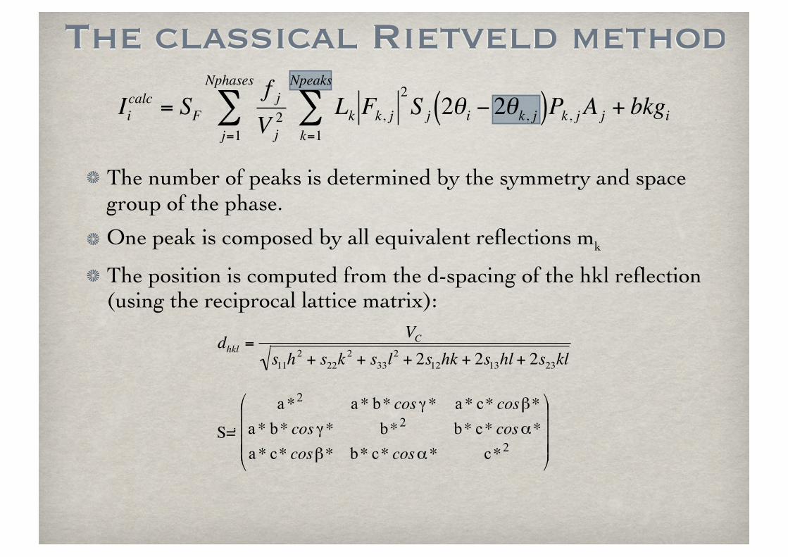
The number of peaks is determined by the symmetry and space group of the phase.
One peak is composed by all equivalent reflections mk
The position is computed from the d-spacing of the hkl reflection (using the reciprocal lattice matrix):
€
Iicalc = SF
f jV j2 Lk Fk, j
2S j 2θi − 2θk, j( )Pk, j A j + bkgi
k=1
Npeaks
∑j=1
Nphases
∑
€
dhkl =VC
s11h2 + s22k
2 + s33l2 + 2s12hk + 2s13hl + 2s23kl
1/19/01 GSAS TECHNICAL MANUAL PAGE 145
!"#$%#&'()$*%$%+*!,-.#$/'0$120,3$)*//0,&!'4#!#0%$5*!"$,$4'('&"0'4,!'0$*($6,0,..#.$
7#'4#!03$
!!
+!=
cossin
cos
8
8" 98:
; $
5"#0#$:"$*%$,$0#/*(,-.#$6'.,0*<,!*'($/0,&!*'($)#/*(#)$/'0$#,&"$120,3$6'5)#0$"*%!'70,4=$
>"#%#$/+(&!*'(%$",?#$%.*7"!.3$)*//#0#(!$/'04%$-+!$,0#$4,!"#4,!*&,..3$*)#(!*&,.=$@$!"*0)$
'6!*'($*%$!'$,66.3$('$;'0#(!<$,()$6'.,0*<,!*'($&'00#&!*'(%$!'$!"#$),!,$0#,)$*(!'$GSAS=$
>"*%$*%$+%#/+.$*/$!"#$6'5)#0$60'/*.#$),!,$5,%$&'00#&!#)$/'0$!"#%#$#//#&!%$-#/'0#$*(6+!$!'$
GSAS=$A)*!*(7$'/$!"#$;'0#(!<$,()$6'.,0*<,!*'($&'00#&!*'($*%$)'(#$*($EDTDIFS=$B($
GENLES$*(6+!$,()$'+!6+!$'/$!"#$:"$&'#//*&*#(!$*%$*($DIFSINP$,()$DIFSOUTC$!"#$;6$
&'00#&!*'($*%$&,.&+.,!#)$*($DIFSCAL=$
Reflection d-spacing and lattice parameters
>"#$)2%6,&*(7$/'0$,$0#/.#&!*'(D$hEF"DGD.HD$*%$7*?#($-3$!"#$%!,(),0)$#160#%%*'($
IG.8A".8J"G8K.LG@")9 8888 +++++== hgh $
5"#0#$7$*%$!"#$0#&*60'&,.$4#!0*&$!#(%'0$
""""
#
$
%%%%
&
'
()
(*
)*
=8
8
8
&&-&,
&---,
&,-,,
7
**cos***cos**
*cos****cos**
*cos***cos***
$
5"*&"$*%$!"#$*(?#0%#$'/$!"#$4#!0*&$!#(%'0$
""""
#
$
%%%%
&
'
()
(*
)*
=8
8
8
&-&,&
-&-,-
,&,-,
M
coscos
coscos
coscos
$
>"#$0#/*(#)$&'#//*&*#(!%$/'0$,$6'5)#0$)*//0,&!*'($6,!!#0($,0#$!"#$0#&*60'&,.$4#!0*&$!#(%'0$
#.#4#(!%$@2ID$,%$,..'5#)$-3$%344#!03=$A)*!*(7$'/$.,!!*&#$6,0,4#!#0%$*%$)'(#$-3$
EDTLAT$,()$*(6+!D$'+!6+!$,()$&,.&+.,!*'(%$*($GENLES$,0#$)'(#$-3$CELLINPD$
KA;;NO>D$CELLESD$,()$CELLCAL=$
Profile peak shape function
>"#$&'(!0*-+!*'($,$7*?#($0#/.#&!*'($4,G#%$!'$!"#$!'!,.$60'/*.#$*(!#(%*!3$)#6#()%$'($!"#$
%",6#$/+(&!*'($/'0$!",!$0#/.#&!*'($60'/*.#D$*!%$5*)!"$&'#//*&*#(!%$,()$!"#$)*%6.,#(!$'/$
!"#$6#,G$/0'4$!"#$60'/*.#$6'%*!*'(=$>"#$.'&,!*'(%$'/$!"#$6#,G$,0#$7*?#($*($4*&0'%#&'()%$'/$
>NID$&#(!*)#70##%$8!$'0$G#P=$J*%&+%%*'($'/$!"#%#$?,.+#%$*%$7*?#($/*0%!$/'..'5#)$-3$)#!,*.%$'/$!"#$6#,G$%",6#$/+(&!*'(%$60#%#(!.3$*(%!,..#)$*($GSAS=$
Neutron time of flight
I'0$,$(#+!0'($!*4#2'/2/.*7"!$6'5)#0$)*//0,&!'4#!#0$!"#$0#.,!*'(%"*6$-#!5##($!"#$)2%6,&*(7$
/'0$,$6,0!*&+.,0$6'5)#0$.*(#$,()$*!%$>NI$*%$
S=
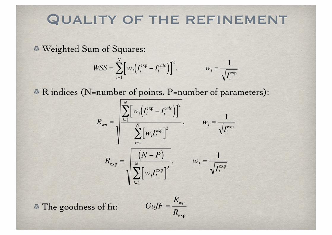
Quality of the refinement
Weighted Sum of Squares:
R indices (N=number of points, P=number of parameters):
The goodness of fit:
€
WSS = wi Iiexp − Ii
calc( )[ ]2
i=1
N
∑ , wi =1Ii
exp
€
Rwp =
wi Iiexp − Ii
calc( )[ ]2
i=1
N
∑
wiIiexp[ ]
2
i=1
N
∑, wi =
1Ii
exp
€
Rexp =N − P( )
wiIiexp[ ]
2
i=1
N
∑, wi =
1Ii
exp
€
GofF =Rwp
Rexp
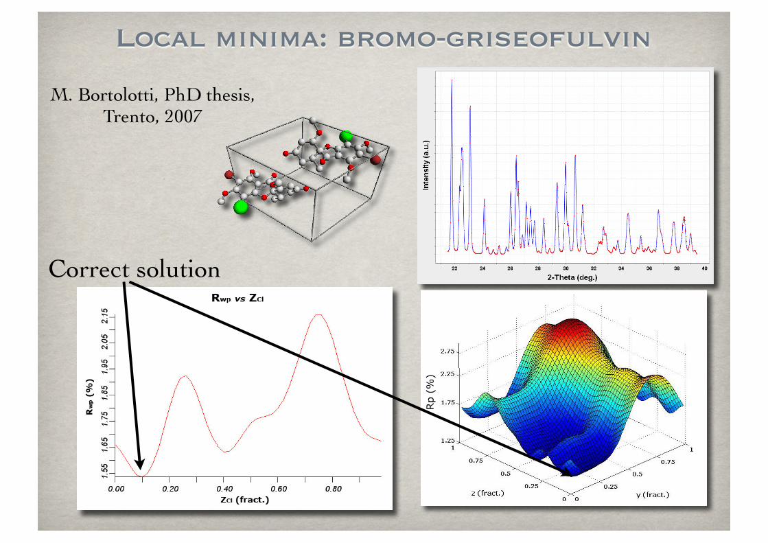
Local minima: bromo-griseofulvin
!
!
Correct solution
M. Bortolotti, PhD thesis, Trento, 2007
The R indices
The Rwp factor is the more valuable. Its absolute value does not depend on the absolute value of the intensities. But it depends on the background. With a high background is more easy to reach very low values. Increasing the number of peaks (sharp peaks) is more difficult to get a good value.
Rwp < 0.1 correspond to an acceptable refinement with a medium complex phase
For a complex phase (monoclinic to triclinic) a value < 0.15 is good
For a highly symmetric compound (cubic) with few peaks a value < 0.08 start to be acceptable
With high background better to look at the Rwp background subtracted.
The Rexp is the minimum Rwp value reachable using a certain number of refineable parameters. It needs a valid weighting scheme to be reliable.
WSS and GofF (or sigma)
The weighted sum of squares is only used for the minimization routines. Its absolute value depends on the intensities and number of points.
The goodness of fit is the ratio between the Rwp and Rexp and cannot be lower then 1 (unless the weighting scheme is not correctly valuable: for example in the case of detectors not recording exactly the number of photons or neutrons).
A good refinement gives GofF values lower than 2.
The goodness of fit is not a very good index to look at as with a noisy pattern is quite easy to reach a value near 1.
With very high intensities and low noise patterns is difficult to reach a value of 2.
The GofF is sensible to model inaccuracies.

Why the Rietveld refinement is widely used?
Pro
It uses directly the measured intensities points
It uses the entire spectrum (as wide as possible)
Less sensible to model errors
Less sensible to experimental errors
Cons
It requires a model
It needs a wide spectrum
– Rietveld programs are not easy to use
– Rietveld refinements require some experience (1-2 years?)
Can be enhanced by:
More automatic/expert mode of operation
Better easy to use programs
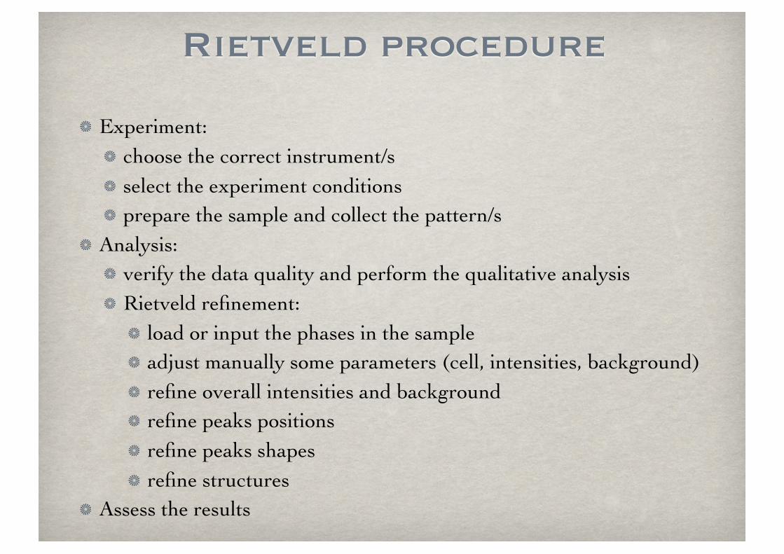
Rietveld procedure
Experiment:choose the correct instrument/sselect the experiment conditionsprepare the sample and collect the pattern/s
Analysis:verify the data quality and perform the qualitative analysisRietveld refinement:
load or input the phases in the sampleadjust manually some parameters (cell, intensities, background)refine overall intensities and backgroundrefine peaks positionsrefine peaks shapesrefine structures
Assess the results
Rietveld refinement procedure
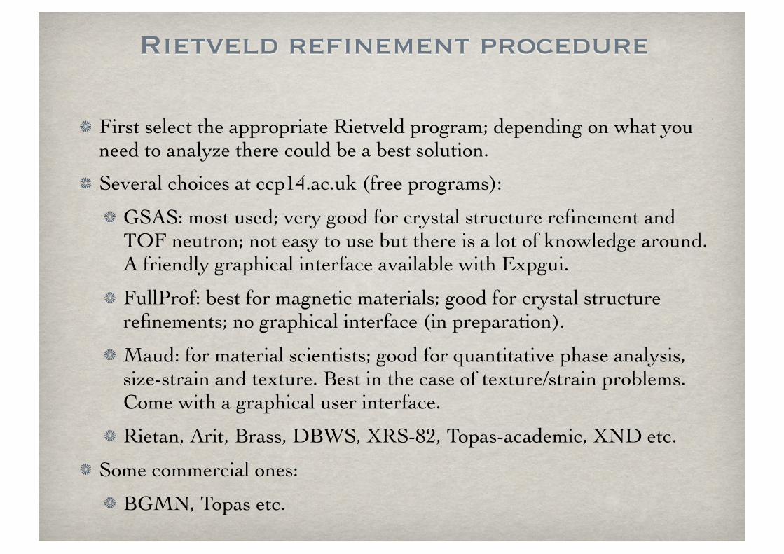
First select the appropriate Rietveld program; depending on what you need to analyze there could be a best solution.
Several choices at ccp14.ac.uk (free programs):
GSAS: most used; very good for crystal structure refinement and TOF neutron; not easy to use but there is a lot of knowledge around. A friendly graphical interface available with Expgui.
FullProf: best for magnetic materials; good for crystal structure refinements; no graphical interface (in preparation).
Maud: for material scientists; good for quantitative phase analysis, size-strain and texture. Best in the case of texture/strain problems. Come with a graphical user interface.
Rietan, Arit, Brass, DBWS, XRS-82, Topas-academic, XND etc.
Some commercial ones:
BGMN, Topas etc.

Starting point: defining the phases
We need to specify which phases we will work with (databases)
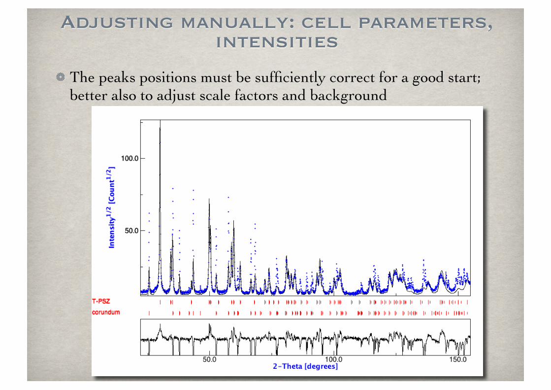
Adjusting manually: cell parameters, intensities
The peaks positions must be sufficiently correct for a good start; better also to adjust scale factors and background
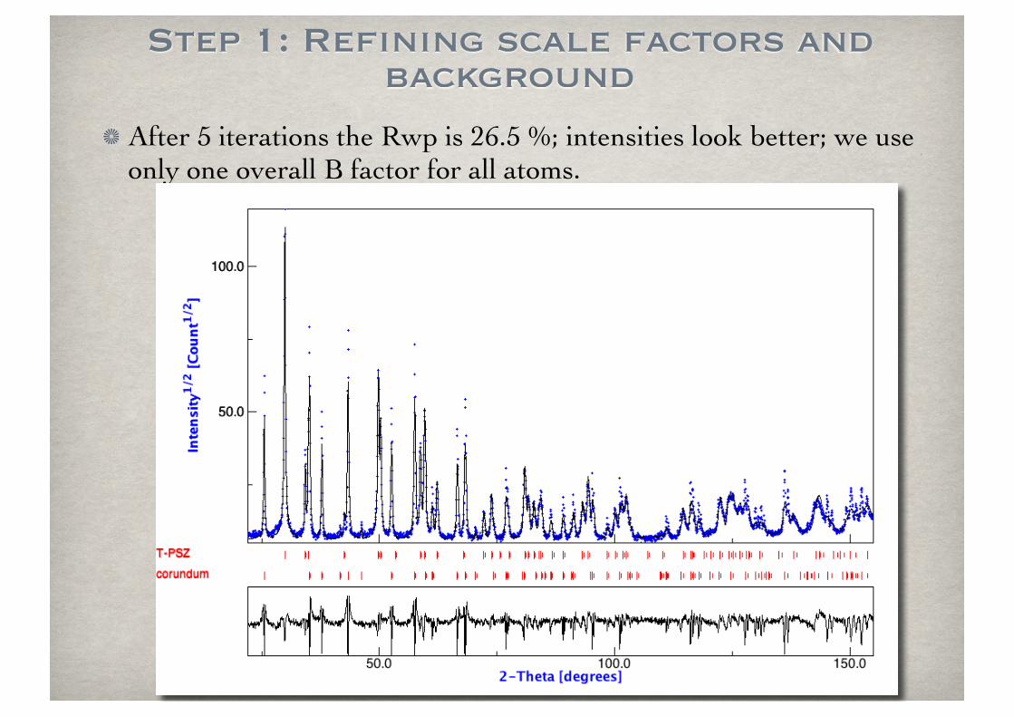
Step 1: Refining scale factors and background
After 5 iterations the Rwp is 26.5 %; intensities look better; we use only one overall B factor for all atoms.
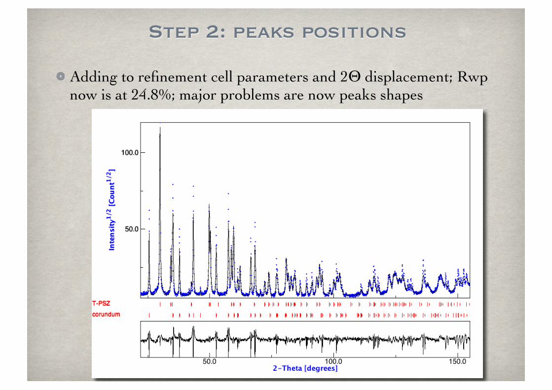
Step 2: peaks positions
Adding to refinement cell parameters and 2Θ displacement; Rwp now is at 24.8%; major problems are now peaks shapes
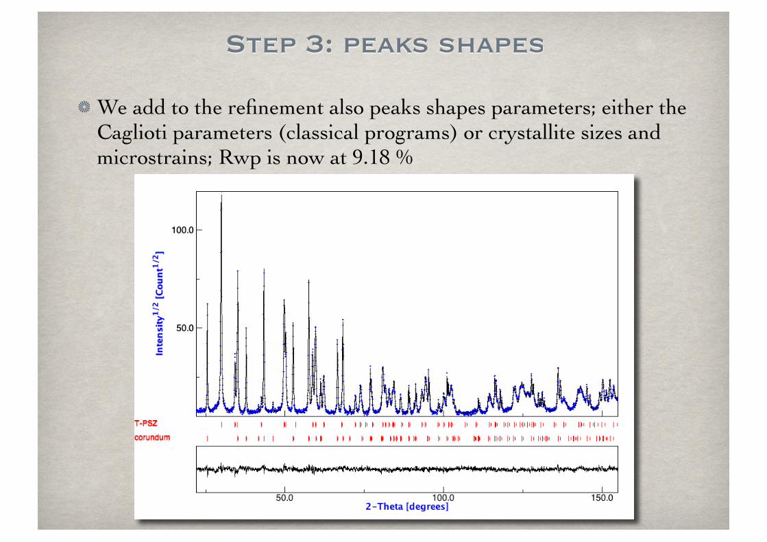
Step 3: peaks shapes
We add to the refinement also peaks shapes parameters; either the Caglioti parameters (classical programs) or crystallite sizes and microstrains; Rwp is now at 9.18 %
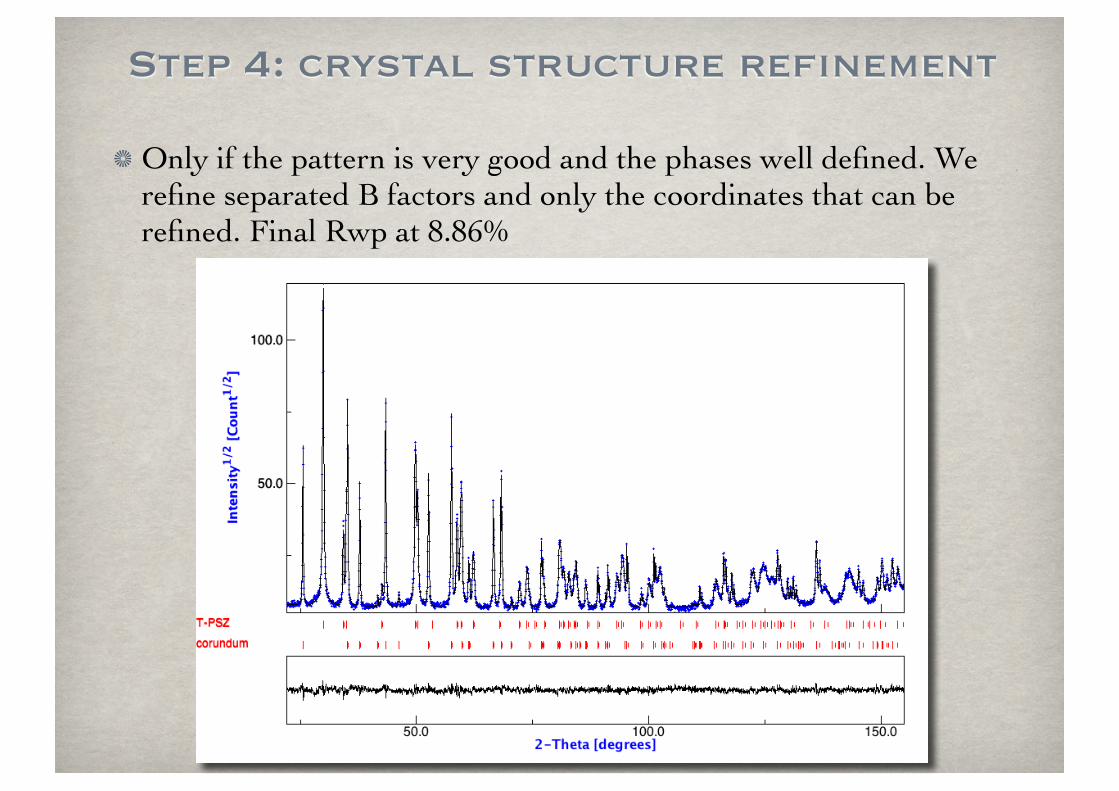
Step 4: crystal structure refinement
Only if the pattern is very good and the phases well defined. We refine separated B factors and only the coordinates that can be refined. Final Rwp at 8.86%
Quality of the experiment
A good diffraction fitting, a successful Rietveld analysis, they depend strongly on the quality of the experiment:
Instrument:
instrument characteristics and assessment
choice of instrument options
Collection strategies
range
step size
collection time
etc.
sample
sample size
sample preparation
sample condition
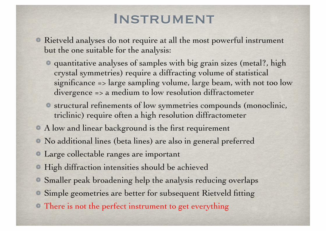
InstrumentRietveld analyses do not require at all the most powerful instrument but the one suitable for the analysis:
quantitative analyses of samples with big grain sizes (metal?, high crystal symmetries) require a diffracting volume of statistical significance => large sampling volume, large beam, with not too low divergence => a medium to low resolution diffractometer
structural refinements of low symmetries compounds (monoclinic, triclinic) require often a high resolution diffractometer
A low and linear background is the first requirement
No additional lines (beta lines) are also in general preferred
Large collectable ranges are important
High diffraction intensities should be achieved
Smaller peak broadening help the analysis reducing overlaps
Simple geometries are better for subsequent Rietveld fitting
There is not the perfect instrument to get everything
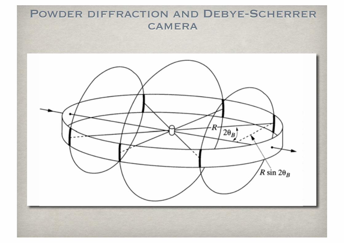
Powder diffraction and Debye-Scherrer camera
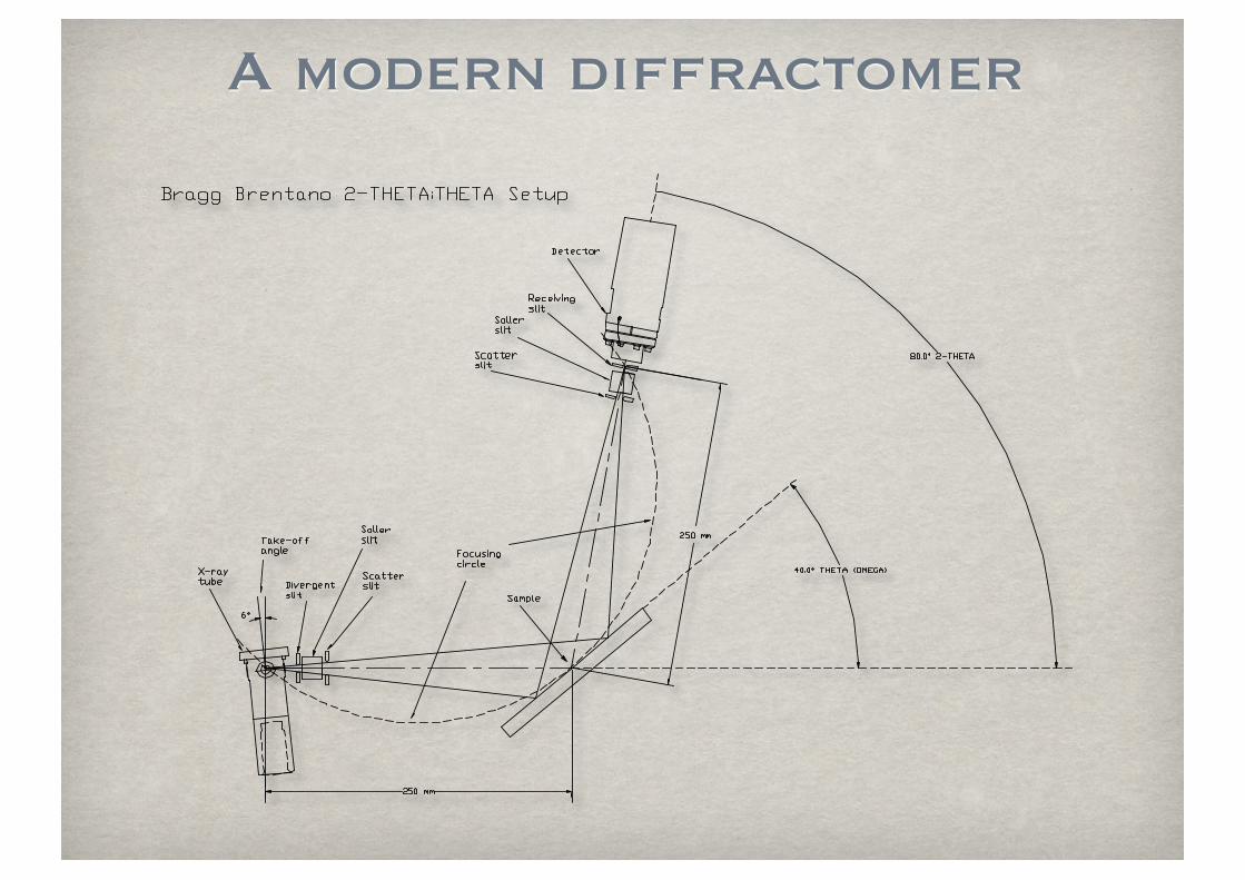
A modern diffractomer

Parafocusing circle (Bragg-Brentano)
Diffractometer
circle
Sample
Receiving slit
X-ray sourceFocusing circle
Incident beam
slit
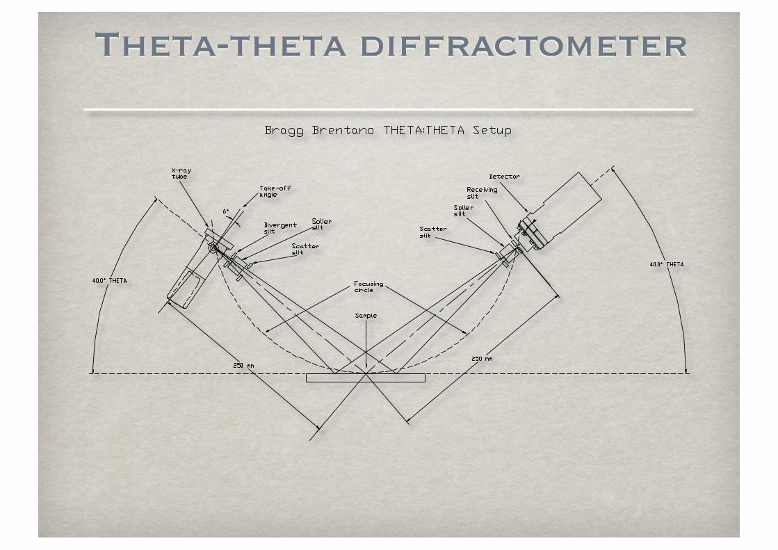
Theta-theta diffractometer
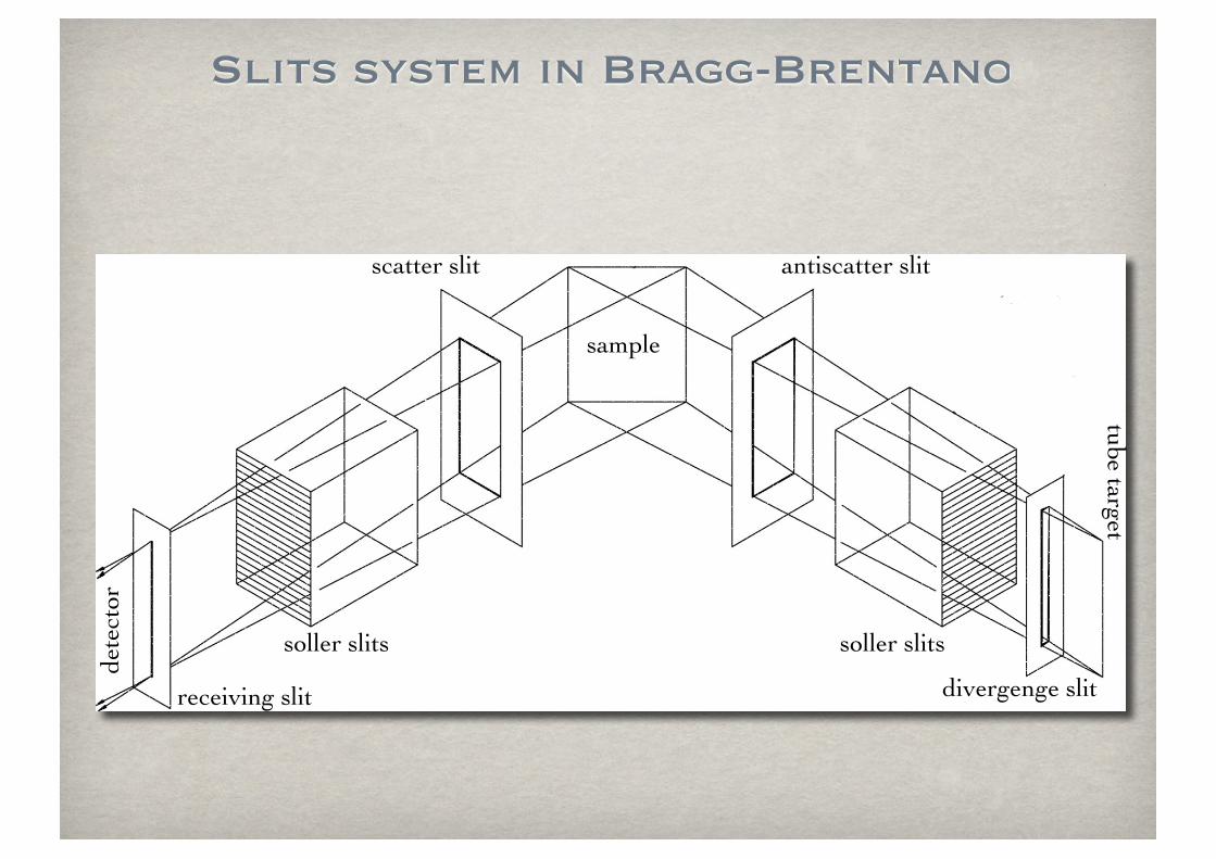
Slits system in Bragg-Brentano
soller slits
sample
divergenge slit
soller slits
receiving slit
antiscatter slitscatter slit
tube targetde
tect
or
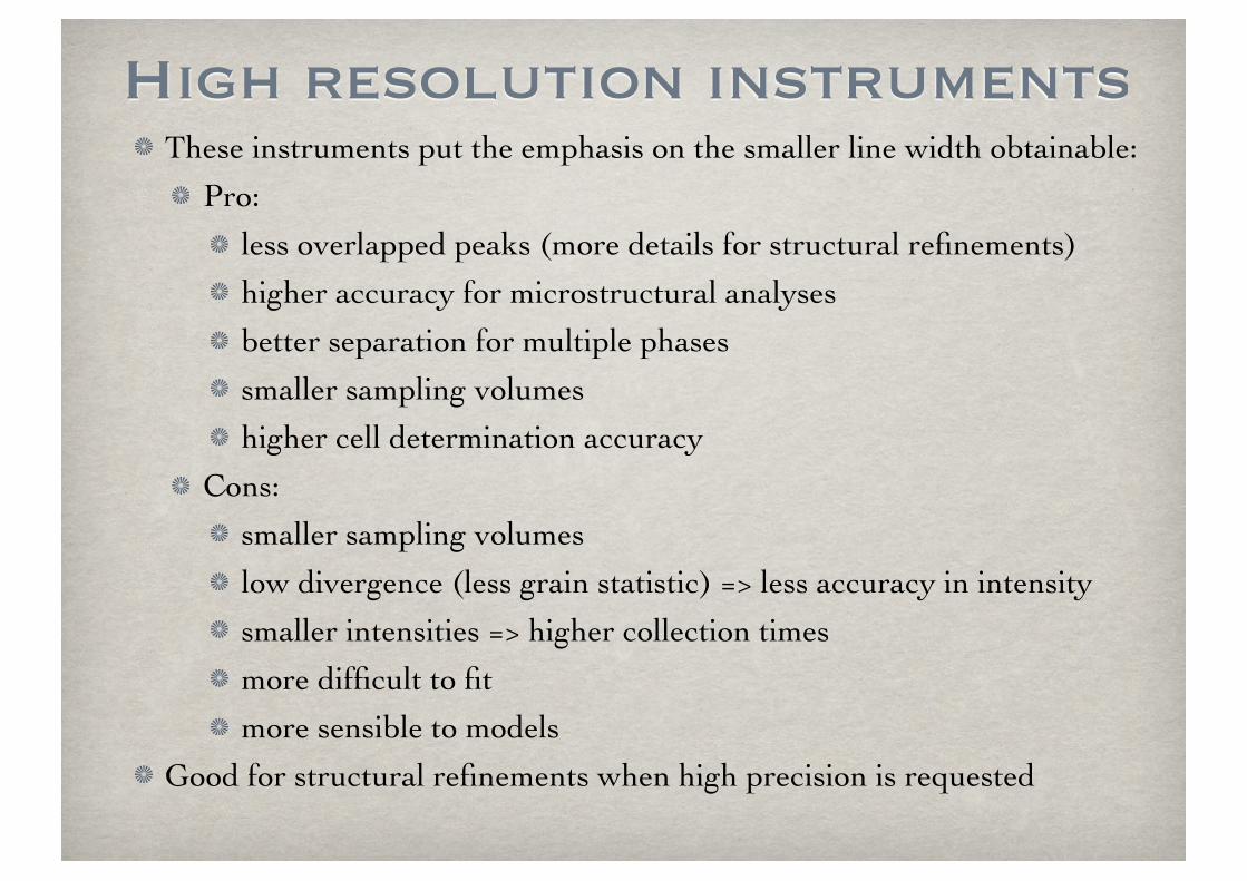
High resolution instrumentsThese instruments put the emphasis on the smaller line width obtainable:
Pro:
less overlapped peaks (more details for structural refinements)
higher accuracy for microstructural analyses
better separation for multiple phases
smaller sampling volumes
higher cell determination accuracy
Cons:
smaller sampling volumes
low divergence (less grain statistic) => less accuracy in intensity
smaller intensities => higher collection times
more difficult to fit
more sensible to models
Good for structural refinements when high precision is requested
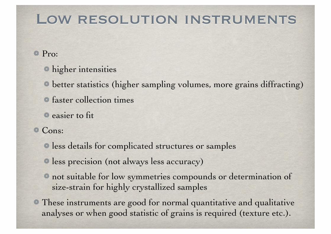
Low resolution instruments
Pro:
higher intensities
better statistics (higher sampling volumes, more grains diffracting)
faster collection times
easier to fit
Cons:
less details for complicated structures or samples
less precision (not always less accuracy)
not suitable for low symmetries compounds or determination of size-strain for highly crystallized samples
These instruments are good for normal quantitative and qualitative analyses or when good statistic of grains is required (texture etc.).
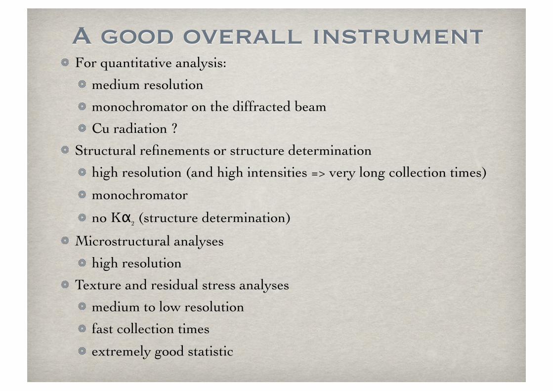
A good overall instrumentFor quantitative analysis:
medium resolution
monochromator on the diffracted beam
Cu radiation ?
Structural refinements or structure determination
high resolution (and high intensities => very long collection times)
monochromator
no Kα2 (structure determination)
Microstructural analyses
high resolution
Texture and residual stress analyses
medium to low resolution
fast collection times
extremely good statistic
Instrument assessment
In most cases (or always) the instrument alignment and setting is more important than the instrument itself
Be paranoid on alignment, the beam should pass through the unique rotation center and hits the detector at zero 2θ
The background should be linear, no strange bumps, no additional lines and as low as possible
Check the omega zero
Collect regularly a standard for line positions and check if the positions are good both at low and high diffraction angle (check also the rest)
The data collection
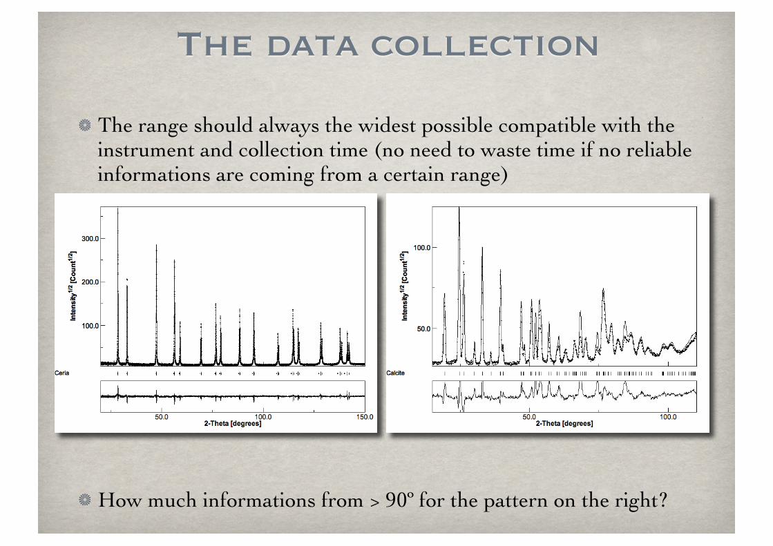
The range should always the widest possible compatible with the instrument and collection time (no need to waste time if no reliable informations are coming from a certain range)
How much informations from > 90º for the pattern on the right?

The step size
The step size should be compatible with the line broadening characteristics and type of analysis.
In general 5-7 points in the half upper part of a peak are sufficient to define its shape.
Slightly more points are preferred in case of severe overlapping.
A little more for size-strain analysis.
Too much points (too small step size) do not increase our resolution, accuracy or precision, but just increase the noise at equal total collection time.
The best solution is to use the higher step size possible that do not compromise the information we need.
Normally highly broadened peaks => big step size => less noise as we can increase the collection time per step (> 0.05)
very sharp peaks => small step size (from 0.02 to 0.05 for Bragg-Brentano)
Total collection time
Ensure the noise is lower than the intensity of small peaks.
If the total collection time is limited, better a lower noise than a smaller step size.
Better to collect a little bit more than to have to repeat an experiment.
If collection time is a problem go for line or 2D detectors:
CPS 120: 2 to 5 minutes for a good spectrum of 120 degrees (good for quantitative analyses or follow reactions, transformations, analyses in temperature)
Image plate or CCDs: very fast collection times when texture is needed or is a problem
Data quality (not related to intensity) of these detectors is a little bit lower than the one from good point detectors. But sometimes intensity rules!
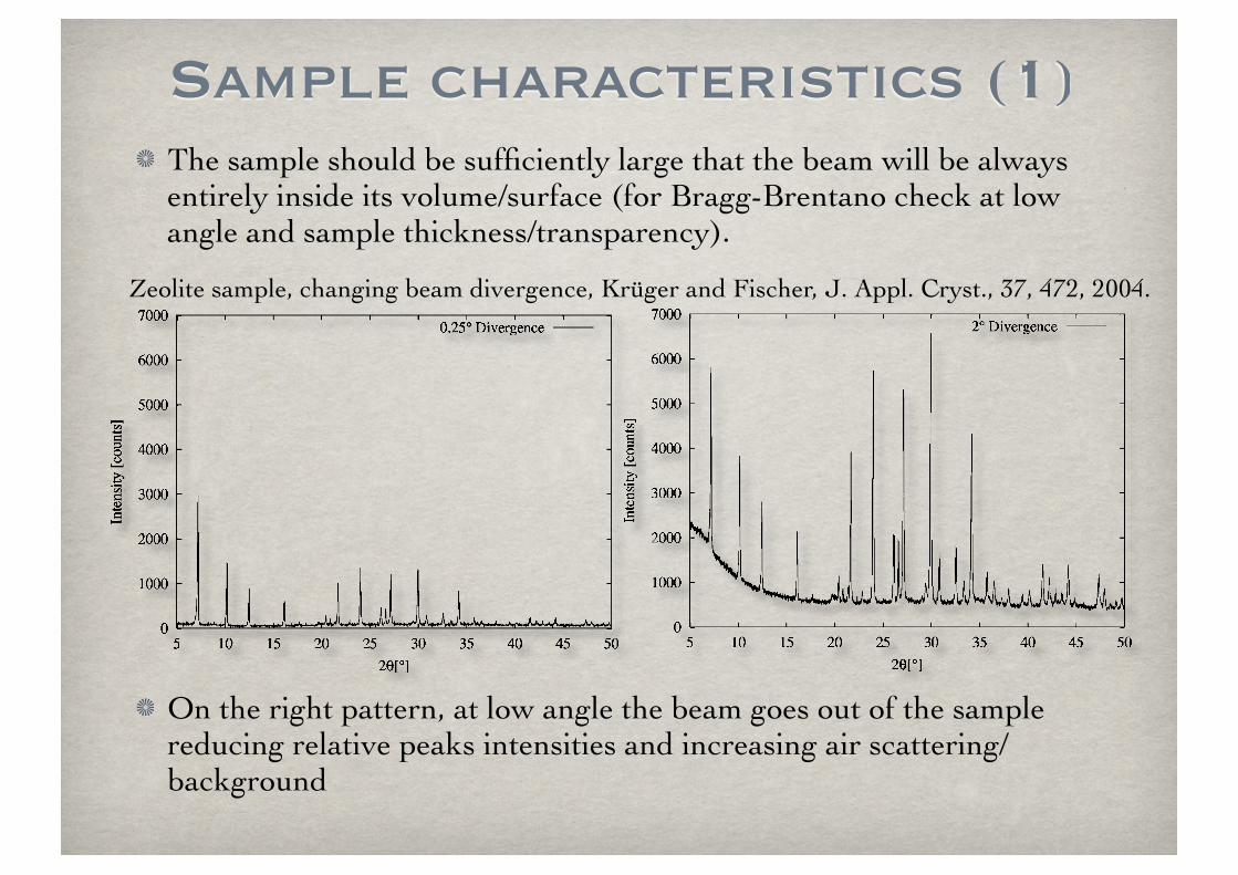
The sample should be sufficiently large that the beam will be always entirely inside its volume/surface (for Bragg-Brentano check at low angle and sample thickness/transparency).
On the right pattern, at low angle the beam goes out of the sample reducing relative peaks intensities and increasing air scattering/background
Zeolite sample, changing beam divergence, Krüger and Fischer, J. Appl. Cryst., 37, 472, 2004.
Sample characteristics (1)
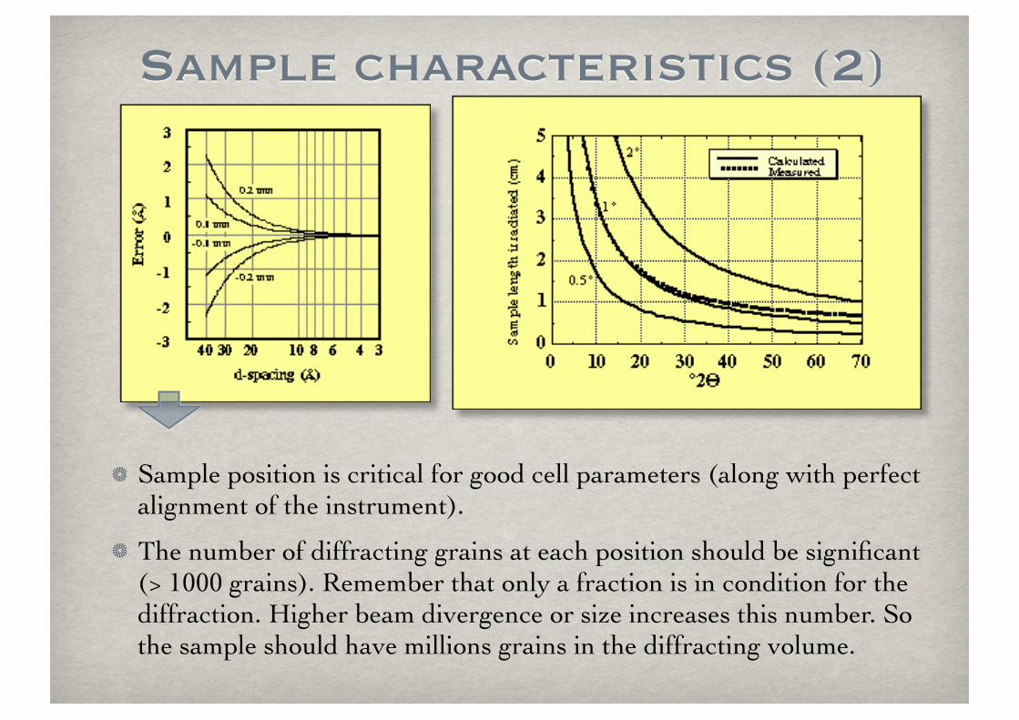
Sample characteristics (2)
Sample position is critical for good cell parameters (along with perfect alignment of the instrument).
The number of diffracting grains at each position should be significant (> 1000 grains). Remember that only a fraction is in condition for the diffraction. Higher beam divergence or size increases this number. So the sample should have millions grains in the diffracting volume.
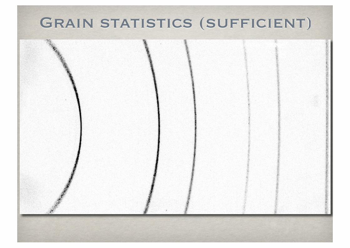
Grain statistics (sufficient)
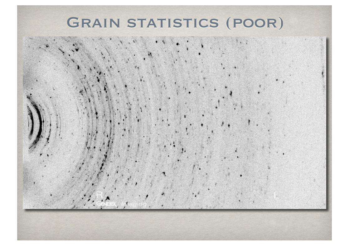
Grain statistics (poor)
Sample characteristics
The sample should be sufficiently large that the beam will be entirely inside its volume/surface (always)
Sample position is critical for good cell parameters (along with perfect alignment of the instrument)
The number of diffracting grains at each position should be significant (> 1000 grains). Remember that only a fraction is in condition for the diffraction. Higher beam divergence or size increases this number.
Unless a texture analysis is the goal, no preferred orientations should be present. Change sample preparation if necessary.
The sample should be homogeneous.
Be aware of absorption contrast problems
In Bragg-Brentano geometry the thickness should be infinite respect to the absorption.
Quality of the surface matters.
Ambient conditions
In some cases constant ambient condition are important:
temperature for cell parameter determination or phase transitions
humidity for some organic compounds or pharmaceuticals
can your sample be damaged or modify by irradiation (normally Copper or not too highly energetic radiations are not)
There are special attachments to control the ambient for sensitive compounds
Non classical Rietveld applications
Along with the refinement of crystal structures the concept of the Rietveld method has been extended to other diffraction analyses. Most of them more useful for people working on material science. These are:
Quantitative phase analyses
Amorphous quantification
Microstructural analyses
Texture and Residual stresses
Expert tricks/suggestion
First get a good experiment/spectrum
Know your sample as much as possible
Do not refine too many parameters
Always try first to manually fit the spectrum as much as possible
Never stop at the first result
Look carefully and constantly to the visual fit/plot and residuals during refinement process (no “blind” refinement)
Zoom in the plot and look at the residuals. Try to understand what is causing a bad fit.
Do not plot absolute intensities; plot at iso-statistical errors. Small peaks are important like big peaks.
Use all the indices and check parameter errors.
First get a good experiment/spectrum


