62
PART ONE Introduction to Discrete-Event System Simulation
PART ONE
Introduction to
Discrete-Event System
Simulation

1Introduction to Simulation
A simulation is the imitation of the operation of a real-world process or sys-tem over time. Whether done by hand or on a computer, simulation involvesthe generation of an artificial history of a system, and the observation of thatartificial history to draw inferences concerning the operating characteristics ofthe real system.
The behavior of a system as it evolves over time is studied by developinga simulation model. This model usually takes the form of a set of assumptionsconcerning the operation of the system. These assumptions are expressed inmathematical, logical, and symbolic relationships between the entities, or ob-jects of interest, of the system. Once developed and validated, a model canbe used to investigate a wide variety of “what-if” questions about the real-world system. Potential changes to the system can first be simulated in orderto predict their impact on system performance. Simulation can also be used tostudy systems in the design stage, before such systems are built. Thus, simula-tion modeling can be used both as an analysis tool for predicting the effect ofchanges to existing systems, and as a design tool to predict the performance ofnew systems under varying sets of circumstances.
In some instances, a model can be developed which is simple enough tobe “solved” by mathematical methods. Such solutions may be found by the useof differential calculus, probability theory, algebraic methods, or other math-ematical techniques. The solution usually consists of one or more numericalparameters which are called measures of performance of the system. How-ever, many real-world systems are so complex that models of these systemsare virtually impossible to solve mathematically. In these instances, numerical,computer-based simulation can be used to imitate the behavior of the system
3
4 Chap. 1 Introduction to Simulation
over time. From the simulation, data are collected as if a real system were beingobserved. This simulation-generated data is used to estimate the measures ofperformance of the system.
This book provides an introductory treatment of the concepts and meth-ods of one form of simulation modeling—discrete-event simulation modeling.The first chapter initially discusses when to use simulation, its advantages anddisadvantages, and actual areas of application. Then the concepts of systemand model are explored. Finally, an outline is given of the steps in building andusing a simulation model of a system.
1.1 When Is Simulation the Appropriate Tool?
The availability of special-purpose simulation languages, massive computingcapabilities at a decreasing cost per operation, and advances in simulationmethodologies have made simulation one of the most widely used and acceptedtools in operations research and systems analysis. Circumstances under whichsimulation is the appropriate tool to use have been discussed by many authors,from Naylor et al. [1966] to Banks et al. [1996]. Simulation can be used for thefollowing purposes:
1. Simulation enables the study of, and experimentation with, the internalinteractions of a complex system, or of a subsystem within a complexsystem.
2. Informational, organizational, and environmental changes can be simu-lated, and the effect of these alterations on the model’s behavior can beobserved.
3. The knowledge gained in designing a simulation model may be of greatvalue toward suggesting improvement in the system under investigation.
4. By changing simulation inputs and observing the resulting outputs, valu-able insight may be obtained into which variables are most important andhow variables interact.
5. Simulation can be used as a pedagogical device to reinforce analytic so-lution methodologies.
6. Simulation can be used to experiment with new designs or policies priorto implementation, so as to prepare for what may happen.
7. Simulation can be used to verify analytic solutions.
8. By simulating different capabilities for a machine, requirements can bedetermined.
9. Simulation models designed for training allow learning without the costand disruption of on-the-job learning.
Sec. 1.2 When Simulation Is Not Appropriate 5
10. Animation shows a system in simulated operation so that the plan can bevisualized.
11. The modern system (factory, wafer fabrication plant, service organization,etc.) is so complex that the interactions can be treated only throughsimulation.
1.2 When Simulation Is Not Appropriate
This section is based on an article by Banks and Gibson [1997], who gaveten rules for determining when simulation is not appropriate. The first ruleindicates that simulation should not be used when the problem can be solvedusing common sense. An example is given of an automobile-tag facility servingcustomers who arrive randomly at an average rate of 100/hour and are served ata mean rate of 12/hour. To determine the minimum number of servers needed,simulation is not necessary. Just compute 100/12 = 8.33, indicating that nine ormore servers are needed.
The second rule says that simulation should not be used if the problemcan be solved analytically. For example, under certain conditions, the averagewaiting time in the example above can be determined from curves that weredeveloped by Hillier and Lieberman [1995].
The next rule says that simulation should not be used if it is easier toperform direct experiments. An example of a fast-food drive-in restaurant isgiven, where it was less expensive to have a person use a hand-held terminal andvoice communication to determine the effect of adding another order stationon customer waiting time.
The fourth rule says not to use simulation, if the costs exceed the savings.There are many steps in completing a simulation as discussed in Section 1.11,and these must be done thoroughly. If a simulation study costs $20,000 and thesavings might be $10,000, simulation would not be appropriate.
Rules five and six indicate that simulation should not be performed if theresources or time are not available. If the simulation is estimated to cost $20,000and only $10,000 is available, the suggestion is not to venture into a simulationstudy. Similarly, if a decision in needed is two weeks and a simulation will takea month, the simulation study is not advised.
Simulation takes data, sometimes lots of data. If no data is available, noteven estimates, simulation is not advised.
The next rule concerns the ability to verify and validate the model. Ifthere is not enough time or the personnel are not available, simulation is notappropriate.
If managers have unreasonable expectations—say, too much too soon—or the power of simulation is overestimated, simulation may not be appropriate.
Last, if system behavior is too complex or can’t be defined, simulation isnot appropriate. Human behavior is sometimes extremely complex to model.

6 Chap. 1 Introduction to Simulation
1.3 Advantages and Disadvantages of Simulation
Simulation is intuitively appealing to a client because it mimics what happensin a real system or what is perceived for a system that is in the design stage. Theoutput data from a simulation should directly correspond to the outputs thatcould be recorded from the real system. Additionally, it is possible to developa simulation model of a system without dubious assumptions (such as the samestatistical distribution for every random variable) of mathematically solvablemodels. For these, and other reasons, simulation is frequently the technique ofchoice in problem solving.
In contrast to optimization models, simulation models are “run” ratherthan solved. Given a particular set of input and model characteristics, the modelis run and the simulated behavior is observed. This process of changing inputsand model characteristics results in a set of scenarios that are evaluated. Agood solution, either in the analysis of an existing system or the design of a newsystem, is then recommended for implementation.
Simulation has many advantages, and even some disadvantages. Theseare listed by Pegden, Shannon, and Sadowski [1995]. The advantages are:
1. New policies, operating procedures, decision rules, information flows, or-ganizational procedures, and so on can be explored without disruptingongoing operations of the real system.
2. New hardware designs, physical layouts, transportation systems, and soon, can be tested without committing resources for their acquisition.
3. Hypotheses about how or why certain phenomena occur can be testedfor feasibility.
4. Time can be compressed or expanded allowing for a speedup or slowdownof the phenomena under investigation.
5. Insight can be obtained about the interaction of variables.
6. Insight can be obtained about the importance of variables to the perfor-mance of the system.
7. Bottleneck analysis can be performed indicating where work-in-process,information, materials, and so on are being excessively delayed.
8. A simulation study can help in understanding how the system operatesrather than how individuals think the system operates.
9. “What-if” questions can be answered. This is particularly useful in thedesign of new systems.
The disadvantages are:
1. Model building requires special training. It is an art that is learned overtime and through experience. Furthermore, if two models are constructedby two competent individuals, they may have similarities, but it is highlyunlikely that they will be the same.

Sec. 1.4 Areas of Application 7
2. Simulation results may be difficult to interpret. Since most simulationoutputs are essentially random variables (they are usually based on ran-dom inputs), it may be hard to determine whether an observation is aresult of system interrelationships or randomness.
3. Simulation modeling and analysis can be time consuming and expensive.Skimping on resources for modeling and analysis may result in a simula-tion model or analysis that is not sufficient for the task.
4. Simulation is used in some cases when an analytical solution is possible,or even preferable, as discussed in Section 1.2. This might be particularlytrue in the simulation of some waiting lines where closed-form queueingmodels are available.
In defense of simulation, these four disadvantages, respectively, can be offsetas follows:
1. Vendors of simulation software have been actively developing packagesthat contain models that need only input data for their operation. Suchmodels have the generic tag “simulators” or “templates.”
2. Many simulation software vendors have developed output analysis capa-bilities within their packages for performing very thorough analysis.
3. Simulation can be performed faster today than yesterday, and even fastertomorrow. This is attributable to the advances in hardware that permitrapid running of scenarios. It is also attributable to the advances in manysimulation packages. For example, some simulation software containsconstructs for modeling material handling using transporters such as forklift trucks, conveyors, automated guided vehicles, and others.
4. Closed-form models are not able to analyze most of the complex systemsthat are encountered in practice. In nearly eight years of consulting prac-tice by one of the authors, not one problem was encountered that couldhave been solved by a closed-form solution.
1.4 Areas of Application
The applications of simulation are vast. The Winter Simulation Conference(WSC) is an excellent way to learn more about the latest in simulation ap-plications and theory. There are also numerous tutorials at both the begin-ning and advanced levels. WSC is sponsored by six technical societies and theNational Institute of Standards and Technology (NIST). The technical soci-eties are American Statistical Association (ASA), Association for ComputingMachinery/Special Interest Group on Simulation (ACM/SIGSIM), Instituteof Electrical and Electronics Engineers: Computer Society (IEEE/CS), Insti-tute of Electrical and Electronics Engineers: Systems, Man and CyberneticsSociety (IEEE/SMCS), Institute of Industrial Engineers (IIE), Institute forOperations Research and the Management Sciences: College on Simulation(INFORMS/CS), and The Society for Computer Simulation (SCS). Note that

8 Chap. 1 Introduction to Simulation
IEEE is represented by two bodies. Information about the upcoming WSC canbe obtained from
www.wintersim.org
Some of the areas of application at a recent WSC, with the subject matterwithin those areas, is listed below:
Manufacturing Applications
Analysis of electronics assembly operationsDesign and evaluation of a selective assembly station for high-precision
scroll compressor shellsComparison of dispatching rules for semiconductor manufacturing using
large-facility modelsEvaluation of cluster tool throughput for thin-film head productionDetermining optimal lot size for a semiconductor back-end factoryOptimization of cycle time and utilization in semiconductor test manufac-
turingAnalysis of storage and retrieval strategies in a warehouseInvestigation of dynamics in a service-oriented supply chainModel for an Army chemical munitions disposal facility
Semiconductor Manufacturing
Comparison of dispatching rules using large-facility modelsThe corrupting influence of variabilityA new lot-release rule for wafer fabsAssessment of potential gains in productivity due to proactive reticle man-
agementComparison of a 200-mm and 300-mm X-ray lithography cellCapacity planning with time constraints between operations300-mm logistic system risk reduction
Construction Engineering
Construction of a dam embankmentTrenchless renewal of underground urban infrastructuresActivity scheduling in a dynamic, multiproject settingInvestigation of the structural steel erection processSpecial-purpose template for utility tunnel construction

Sec. 1.5 Systems and System Environment 9
Military ApplicationsModeling leadership effects and recruit type in an Army recruiting stationDesign and test of an intelligent controller for autonomous underwater ve-
hiclesModeling military requirements for nonwarfighting operationsMultitrajectory performance for varying scenario sizesUsing adaptive agents in U.S. Air Force pilot retention
Logistics, Transportation, and Distribution ApplicationsEvaluating the potential benefits of a rail-traffic planning algorithmEvaluating strategies to improve railroad performanceParametric modeling in rail-capacity planningAnalysis of passenger flows in an airport terminalProactive flight-schedule evaluationLogistics issues in autonomous food production systems for extended-duration
space explorationSizing industrial rail-car fleetsProduct distribution in the newspaper industryDesign of a toll plazaChoosing between rental-car locationsQuick-response replenishment
Business Process SimulationImpact of connection bank redesign on airport gate assignmentProduct development program planningReconciliation of business and systems modelingPersonnel forecasting and strategic workforce planning
Human SystemsModeling human performance in complex systemsStudying the human element in air traffic control
1.5 Systems and System Environment
To model a system, it is necessary to understand the concept of a system andthe system boundary. A system is defined as a group of objects that are joinedtogether in some regular interaction or interdependence toward the accom-plishment of some purpose. An example is a production system manufacturingautomobiles. The machines, component parts, and workers operate jointlyalong an assembly line to produce a high-quality vehicle.
A system is often affected by changes occurring outside the system. Suchchanges are said to occur in the system environment [Gordon, 1978]. In model-ing systems, it is necessary to decide on the boundary between the system andits environment. This decision may depend on the purpose of the study.

10 Chap. 1 Introduction to Simulation
In the case of the factory system, for example, the factors controlling thearrival of orders may be considered to be outside the influence of the factoryand therefore part of the environment. However, if the effect of supply ondemand is to be considered, there will be a relationship between factoryoutput and arrival of orders, and this relationship must be considered anactivity of the system. Similarly, in the case of a bank system, there may be alimit on the maximum interest rate that can be paid. For the study of a singlebank, this would be regarded as a constraint imposed by the environment.In a study of the effects of monetary laws on the banking industry, however,the setting of the limit would be an activity of the system. [Gordon, 1978]
1.6 Components of a System
In order to understand and analyze a system, a number of terms need to bedefined. An entity is an object of interest in the system. An attribute is aproperty of an entity. An activity represents a time period of specified length.If a bank is being studied, customers might be one of the entities, the balancein their checking accounts might be an attribute, and making deposits might bean activity.
The collection of entities that compose a system for one study mightbe only a subset of the overall system for another study [Law and Kelton,2000]. For example, if the bank mentioned above is being studied to determinethe number of tellers needed to provide for paying and receiving, the systemcan be defined as that portion of the bank consisting of the regular tellersand the customers waiting in line. If the purpose of the study is expanded todetermine the number of special tellers needed (to prepare cashier’s checks, tosell traveler’s checks, etc.), the definition of the system must be expanded.
The state of a system is defined to be that collection of variables necessaryto describe the system at any time, relative to the objectives of the study. Inthe study of a bank, possible state variables are the number of busy tellers, thenumber of customers waiting in line or being served, and the arrival time ofthe next customer. An event is defined as an instantaneous occurrence thatmay change the state of the system. The term endogenous is used to describeactivities and events occurring within a system, and the term exogenous is usedto describe activities and events in the environment that affect the system.In the bank study, the arrival of a customer is an exogenous event, and thecompletion of service of a customer is an endogenous event.
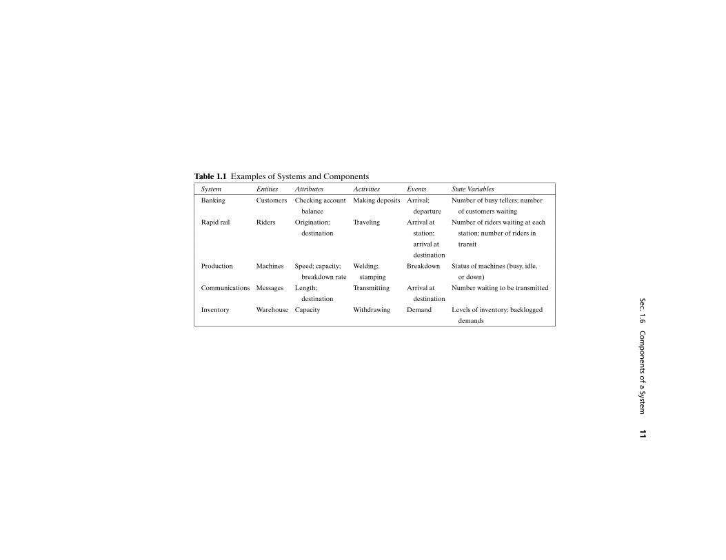
Table 1.1 lists examples of entities, attributes, activities, events, and statevariables for several systems. Only a partial listing of the system componentsis shown. A complete list cannot be developed unless the purpose of the studyis known. Depending on the purpose, various aspects of the system will be ofinterest, and then the listing of components can be completed.
Sec.1.6C
om
po
nen
tso
fa
System11
Table 1.1 Examples of Systems and Components
System Entities Attributes Activities Events State Variables
Banking Customers Checking account Making deposits Arrival; Number of busy tellers; number
balance departure of customers waiting
Rapid rail Riders Origination; Traveling Arrival at Number of riders waiting at each
destination station; station; number of riders in
arrival at transit
destination
Production Machines Speed; capacity; Welding; Breakdown Status of machines (busy, idle,
breakdown rate stamping or down)
Communications Messages Length; Transmitting Arrival at Number waiting to be transmitted
destination destination
Inventory Warehouse Capacity Withdrawing Demand Levels of inventory; backlogged
demands
12 Chap. 1 Introduction to Simulation
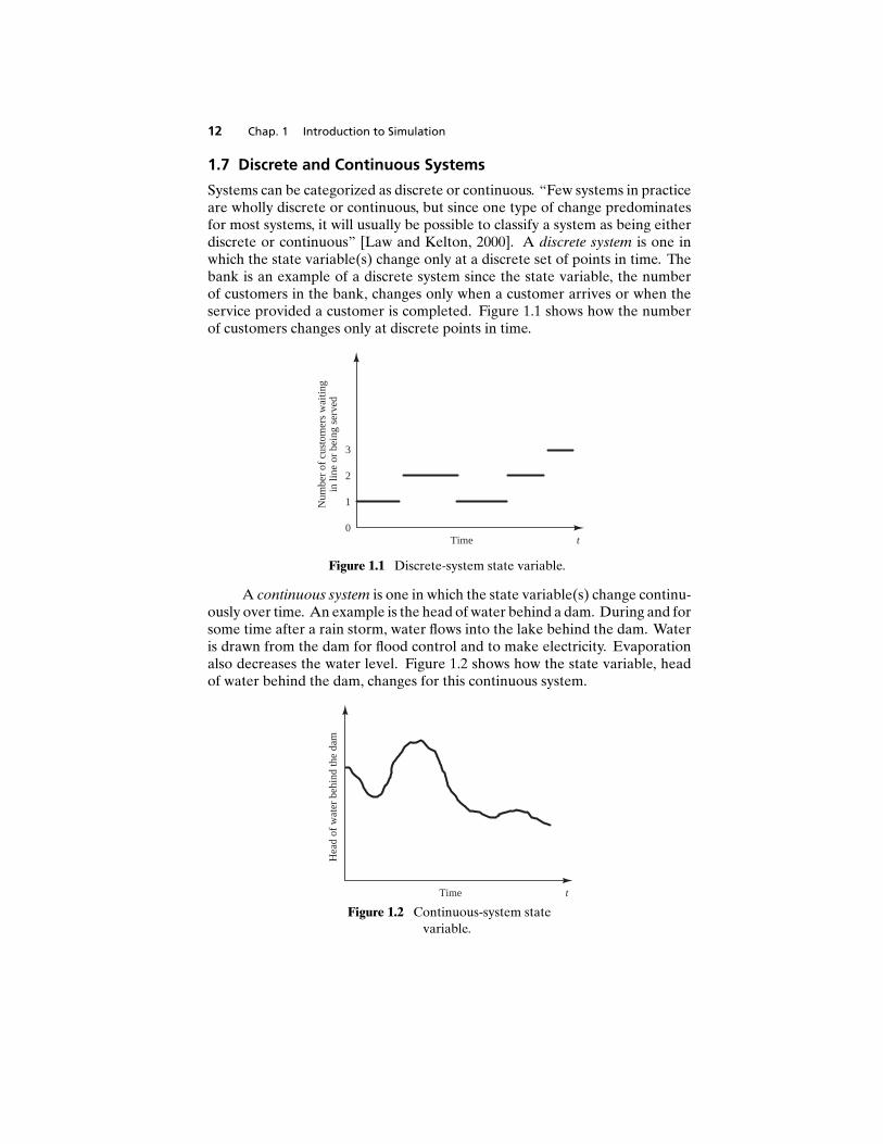
1.7 Discrete and Continuous Systems
Systems can be categorized as discrete or continuous. “Few systems in practiceare wholly discrete or continuous, but since one type of change predominatesfor most systems, it will usually be possible to classify a system as being eitherdiscrete or continuous” [Law and Kelton, 2000]. A discrete system is one inwhich the state variable(s) change only at a discrete set of points in time. Thebank is an example of a discrete system since the state variable, the numberof customers in the bank, changes only when a customer arrives or when theservice provided a customer is completed. Figure 1.1 shows how the numberof customers changes only at discrete points in time.
Time t0
1
2
3
Num
ber
of c
usto
mer
s w
aitin
gin
line
or
bein
g se
rved
Figure 1.1 Discrete-system state variable.
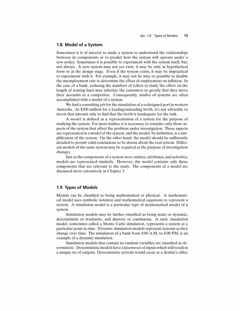
A continuous system is one in which the state variable(s) change continu-ously over time. An example is the head of water behind a dam. During and forsome time after a rain storm, water flows into the lake behind the dam. Wateris drawn from the dam for flood control and to make electricity. Evaporationalso decreases the water level. Figure 1.2 shows how the state variable, headof water behind the dam, changes for this continuous system.
Time t
Hea
d of
wat
er b
ehin
d th
e da
m
Figure 1.2 Continuous-system statevariable.
Sec. 1.9 Types of Models 13
1.8 Model of a System
Sometimes it is of interest to study a system to understand the relationshipsbetween its components or to predict how the system will operate under anew policy. Sometimes it is possible to experiment with the system itself, but,not always. A new system may not yet exist; it may be only in hypotheticalform or at the design stage. Even if the system exists, it may be impracticalto experiment with it. For example, it may not be wise or possible to doublethe unemployment rate to determine the effect of employment on inflation. Inthe case of a bank, reducing the numbers of tellers to study the effect on thelength of waiting lines may infuriate the customers so greatly that they movetheir accounts to a competitor. Consequently, studies of systems are oftenaccomplished with a model of a system.
We had a consulting job for the simulation of a redesigned port in westernAustralia. At $200 million for a loading/unloading berth, it’s not advisable toinvest that amount only to find that the berth is inadequate for the task.
A model is defined as a representation of a system for the purpose ofstudying the system. For most studies, it is necessary to consider only those as-pects of the system that affect the problem under investigation. These aspectsare represented in a model of the system, and the model, by definition, is a sim-plification of the system. On the other hand, the model should be sufficientlydetailed to permit valid conclusions to be drawn about the real system. Differ-ent models of the same system may be required as the purpose of investigationchanges.
Just as the components of a system were entities, attributes, and activities,models are represented similarly. However, the model contains only thosecomponents that are relevant to the study. The components of a model arediscussed more extensively in Chapter 3.
1.9 Types of Models
Models can be classified as being mathematical or physical. A mathemati-cal model uses symbolic notation and mathematical equations to represent asystem. A simulation model is a particular type of mathematical model of asystem.
Simulation models may be further classified as being static or dynamic,deterministic or stochastic, and discrete or continuous. A static simulationmodel, sometimes called a Monte Carlo simulation, represents a system at aparticular point in time. Dynamic simulation models represent systems as theychange over time. The simulation of a bank from 9:00 A.M. to 4:00 P.M. is anexample of a dynamic simulation.
Simulation models that contain no random variables are classified as de-terministic. Deterministic models have a known set of inputs which will result ina unique set of outputs. Deterministic arrivals would occur at a dentist’s office
14 Chap. 1 Introduction to Simulation
if all patients arrived at the scheduled appointment time. A stochastic simula-tion model has one or more random variables as inputs. Random inputs lead torandom outputs. Since the outputs are random, they can be considered only asestimates of the true characteristics of a model. The simulation of a bank wouldusually involve random interarrival times and random service times. Thus, ina stochastic simulation, the output measures—the average number of peoplewaiting, the average waiting time of a customer—must be treated as statisticalestimates of the true characteristics of the system.
Discrete and continuous systems were defined in Section 1.6. Discreteand continuous models are defined in an analogous manner. However, a dis-crete simulation model is not always used to model a discrete system, nor is acontinuous simulation model always used to model a continuous system. Tanksand pipes are modeled discretely by some software vendors, even though weknow that fluid flow is continuous. In addition, simulation models may bemixed, both discrete and continuous. The choice of whether to use a discreteor continuous (or both discrete and continuous) simulation model is a func-tion of the characteristics of the system and the objective of the study. Thus, acommunication channel could be modeled discretely if the characteristics andmovement of each message were deemed important. Conversely, if the flowof messages in aggregate over the channel were of importance, modeling thesystem using continuous simulation could be more appropriate. The modelsconsidered in this text are discrete, dynamic, and stochastic.
1.10 Discrete-Event System Simulation
This book is about discrete-event system simulation—the modeling of systemsin which the state variable changes only at a discrete set of points in time.The simulation models are analyzed by numerical rather than by analyticalmethods. Analytical methods employ the deductive reasoning of mathemat-ics to “solve” the model. For example, differential calculus can be used todetermine the minimum-cost policy for some inventory models. Numericalmethods employ computational procedures to “solve” mathematical models.In the case of simulation models, which employ numerical methods, modelsare “run” rather than solved; that is, an artificial history of the system is gen-erated based on the model assumptions, and observations are collected to beanalyzed and to estimate the true system performance measures. Since real-world simulation models are rather large, and since the amount of data storedand manipulated is so vast, the runs are usually conducted with the aid of acomputer. However, much insight can be obtained by simulating small modelsmanually.
In summary, this book is about discrete-event system simulation in whichthe models of interest are analyzed numerically, usually with the aid of a com-puter.
Sec. 1.11 Steps in a Simulation Study 15
1.11 Steps in a Simulation Study
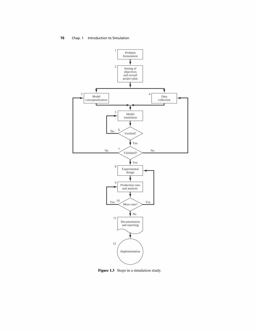
Figure 1.3 shows a set of steps to guide a model builder in a thorough and soundsimulation study. Similar figures and discussion of steps can be found in othersources [Shannon, 1975; Gordon, 1978; Law and Kelton, 2000]. The numberbeside each symbol in Figure 1.3 refers to the more detailed discussion in thetext. The steps in a simulation study are as follows:
Problem formulation. Every study should begin with a statement of the prob-lem. If the statement is provided by the policy makers, or those that have theproblem, the analyst must ensure that the problem being described is clearlyunderstood. If a problem statement is being developed by the analyst, it isimportant that the policy makers understand and agree with the formulation.Although not shown in Figure 1.3, there are occasions where the problem mustbe reformulated as the study progresses. In many instances, policy makers andanalysts are aware that there is a problem long before the nature of the problemis known.
Setting of objectives and overall project plan. The objectives indicate thequestions to be answered by simulation. At this point a determination shouldbe made concerning whether simulation is the appropriate methodology for theproblem as formulated and objectives as stated. Assuming it is decided thatsimulation is appropriate, the overall project plan should include a statementof the alternative systems to be considered, and a method for evaluating theeffectiveness of these alternatives. It should also include the plans for thestudy in terms of the number of people involved, the cost of the study, andthe number of days required to accomplish each phase of the work with theanticipated results at the end of each stage.
Model conceptualization. The construction of a model of a system is proba-bly as much art as science. Pritsker [1998] provides a lengthy discussion of thisstep. “Although it is not possible to provide a set of instructions that will leadto building successful and appropriate models in every instance, there are somegeneral guidelines that can be followed” [Morris, 1967]. The art of modeling isenhanced by an ability to abstract the essential features of a problem, to selectand modify basic assumptions that characterize the system, and then to enrichand elaborate the model until a useful approximation results. Thus, it is best tostart with a simple model and build toward greater complexity. However, themodel complexity need not exceed that required to accomplish the purposesfor which the model is intended. Violation of this principle will only add tomodel-building and computer expenses. It is not necessary to have a one-to-one mapping between the model and the real system. Only the essence of thereal system is needed.
It is advisable to involve the model user in model conceptualization. Thiswill both enhance the quality of the resulting model and increase the confidenceof the model user in the application of the model. (Chapter 2 describes a
16 Chap. 1 Introduction to Simulation
Problemformulation
Setting ofobjectivesand overallproject plan
1
2
Modelconceptualization
3Data
collection
4
5
6No
7No
Yes
Yes
No
Experimentaldesign
8
Production runsand analysis
9
10Yes
No
Yes
Documentationand reporting
11
12
Implementation
Verified?
Validated?
More runs?
Modeltranslation
Figure 1.3 Steps in a simulation study.

Sec. 1.11 Steps in a Simulation Study 17
number of simulation models. Chapter 6 describes queueing models that canbe solved analytically. However, only experience with real systems—versustextbook problems—can “teach” the art of model building.)
Data collection. There is a constant interplay between the construction ofthe model and the collection of the needed input data [Shannon, 1975]. As thecomplexity of the model changes, the required data elements may also change.Also, since data collection takes such a large portion of the total time requiredto perform a simulation, it is necessary to begin it as early as possible, usuallytogether with the early stages of model building.
The objectives of the study dictate, in a large way, the kind of data to becollected. In the study of a bank, for example, if the desire is to learn about thelength of waiting lines as the number of tellers change, the types of data neededwould be the distributions of interarrival times (at different times of the day),the service-time distributions for the tellers, and historic distributions on thelengths of waiting lines under varying conditions. These last data will be usedto validate the simulation model. (Chapter 9 discusses data collection and dataanalysis; Chapter 5 discusses statistical distributions which occur frequently insimulation modeling. See also an excellent discussion by Vincent [1998].)
Model translation. Since most real-world systems result in models that re-quire a great deal of information storage and computation, the model mustbe entered into a computer-recognizable format. We use the term “program,”even though it is possible to accomplish the desired result in many instanceswith little or no actual coding. The modeler must decide whether to programthe model in a simulation language such as GPSS/H© (discussed in Chapter 4)or to use special-purpose simulation software. For manufacturing and materialhandling, Chapter 4 discusses Arena®, AutoMod©, CSIM, Extend©, MicroSaint, ProModel®, Dened/Quest®, Taylor Eneterprise Dynamics (ED), andWitness©. Simulation languages are powerful and flexible. However, if theproblem is amenable to solution with the simulation software, the model de-velopment time is greatly reduced. Furthermore, most of the simulation soft-ware packages have added features that enhance their flexibility, although theamount of flexibility varies greatly.
Verified? Verification pertains to the computer program prepared for the sim-ulation model. Is the computer program performing properly? With complexmodels it is difficult, if not impossible, to translate a model successfully in itsentirety without a good deal of debugging. If the input parameters and logicalstructure of the model are correctly represented in the computer, verificationhas been completed. For the most part, common sense is used in completingthis step. (Chapter 10 discusses verification of simulation models, and Balci[1998] also discusses this topic extensively.)
Validated? Validation is the determination that a model is an accurate rep-resentation of the real system. Validation is usually achieved through the cal-ibration of the model, an iterative process of comparing the model to actualsystem behavior and using the discrepancies between the two, and the insights

18 Chap. 1 Introduction to Simulation
gained, to improve the model. This process is repeated until model accuracyis judged acceptable. In the example of a bank mentioned above, data werecollected concerning the length of waiting lines under current conditions. Doesthe simulation model replicate this system measure? This is one means of val-idation. (Chapter 10 discusses the validation of simulation models, and Balci[1998] also discusses this topic extensively.)
Experimental design. The alternatives that are to be simulated must be de-termined. Often, the decision concerning which alternatives to simulate maybe a function of runs that have been completed and analyzed. For each systemdesign that is simulated, decisions need to be made concerning the length of theinitialization period, the length of simulation runs, and the number of replica-tions to be made of each run. (Chapter 11 and 12 discuss issues associated withthe experimental design, and Kleijnen [1998] discusses this topic extensively.)
Production runs and analysis. Production runs, and their subsequent analy-sis, are used to estimate measures of performance for the system designs thatare being simulated. [Chapters 11 and 12 discuss the analysis of simulationexperiments, and Chapter 4 discusses software to aid in this step, including Au-toStat (in AutoMod), OptQuest (in several simulation softwares), SimRunner(in ProModel) and the Arena Output Analyzer.]
More Runs? Based on the analysis of runs that have been completed, the an-alyst determines if additional runs are needed and what design those additionalexperiments should follow.
Documentation and reporting. There are two types of documentation: pro-gram and progress. Program documentation is necessary for numerous reasons.If the program is going to be used again by the same or different analysts, it maybe necessary to understand how the program operates. This will build confi-dence in the program, so that model users and policy makers can make decisionsbased on the analysis. Also, if the program is to be modified by the same ora different analyst, this can be greatly facilitated by adequate documentation.One experience with an inadequately documented program is usually enoughto convince an analyst of the necessity of this important step. Another reasonfor documenting a program is so that model users can change parameters atwill in an effort to determine the relationships between input parameters andoutput measures of performance, or to determine the input parameters that“optimize” some output measure of performance.
Musselman [1998] discusses progress reports that provide the important,written history of a simulation project. Project reports give a chronology ofwork done and decisions made. This can prove to be of great value in keepingthe project on course.
Musselman suggests frequent reports (monthly, at least) so that even thosenot involved in the day-to-day operation can keep abreast. The awarenessof these others can usually enhance the successful completion of the project
Sec. 1.11 Steps in a Simulation Study 19
by surfacing misunderstandings early, when the problem can be solved easily.Musselman also suggests maintaining a project log providing a comprehensiverecord of accomplishments, change requests, key decisions, and other items ofimportance.
On the reporting side, Musselman suggests frequent deliverables. Thesemay or may not be the results of major accomplishments. His maxim is that“it is better to work with many intermediate milestones than with one absolutedeadline.” Possibilities prior to the final report include a model specification,prototype demonstrations, animations, training results, intermediate analyses,program documentation, progress reports, and presentations. He suggests thatthese deliverables should be timed judiciously over the life of the project.
The result of all the analysis should be reported clearly and concisely ina final report. This will enable the model users (now, the decision makers)to review the final formulation, the alternative systems that were addressed,the criterion by which the alternatives were compared, the results of the ex-periments, and the recommended solution to the problem. Furthermore, ifdecisions have to be justified at a higher level, the final report should providea vehicle of certification for the model user/decision maker and add to thecredibility of the model and the model-building process.
Implementation. The success of the implementation phase depends on howwell the previous eleven steps have been performed. It is also contingent uponhow thoroughly the analyst has involved the ultimate model user during theentire simulation process. If the model user has been thoroughly involved andunderstands the nature of the model and its outputs, the likelihood of a vigor-ous implementation is enhanced [Pritsker, 1995]. Conversely, if the model andits underlying assumptions have not been properly communicated, implemen-tation will probably suffer, regardless of the simulation model’s validity.
The simulation model-building process shown in Figure 1.3 can be brokendown into four phases. The first phase, consisting of steps 1 (Problem Formula-tion) and 2 (Setting of Objective and Overall Design), is a period of discoveryor orientation. The initial statement of the problem is usually quite “fuzzy,”the initial objectives will usually have to be reset, and the original project planwill usually have to be fine-tuned. These recalibrations and clarifications mayoccur in this phase, or perhaps after or during another phase (i.e., the analystmay have to restart the process).
The second phase is related to model building and data collection andincludes steps 3 (Model Conceptualization), 4 (Data Collection), 5 (ModelTranslation), 6 (Verification), and 7 (Validation). A continuing interplay isrequired among the steps. Exclusion of the model user during this phase canhave dire implications at the point of implementation.
The third phase concerns running the model. It involves steps 8 (Experi-mental Design), 9 (Production Runs and Analysis), and 10 (Additional Runs).This phase must have a thoroughly conceived plan for experimenting with thesimulation model. A discrete-event stochastic simulation is in fact a statisti-
20 Chap. 1 Introduction to Simulation
cal experiment. The output variables are estimates that contain random error,and therefore a proper statistical analysis is required. Such a philosophy differssharply from that of the analyst who makes a single run and draws an inferencefrom that single data point.
The fourth phase, implementation, involves steps 11 (Documentation andReporting) and 12 (Implementation). Successful implementation depends oncontinual involvement of the model user and the successful completion of everystep in the process. Perhaps the most crucial point in the entire process is step7 (Validation), because an invalid model is going to lead to erroneous results,which if implemented could be dangerous, costly, or both.
REFERENCES
Balci, Osman [1998], “Verification, Validation, and Testing,” in Handbook of Simula-tion, ed. Jerry Banks, John Wiley, New York.
Banks, Jerry, and Randall R. Gibson [1997], “Don’t Simulate When: 10 rules for deter-mining when simulation is not appropriate,” IIE Solutions, September.
Banks, Jerry, Mark Spearman, and Van Norman [1996], “Second Look at Simulation,”OR/MS Today, Vol. 22, No. 4, August 1996.
Gordon, Geoffrey [1978], System Simulation, 2d ed., Prentice-Hall, Upper Saddle River,NJ.
Hillier, Frederick S., and Gerald J. Lieberman [1995], Introduction to Operations Re-search, 6th ed., McGraw-Hill, New York.
Kleijnen, Jack P. C. [1998], “Experimental Design for Sensitivity Analysis, Optimization,and Validation of Simulation Models,” in Handbook of Simulation, ed. Jerry Banks,John Wiley, New York.
Law, Averill M., and W. David Kelton [2000], Simulation Modeling and Analysis, 3ded., McGraw-Hill, New York.
Morris, W. T. [1967], “On the Art of Modeling,” Management Science, Vol. 13, No. 12.Musselman, Kenneth J. [1998], “Guidelines for Success,” in Handbook of Simulation,
ed. Jerry Banks, John Wiley, New York.Naylor, T. H., J. L. Balintfy, D. S. Burdick, and K. Chu [1966], Computer Simulation
Techniques, John Wiley, New York.Pegden, C. D., R. E. Shannon, and R. P. Sadowski [1995], Introduction to Simulation
Using SIMAN, 2d ed., McGraw-Hill, New York.Pritsker, A. Alan B. [1995], Introduction to Simulation and SLAM II, 4th ed., John
Wiley, New York.Pritsker, A. Alan B. [1998], “Principles of Simulation Modeling,” in Handbook of Sim-
ulation, ed. Jerry Banks, John Wiley, New York.Shannon, Robert E. [1975], Systems Simulation: The Art and Science, Prentice-Hall,
Upper Saddle River, NJ.Vincent, Stephen [1998], “Input Data Analysis,” in Handbook of Simulation, ed. Jerry
Banks, John Wiley, New York.

Chapter 1 Exercises 21
EXERCISES
1 Name several entities, attributes, activities, events, and state variables for the fol-lowing systems:
(a) A small appliance repair shop
(b) A cafeteria
(c) A grocery store
(d) A laundromat
(e) A fast-food restaurant
(f) A hospital emergency room
(g) A taxicab company with 10 taxis
(h) An automobile assembly line
2 Consider the simulation process shown in Figure 1.3.
(a) Reduce the steps by at least two by combining similar activities. Give yourrationale.
(b) Increase the steps by at least two by separating current steps or enlarging onexisting steps. Give your rationale.
3 A simulation of a major traffic intersection is to be conducted with the objective ofimproving the current traffic flow. Provide three iterations, in increasing order ofcomplexity, of steps 1 and 2 in the simulation process of Figure 1.3.
4 In what ways and at what steps might a personal computer be used to support thesimulation process of Figure 1.3?
5 A simulation is to be conducted of cooking a spaghetti dinner to determine whattime a person should start in order to have the meal on the table by 7:00 P.M. Reada recipe for preparing a spaghetti dinner (or ask a friend or relative, etc., for therecipe). As best you can, trace what you understand to be needed in the data-collection phase of the simulation process of Figure 1.3 in order to perform a sim-ulation in which the model includes each step in the recipe. What are the events,activities, and state variables in this system?
6 What events and activities are associated with the operation of your checkbook?
7 Read an article in the current WSC Proceedings, on the application of simulationrelated to your major area of study or interest, and prepare a report on how theauthor accomplishes the steps given in Figure 1.3. WSC Proceedings are availableat
www.informs-cs.org
8 Get a copy of a recent WSC Proceedings and report on the different applicationsdiscussed in an area of interest to you. WSC Proceedings are available at
www.informs-cs.org
9 Get a copy of a recent WSC Proceedings and report on the most unusual applicationthat you can find. WSC Proceedings are available at
www.informs-cs.org
22 Chap. 1 Introduction to Simulation
10 Go to the Simulation Education website at
www.pitt.edu/@wjyst/nsfteachsim.html
and address the following:(a) Use the links there to thoroughly answer the question, “What is simulation?”(b) What kinds of careers are available in simulation?(c) What are some recent applications of discrete-event simulation in the news?(d) What are some simulation education organizations that are currently active?
11 Go to the Winter Simulation Conference website at
www.wintersim.org
and address the following:(a) What advanced tutorials were offered at the previous WSC or are planned
at the next WSC?(b) Where and when will the next WSC be held?(c) What is the history of WSC?
2Simulation Examples
This chapter presents several examples of simulations that can be performedby devising a simulation table either manually or with a spreadsheet. Thesimulation table provides a systematic method for tracking system state overtime. These examples provide insight into the methodology of discrete systemsimulation and the descriptive statistics used for predicting system performance.
The simulations in this chapter entail three steps:
1. Determine the characteristics of each of the inputs to the simulation.Quite often, these may be modeled as probability distributions, eithercontinuous or discrete.
2. Construct a simulation table. Each simulation table is different, for eachis developed for the problem at hand. An example of a simulation ta-ble is shown in Table 2.1. In this example there are p inputs, xij , j =1, 2, . . . , p, and one response, yi , for each of repetitions i = 1, 2, . . . , n.Initialize the table by filling in the data for repetition 1.
3. For each repetition i , generate a value for each of the p inputs, and eval-uate the function, calculating a value of the response yi . The input valuesmay be computed by sampling values from the distributions determinedin step 1. A response typically depends on the inputs and one or moreprevious responses.
This chapter gives a number of simulation examples in queueing, inven-tory, and reliability. The two queueing examples provide a single-server and
23
24 Chap. 2 Simulation Examples
two-server system, respectively. (Chapter 6 provides more insight into queue-ing models.) The first inventory example involves a problem that has a closed-form solution; thus the simulation solution can be compared to the mathemat-ical solution. The second inventory example pertains to the classic order-levelmodel.
Finally, there is an example that introduces the concept of random normalnumbers and a model for the determinination of lead-time demand.
2.1 Simulation of Queueing Systems
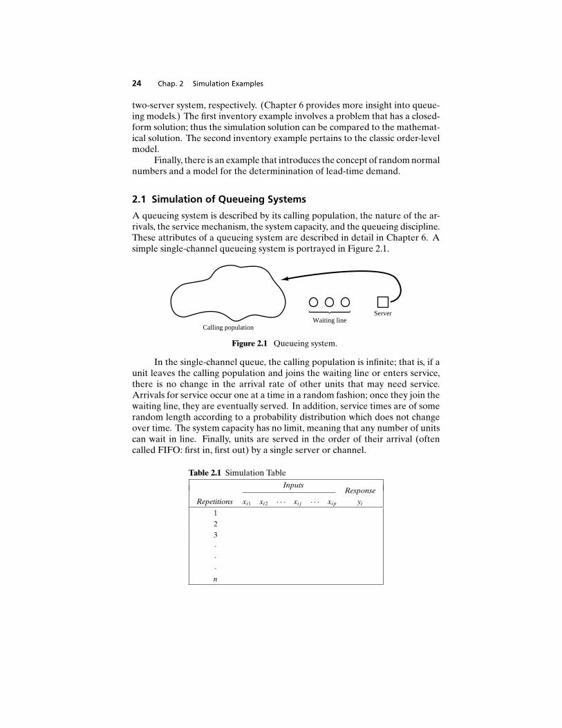
A queueing system is described by its calling population, the nature of the ar-rivals, the service mechanism, the system capacity, and the queueing discipline.These attributes of a queueing system are described in detail in Chapter 6. Asimple single-channel queueing system is portrayed in Figure 2.1.
ServerWaiting line
Calling population
Figure 2.1 Queueing system.
In the single-channel queue, the calling population is infinite; that is, if aunit leaves the calling population and joins the waiting line or enters service,there is no change in the arrival rate of other units that may need service.Arrivals for service occur one at a time in a random fashion; once they join thewaiting line, they are eventually served. In addition, service times are of somerandom length according to a probability distribution which does not changeover time. The system capacity has no limit, meaning that any number of unitscan wait in line. Finally, units are served in the order of their arrival (oftencalled FIFO: first in, first out) by a single server or channel.
Table 2.1 Simulation Table
InputsResponse
Repetitions xi1 xi2 · · · xij · · · xip yi
1
2
3
···n
Sec. 2.1 Simulation of Queueing Systems 25
Arrivals and services are defined by the distribution of the time betweenarrivals and the distribution of service times, respectively. For any simple single-or multi-channel queue, the overall effective arrival rate must be less than thetotal service rate, or the waiting line will grow without bound. When queuesgrow without bound, they are termed “explosive” or unstable. (In some reen-trant queueing networks in which units return a number of times to the sameserver before finally exiting the system, the condition about arrival rate beingless than service rate may not guarantee stability. See Harrison and Nguyen[1995] for more explanation. Interestingly, this type of instability was noticedfirst, not in theory, but in actual manufacturing in semiconductor plants.) Morecomplex situations may occur—for example, arrival rates that are greater thanservice rates for short periods of time, or networks of queues with routing.However, this chapter sticks to the simplest, more basic queues.
Prior to introducing several simulations of queueing systems, it is neces-sary to understand the concepts of system state, events, and simulation clock.(These concepts are studied systematically in Chapter 3.) The state of the sys-tem is the number of units in the system and the status of the server, busy oridle. An event is a set of circumstances that cause an instantaneous change inthe state of the system. In a single-channel queueing system there are only twopossible events that can affect the state of the system. They are the entry of aunit into the system (the arrival event) or the completion of service on a unit(the departure event). The queueing system includes the server, the unit beingserviced (if one is being serviced), and units in the queue (if any are waiting).The simulation clock is used to track simulated time.
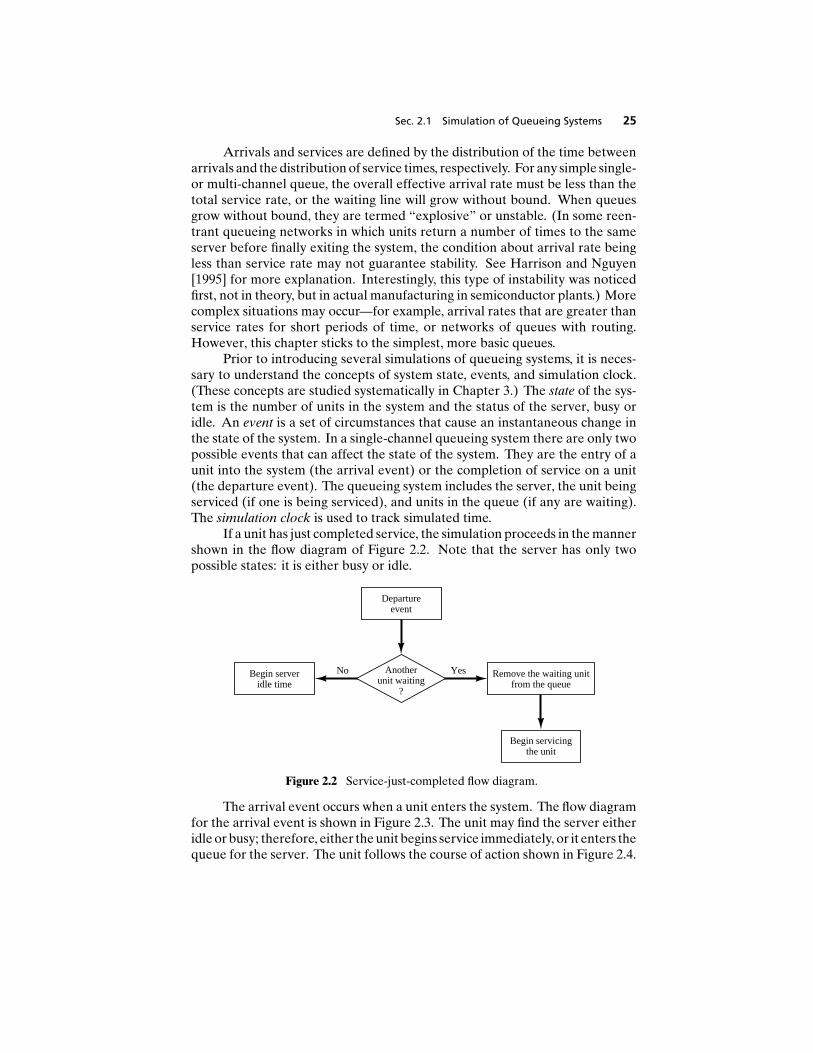
If a unit has just completed service, the simulation proceeds in the mannershown in the flow diagram of Figure 2.2. Note that the server has only twopossible states: it is either busy or idle.
Departureevent
No Yes Remove the waiting unitfrom the queue
Begin servicingthe unit
Begin serveridle time
Anotherunit waiting
?
Figure 2.2 Service-just-completed flow diagram.
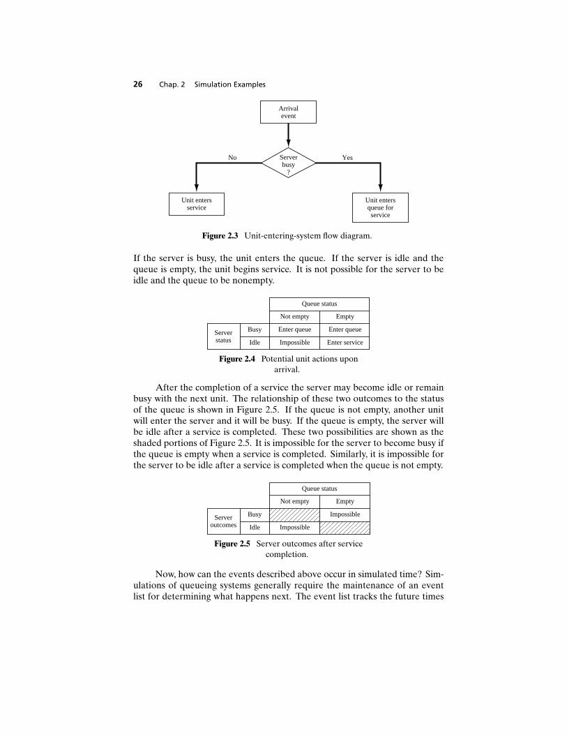
The arrival event occurs when a unit enters the system. The flow diagramfor the arrival event is shown in Figure 2.3. The unit may find the server eitheridle or busy; therefore, either the unit begins service immediately, or it enters thequeue for the server. The unit follows the course of action shown in Figure 2.4.
26 Chap. 2 Simulation Examples
Arrivalevent
Unit entersservice
Unit entersqueue forservice
No YesServerbusy
?
Figure 2.3 Unit-entering-system flow diagram.
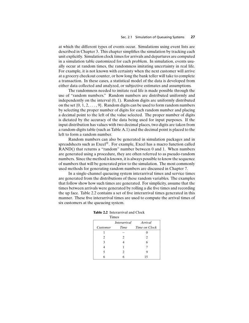
If the server is busy, the unit enters the queue. If the server is idle and thequeue is empty, the unit begins service. It is not possible for the server to beidle and the queue to be nonempty.
Not empty
Enter queue
Impossible
Empty
Enter queue
Enter service
Busy
Idle
Serverstatus
Queue status
Figure 2.4 Potential unit actions uponarrival.
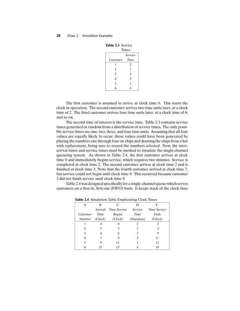
After the completion of a service the server may become idle or remainbusy with the next unit. The relationship of these two outcomes to the statusof the queue is shown in Figure 2.5. If the queue is not empty, another unitwill enter the server and it will be busy. If the queue is empty, the server willbe idle after a service is completed. These two possibilities are shown as theshaded portions of Figure 2.5. It is impossible for the server to become busy ifthe queue is empty when a service is completed. Similarly, it is impossible forthe server to be idle after a service is completed when the queue is not empty.
Not empty
Impossible
Empty
ImpossibleBusy
Idle
Serveroutcomes
Queue status
Figure 2.5 Server outcomes after servicecompletion.
Now, how can the events described above occur in simulated time? Sim-ulations of queueing systems generally require the maintenance of an eventlist for determining what happens next. The event list tracks the future times
Sec. 2.1 Simulation of Queueing Systems 27
at which the different types of events occur. Simulations using event lists aredescribed in Chapter 3. This chapter simplifies the simulation by tracking eachunit explicitly. Simulation clock times for arrivals and departures are computedin a simulation table customized for each problem. In simulation, events usu-ally occur at random times, the randomness imitating uncertainty in real life.For example, it is not known with certainty when the next customer will arriveat a grocery checkout counter, or how long the bank teller will take to completea transaction. In these cases, a statistical model of the data is developed fromeither data collected and analyzed, or subjective estimates and assumptions.
The randomness needed to imitate real life is made possible through theuse of “random numbers.” Random numbers are distributed uniformly andindependently on the interval (0, 1). Random digits are uniformly distributedon the set {0, 1, 2, . . . , 9}. Random digits can be used to form random numbersby selecting the proper number of digits for each random number and placinga decimal point to the left of the value selected. The proper number of digitsis dictated by the accuracy of the data being used for input purposes. If theinput distribution has values with two decimal places, two digits are taken froma random-digits table (such as Table A.1) and the decimal point is placed to theleft to form a random number.
Random numbers can also be generated in simulation packages and inspreadsheets such as Excel®. For example, Excel has a macro function calledRAND() that returns a “random” number between 0 and 1. When numbersare generated using a procedure, they are often referred to as pseudo-randomnumbers. Since the method is known, it is always possible to know the sequenceof numbers that will be generated prior to the simulation. The most commonlyused methods for generating random numbers are discussed in Chapter 7.
In a single-channel queueing system interarrival times and service timesare generated from the distributions of these random variables. The examplesthat follow show how such times are generated. For simplicity, assume that thetimes between arrivals were generated by rolling a die five times and recordingthe up face. Table 2.2 contains a set of five interarrival times generated in thismanner. These five interarrival times are used to compute the arrival times ofsix customers at the queueing system.
Table 2.2 Interarrival and ClockTimes
Interarrival Arrival
Customer Time Time on Clock
1 − 0
2 2 2
3 4 6
4 1 7
5 2 9
6 6 15
28 Chap. 2 Simulation Examples
Table 2.3 ServiceTimes
Service
Customer Time
1 2
2 1
3 3
4 2
5 1
6 4
The first customer is assumed to arrive at clock time 0. This starts theclock in operation. The second customer arrives two time units later, at a clocktime of 2. The third customer arrives four time units later, at a clock time of 6;and so on.
The second time of interest is the service time. Table 2.3 contains servicetimes generated at random from a distribution of service times. The only possi-ble service times are one, two, three, and four time units. Assuming that all fourvalues are equally likely to occur, these values could have been generated byplacing the numbers one through four on chips and drawing the chips from a hatwith replacement, being sure to record the numbers selected. Now, the inter-arrival times and service times must be meshed to simulate the single-channelqueueing system. As shown in Table 2.4, the first customer arrives at clocktime 0 and immediately begins service, which requires two minutes. Service iscompleted at clock time 2. The second customer arrives at clock time 2 and isfinished at clock time 3. Note that the fourth customer arrived at clock time 7,but service could not begin until clock time 9. This occurred because customer3 did not finish service until clock time 9.
Table 2.4 was designed specifically for a single-channel queue which servescustomers on a first-in, first-out (FIFO) basis. It keeps track of the clock time
Table 2.4 Simulation Table Emphasizing Clock Times
A B C D E
Arrival Time Service Service Time Service
Customer Time Begins Time Ends
Number (Clock) (Clock) (Duration) (Clock)
1 0 0 2 2
2 2 2 1 3
3 6 6 3 9
4 7 9 2 11
5 9 11 1 12
6 15 15 4 19

Sec. 2.1 Simulation of Queueing Systems 29
Table 2.5 ChronologicalOrdering ofEvents
Customer Clock
Event Type Number Time
Arrival 1 0
Departure 1 2
Arrival 2 2
Departure 2 3
Arrival 3 6
Arrival 4 7
Departure 3 9
Arrival 5 9
Departure 4 11
Departure 5 12
Arrival 6 15
Departure 6 19
at which each event occurs. The second column of Table 2.4 records the clocktime of each arrival event, while the last column records the clock time of eachdeparture event. The occurrence of the two types of events in chronologicalorder is shown in Table 2.5 and Figure 2.6.
40
1
2
Num
ber
of c
usto
mer
s in
the
syst
tem
8 12 16 20
Clock time
1 2 3 4 5
4 5
6
Figure 2.6 Number of customers in the system.
It should be noted that Table 2.5 is ordered by clock time, in which casethe events may or may not be ordered by customer number. The chronologicalordering of events is the basis of the approach to discrete-event simulationdescribed in Chapter 3.
Figure 2.6 depicts the number of customers in the system at the variousclock times. It is a visual image of the event listing of Table 2.5. Customer 1
30 Chap. 2 Simulation Examples
Table 2.6 Distribution of Time Between Arrivals
Time between
Arrivals Cumulative Random-Digit
(Minutes) Probability Probability Assignment
1 0.125 0.125 001−125
2 0.125 0.250 126−250
3 0.125 0.375 251−375
4 0.125 0.500 376−500
5 0.125 0.625 501−625
6 0.125 0.750 626−750
7 0.125 0.875 751−875
8 0.125 1.000 876−000
is in the system from clock time 0 to clock time 2. Customer 2 arrives at clocktime 2 and departs at clock time 3. No customers are in the system from clocktime 3 to clock time 6. During some time periods two customers are in thesystem, such as at clock time 8, when both customers 3 and 4 are in the system.Also, there are times when events occur simultaneously, such as at clock time9, when customer 5 arrives and customer 3 departs.
Example 2.1 follows the logic described above while keeping track ofa number of attributes of the system. Example 2.2 is concerned with a two-channel queueing system. The flow diagrams for a multichannel queueingsystem are slightly different from those for a single-channel system. The devel-opment and interpretation of these flow diagrams is left as an exercise for thereader.
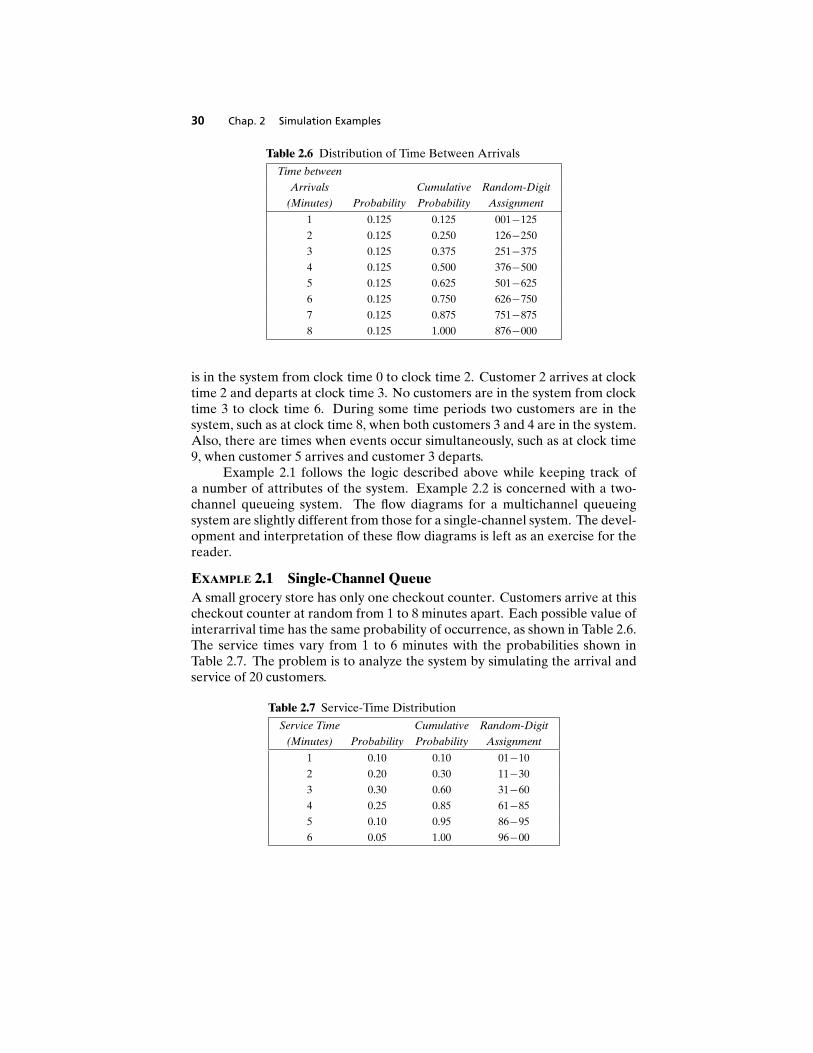
EXAMPLE 2.1 Single-Channel QueueA small grocery store has only one checkout counter. Customers arrive at thischeckout counter at random from 1 to 8 minutes apart. Each possible value ofinterarrival time has the same probability of occurrence, as shown in Table 2.6.The service times vary from 1 to 6 minutes with the probabilities shown inTable 2.7. The problem is to analyze the system by simulating the arrival andservice of 20 customers.
Table 2.7 Service-Time Distribution
Service Time Cumulative Random-Digit
(Minutes) Probability Probability Assignment
1 0.10 0.10 01−10
2 0.20 0.30 11−30
3 0.30 0.60 31−60
4 0.25 0.85 61−85
5 0.10 0.95 86−95
6 0.05 1.00 96−00
Sec. 2.1 Simulation of Queueing Systems 31
In actuality, 20 customers is too small a sample size to allow drawing anyreliable conclusions. The accuracy of the results is enhanced by increasing thesample size, as discussed in Chapter 11. However, the purpose of the exerciseis to demonstrate how simple simulations can be carried out in a table, eithermanually or with a spreadsheet, not to recommend changes in the grocery store.A second issue, discussed thoroughly in Chapter 11, is that of initial conditions.A simulation of a grocery store that starts with an empty system is not realisticunless the intention is to model the system from startup or to model until steady-state operation is reached. Here, to keep things simple, starting conditions andconcerns are overlooked.
A set of uniformly distributed random numbers is needed to generatethe arrivals at the checkout counter. Random numbers have the followingproperties:
1. The set of random numbers is uniformly distributed between 0 and 1.2. Successive random numbers are independent.
With tabular simulations, random digits such as those found in Table A.1 inthe Appendix can be converted to random numbers. If using a spreadsheet,most have a built-in random-number generator such as RAND() in Excel. Theexample in the text uses random digits from Table A.1; in some of the exercisesthe student is asked to use a spreadsheet.
Random digits are converted to random numbers by placing a decimalpoint appropriately. Since the probabilities in Table 2.6 are accurate to 3 signif-icant digits, three-place random numbers will suffice. It is necessary to list only19 random numbers to generate times between arrivals. Why only 19 numbers?The first arrival is assumed to occur at time 0, so only 19 more arrivals need tobe generated to end up with 20 customers. Similarly, for Table 2.7, two-placerandom numbers will suffice.
The rightmost two columns of Tables 2.6 and 2.7 are used to generate ran-dom arrivals and random service times. The third column in each table containsthe cumulative probability for the distribution. The rightmost column containsthe random digit-assignment. In Table 2.6, the first random-digit assignmentis 001–125. There are 1000 three-digit values possible (001 through 000). Theprobability of a time-between-arrivals of 1 minute is 0.125, and 125 of the 1000random-digit values are assigned to such an occurrence. Times between ar-rivals for 19 customers are generated by listing 19 three-digit values from TableA.1 and comparing them to the random-digit assignment of Table 2.6.
For manual simulations, it is good practice to start at a random position inthe random-digit table and proceed in a systematic direction, never re-using thesame stream of digits in a given problem. If the same pattern is used repeatedly,bias could result, because the same event pattern would be generated. In Excel,each time the random function RAND() is evaluated, it returns a new randomvalue.
The time-between-arrival determination is shown in Table 2.8. Note thatthe first random digits are 913. To obtain the corresponding time between

32 Chap. 2 Simulation Examples
Table 2.8 Time-Between-Arrivals Determination
Time between Time between
Random Arrivals Random Arrivals
Customer Digits (Minutes) Customer Digits (Minutes)
1 − − 11 109 1
2 913 8 12 093 1
3 727 6 13 607 5
4 015 1 14 738 6
5 948 8 15 359 3
6 309 3 16 888 8
7 922 8 17 106 1
8 753 7 18 212 2
9 235 2 19 493 4
10 302 3 20 535 5
arrivals, enter the fourth column of Table 2.6 and read 8 minutes from the firstcolumn of the table. Alternatively, we see that 0.913 is between the cumulativeprobabilities 0.876 and 1.000, again resulting in 8 minutes as the generated time.
Service times for all 20 customers are shown in Table 2.9. These servicetimes were generated based on the methodology described above, together withthe aid of Table 2.7. The first customer’s service time is 4 minutes because therandom digits 84 fall in the bracket 61–85, or alternatively because the derivedrandom number 0.84 falls between the cumulative probabilities 0.61 and 0.85.
Table 2.9 Service Times Generated
Service Service
Random Time Random Time
Customer Digits (Minutes) Customer Digits (Minutes)
1 84 4 11 32 3
2 10 1 12 94 5
3 74 4 13 79 4
4 53 3 14 05 1
5 17 2 15 79 5
6 79 4 16 84 4
7 91 5 17 52 3
8 67 4 18 55 3
9 89 5 19 30 2
10 38 3 20 50 3
Sec. 2.1 Simulation of Queueing Systems 33
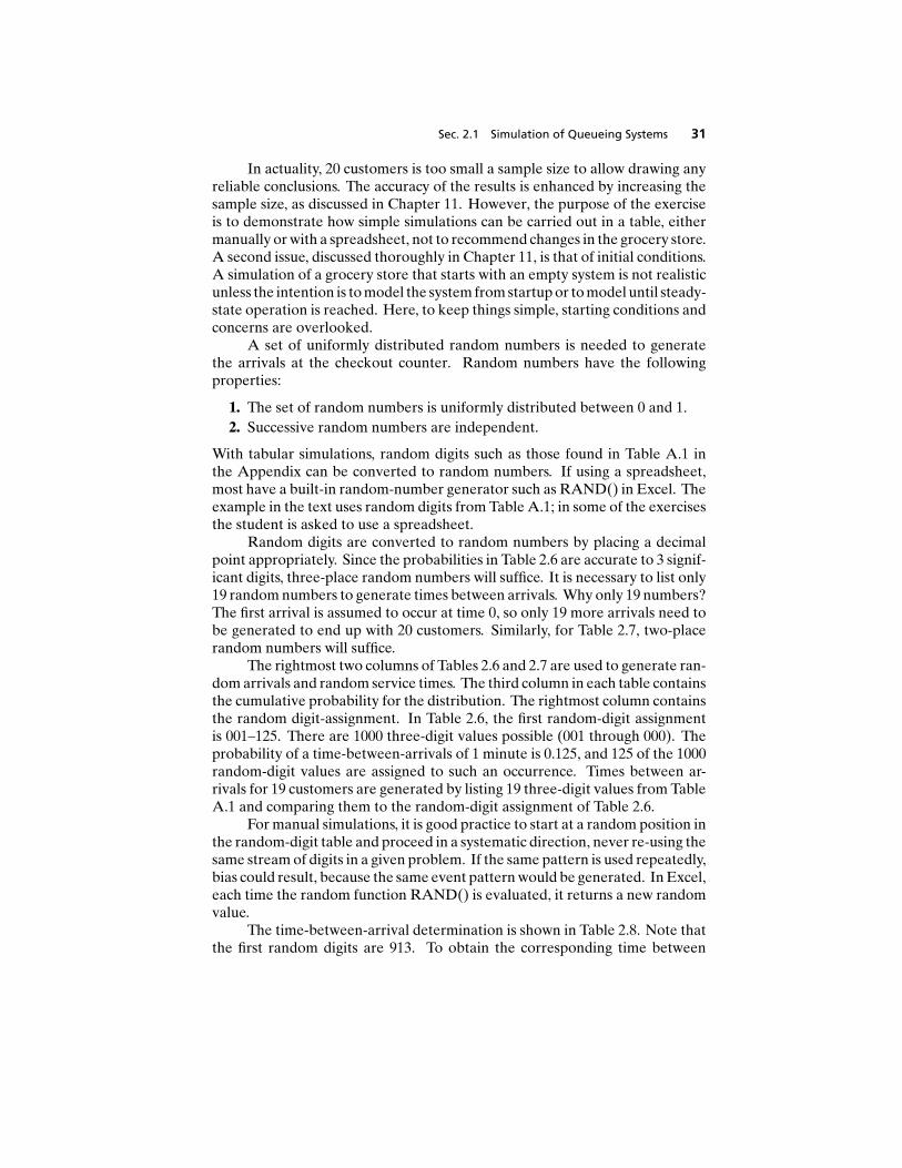
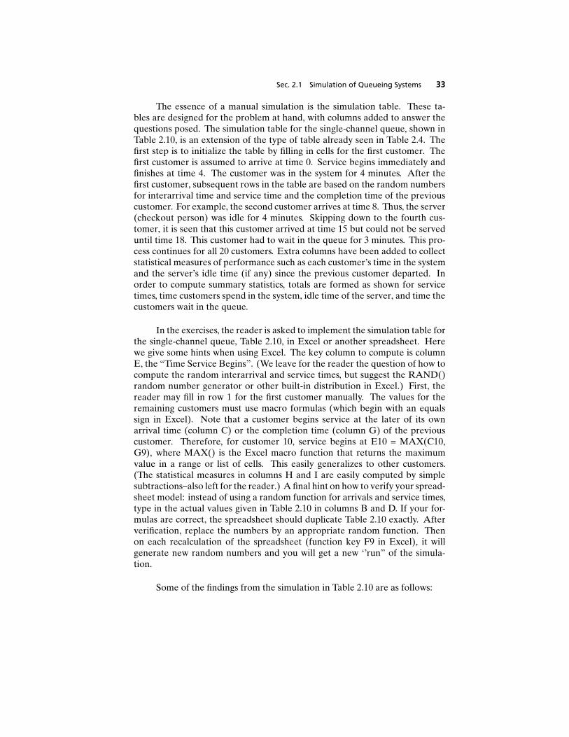
The essence of a manual simulation is the simulation table. These ta-bles are designed for the problem at hand, with columns added to answer thequestions posed. The simulation table for the single-channel queue, shown inTable 2.10, is an extension of the type of table already seen in Table 2.4. Thefirst step is to initialize the table by filling in cells for the first customer. Thefirst customer is assumed to arrive at time 0. Service begins immediately andfinishes at time 4. The customer was in the system for 4 minutes. After thefirst customer, subsequent rows in the table are based on the random numbersfor interarrival time and service time and the completion time of the previouscustomer. For example, the second customer arrives at time 8. Thus, the server(checkout person) was idle for 4 minutes. Skipping down to the fourth cus-tomer, it is seen that this customer arrived at time 15 but could not be serveduntil time 18. This customer had to wait in the queue for 3 minutes. This pro-cess continues for all 20 customers. Extra columns have been added to collectstatistical measures of performance such as each customer’s time in the systemand the server’s idle time (if any) since the previous customer departed. Inorder to compute summary statistics, totals are formed as shown for servicetimes, time customers spend in the system, idle time of the server, and time thecustomers wait in the queue.
In the exercises, the reader is asked to implement the simulation table forthe single-channel queue, Table 2.10, in Excel or another spreadsheet. Herewe give some hints when using Excel. The key column to compute is columnE, the “Time Service Begins”. (We leave for the reader the question of how tocompute the random interarrival and service times, but suggest the RAND()random number generator or other built-in distribution in Excel.) First, thereader may fill in row 1 for the first customer manually. The values for theremaining customers must use macro formulas (which begin with an equalssign in Excel). Note that a customer begins service at the later of its ownarrival time (column C) or the completion time (column G) of the previouscustomer. Therefore, for customer 10, service begins at E10 = MAX(C10,G9), where MAX() is the Excel macro function that returns the maximumvalue in a range or list of cells. This easily generalizes to other customers.(The statistical measures in columns H and I are easily computed by simplesubtractions–also left for the reader.) A final hint on how to verify your spread-sheet model: instead of using a random function for arrivals and service times,type in the actual values given in Table 2.10 in columns B and D. If your for-mulas are correct, the spreadsheet should duplicate Table 2.10 exactly. Afterverification, replace the numbers by an appropriate random function. Thenon each recalculation of the spreadsheet (function key F9 in Excel), it willgenerate new random numbers and you will get a new ‘’run” of the simula-tion.
Some of the findings from the simulation in Table 2.10 are as follows:

34 Chap. 2 Simulation Examples
1. The average waiting time for a customer is 2.8 minutes. This is determinedin the following manner:
average waiting time(minutes)
= total time customers wait in queue (minutes)total numbers of customers
= 5620
= 2.8 minutes
2. The probability that a customer has to wait in the queue is 0.65. This isdetermined in the following manner:
probability (wait) = number of customers who waittotal number of customers
= 1320
= 0.65
3. The fraction of idle time of the server is 0.21. This is determined in thefollowing manner:
probability of idleserver
= total idle time of server (minutes)total run time of simulation (minutes)
= 1886
= 0.21
The probability of the server being busy is the complement of 0.21, or0.79.
4. The average service time is 3.4 minutes, determined as follows:
average service time(minutes)
= total service time (minutes)total number of customers
= 6820
= 3.4 minutes
This result can be compared with the expected service time by finding themean of the service-time distribution using the equation
E(S) =∞∑
s=0
sp(s)
Applying the expected-value equation to the distribution in Table 2.7gives an expected service time of:
= 1(0.10) + 2(0.20) + 3(0.30) + 4(0.25) + 5(0.10) + 6(0.05)
= 3.2 minutes
The expected service time is slightly lower than the average service timein the simulation. The longer the simulation, the closer the average willbe to E(S).
Sec.2.1Sim
ulatio
no
fQ
ueu
eing
Systems
35
Table 2.10 Simulation Table for Queueing Problem
A B C D E F G H ITime Since Service Time Time Customer Time Time Customer Idle TimeLast Arrival Arrival Time Service Waits in Queue Service Spends in System of Server
Customer (Minutes) Time (Minutes) Begins (Minutes) Ends (Minutes) (Minutes)1 − 0 4 0 0 4 4 02 8 8 1 8 0 9 1 43 6 14 4 14 0 18 4 54 1 15 3 18 3 21 6 05 8 23 2 23 0 25 2 26 3 26 4 26 0 30 4 17 8 34 5 34 0 39 5 48 7 41 4 41 0 45 4 29 2 43 5 45 2 50 7 0
10 3 46 3 50 4 53 7 011 1 47 3 53 6 56 9 012 1 48 5 56 8 61 13 013 5 53 4 61 8 65 12 014 6 59 1 65 6 66 7 015 3 62 5 66 4 71 9 016 8 70 4 71 1 75 5 017 1 71 3 75 4 78 7 018 2 73 3 78 5 81 8 019 4 77 2 81 4 83 6 020 5 82 3 83 1 86 4 0
68 56 124 18
36 Chap. 2 Simulation Examples
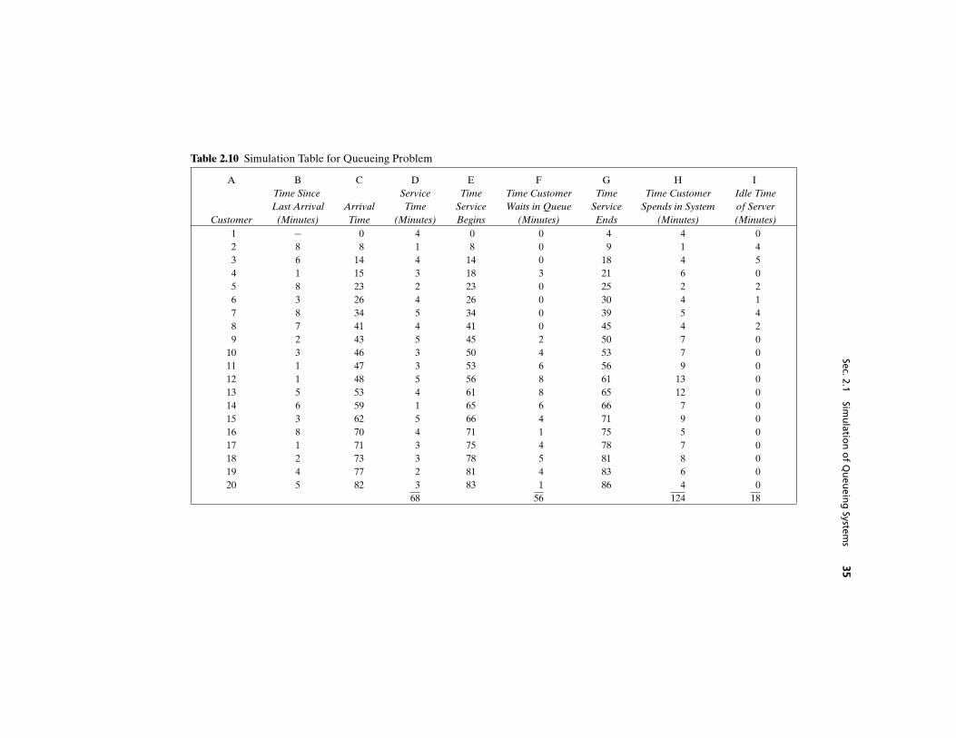
5. The average time between arrivals is 4.3 minutes. This is determined inthe following manner:
average time betweenarrivals (minutes)
=sum of all times
between arrivals (minutes)number of arrivals −1
= 8219
= 4.3 minutes
One is subtracted from the denominator because the first arrival is as-sumed to occur at time 0. This result can be compared to the expectedtime between arrivals by finding the mean of the discrete uniform dis-tribution whose endpoints are a = 1 and b = 8. The mean is givenby
E(A) = a + b
2= 1 + 8
2= 4.5 minutes
The expected time between arrivals is slightly higher than the average.However, as the simulation becomes longer, the average value of the timebetween arrivals will approach the theoretical mean, E(A).
6. The average waiting time of those who wait is 4.3 minutes. This is deter-mined in the following manner:
Average waiting time ofthose who wait (minutes)
= total time customers wait in queue (minutes)total number of customers who wait
= 5613
= 4.3 minutes
7. The average time a customer spends in the system is 6.2 minutes. Thiscan be determined in two ways. First, the computation can be achievedby the following relationship:
average time customer
spends in the system
(minutes)
=total time customers spend in the
system (minutes)total number of customers
= 12420
= 6.2 minutes
The second way of computing this same result is to realize that the fol-lowing relationship must hold:
average time average time average timecustomer spends customer spends customer spends
in the system = waiting in the + in service(minutes) queue (minutes) (minutes)
Sec. 2.1 Simulation of Queueing Systems 37
From findings 1 and 4 this results in:
Average time customer spends in the system (minutes)
= 2.8 + 3.4 = 6.2 minutes
A decision maker would be interested in results of this type, but a longersimulation would increase the accuracy of the findings. However, some sub-jective inferences can be drawn at this point. Most customers have to wait;however, the average waiting time is not excessive. The server does not havean undue amount of idle time. Objective statements about the results woulddepend on balancing the cost of waiting with the cost of additional servers.(Simulations requiring variations of the arrival and service distributions, aswell as implementation in a spreadsheet, are presented as exercises for thereader.) m
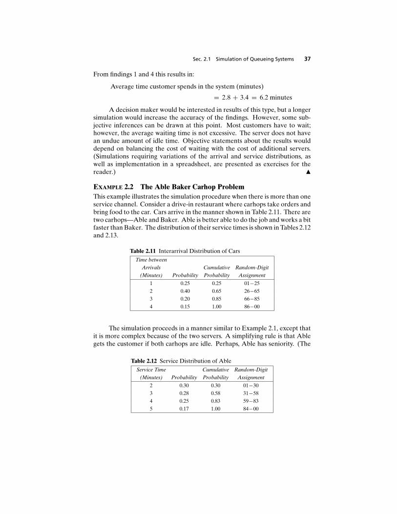
EXAMPLE 2.2 The Able Baker Carhop ProblemThis example illustrates the simulation procedure when there is more than oneservice channel. Consider a drive-in restaurant where carhops take orders andbring food to the car. Cars arrive in the manner shown in Table 2.11. There aretwo carhops—Able and Baker. Able is better able to do the job and works a bitfaster than Baker. The distribution of their service times is shown in Tables 2.12and 2.13.
Table 2.11 Interarrival Distribution of Cars
Time between
Arrivals Cumulative Random-Digit
(Minutes) Probability Probability Assignment
1 0.25 0.25 01−25
2 0.40 0.65 26−65
3 0.20 0.85 66−85
4 0.15 1.00 86−00
The simulation proceeds in a manner similar to Example 2.1, except thatit is more complex because of the two servers. A simplifying rule is that Ablegets the customer if both carhops are idle. Perhaps, Able has seniority. (The
Table 2.12 Service Distribution of Able
Service Time Cumulative Random-Digit
(Minutes) Probability Probability Assignment
2 0.30 0.30 01−30
3 0.28 0.58 31−58
4 0.25 0.83 59−83
5 0.17 1.00 84−00
38 Chap. 2 Simulation Examples
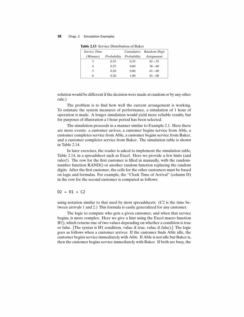
Table 2.13 Service Distribution of Baker
Service Time Cumulative Random-Digit
(Minutes) Probability Probability Assignment
3 0.35 0.35 01−35
4 0.25 0.60 36−60
5 0.20 0.80 61−80
6 0.20 1.00 81−00
solution would be different if the decision were made at random or by any otherrule.)
The problem is to find how well the current arrangement is working.To estimate the system measures of performance, a simulation of 1 hour ofoperation is made. A longer simulation would yield more reliable results, butfor purposes of illustration a l-hour period has been selected.
The simulation proceeds in a manner similar to Example 2.1. Here thereare more events: a customer arrives, a customer begins service from Able, acustomer completes service from Able, a customer begins service from Baker,and a customer completes service from Baker. The simulation table is shownin Table 2.14.
In later exercises, the reader is asked to implement the simulation table,Table 2.14, in a spreadsheet such as Excel. Here we provide a few hints (andrules!). The row for the first customer is filled in manually, with the random-number function RAND() or another random function replacing the randomdigits. After the first customer, the cells for the other customers must be basedon logic and formulas. For example, the “Clock Time of Arrival” (column D)in the row for the second customer is computed as follows:
D2 = D1 + C2
using notation similar to that used by most spreadsheets. (C2 is the time be-tween arrivals 1 and 2.) This formula is easily generalized for any customer.
The logic to compute who gets a given customer, and when that servicebegins, is more complex. Here we give a hint using the Excel macro functionIF(), which returns one of two values depending on whether a condition is trueor false. [The syntax is IF( condition, value if true, value if false).] The logicgoes as follows when a customer arrives: If the customer finds Able idle, thecustomer begins service immediately with Able. If Able is not idle but Baker is,then the customer begins service immediately with Baker. If both are busy, the
Sec. 2.1 Simulation of Queueing Systems 39
customer begins service with the first server to become free. The logic requiresthat we compute when Able and Baker will become free, for which we use thebuilt-in Excel function for maximum over a range, MAX(). For example, forcustomer 10, Able will become free at MAX(H$1:H9), since service comple-tion time is in column H and we need to look at customers 1–9. (Using H$1instead of H1 works better with Excel when formulas are copied. The dollarsign indicates an absolute reference versus a relative reference to a cell.) Theresulting formula to compute whether and when Able serves customer 10 is asfollows:
F10 = IF(D10>MAX(H$1:H9),D10, IF(D10>MAX(K$1:K9),’’’’,MIN(MAX(H$1:H9),MAX(K$1:K9))))
In this formula, note that if the first condition (Able idle when customer 10arrives) is true, then the customer begins immediately at the arrival time inD10. Otherwise, a second IF() function is evaluated, which says if Baker isidle, put nothing (“”) in the cell. Otherwise, the function returns the time thatAble or Baker becomes idle, whichever is first [the minimum or MIN() of theirrespective completion times]. A similar formula applies to cell I10 for “TimeService Begins” for Baker. For service times for Able, you could use anotherIF() function to make the cell blank or have a value:
G10 = IF(F10 > 0,new service time, "")H10 = IF(F10 > 0, F10+G10, "")
and similarly for Baker. With these hints, we leave the formula fornew service time as well as the remainder of the solution to the reader.
The analysis of Table 2.14 results in the following:
1. Over the 62-minute period Able was busy 90% of the time.
2. Baker was busy only 69% of the time. The seniority rule keeps Baker lessbusy (and gives Able more tips).
3. Nine of the 26 arrivals (about 35%) had to wait. The average waiting timefor all customers was only about 0.42 minute (25 seconds), which is verysmall.
4. Those nine who did have to wait only waited an average of 1.22 minutes,which is quite low.
5. In summary, this system seems well balanced. One server cannot handleall the diners, and three servers would probably be too many. Addingan additional server would surely reduce the waiting time to nearly zero.However, the cost of waiting would have to be quite high to justify anadditional server. m
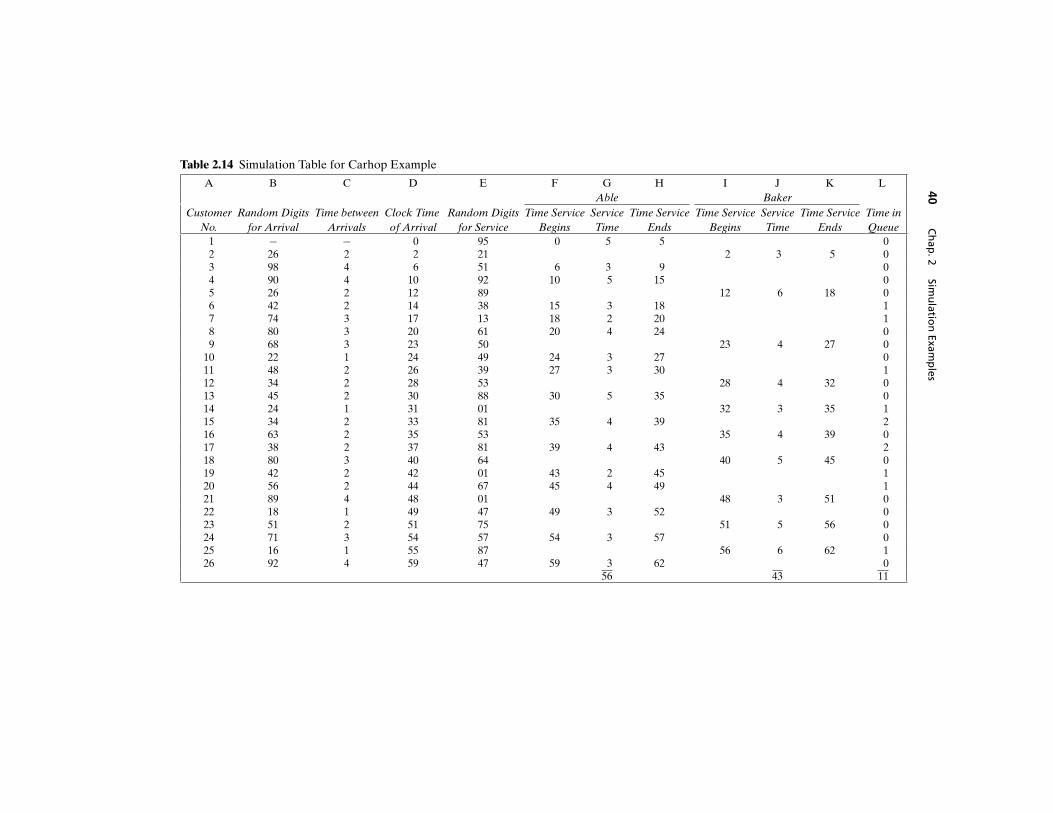
40C
hap
.2Sim
ulatio
nExam
ples
Table 2.14 Simulation Table for Carhop Example
A B C D E F G H I J K LAble Baker
Customer Random Digits Time between Clock Time Random Digits Time Service Service Time Service Time Service Service Time Service Time inNo. for Arrival Arrivals of Arrival for Service Begins Time Ends Begins Time Ends Queue
1 − − 0 95 0 5 5 02 26 2 2 21 2 3 5 03 98 4 6 51 6 3 9 04 90 4 10 92 10 5 15 05 26 2 12 89 12 6 18 06 42 2 14 38 15 3 18 17 74 3 17 13 18 2 20 18 80 3 20 61 20 4 24 09 68 3 23 50 23 4 27 0
10 22 1 24 49 24 3 27 011 48 2 26 39 27 3 30 112 34 2 28 53 28 4 32 013 45 2 30 88 30 5 35 014 24 1 31 01 32 3 35 115 34 2 33 81 35 4 39 216 63 2 35 53 35 4 39 017 38 2 37 81 39 4 43 218 80 3 40 64 40 5 45 019 42 2 42 01 43 2 45 120 56 2 44 67 45 4 49 121 89 4 48 01 48 3 51 022 18 1 49 47 49 3 52 023 51 2 51 75 51 5 56 024 71 3 54 57 54 3 57 025 16 1 55 87 56 6 62 126 92 4 59 47 59 3 62 0
56 43 11
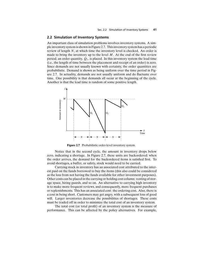
Sec. 2.2 Simulation of Inventory Systems 41
2.2 Simulation of Inventory Systems
An important class of simulation problems involves inventory systems. A sim-ple inventory system is shown in Figure 2.7. This inventory system has a periodicreview of length N , at which time the inventory level is checked. An order ismade to bring the inventory up to the level M . At the end of the first reviewperiod, an order quantity, Q1, is placed. In this inventory system the lead time(i.e., the length of time between the placement and receipt of an order) is zero.Since demands are not usually known with certainty, the order quantities areprobabilistic. Demand is shown as being uniform over the time period in Fig-ure 2.7. In actuality, demands are not usually uniform and do fluctuate overtime. One possibility is that demands all occur at the beginning of the cycle.Another is that the lead time is random of some positive length.
M
Am
ount
in in
vent
ory
TTime
I
N N N
Q1 Q2
Q3
Figure 2.7 Probabilistic order-level inventory system.
Notice that in the second cycle, the amount in inventory drops belowzero, indicating a shortage. In Figure 2.7, these units are backordered; whenthe order arrives, the demand for the backordered items is satisfied first. Toavoid shortages, a buffer, or safety, stock would need to be carried.
Carrying stock in inventory has an associated cost attributed to the inter-est paid on the funds borrowed to buy the items (this also could be consideredas the loss from not having the funds available for other investment purposes).Other costs can be placed in the carrying or holding cost column: renting of stor-age space, hiring guards, and so on. An alternative to carrying high inventoryis to make more frequent reviews, and consequently, more frequent purchasesor replenishments. This has an associated cost: the ordering cost. Also, there isa cost in being short. Customers may get angry, with a subsequent loss of goodwill. Larger inventories decrease the possibilities of shortages. These costsmust be traded off in order to minimize the total cost of an inventory system.
The total cost (or total profit) of an inventory system is the measure ofperformance. This can be affected by the policy alternatives. For example,
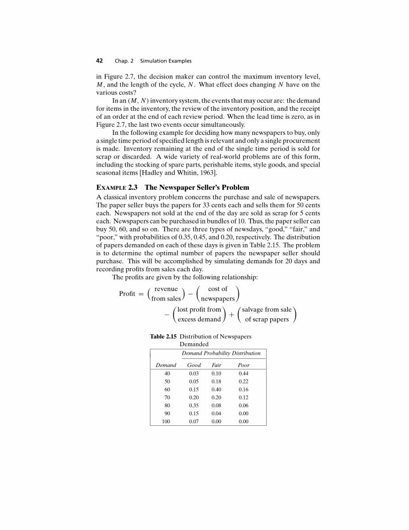
42 Chap. 2 Simulation Examples
in Figure 2.7, the decision maker can control the maximum inventory level,M , and the length of the cycle, N . What effect does changing N have on thevarious costs?
In an (M, N) inventory system, the events that may occur are: the demandfor items in the inventory, the review of the inventory position, and the receiptof an order at the end of each review period. When the lead time is zero, as inFigure 2.7, the last two events occur simultaneously.
In the following example for deciding how many newspapers to buy, onlya single time period of specified length is relevant and only a single procurementis made. Inventory remaining at the end of the single time period is sold forscrap or discarded. A wide variety of real-world problems are of this form,including the stocking of spare parts, perishable items, style goods, and specialseasonal items [Hadley and Whitin, 1963].
EXAMPLE 2.3 The Newspaper Seller’s ProblemA classical inventory problem concerns the purchase and sale of newspapers.The paper seller buys the papers for 33 cents each and sells them for 50 centseach. Newspapers not sold at the end of the day are sold as scrap for 5 centseach. Newspapers can be purchased in bundles of 10. Thus, the paper seller canbuy 50, 60, and so on. There are three types of newsdays, “good,” “fair,” and“poor,” with probabilities of 0.35, 0.45, and 0.20, respectively. The distributionof papers demanded on each of these days is given in Table 2.15. The problemis to determine the optimal number of papers the newspaper seller shouldpurchase. This will be accomplished by simulating demands for 20 days andrecording profits from sales each day.
The profits are given by the following relationship:
Profit =( revenue
from sales
)−
(cost of
newspapers
)
−(
lost profit fromexcess demand
)+
(salvage from saleof scrap papers
)
Table 2.15 Distribution of NewspapersDemanded
Demand Probability Distribution
Demand Good Fair Poor
40 0.03 0.10 0.44
50 0.05 0.18 0.22
60 0.15 0.40 0.16
70 0.20 0.20 0.12
80 0.35 0.08 0.06
90 0.15 0.04 0.00
100 0.07 0.00 0.00
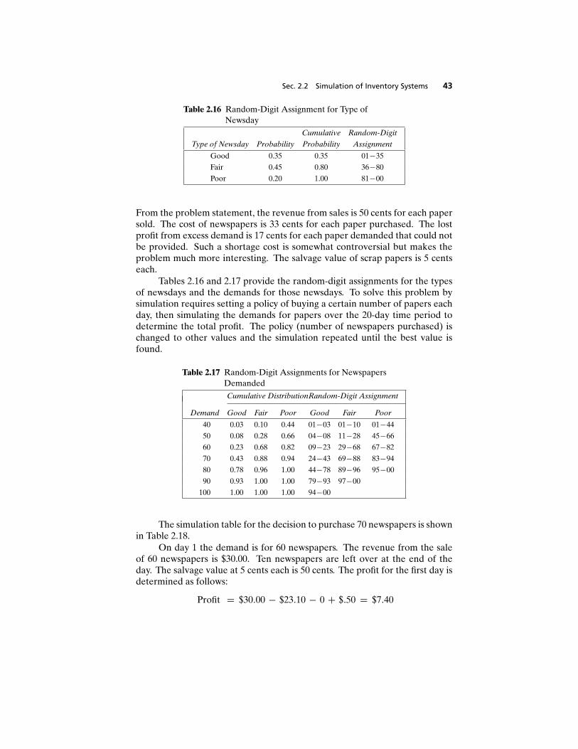
Sec. 2.2 Simulation of Inventory Systems 43
Table 2.16 Random-Digit Assignment for Type ofNewsday
Cumulative Random-Digit
Type of Newsday Probability Probability Assignment
Good 0.35 0.35 01−35
Fair 0.45 0.80 36−80
Poor 0.20 1.00 81−00
From the problem statement, the revenue from sales is 50 cents for each papersold. The cost of newspapers is 33 cents for each paper purchased. The lostprofit from excess demand is 17 cents for each paper demanded that could notbe provided. Such a shortage cost is somewhat controversial but makes theproblem much more interesting. The salvage value of scrap papers is 5 centseach.
Tables 2.16 and 2.17 provide the random-digit assignments for the typesof newsdays and the demands for those newsdays. To solve this problem bysimulation requires setting a policy of buying a certain number of papers eachday, then simulating the demands for papers over the 20-day time period todetermine the total profit. The policy (number of newspapers purchased) ischanged to other values and the simulation repeated until the best value isfound.
Table 2.17 Random-Digit Assignments for NewspapersDemanded
Cumulative DistributionRandom-Digit Assignment
Demand Good Fair Poor Good Fair Poor
40 0.03 0.10 0.44 01−03 01−10 01−44
50 0.08 0.28 0.66 04−08 11−28 45−66
60 0.23 0.68 0.82 09−23 29−68 67−82
70 0.43 0.88 0.94 24−43 69−88 83−94
80 0.78 0.96 1.00 44−78 89−96 95−00
90 0.93 1.00 1.00 79−93 97−00
100 1.00 1.00 1.00 94−00
The simulation table for the decision to purchase 70 newspapers is shownin Table 2.18.
On day 1 the demand is for 60 newspapers. The revenue from the saleof 60 newspapers is $30.00. Ten newspapers are left over at the end of theday. The salvage value at 5 cents each is 50 cents. The profit for the first day isdetermined as follows:
Profit = $30.00 − $23.10 − 0 + $.50 = $7.40

44C
hap
.2Sim
ulatio
nExam
ples
Table 2.18 Simulation Table for Purchase of 70 Newspapers
Random
Digits for Random Revenue Lost Profit Salvage
Type of Type of Digits for from from Excess from Sale Daily
Day Newsday Newsday Demand Demand Sales Demand of Scrap Profit
1 94 Poor 80 60 $30.00 − $0.50 $7.40
2 77 Fair 20 50 25.00 − 1.00 2.90
3 49 Fair 15 50 25.00 − 1.00 2.90
4 45 Fair 88 70 35.00 − − 11.90
5 43 Fair 98 90 35.00 $3.40 − 8.50
6 32 Good 65 80 35.00 1.70 − 10.20
7 49 Fair 86 70 35.00 − − 11.90
8 00 Poor 73 60 30.00 − 0.50 7.40
9 16 Good 24 70 35.00 − − 11.90
10 24 Good 60 80 35.00 1.70 − 10.20
11 31 Good 60 80 35.00 1.70 − 10.20
12 14 Good 29 70 35.00 − − 11.90
13 41 Fair 18 50 25.00 − 1.00 2.90
14 61 Fair 90 80 35.00 1.70 − 10.20
15 85 Poor 93 70 35.00 − − 11.90
16 08 Good 73 80 35.00 1.70 − 10.20
17 15 Good 21 60 30.00 − 0.50 7.40
18 97 Poor 45 50 25.00 − 1.00 2.90
19 52 Fair 76 70 35.00 − − 11.90
20 78 Fair 96 80 35.00 1.70 − 10.20
$645.00 $13.60 $5.50 $174.90
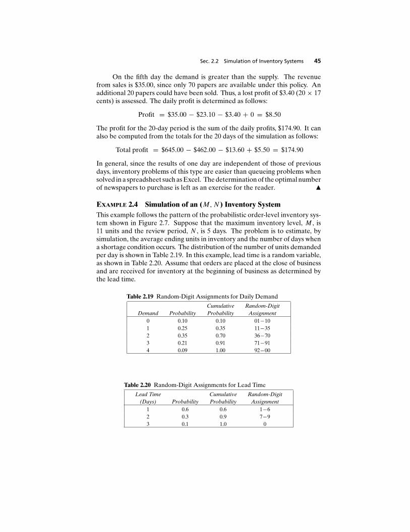
Sec. 2.2 Simulation of Inventory Systems 45
On the fifth day the demand is greater than the supply. The revenuefrom sales is $35.00, since only 70 papers are available under this policy. Anadditional 20 papers could have been sold. Thus, a lost profit of $3.40 (20 × 17cents) is assessed. The daily profit is determined as follows:
Profit = $35.00 − $23.10 − $3.40 + 0 = $8.50
The profit for the 20-day period is the sum of the daily profits, $174.90. It canalso be computed from the totals for the 20 days of the simulation as follows:
Total profit = $645.00 − $462.00 − $13.60 + $5.50 = $174.90
In general, since the results of one day are independent of those of previousdays, inventory problems of this type are easier than queueing problems whensolved in a spreadsheet such as Excel. The determination of the optimal numberof newspapers to purchase is left as an exercise for the reader. m
EXAMPLE 2.4 Simulation of an (M, N ) Inventory SystemThis example follows the pattern of the probabilistic order-level inventory sys-tem shown in Figure 2.7. Suppose that the maximum inventory level, M , is11 units and the review period, N , is 5 days. The problem is to estimate, bysimulation, the average ending units in inventory and the number of days whena shortage condition occurs. The distribution of the number of units demandedper day is shown in Table 2.19. In this example, lead time is a random variable,as shown in Table 2.20. Assume that orders are placed at the close of businessand are received for inventory at the beginning of business as determined bythe lead time.
Table 2.19 Random-Digit Assignments for Daily Demand
Cumulative Random-DigitDemand Probability Probability Assignment
0 0.10 0.10 01−101 0.25 0.35 11−352 0.35 0.70 36−703 0.21 0.91 71−914 0.09 1.00 92−00
Table 2.20 Random-Digit Assignments for Lead Time
Lead Time Cumulative Random-Digit(Days) Probability Probability Assignment
1 0.6 0.6 1−62 0.3 0.9 7−93 0.1 1.0 0
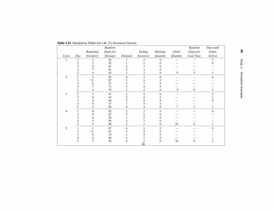
46C
hap
.2Sim
ulatio
nExam
ples
Table 2.21 Simulation Tables for (M, N ) Inventory System
Random Random Days until
Beginning Digits for Ending Shortage Order Digits for Order
Cycle Day Inventory Demand Demand Inventory Quantity Quantity Lead Time Arrives
1 1 3 24 1 2 0 − − 12 2 35 1 1 0 − − 03 9 65 2 7 0 − − −4 7 81 3 4 0 − − −5 4 54 2 2 0 9 5 1
2 1 2 03 0 2 0 − − 02 11 87 3 8 0 − − −3 8 27 1 7 0 − − −4 7 73 3 4 0 − − −5 4 70 2 2 0 9 0 3
3 1 2 47 2 0 0 − − 22 0 45 2 0 2 − − 13 0 48 2 0 4 − − 04 9 17 1 4 0 − − −5 4 09 0 4 0 7 3 1
4 1 4 42 2 2 0 − − 02 9 87 3 6 0 − − −3 6 26 1 5 0 − − −4 5 36 2 3 0 − − −5 3 40 2 1 0 10 4 1
5 1 1 07 0 1 0 − − 02 11 63 2 9 0 − − −3 9 19 1 8 0 − − −4 8 88 3 5 0 − − −5 5 94 4 1 0 10 8 2
88
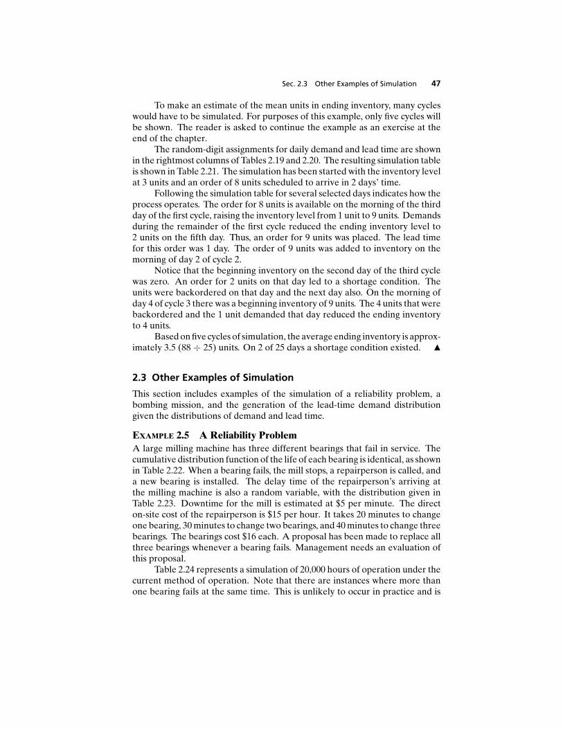
Sec. 2.3 Other Examples of Simulation 47
To make an estimate of the mean units in ending inventory, many cycleswould have to be simulated. For purposes of this example, only five cycles willbe shown. The reader is asked to continue the example as an exercise at theend of the chapter.
The random-digit assignments for daily demand and lead time are shownin the rightmost columns of Tables 2.19 and 2.20. The resulting simulation tableis shown in Table 2.21. The simulation has been started with the inventory levelat 3 units and an order of 8 units scheduled to arrive in 2 days’ time.
Following the simulation table for several selected days indicates how theprocess operates. The order for 8 units is available on the morning of the thirdday of the first cycle, raising the inventory level from 1 unit to 9 units. Demandsduring the remainder of the first cycle reduced the ending inventory level to2 units on the fifth day. Thus, an order for 9 units was placed. The lead timefor this order was 1 day. The order of 9 units was added to inventory on themorning of day 2 of cycle 2.
Notice that the beginning inventory on the second day of the third cyclewas zero. An order for 2 units on that day led to a shortage condition. Theunits were backordered on that day and the next day also. On the morning ofday 4 of cycle 3 there was a beginning inventory of 9 units. The 4 units that werebackordered and the 1 unit demanded that day reduced the ending inventoryto 4 units.
Based on five cycles of simulation, the average ending inventory is approx-imately 3.5 (88 ÷ 25) units. On 2 of 25 days a shortage condition existed. m
2.3 Other Examples of Simulation
This section includes examples of the simulation of a reliability problem, abombing mission, and the generation of the lead-time demand distributiongiven the distributions of demand and lead time.
EXAMPLE 2.5 A Reliability ProblemA large milling machine has three different bearings that fail in service. Thecumulative distribution function of the life of each bearing is identical, as shownin Table 2.22. When a bearing fails, the mill stops, a repairperson is called, anda new bearing is installed. The delay time of the repairperson’s arriving atthe milling machine is also a random variable, with the distribution given inTable 2.23. Downtime for the mill is estimated at $5 per minute. The directon-site cost of the repairperson is $15 per hour. It takes 20 minutes to changeone bearing, 30 minutes to change two bearings, and 40 minutes to change threebearings. The bearings cost $16 each. A proposal has been made to replace allthree bearings whenever a bearing fails. Management needs an evaluation ofthis proposal.
Table 2.24 represents a simulation of 20,000 hours of operation under thecurrent method of operation. Note that there are instances where more thanone bearing fails at the same time. This is unlikely to occur in practice and is

48 Chap. 2 Simulation Examples
Table 2.22 Bearing-Life Distribution
Bearing
Life Cumulative Random-Digit
(Hours) Probability Probability Assignment
1000 0.10 0.10 01−10
1100 0.13 0.23 11−23
1200 0.25 0.48 24−48
1300 0.13 0.61 49−61
1400 0.09 0.70 62−70
1500 0.12 0.82 71−82
1600 0.02 0.84 83−84
1700 0.06 0.90 85−90
1800 0.05 0.95 91−95
1900 0.05 1.00 96−00
due to using a rather coarse grid of 100 hours. It will be assumed in this examplethat the times are never exactly the same, and thus no more than one bearing ischanged at any breakdown. Sixteen bearing changes were made for bearings1 and 2, but only 14 bearing changes were required for bearing 3. The cost ofthe current system is estimated as follows:
Cost of bearings = 46 bearings × $16/bearing = $736
Cost of delay time = (110 + 125 + 95) minutes × $5/minute = $1650
Cost of downtime during repair =46 bearings × 20 minutes/bearing × $5/minute = $4600
Cost of repairpersons =46 bearings × 20 minutes/bearing × $15/60 minutes= $230
Total cost = $736 + $1650 + $4600 + $230 = $7216
Table 2.23 Delay-Time Distribution
Delay Time Cumulative Random-Digit(Minutes) Probability Probability Assignment
5 0.6 0.6 1−610 0.3 0.9 7−915 0.1 1.0 0
Table 2.25 is a simulation using the proposed method. Notice that bearinglife is taken from Table 2.24, so that for as many bearings as were used in the cur-rent method, the bearing life is identical for both methods.
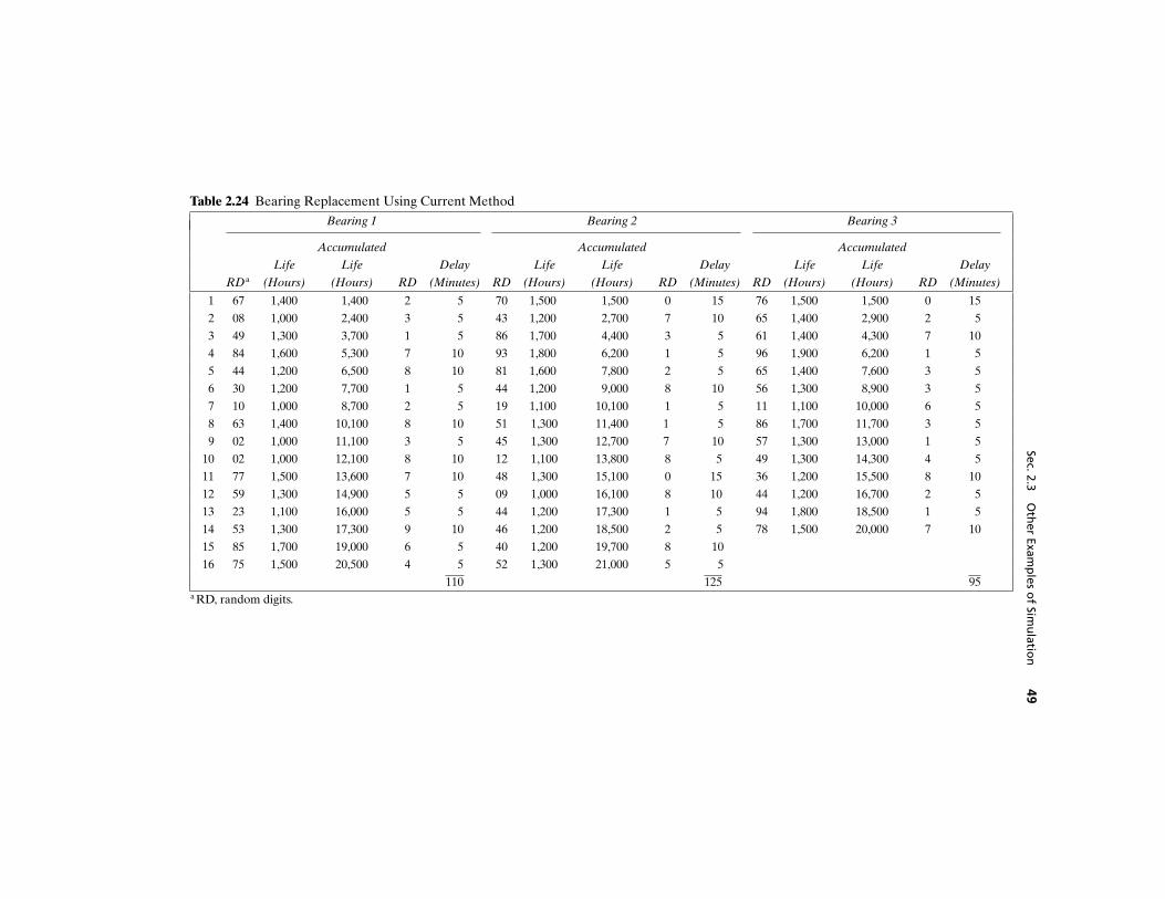
Sec.2.3O
ther
Examp
leso
fSim
ulatio
n49
Table 2.24 Bearing Replacement Using Current Method
Bearing 1 Bearing 2 Bearing 3
Accumulated Accumulated Accumulated
Life Life Delay Life Life Delay Life Life Delay
RDa (Hours) (Hours) RD (Minutes) RD (Hours) (Hours) RD (Minutes) RD (Hours) (Hours) RD (Minutes)
1 67 1,400 1,400 2 5 70 1,500 1,500 0 15 76 1,500 1,500 0 15
2 08 1,000 2,400 3 5 43 1,200 2,700 7 10 65 1,400 2,900 2 5
3 49 1,300 3,700 1 5 86 1,700 4,400 3 5 61 1,400 4,300 7 10
4 84 1,600 5,300 7 10 93 1,800 6,200 1 5 96 1,900 6,200 1 5
5 44 1,200 6,500 8 10 81 1,600 7,800 2 5 65 1,400 7,600 3 5
6 30 1,200 7,700 1 5 44 1,200 9,000 8 10 56 1,300 8,900 3 5
7 10 1,000 8,700 2 5 19 1,100 10,100 1 5 11 1,100 10,000 6 5
8 63 1,400 10,100 8 10 51 1,300 11,400 1 5 86 1,700 11,700 3 5
9 02 1,000 11,100 3 5 45 1,300 12,700 7 10 57 1,300 13,000 1 5
10 02 1,000 12,100 8 10 12 1,100 13,800 8 5 49 1,300 14,300 4 5
11 77 1,500 13,600 7 10 48 1,300 15,100 0 15 36 1,200 15,500 8 10
12 59 1,300 14,900 5 5 09 1,000 16,100 8 10 44 1,200 16,700 2 5
13 23 1,100 16,000 5 5 44 1,200 17,300 1 5 94 1,800 18,500 1 5
14 53 1,300 17,300 9 10 46 1,200 18,500 2 5 78 1,500 20,000 7 10
15 85 1,700 19,000 6 5 40 1,200 19,700 8 10
16 75 1,500 20,500 4 5 52 1,300 21,000 5 5
110 125 95a RD, random digits.
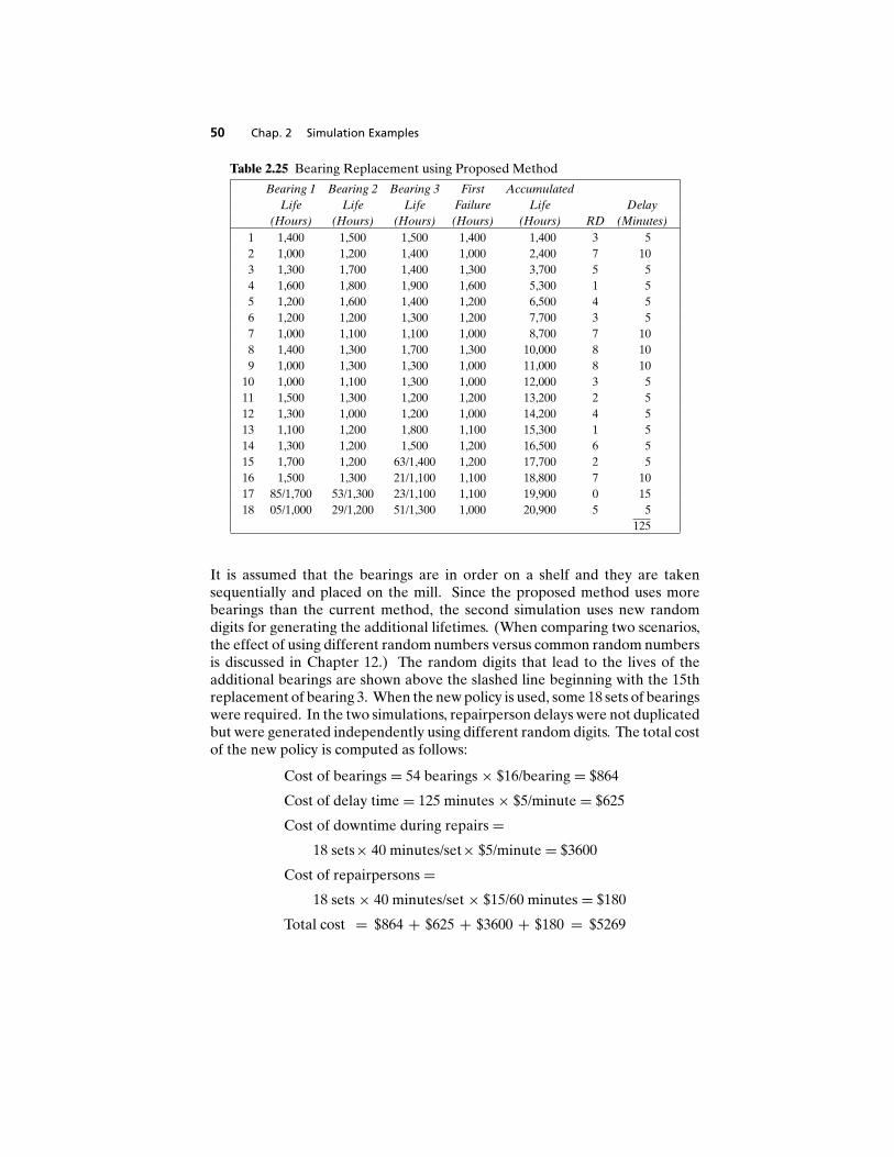
50 Chap. 2 Simulation Examples
Table 2.25 Bearing Replacement using Proposed Method
Bearing 1 Bearing 2 Bearing 3 First AccumulatedLife Life Life Failure Life Delay
(Hours) (Hours) (Hours) (Hours) (Hours) RD (Minutes)1 1,400 1,500 1,500 1,400 1,400 3 52 1,000 1,200 1,400 1,000 2,400 7 103 1,300 1,700 1,400 1,300 3,700 5 54 1,600 1,800 1,900 1,600 5,300 1 55 1,200 1,600 1,400 1,200 6,500 4 56 1,200 1,200 1,300 1,200 7,700 3 57 1,000 1,100 1,100 1,000 8,700 7 108 1,400 1,300 1,700 1,300 10,000 8 109 1,000 1,300 1,300 1,000 11,000 8 10
10 1,000 1,100 1,300 1,000 12,000 3 511 1,500 1,300 1,200 1,200 13,200 2 512 1,300 1,000 1,200 1,000 14,200 4 513 1,100 1,200 1,800 1,100 15,300 1 514 1,300 1,200 1,500 1,200 16,500 6 515 1,700 1,200 63/1,400 1,200 17,700 2 516 1,500 1,300 21/1,100 1,100 18,800 7 1017 85/1,700 53/1,300 23/1,100 1,100 19,900 0 1518 05/1,000 29/1,200 51/1,300 1,000 20,900 5 5
125
It is assumed that the bearings are in order on a shelf and they are takensequentially and placed on the mill. Since the proposed method uses morebearings than the current method, the second simulation uses new randomdigits for generating the additional lifetimes. (When comparing two scenarios,the effect of using different random numbers versus common random numbersis discussed in Chapter 12.) The random digits that lead to the lives of theadditional bearings are shown above the slashed line beginning with the 15threplacement of bearing 3. When the new policy is used, some 18 sets of bearingswere required. In the two simulations, repairperson delays were not duplicatedbut were generated independently using different random digits. The total costof the new policy is computed as follows:
Cost of bearings = 54 bearings × $16/bearing = $864
Cost of delay time = 125 minutes × $5/minute = $625
Cost of downtime during repairs =18 sets× 40 minutes/set× $5/minute = $3600
Cost of repairpersons =18 sets × 40 minutes/set × $15/60 minutes = $180
Total cost = $864 + $625 + $3600 + $180 = $5269
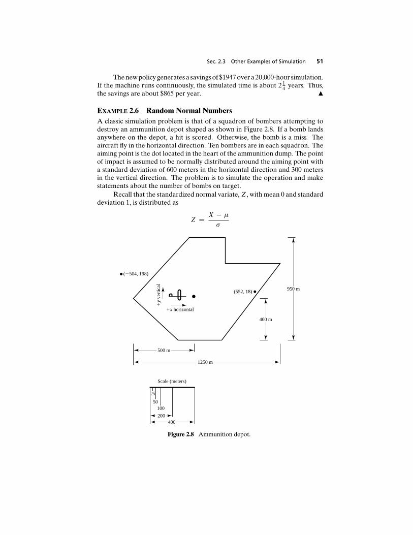
Sec. 2.3 Other Examples of Simulation 51
The new policy generates a savings of $1947 over a 20,000-hour simulation.If the machine runs continuously, the simulated time is about 2 1
4 years. Thus,the savings are about $865 per year. m
EXAMPLE 2.6 Random Normal NumbersA classic simulation problem is that of a squadron of bombers attempting todestroy an ammunition depot shaped as shown in Figure 2.8. If a bomb landsanywhere on the depot, a hit is scored. Otherwise, the bomb is a miss. Theaircraft fly in the horizontal direction. Ten bombers are in each squadron. Theaiming point is the dot located in the heart of the ammunition dump. The pointof impact is assumed to be normally distributed around the aiming point witha standard deviation of 600 meters in the horizontal direction and 300 metersin the vertical direction. The problem is to simulate the operation and makestatements about the number of bombs on target.
Recall that the standardized normal variate, Z , with mean 0 and standarddeviation 1, is distributed as
Z = X − µ
σ
500 m
1250 m
400 m
950 m
(2504, 198)
(552, 18)
1x horizontal
1y
vert
ical
400200
10050
25
Scale (meters)
Figure 2.8 Ammunition depot.

52 Chap. 2 Simulation Examples
where X is a normal random variable, µ is the true mean of the distribution ofX, and σ is the standard deviation of X. Then,
X = Zσ + µ.
In this example the aiming point can be considered as (0, 0); that is, the µ valuein the horizontal direction is 0, and similarly for the µ value in the verticaldirection. Then,
X = ZσX
Y = ZσY
where (X, Y ) are the simulated coordinates of the bomb after it has fallen.Now, σX = 600 and σY = 300. Therefore,
X = 600Zi
Y = 300Zj
The i and j subscripts have been added to indicate that the values of Z shouldbe different. What are these Z values and where can they be found? The valuesof Z are random normal numbers. These can be generated from uniformlydistributed random numbers, as discussed in Chapter 7. Alternatively, tablesof random normal numbers have been generated. A small sample of randomnormal numbers is given in Table A.2. If using a spreadsheet, there is a built-infunction that generates normal random numbers. (For Excel, use the RandomNumber Generation tool in the Analysis TookPak Add-In to generate anynumber of normal random values in a range of cells.)
To understand what happens in these bombing missions, a simulation ofperhaps 10 or 20 runs might be conducted. However, space limitations do notpermit such an extensive simulation. An example of one run will indicate howthe simulation is performed. The table of random normal numbers is used inthe same way as the table of random numbers: that is, start at a random placein the table and proceed in a systematic direction, avoiding overlap. Table 2.26shows the results of a simulated run.
The mnemonic RNNx stands for “random normal number to computethe x coordinate” and corresponds to Zi above. The first random normalnumber used was −0.84, generating an x coordinate 600(−0.84) = −504. Therandom normal number to generate the y coordinate was 0.66, resulting in a y
coordinate of 198. Taken together, (−504, 198) is a miss, for it is off the target.The resulting point and that of the third bomber are plotted on Figure 2.8. The10 bombers had 3 hits and 7 misses. Many more runs are needed to assess thepotential for destroying the dump. Additional runs appear as an exercise forthe reader. This is an example of a Monte Carlo, or static, simulation, sincetime is not an element of the solution. m

Sec. 2.3 Other Examples of Simulation 53
Table 2.26 Simulated Bombing Run
x Coordinate y Coordinate
Bomber RNNx (600 RNNx) RNNy (300 RNNy) Resulta
1 −0.84 −504 0.66 198 Miss
2 1.03 618 −0.13 −39 Miss
3 0.92 552 0.06 18 Hit
4 −1.82 −1,092 −1.40 −420 Miss
5 −0.16 −96 0.23 69 Hit
6 −1.78 −1,068 1.33 399 Miss
7 2.04 1,224 0.69 207 Miss
8 1.08 648 −1.10 −330 Miss
9 −1.50 −900 −0.72 −216 Miss
10 −0.42 −252 −0.60 −180 Hita Total: 3 hits, 7 misses.
EXAMPLE 2.7 Lead-Time Demand
Lead-time demand may occur in an inventory system when the lead time is otherthan instantaneous. The lead time is the time from placement of an order untilthe order is received. In a realistic situation, lead time is a random variable.During the lead time, demands also occur at random. Lead-time demand isthus a random variable defined as the sum of the demands over the lead time,or
∑Ti=0 Di , where i is the time period of the lead time, i = 0, 1, 2, . . . ; Di is
the demand during the i th time period; and T is the lead time. The distributionof lead-time demand is determined by simulating many cycles of lead time andbuilding a histogram based on the results.
A firm sells bulk rolls of newsprint. The daily demand is given by thefollowing probability distribution:
Daily Demand (Rolls) 3 4 5 6
Probability 0.20 0.35 0.30 0.15
The lead time is the number of days from placing an order until the firm receivesthe order from the supplier. In this instance, lead time is a random variablegiven by the following distribution:
Lead Time (Days) 1 2 3
Probability 0.36 0.42 0.22
Table 2.27 shows the random-digit assignment for demand, and Table 2.28does the same for lead time. The incomplete simulation table is shown inTable 2.29. The random digits for the first cycle were 57. This generates a leadtime of 2 days. Thus, two pairs of random digits must be generated for the
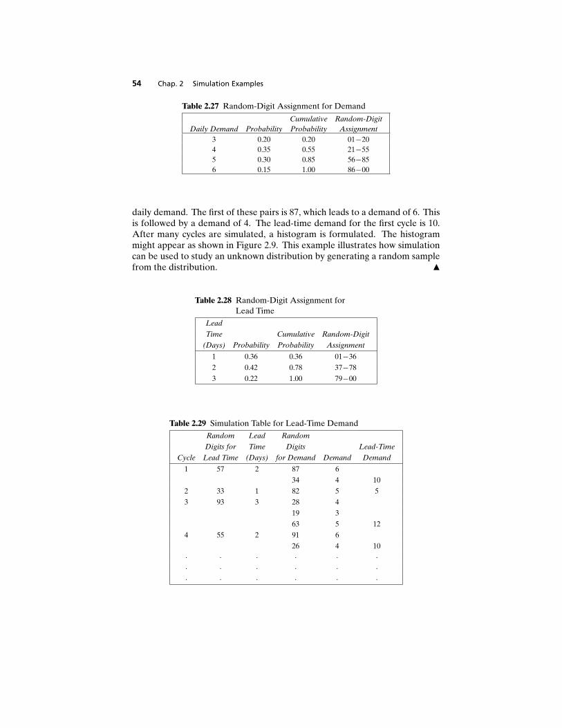
54 Chap. 2 Simulation Examples
Table 2.27 Random-Digit Assignment for Demand
Cumulative Random-DigitDaily Demand Probability Probability Assignment
3 0.20 0.20 01−204 0.35 0.55 21−555 0.30 0.85 56−856 0.15 1.00 86−00
daily demand. The first of these pairs is 87, which leads to a demand of 6. Thisis followed by a demand of 4. The lead-time demand for the first cycle is 10.After many cycles are simulated, a histogram is formulated. The histogrammight appear as shown in Figure 2.9. This example illustrates how simulationcan be used to study an unknown distribution by generating a random samplefrom the distribution. m
Table 2.28 Random-Digit Assignment forLead Time
Lead
Time Cumulative Random-Digit
(Days) Probability Probability Assignment
1 0.36 0.36 01−36
2 0.42 0.78 37−78
3 0.22 1.00 79−00
Table 2.29 Simulation Table for Lead-Time Demand
Random Lead Random
Digits for Time Digits Lead-Time
Cycle Lead Time (Days) for Demand Demand Demand
1 57 2 87 6
34 4 10
2 33 1 82 5 5
3 93 3 28 4
19 3
63 5 12
4 55 2 91 6
26 4 10
· · · · · ·· · · · · ·· · · · · ·
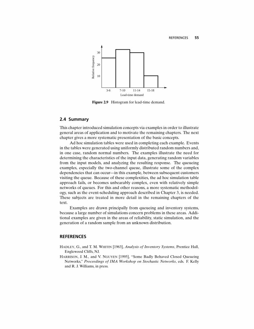
REFERENCES 55
10
20
30
Rel
ativ
e fr
eque
ncy
Lead-time demand
3-6 7-10 11-14 15-18
Figure 2.9 Histogram for lead-time demand.
2.4 Summary
This chapter introduced simulation concepts via examples in order to illustrategeneral areas of application and to motivate the remaining chapters. The nextchapter gives a more systematic presentation of the basic concepts.
Ad hoc simulation tables were used in completing each example. Eventsin the tables were generated using uniformly distributed random numbers and,in one case, random normal numbers. The examples illustrate the need fordetermining the characteristics of the input data, generating random variablesfrom the input models, and analyzing the resulting response. The queueingexamples, especially the two-channel queue, illustrate some of the complexdependencies that can occur—in this example, between subsequent customersvisiting the queue. Because of these complexities, the ad hoc simulation tableapproach fails, or becomes unbearably complex, even with relatively simplenetworks of queues. For this and other reasons, a more systematic methodol-ogy, such as the event-scheduling approach described in Chapter 3, is needed.These subjects are treated in more detail in the remaining chapters of thetext.
Examples are drawn principally from queueing and inventory systems,because a large number of simulations concern problems in these areas. Addi-tional examples are given in the areas of reliability, static simulation, and thegeneration of a random sample from an unknown distribution.
REFERENCES
HADLEY, G., and T. M. WHITIN [1963], Analysis of Inventory Systems, Prentice Hall,Englewood Cliffs, NJ.
HARRISON, J. M., and V. NGUYEN [1995], “Some Badly Behaved Closed QueueingNetworks,” Proceedings of IMA Workshop on Stochastic Networks, eds. F. Kellyand R. J. Williams, in press.
56 Chap. 2 Simulation Examples
EXERCISES
If solving a problem manually with a simulation table, use different random digitstaken from Table A.l for all problems referring to examples in the text. Many ofthe problems solved with a simulation table can be solved in a spreadsheet suchas Excel. If using a spreadsheet, the reader is encouraged to investigate in thehelp system the existence and syntax for some common but useful functions. [Forexample, in Excel, use RAND() for random numbers between 0 and 1; IF() toreturn one of two values depending on whether a condition is true or false; MAX()and MIN() for maximums and minimums, etc.] Recall, also, that numerous hintsfor spreadsheet implementation were given in the text for the queueing examples.
1 In Example 2.1, let the arrival distribution be uniformly distributed between 1 and10 minutes. Develop the simulation table and the analysis for 20 customers. Whatis the effect of changing the arrival-time distribution?
2 In Example 2.1, let the service distribution be changed to the following:
Service Time (Minutes) 1 2 3 4 5 6Probability 0.05 0.10 0.20 0.30 0.25 0.10
Develop the simulation table and the analysis for 20 customers. What is the effectof changing the service-time distribution?
3 Perform the simulation in Example 2.1 for 20 more customers (customers 21 through40). Compare the results of Example 2.1 to your results.
4 In Example 2.1, determine the time-weighted-average number of customers in thesystem and the time-weighted-average number of customers waiting. [Hint: UseFigure 2.6.]
5 In Example 2.2, change the arrival distribution of cars to the following:
Time betweenArrivals (Minutes) 0 1 2 3 4Probability 0.10 0.20 0.35 0.20 0.15
Develop the simulation and subsequent analysis for a period of 1 hour. What is theeffect of changing the arrival distribution?
6 Again, with respect to Example 2.2, Able has a kneecap injury and cannot moveas fast. Consequently, two things happen. Able’s service distribution changes andBaker gets first shot at the customer if both carhops are idle. Able’s new servicedistribution is as follows:
Service Time (Minutes) 3 4 5 6Probability 0.30 0.30 0.25 0.15
(a) Develop a simulation and subsequent analysis for 30 service completions.What is the effect of Able’s injury and the new rule?
(b) What would be the effect of adding a new employee who works at Baker’sspeed? The new employee would have all leftover work after Baker andAble.
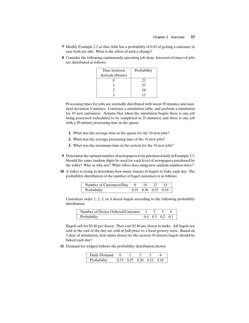
Chapter 2 Exercises 57
7 Modify Example 2.2 so that Able has a probability of 0.45 of getting a customer incase both are idle. What is the effect of such a change?
8 Consider the following continuously operating job shop. Interarrival times of jobsare distributed as follows:
Time between ProbabilityArrivals (Hours)
0 .231 .372 .283 .12
Processing times for jobs are normally distributed with mean 50 minutes and stan-dard deviation 8 minutes. Construct a simulation table, and perform a simulationfor 10 new customers. Assume that when the simulation begins there is one jobbeing processed (scheduled to be completed in 25 minutes) and there is one jobwith a 50-minute processing time in the queue.
1. What was the average time in the queue for the 10 new jobs?
2. What was the average processing time of the 10 new jobs?
3. What was the maximum time in the system for the 10 new jobs?
9 Determine the optimal number of newspapers to be purchased daily in Example 2.3.Should the same random digits be used for each level of newspapers purchased bythe seller? Why or why not? What effect does using new random numbers have?
10 A baker is trying to determine how many dozens of bagels to bake each day. Theprobability distribution of the number of bagel customers is as follows:
Number of Customers/Day 8 10 12 14Probability 0.35 0.30 0.25 0.10
Customers order 1, 2, 3, or 4 dozen bagels according to the following probabilitydistribution.
Number of Dozen Ordered/Customer 1 2 3 4Probability 0.4 0.3 0.2 0.1
Bagels sell for $5.40 per dozen. They cost $3.80 per dozen to make. All bagels notsold at the end of the day are sold at half-price to a local grocery store. Based on5 days of simulation, how many dozen (to the nearest 10 dozen) bagels should bebaked each day?
11 Demand for widgets follows the probability distribution shown:
Daily Demand 0 1 2 3 4Probability 0.33 0.25 0.20 0.12 0.10
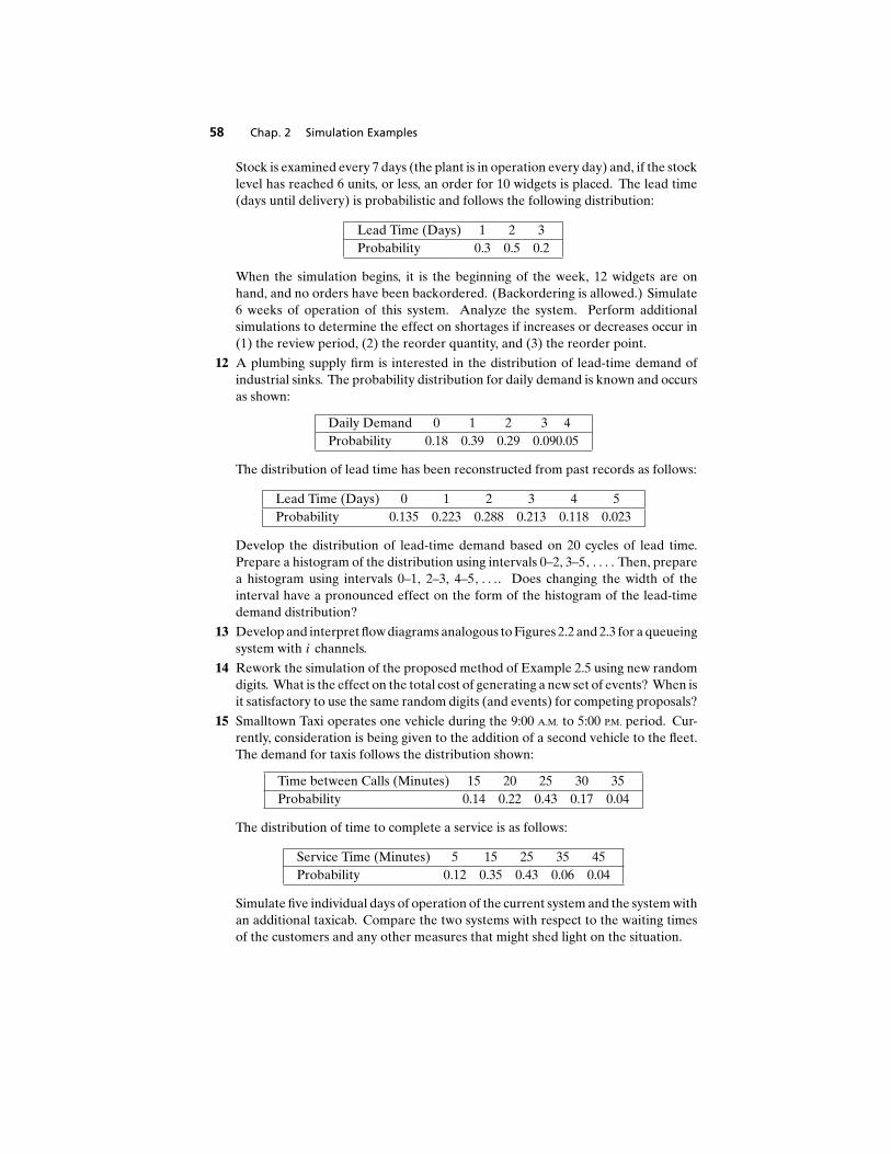
58 Chap. 2 Simulation Examples
Stock is examined every 7 days (the plant is in operation every day) and, if the stocklevel has reached 6 units, or less, an order for 10 widgets is placed. The lead time(days until delivery) is probabilistic and follows the following distribution:
Lead Time (Days) 1 2 3Probability 0.3 0.5 0.2
When the simulation begins, it is the beginning of the week, 12 widgets are onhand, and no orders have been backordered. (Backordering is allowed.) Simulate6 weeks of operation of this system. Analyze the system. Perform additionalsimulations to determine the effect on shortages if increases or decreases occur in(1) the review period, (2) the reorder quantity, and (3) the reorder point.
12 A plumbing supply firm is interested in the distribution of lead-time demand ofindustrial sinks. The probability distribution for daily demand is known and occursas shown:
Daily Demand 0 1 2 3 4Probability 0.18 0.39 0.29 0.090.05
The distribution of lead time has been reconstructed from past records as follows:
Lead Time (Days) 0 1 2 3 4 5Probability 0.135 0.223 0.288 0.213 0.118 0.023
Develop the distribution of lead-time demand based on 20 cycles of lead time.Prepare a histogram of the distribution using intervals 0–2, 3–5, . . . . Then, preparea histogram using intervals 0–1, 2–3, 4–5, . . .. Does changing the width of theinterval have a pronounced effect on the form of the histogram of the lead-timedemand distribution?
13 Develop and interpret flow diagrams analogous to Figures 2.2 and 2.3 for a queueingsystem with i channels.
14 Rework the simulation of the proposed method of Example 2.5 using new randomdigits. What is the effect on the total cost of generating a new set of events? When isit satisfactory to use the same random digits (and events) for competing proposals?
15 Smalltown Taxi operates one vehicle during the 9:00 A.M. to 5:00 P.M. period. Cur-rently, consideration is being given to the addition of a second vehicle to the fleet.The demand for taxis follows the distribution shown:
Time between Calls (Minutes) 15 20 25 30 35Probability 0.14 0.22 0.43 0.17 0.04
The distribution of time to complete a service is as follows:
Service Time (Minutes) 5 15 25 35 45Probability 0.12 0.35 0.43 0.06 0.04
Simulate five individual days of operation of the current system and the system withan additional taxicab. Compare the two systems with respect to the waiting timesof the customers and any other measures that might shed light on the situation.

Chapter 2 Exercises 59
16 Continue Example 2.6 for nine more runs and estimate how well the simulatedbombers will do when they make their raid on the ammunition depot.
17 The random variables X, Y , and Z are distributed as follows:
X ∼ N(µ = 100, σ 2 = 100)
Y ∼ N(µ = 300, σ 2 = 225)
Z ∼ N(µ = 40, σ 2 = 64)
Simulate 50 values of the random variable
W = X + Y
Z
Prepare a histogram of the resulting values using class intervals of width equal to3.
18 Given A, B , and C , three independent random variables: Variable A is normallydistributed with µ = 100 and σ 2 = 400. Variable B is discrete uniformly dis-tributed with probability distribution given by p(b) = 1/5 with b = 0, 1, 2, 3 and4. Variable C is distributed in accordance with the following table.
Value of C Probability10 .1020 .2530 .5040 .15
Use simulation to estimate the mean of a new variable D , defined as
D = (A − 25B)/(2C)
Use a sample of size 10.
19 Lead time for a stock item is normally distributed with a mean of 7 days and astandard deviation of 2 days. Daily demand is distributed as follows:
Daily Demand 0 1 2 3 4Probability 0.367 0.368 0.184 0.062 0.019
Determine the lead-time demand for 20 order cycles. (Round off lead time to theclosest integer during the simulation and, if a negative value results, give it a leadtime of zero.)
20 Consider Example 2.4.
(a) Extend the example for 15 more cycles and draw conclusions.
(b) Rework the example for 10 cycles with M = 10.
(c) Rework the example for 10 cycles with N = 6.

60 Chap. 2 Simulation Examples
21 Estimate, by simulation, the average number of lost sales per week for an inventorysystem that functions as follows:
(a) Whenever the inventory level falls to or below 10 units, an order is placed.Only one order can be outstanding at a time.
(b) The size of each order is equal to 20 − I , where I is the inventory level whenthe order is placed.
(c) If a demand occurs during a period when the inventory level is zero, the saleis lost.
(d) Daily demand is normally distributed with a mean of 5 units and a standarddeviation of 1.5 units. (Round off demands to the closest integer during thesimulation and, if a negative value results, give it a demand of zero.)
(e) Lead time is distributed uniformly between zero and 5 days, integers only.
(f) The simulation will start with 18 units in inventory.
(g) For simplicity, assume that all demands occur at 12 noon and that all ordersare placed at the same time. Assume further that orders are received at 5:00P.M., or after the demand which occurred on that day.
(h) Let the simulation run for 5 weeks.
22 An elevator in a manufacturing plant carries exactly 400 kilograms of material.There are three kinds of material, which arrive in boxes of known weight. Thesematerials and their distributions of time between arrivals are as follows:
Material Weight (kilograms) Interarrival Time (Minutes)A 200 5 ± 2(uniform)B 100 6(constant)C 50 P(2) = 0.33
P(3) = 0.67
It takes the elevator 1 minute to go up to the second floor, 2 minutes to unload, and1 minute to return to the first floor. The elevator does not leave the first floor unlessit has a full load. Simulate 1 hour of operation of the system. What is the averagetransit time for a box of material A (time from its arrival until it is unloaded)? Whatis the average waiting time for a box of material B? How many boxes of materialC made the trip in 1 hour?
23 The random variables X and Y are distributed as follows:
X ∼ 10 ± 10 (uniform)
Y ∼ 10 ± 8 (uniform)
(a) Simulate 200 values of the random variable
Z = XY
Prepare a histogram of the resulting values. What is the range of Z and whatis its average value?
(b) Same as (a) exceptZ = X/Y
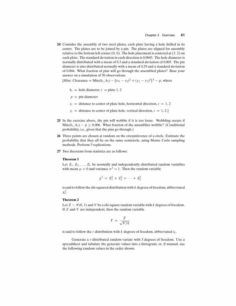
Chapter 2 Exercises 61
24 Consider the assembly of two steel plates, each plate having a hole drilled in itscenter. The plates are to be joined by a pin. The plates are aligned for assemblyrelative to the bottom left corner (0, 0). The hole placement is centered at (3, 2) oneach plate. The standard deviation in each direction is 0.0045. The hole diameter isnormally distributed with a mean of 0.3 and a standard deviation of 0.005. The pindiameter is also distributed normally with a mean of 0.29 and a standard deviationof 0.004. What fraction of pins will go through the assembled plates? Base youranswer on a simulation of 50 observations.
[Hint: Clearance = Min(h1, h2) − [(x1 − x2)2 + (y 1 − y 2)
2].5 − p , where
hi = hole diameter, i = plate 1, 2
p = pin diameter
xi = distance to center of plate hole, horizontal direction, i = 1, 2
yi = distance to center of plate hole, vertical direction, i = 1, 2.]
25 In the exercise above, the pin will wobble if it is too loose. Wobbling occurs ifMin(h1, h2) − p ≥ 0.006. What fraction of the assemblies wobble? (Conditionalprobability, i.e., given that the pins go through.)
26 Three points are chosen at random on the circumference of a circle. Estimate theprobability that they all lie on the same semicircle, using Monte Carlo samplingmethods. Perform 5 replications.
27 Two theorems from statistics are as follows:
Theorem 1
Let Z1, Z2, . . . , Zk be normally and independently distributed random variableswith mean µ = 0 and variance σ 2 = 1. Then the random variable
χ2 = Z21 + Z2
2 + · · · + Z2k
is said to follow the chi-squared distribution with k degrees of freedom, abbreviatedχ2
k .
Theorem 2
Let Z ∼ N(0, 1) and V be a chi-square random variable with k degrees of freedom.If Z and V are independent, then the random variable
T = Z√V/k
is said to follow the t distribution with k degrees of freedom, abbreviated tk .
Generate a t -distributed random variate with 3 degrees of freedom. Use aspreadsheet and tabulate the generate values into a histogram; or, if manual, usethe following random values in the order shown:
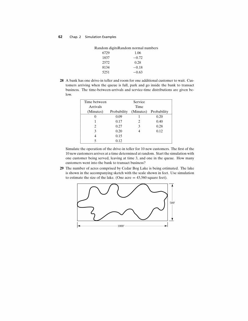
62 Chap. 2 Simulation Examples
Random digitsRandom normal numbers6729 1.061837 −0.722572 0.288134 −0.185251 −0.63
28 A bank has one drive-in teller and room for one additional customer to wait. Cus-tomers arriving when the queue is full, park and go inside the bank to transactbusiness. The time-between-arrivals and service-time distributions are given be-low.
Time between ServiceArrivals Time
(Minutes) Probability (Minutes) Probability0 0.09 1 0.201 0.17 2 0.402 0.27 3 0.283 0.20 4 0.124 0.155 0.12
Simulate the operation of the drive-in teller for 10 new customers. The first of the10 new customers arrives at a time determined at random. Start the simulation withone customer being served, leaving at time 3, and one in the queue. How manycustomers went into the bank to transact business?
29 The number of acres comprised by Cedar Bog Lake is being estimated. The lakeis shown in the accompanying sketch with the scale shown in feet. Use simulationto estimate the size of the lake. (One acre = 43,560 square feet).
1000'
500'


