Introduction to Geometric Mechanics

and AVI

Francois Demoures

Tudor Ratiu, Yves Weinand

CAG, IBOIS, EPFL

francois.demoures@epfl.ch

MIT - Prof Radovitzky, May 13, 2010

1

Plan of presentation

• Continuous mechanics

• Discrete mechanics

• Asynchronous Variational Integrator

MIT - Prof Radovitzky, May 13, 2010

2

Continuous mechanics

MIT - Prof Radovitzky, May 13, 2010

3

References for continuous mechanics

Ralph Abraham, Jerrold E. Marsden [1987], Foundations of Me-

chanics. Addison-Wesley Publishing Company, Inc.

Ralph Abraham, Jerrold E. Marsden, Tudor S. Ratiu [1991], Mani-

folds, Tensor Analysis, and Applications. Springer

Jerrold E. Marsden, Tudor S. Ratiu [1999], Introduction to Me-

chanics and Symmetry. Springer

MIT - Prof Radovitzky, May 13, 2010

4

Continuous mechanics

• a) Differentiable manifold and tangent bundle

• b) Lagrangian mechanics

• c) Hamiltonian mechanics

• d) Lie group and Lie algebra

• e) Symplectic property and Noether’s theorem

5

Differentiable manifold. The basic idea of a manifold is to intro-duce a local object that will support differentiation process.

Let S a set, and U ⊂ S with a one-to-one mapping φ : U → F

as a chart (U, φ) or coordinate system xi, where xi denote thecomponents of this mapping. Where F is a subset of a Banachspace, as Rn.

For two charts (Ui, φi), (Uj, φj) and φi∩φj 6= ∅ let the overlap mapφji = φj φ−1

i : φi(Ui ∩ Uj)→ φj(Ui ∩ Uj).

An atlas A on S is a family of charts such that S =⋃i∈I Ui, and

overlap maps φji are C∞ diffeomorphisms.

Ui

Uj

S

φi

φj

φji Rn

6

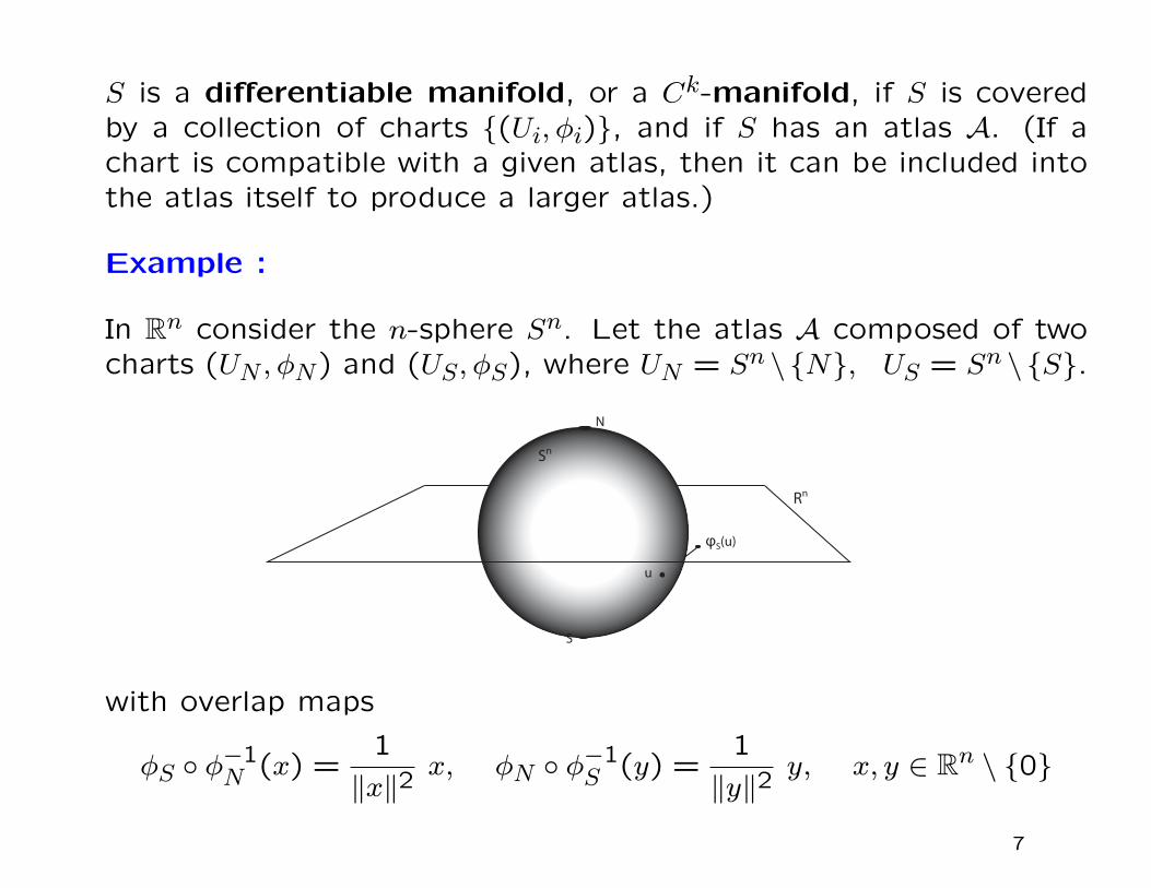
S is a differentiable manifold, or a Ck-manifold, if S is coveredby a collection of charts (Ui, φi), and if S has an atlas A. (If achart is compatible with a given atlas, then it can be included intothe atlas itself to produce a larger atlas.)

Example :

In Rn consider the n-sphere Sn. Let the atlas A composed of twocharts (UN , φN) and (US, φS), where UN = Sn \N, US = Sn \S.

φN(u)

φS(u)

u

N

S

Sn

Rn

with overlap maps

φS φ−1N (x) =

1

‖x‖2x, φN φ−1

S (y) =1

‖y‖2y, x, y ∈ Rn \ 0

7

Tangent bundle.

Let M a differentiable n-manifold with local coordinate xi, the

tangent bundle of M , denoted by TM , is the set of the tangent

space to M at the points m ∈M , that is

TM =⋃

m∈MTmM.

TM is a 2n-manifold, with local coordinate xi, vi, where vi is a

tangent vector.

The natural projection is the map

τM : TM →M, v 7→ m

where v is the vector attached to the point m. And the inverse

image τ−1M (m) is the fiber of the tangent bundle over the point

m ∈M .

8

Lagrangian mechanics.

Configuration space Q as a manifold, is the set of all possible

spatial positions of bodies in the system. Given a time interval [0, T ]

define the path space to be C(Q) = q : [0, T ]→ Q | q ∈ C2([0, T ]),which is a C∞-manifold.

The collection of pairs (q, q) as elements of the tangent bundle TqQ,

also called velocity phase space, with basis ∂/∂q1, ..., ∂/∂qn.

The Lagrangian L(qi, qi) : TQ→ R is often seen as the kinetic en-

ergy minus the potential energy, where (q1, ..., qn) are configurations

coordinates.

Given a time interval [0, T ], let the action map G : C(Q)→ R

G(q) =∫ T

0L(qi(t), qi(t))dt.

9

Hamilton’s principle or principle of critical action, seeks curves

q(t) for which the action map G is stationary under variations of

q(t) with fixed endpoints : δqi(0) = δqi(T ) = 0, and time interval.

δG(q) =∫ T

0

(∂L

∂qiδqi +

∂L

∂qiδqi)dt =

∫ T0

(∂L

∂qiδqi −

d

dt

∂L

∂qiδqi)dt = 0

q(0)

q(T )

δq(t)

Q

q(t) varied curve

gives the well-known Euler-Lagrange equations :

∂L

∂qi−d

dt

∂L

∂qi= 0

10

Example : For a system of N particles∗ moving in Euclidean 3-

space, we choose the configuration space to be Q = R3× ...×R3 =

R3N , and

L(qj, qj) =1

2

N∑j=1

mj‖qj‖2 − V (qj), qj ∈ R3

Where 12mj||qj||2 is the kinetic energy, and V (qj) is the potential

energy of the particle j.

The Euler-Lagrange equations are

d

dt

(mj qj

)= −

∂V

∂qj, j = 1, ..., N.

∗Newton’s second law for a particle qj moving in Euclidean three-space R3

under the influence of a potential energy V (qj) is : mqj = −∇V (qj)

11

Hamiltonian mechanics.

Motivation : For a particle q, let E the total energy, such that

dE/dt = 0, as

E(q) =1

2m||q||2 + V (q)

Lagrange and Hamilton observed that it is convenient to introduce

the momentum pi = mqi and rewrite E as

H(q,p) =||p||2

2m+ V (q)

for then Newton’s second law is equivalent to Hamilton’s canon-

ical equations

qi =∂H

∂pi, pi = −

∂H

∂qi

where (q,p) is phase space.

12

Let a manifold M , the cotangent bundle T ∗M , or the dual of TM ,

is the space of differential df , for all smooth function f : M → R.

df(x) =∂f

∂xidxi

The cotangent bundle T ∗Q of the configuration space Q is the space

where (dq1, ..., dqn).

Define the fiber derivative or Legendre transform FL : TQ→ T ∗Qby

FL(v).w =d

ds

∣∣∣∣s=0

L(v + sw), v, w ∈ TqQ

which is the derivative of Lagrangian L at v along the fiber TqQ

in the direction w. So, for finite-dimensional manifold and (qi, qi)

coordinates on TqQ, we get

FL(qi, qi) =

(qi,

∂L

∂qi

)= (qi, pi) ∈ T ∗qQ,

where pi is the conjugate momenta which is not always mq.

13

If the fiber derivative FL is locally an isomorphism then we say thatL is regular.

Assume that Legendre transform is invertible and define the Hamil-

tonian H : T ∗Q→ R by

H(qi, pi) = piqi − L(qi, qi),

then the Euler-Lagrange equations are equivalent to Hamilton’s

equations

qi =∂H

∂pi, pi = −

∂H

∂qi, i = 1, ..., n.

Which can be view as follows(∂H

∂pi,−∂H

∂qi

)= (qi, pi)

where XH(z) =:

(∂H

∂pi,−∂H

∂qi

)=

[0 I−I 0

]dH(z)

is the Hamiltonian vector field, and (q(t),p(t)) is an integral curveof XH.

14

Example : simple pendulum. Lagrangian and Hamiltonian pointof view.

θ

l

x2

x3

X

x1

The configuration space is the sphere S2l of radii l

Q = S2l ,

x1 = 0

x2 = lsin(θ)x3 = lcos(θ)

x1 = 0

x2 = lθcos(θ)x3 = −lθsin(θ)

And, for Euclidean metric tensor gij, the Lagrangian L(θ, θ) is

L(θ, θ) =1

2m

3∑i,j=1

gijxixj − V (θ) =

1

2m(lθ)2

+mg (lcos(θ))

Euler-Lagrange equation gives the equation of the motion

d

dt

(∂L

∂θ

)−∂L

∂θ= ml2θ +mglsin(θ) = 0

15

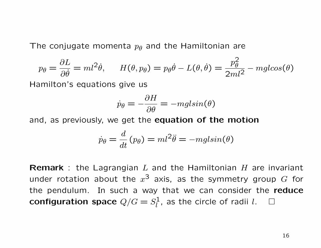
The conjugate momenta pθ and the Hamiltonian are

pθ =∂L

∂θ= ml2θ, H(θ, pθ) = pθθ − L(θ, θ) =

p2θ

2ml2−mglcos(θ)

Hamilton’s equations give us

pθ = −∂H

∂θ= −mglsin(θ)

and, as previously, we get the equation of the motion

pθ =d

dt(pθ) = ml2θ = −mglsin(θ)

Remark : the Lagrangian L and the Hamiltonian H are invariant

under rotation about the x3 axis, as the symmetry group G for

the pendulum. In such a way that we can consider the reduce

configuration space Q/G = S1l , as the circle of radii l.

16

Symplectic property. Motivation :

Let a given region of initial conditions in phase-space (qi, pi) ∈T ∗qQ. When the phenomenon is symplectic, if we advance all statessimultaneously, regions of phase space, are deformed under the flow,in a way that preserves the original area, as on the right figure.

The pendulum: in this example three integrators behave very dif-ferently motion of a pendulum: while on the left it amplifies oscil-lations, and in the middle it dampens the motion, on the right thesymplectic integrator captures the periodic nature of the pendulum.

17

Let the Hamiltonian vector field XH : T ∗Q → T (T ∗Q), as define

XH(z) :=(∂H∂pi,−∂H

∂qi

). And the Hamiltonian flow F tH(z) which is

the integral curve of XH(z).

Hamiltonian flows are symplectic. Formally, this means that the

flow preserves the canonical symplectic Hamiltonian two-form

ΩH = dqi ∧ dpi. Which means F ∗HΩH = ΩH.

In the same way Lagrangian flows F tL (i.e., motions) are sym-

plectic. Such as, if the Lagrangian is regular we can define FLlocally, as

FL = FL−1 FH FL.

Remark : The symplectic form ΩH = dqi∧dpi defines the geometry

of a symplectic manifold (T ∗Q,ΩH), much as the metric tensor

defines the geometry of a Riemannian manifold.

18

Lie group and Lie algebra.

A Lie group is a manifold G that has a group structure (G,µ) con-

sistent with its manifold structure in the sense that group operation

µ : G×G→ G, (g, h) 7→ µ(g, h)

is a C∞ map.

Examples : a) Any Banach space F , admits an atlas formed by the

single chart identity, and is an Abelian Lie group with + operation.

We call such a group a vector group. (For example, the space

L(Rn,Rn) of all continuous linear maps of Rn to Rn is a Banach

space and a vector group.)

b) The orthogonal group O(n) = A ∈ GL(n,R)| AAT = 1, as

a closed Lie subgroup of the Lie group GL(n,R) of linear isomor-

phisms of Rn to Rn, is a Lie group with group operation µ(A,B) =

A B.

19

Let G a Lie group, the vector space TeG, as tangent vector to G

at the identity e ∈ G, with Lie algebra structure (TeG,+, · , [ , ]) is

called the Lie algebra of G, and is denoted by g. Where [ , ] is the

Lie bracket in TeG.

Examples : a) For a Banach space F , the Lie algebra is itself, with

the trivial bracket [v, w] = 0 for all v, w ∈ F .

b) The Lie algebra of GL(n,R) is L(Rn,Rn), also denoted gl(n),

with the bracket

[v, w] = vw − wv

c) The Lie algebra so(3) of the Lie group SO(3) is

so(3) = v : R3 → R3| v + vT = 0

with the same bracket as for gl(n).

20

Example of Lie group and Lie algebra application : thin-shell

model of Simo and Fox.∗

Let the differentiable manifold

C := (ϕ, t)| A ⊂ R2 → R3 × S2

where A is an open set with smooth boundary ∂A, and compact

closure A. Any configuration of the shell is assumed to be defined

by a pair (ϕ, t) ∈ C as

S := x ∈ R3| x = ϕ+ ξt, where (ϕ, t) ∈ C, ξ ∈[h−, h+

]

where the map ϕ : A → R3 defines the position of the mid-surface

of the shell, and the map t : A → S2 defines a unit vector field as

the director field.

∗J.C. Simo, D.D. Fox [1989], On a stress resultant geometrically exact shellmodel. Part I : Formulation and optimal parameterization. Comput. MethodsAppl. Mech. Engrg. 72(3), 267-304.

21

Let Eii=1,2,3 an orthonormal basis as the standard basis. Then t

may be defined as t = ΛE3, where Λ ∈ S2E3

, a SO(3) Lie subgroup.

S2E3

:= Λ ∈ SO(3)| ∀Ψ ∈ R3 such that ΛΨ = Ψ, then < Ψ,E3 >= 0

And the time differentiation of the director t is

t = ΛE = ΛWE

where t ∈ TS2, and W ∈ T1S2E3⊂ so(3), where W represents an

infinitesimal rotation about W ∈ R3 define as follows :

so(3) may be identified with R3 by the isomorphism

: R3 → so(3), W = (W1,W2,W3) 7→ W =

0 −W3 W2W3 0 −W1−W2 W1 0

with the identity WV = W ×V, for all V ∈ R3.

22

Hamiltonian Noether’s theorem. When the Lie group action

is a symmetry group of the Hamiltonian, then the corresponding

Hamiltonian momentum maps J : T ∗Q → g∗ are preserved by the

Hamiltonian flow φt, that is J φt = J.

We have an equivalent Lagrangian form of Noether’s theorem.

Examples : a) Linear momentum. Let the N-particles system

and consider the translation on every factor, or R3-action on R3N .

The total linear momentum of the N-particle system is

J(qj,pj) =

N∑j=1

pj

Given a Hamiltonian H, determining the evolution of the N-particle

system, Noether’s theorem establish that the total linear momen-

tum J is conserved if H is translation-invariant.

23

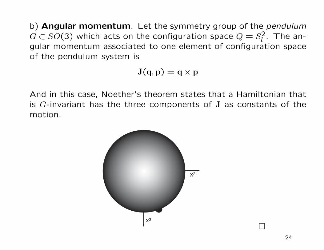
b) Angular momentum. Let the symmetry group of the pendulumG ⊂ SO(3) which acts on the configuration space Q = S2

l . The an-gular momentum associated to one element of configuration spaceof the pendulum system is

J(q,p) = q× p

And in this case, Noether’s theorem states that a Hamiltonian thatis G-invariant has the three components of J as constants of themotion.

θ

l

x2

x3

X

x1

24

Discrete mechanics

MIT - Prof Radovitzky, May 13, 2010

25

References for discrete mechanics

Jerrold E. Marsden, M. West [2001], Discrete mechanics and vari-

ational integrators. Cambridge University Press

Melvin Leok [2004], Foundations of computational geometric me-

chanics. Thesis - Caltech

M. West [2004], Variational integrators. Thesis - Caltech

MIT - Prof Radovitzky, May 13, 2010

26

Discrete mechanics

• a) Discrete variational mechanics

• b) Hamiltonian viewpoint

• c) One-step integrator and its properties

• d) Non-holonomic constraint

27

Discrete variational mechanics. Let a configuration manifold Q,

as previously, but now define the discrete state space to be Q×Q(which contains the same amount of information as TQ).

To relate discrete to continuous mechanics, we introduce sequence

of time tk = kh | k = 0, ..., N, where h ∈ R is a discrete time

step.

We can define the discrete path space Cd(Q) = qd : tkNk=0 →Q = qkNk=0, which is isomorphic to R × ... × R, (N + 1 copies),

where qk = q(tk).

The discrete action map Sd : Cd(Q)→ R is defined by

Sd(qd) =N−1∑k=0

Ld(qk, qk+1).

28

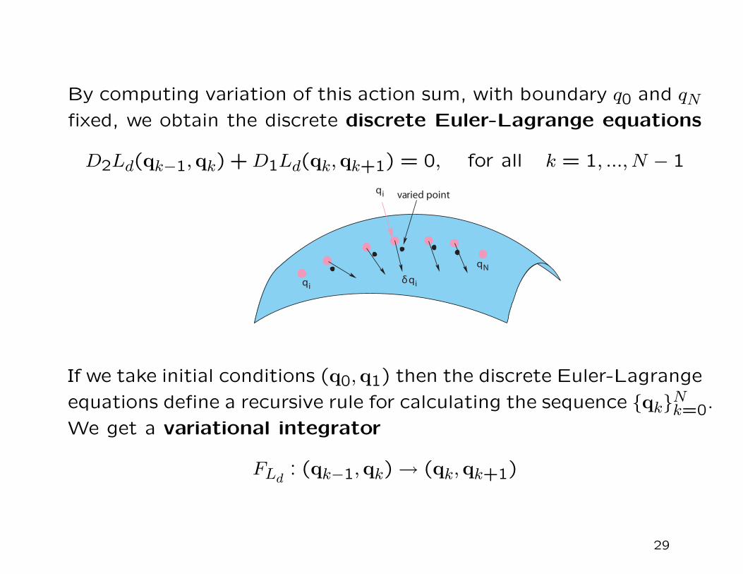
By computing variation of this action sum, with boundary q0 and qNfixed, we obtain the discrete discrete Euler-Lagrange equations

D2Ld(qk−1,qk) +D1Ld(qk,qk+1) = 0, for all k = 1, ..., N − 1

qi

qNδqi

qi varied point

If we take initial conditions (q0,q1) then the discrete Euler-Lagrange

equations define a recursive rule for calculating the sequence qkNk=0.

We get a variational integrator

FLd : (qk−1,qk)→ (qk,qk+1)

29

Ld : Q×Q→ R is a discrete Lagrangian of order r, if it satisfies

Ld(qk,qk+1,∆t) =∫ tk+1

tkL(q, q)dt+O(∆t)r+1,

where L is the Lagrangian of the continuous systems and q(t) isthe solution of the Euler-Lagrange equations satisfying q(tk) = qkand q(tk+1) = qk+1.

Example : If we take, as discrete Lagrangian

Lαd(qk,qk+1, h) = hL

((1− α)qk + αqk+1,

qk+1 − qkh

),

variational integrator is explicit for α = 0 or α = 1, but only firstorder. And is second order if and only if α = 1/2, but in this casevariational integrator is implicit.

An interesting choice of discrete Lagrangian is Lagrangian as kineticenergy minus potential energy, with α = 0, to get explicit integrator

Ld(qk,qk+1, h) =h

2

(qk+1 − qk

h

)TM

(qk+1 − qk

h

)− hV (qk).

30

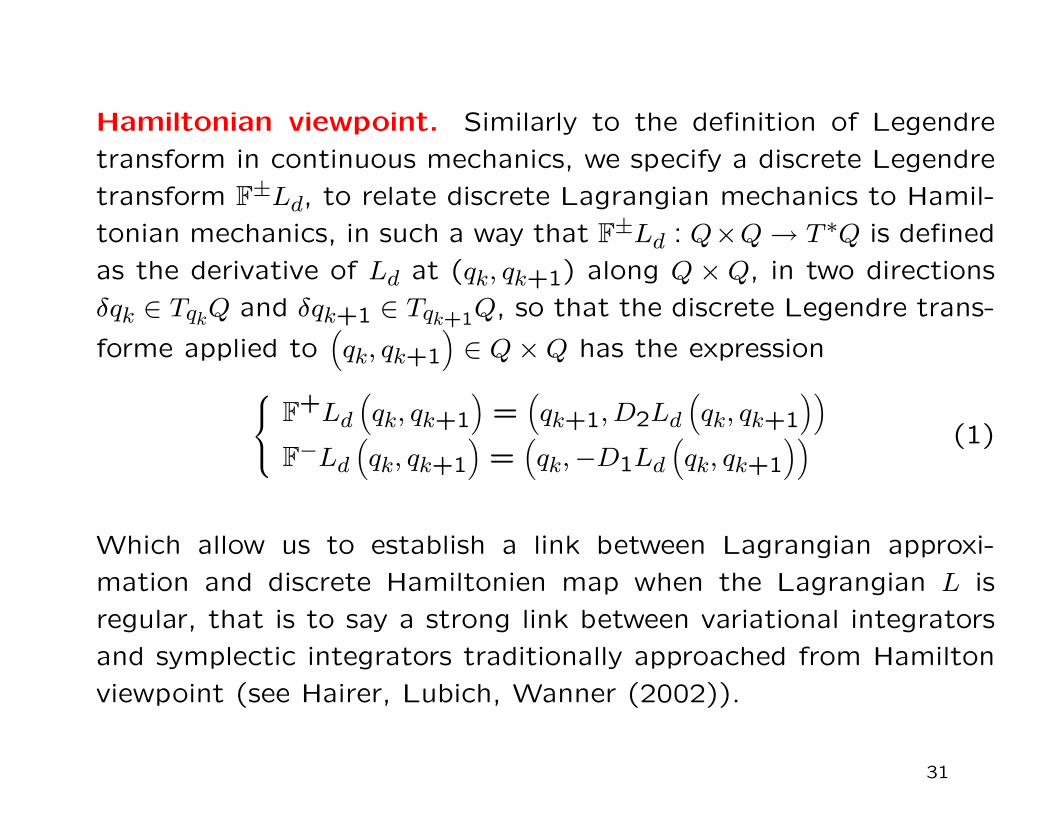
Hamiltonian viewpoint. Similarly to the definition of Legendre

transform in continuous mechanics, we specify a discrete Legendre

transform F±Ld, to relate discrete Lagrangian mechanics to Hamil-

tonian mechanics, in such a way that F±Ld : Q×Q→ T ∗Q is defined

as the derivative of Ld at (qk, qk+1) along Q×Q, in two directions

δqk ∈ TqkQ and δqk+1 ∈ Tqk+1Q, so that the discrete Legendre trans-

forme applied to(qk, qk+1

)∈ Q×Q has the expression F+Ld

(qk, qk+1

)=(qk+1, D2Ld

(qk, qk+1

))F−Ld

(qk, qk+1

)=(qk,−D1Ld

(qk, qk+1

)) (1)

Which allow us to establish a link between Lagrangian approxi-

mation and discrete Hamiltonien map when the Lagrangian L is

regular, that is to say a strong link between variational integrators

and symplectic integrators traditionally approached from Hamilton

viewpoint (see Hairer, Lubich, Wanner (2002)).

31

Properties of one-step integrator : FLd : (xk−1, xk) 7→ (xk, xk+1)

It has two important structure preserving properties, as in continu-

ous mechanics :

• First, FLd is symplectic which implies area preservation in phase-

space or, more precisely,(FLd

)∗ΩLd

= ΩLd, where ΩLd

is a discrete

Lagrangian 2-form.

• Secondly, if discrete Lagrangian Ld inherits the same symmetry

groups as the continuous system, which means it is invariant under

a Lie group action, then the discrete Lagrangian momentum

map JLd is a conserved quantity : JLd FLd = JLd.

32

Non-holonomic constraint. Given discrete Lagrangian forces

(which are fibre-preserving), we modify the discrete Hamiltons prin-

ciple to the discrete Lagrange-d’Alembert principle which states

that the discrete trajectory qk, with prescribed initial and final

endpoints, satisfy

δN∑k=0

Ld(qk, qk+1) +N∑k=0

[f−d (qk, qk+1)δqk + f+

d (qk, qk+1)δqk+1

]= 0

where f−d and f+d are left and right discrete Lagrangian forces. And

we get the forced discrete Euler-Lagrange equations

D2Ld(qk−1, qk

)+D1Ld

(qk, qk+1

)+ f+

d

(qk−1, qk

)+ f−d

(qk, qk+1

)= 0,

The forced discrete Lagrangian flow FLd : Q×Q→ Q×Q, we get,

is a one-step integrator, which conserve momentums associated to

symmetries.

33

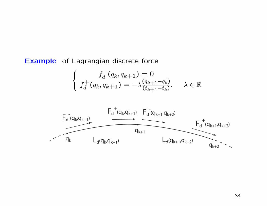
Example of Lagrangian discrete force f−d (qk, qk+1) = 0

f+d (qk, qk+1) = −λ(qk+1−qk)

(tk+1−tk) , λ ∈ R

Fd-(qk,qk+1)

Fd+

(qk,qk+1) Fd-(qk+1,qk+2)

Fd+

(qk+1,qk+2)

Ld(qk,qk+1) Ld(qk+1,qk+2)qk

qk+1

qk+2

34

AVI

MIT - Prof Radovitzky, May 13, 2010

35

References for AVI

A. Lew, J. E. Marsden, M. Ortiz, and M. West - Variational time

integrators - International journal for numerical methods in engi-

neering. 2003

J.E. Marsden, and M. West - Discrete mechanics and variational

integrators - Cambridge University Press - 2001

MIT - Prof Radovitzky, May 13, 2010

36

AVI

• a) AVI and energy conservation.

• b) Convergence

• c) Simplicity and Noether’s theorem for AVI

37

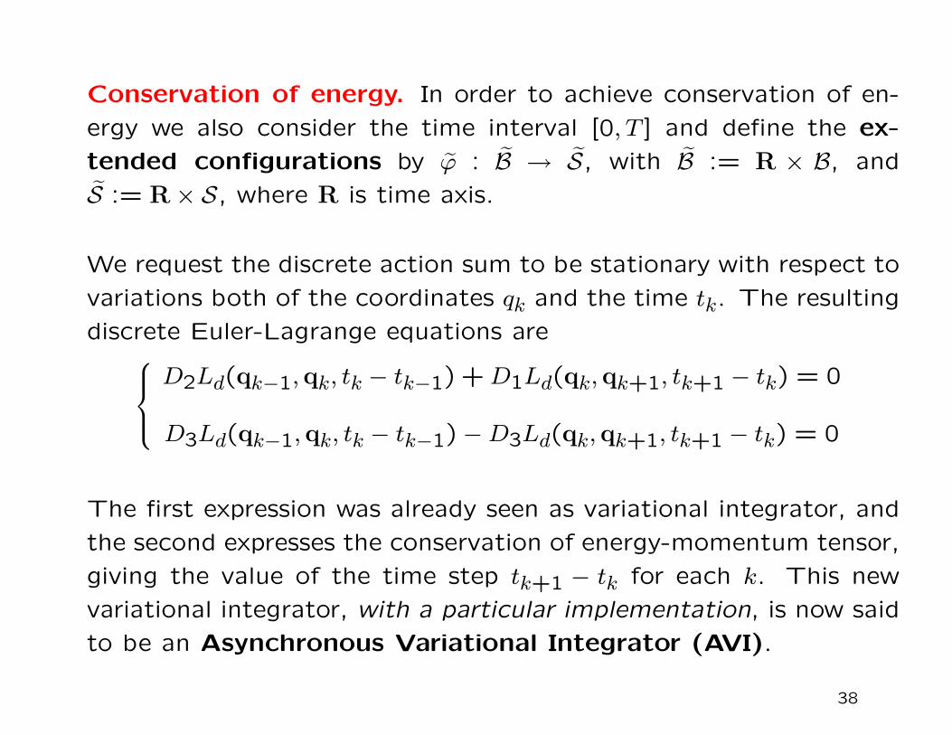
Conservation of energy. In order to achieve conservation of en-

ergy we also consider the time interval [0, T ] and define the ex-

tended configurations by ϕ : B → S, with B := R × B, and

S := R× S, where R is time axis.

We request the discrete action sum to be stationary with respect to

variations both of the coordinates qk and the time tk. The resulting

discrete Euler-Lagrange equations areD2Ld(qk−1,qk, tk − tk−1) +D1Ld(qk,qk+1, tk+1 − tk) = 0

D3Ld(qk−1,qk, tk − tk−1)−D3Ld(qk,qk+1, tk+1 − tk) = 0

The first expression was already seen as variational integrator, and

the second expresses the conservation of energy-momentum tensor,

giving the value of the time step tk+1 − tk for each k. This new

variational integrator, with a particular implementation, is now said

to be an Asynchronous Variational Integrator (AVI).

38

Example : Particles ai in subsystems Kj. The AVI composedby discrete Euler-Lagrange equations is satisfied by solving for boththe coordinates qia and the times tjK

DiaSd = 0

DjKSd = 0

where we consider the discrete action sum as a function of the co-ordinates qia of each particle a and the time t

jK of each subsystem

K. In other words, we restrict the time component tia to coincidewith the time t

jK of one of the subsystem K.

qa0

qaN

K10

K20

K30

K1N

K2N

K3N

39

AVI allow different time steps at different points which is importantfor efficiency. However, the implicit algorithm D

jKSd = 0 is not al-

ways very easy to calculate. Fortunately, the total energy oscillatesaround a constant value for very long time without overall growthor decay, if we choose a particular time step for each cell, in relationboth with the geometry of the mesh, and with material properties.

Example : Evolution over time of the total energy of a thin-shellbeing vibrate

0 0.02 0.04 0.06 0.08 0.1 0.12 0.14 0.16 0.18 0.20

0.05

0.1

0.15

0.2

0.25

0.3

0.35

time

tota

l ene

rgy

green = exterior potential energy, blue = elastic potential energy,black = kinetic energy, red = total energy.

40

Example : Given the discrete Lagrangian

Ld(xk,xk+1, h) = h

(1

2

(xk+1 − xk

h

)TM

(xk+1 − xk

h

)− V (xk)

),

where M is a symmetric, positive definite matrix, and xk are

vector positions in Rn.

Let the triangulation T of B be composed of cells K with nodes a

of mass ma,K such that∑a∈Kma,K = MK, where MK is the mass of

K. The vector positions of K and a at times tjK and tia are denoted

by xjK and xia.

We get an explicit one-step integrator giving the discrete speed

via of node a, at time tia = tjK

ma

xi+1a − xia

ti+1a − tia

= ma

(xia − xi−1

a

tia − ti−1a

)− hK

∂VK

∂xjK(xjK).

41

Convergence of the AVI is known for time steps vanishing toward

zero, for fixed spatial discretization.

Define the maximum time step and the maximum final time

∆tmax = maxK (∆tK) , tmax = maxK (NK∆tK)

Lemma. Consider a sequence of solutions obtained by the appli-

cation of asynchronous variational integrators, to a fixed spatial

discretization, with maximum time step ∆tmax → 0 and maximum

final time tmax → T . Then the final discrete configuration converges

to the exact solution at time T .

Remark. Even for corse mesh we get convergence.

42

Discrete simplicity, and discrete Noether’s theorem for AVI.

One of the powerful features of variational multisymplectic dis-

cretization is that there is a unique discrete multisymplectic struc-

ture, as well as a discrete multisymplectic Lagrangian two-

forms ΩLd.

And the discrete integrator FLd associated to AVI is time-symplectic

ΩLd=(FLd

)∗ΩLd

In the same way it is always possible to define a Noether’s the-

orem for multisymplectic discretization. And so on discrete

symmetries of system are conserved.

43

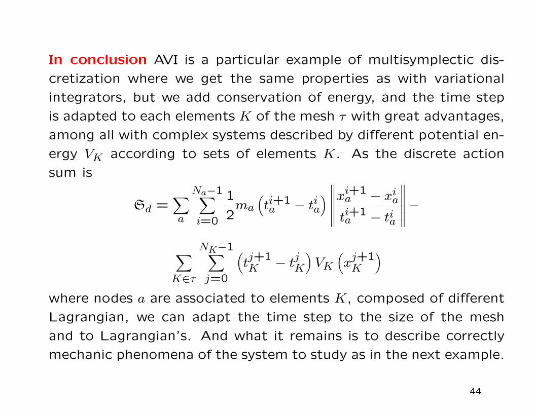
In conclusion AVI is a particular example of multisymplectic dis-

cretization where we get the same properties as with variational

integrators, but we add conservation of energy, and the time step

is adapted to each elements K of the mesh τ with great advantages,

among all with complex systems described by different potential en-

ergy VK according to sets of elements K. As the discrete action

sum is

Sd =∑a

Na−1∑i=0

1

2ma

(ti+1a − tia

) ∥∥∥∥∥∥xi+1a − xiati+1a − tia

∥∥∥∥∥∥−∑K∈τ

NK−1∑j=0

(tj+1K − tjK

)VK

(xj+1K

)where nodes a are associated to elements K, composed of different

Lagrangian, we can adapt the time step to the size of the mesh

and to Lagrangian’s. And what it remains is to describe correctly

mechanic phenomena of the system to study as in the next example.

44

Example : dynamics of thin-shells set, based on Kirchhoff-Love

constraints

0

0.5

1

1.5

2 00.5

1

−0.06

−0.04

−0.02

0

0.02

0.04

0.06

0.08

0.1

0.12

0.14

0

0.5

1

1.5

2 00.5

1

−0.06

−0.04

−0.02

0

0.02

0.04

0.06

0.08

0.1

0.12

0.14

0

0.5

1

1.5

2 00.5

1

−0.06

−0.04

−0.02

0

0.02

0.04

0.06

0.08

0.1

0.12

0.14

0

0.5

1

1.5

2 00.5

1

−0.06

−0.04

−0.02

0

0.02

0.04

0.06

0.08

0.1

0.12

0.14

0

0.5

1

1.5

2 00.5

1

−0.06

−0.04

−0.02

0

0.02

0.04

0.06

0.08

0.1

0.12

0.14

0

0.5

1

1.5

2 00.5

1

−0.06

−0.04

−0.02

0

0.02

0.04

0.06

0.08

0.1

0.12

0.14

45

The advantage of these discrete variational in-

tegrators is that they preserve the symplectic

structure (a classical property of mechanical

systems), and preserve momenta for systems

with symmetry, have excellent energy behavior

(even with some dissipation added), and allow

the usage of different time steps at different

points. These properties significantly enhance

the efficiency of these algorithms.

46