Introduction to Impact evaluation: Methods & Examples

Emmanuel SkoufiasThe World BankPREM KL Forum

May 3-4, 2010

Outline of presentation

1. The Evaluation Problem & Selection Bias

2. Solutions to the evaluation problem Cross- Sectional Estimator

Before and After Estimator

Double Difference Estimator

3. Experimental Designs

4. Quasi-Experimental Designs: PSM, RDD.

5. Instrumental Variables and IE

6. How to implement an Impact evaluation

2

1. Evaluation Problem and Selection Bias

3

How to assess impact

What is beneficiary’s test score with program compared to without program?

Formally, program impact is:

E (Y | T=1) - E(Y | T=0)

Compare same individual with & without programs at same point in time

So what’s the Problem? 4

Solving the evaluation problem

Problem: we never observe the same individual with and without program at same point in time

Observe: E(Y | T=1) & E (Y | T=0) NO!

Solution: estimate what would have happened if beneficiary had not received benefits

Observe: E(Y | T=1) YES!

Estimate: E(Y | T=0) YES!!5

Solving the evaluation problem

Counterfactual: what would have happened without the program

Estimated impact is difference between treated observation and counterfactual

Never observe same individual with and without program at same point in time

Need to estimate counterfactual

Counterfactual is key to impact evaluation6

Finding a good counterfactual

Treated & counterfactual

have identical characteristics,

except for benefiting from the intervention

No other reason for differences in outcomes of treated and counterfactual

Only reason for the difference in outcomes is due to the intervention

7

Having the “ideal” counterfactual……

Y1 (observedl)

Y1* (counterfactual)

Y0

t=0 t=1 time

Intervention

8

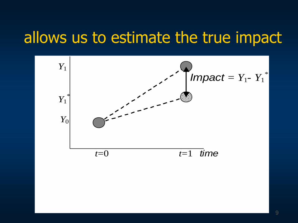
allows us to estimate the true impact

Y1

Impact = Y1- Y1*

Y1*

Y0

t=0 t=1 time

9

Comparison Group Issues

Two central problems:Programs are targeted

Program areas will differ in observable and unobservable ways precisely because the program intended this

Individual participation is (usually) voluntaryParticipants will differ from non-participants in observable

and unobservable ways (selection based on observable variables such as age and education and unobservable variables such as ability, motivation, drive)

Hence, a comparison of participants and an arbitrary group of non-participants can lead to heavily biased results

10

Outcomes (Y) with and without treatment (D) given exogenous covariates (X):

Ti

Ti

Ti XY (i=1,..,n)

Ci

Ci

Ci XY (i=1,..,n)

0)()( 10 iiii XEXE

Gain from the program: Ci

Tii YYG

ATE: average treatment effect: )( iGE

conditional ATE: )()( CTiii XXGE

ATET: ATE on the treated: )1( ii DGE

conditional ATET:

)1,()()1,( iiCi

Ti

CTiiii DXEXDXGE

Archetypal formulation

11

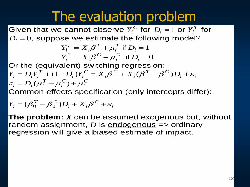
Given that we cannot observe CiY for 1iD or T

iY for

0iD , suppose we estimate the following model? Ti

Ti

Ti XY if 1iD

Ci

Ci

Ci XY if 0iD

Or the (equivalent) switching regression:

iiCT

iC

iC

iiT

iii DXXYDYDY )()1( Ci

Ci

Tiii D )(

Common effects specification (only intercepts differ):

iC

iiCT

i XDY )( 00

The problem: X can be assumed exogenous but, without random assignment, D is endogenous => ordinary regression will give a biased estimate of impact.

The evaluation problem

12

Alternative solutions 1

Experimental evaluation (“Social experiment”) Program is randomly assigned, so that everyone

has the same probability of receiving the treatment.

In theory, this method is assumption free, but in practice many assumptions are required.

Pure randomization is rare for anti-poverty programs in practice, since randomization precludes purposive targeting.

Although it is sometimes feasible to partially randomize.

13

Alternative solutions 2

Non-experimental evaluation (“Quasi-experimental”; “observational studies”)

One of two (non-nested) conditional independence assumptions:

1. Placement is independent of outcome given Xsingle difference methods assuming conditionally

exogenous placement

OR placement is independent of outcomes changesDouble difference methods

2. A correlate of placement is independent of outcomes given D and XInstrumental variables estimator

14

Generic issues

Selection bias

Spillover effects

15

Selection bias in the outcome difference between participants and

non-participants

Observed difference in mean outcomes between participants (D=1) and non-participants (D=0):

)0()1( DYEDYE CT

)1()1( DYEDYE CT

ATET=average treatment effect on the treated

)0()1( DYEDYE CC

Selection bias=difference in mean outcomes (in the absence of the intervention) between participants and non-participants

= 0 with exogenous

program placement

16

Two sources of selection bias

• Selection on observables

Data

Linearity in controls?

• Selection on unobservables

Participants have latent attributes that yield

higher/lower outcomes

• One cannot judge if exogeneity is plausible

without knowing whether one has dealt

adequately with observable heterogeneity.

• That depends on program, setting and data.

17

Spillover effects

• Hidden impacts for non-participants?

• Spillover effects can stem from:

• Markets

• Non-market behavior of participants/non-

participants

• Behavior of intervening agents

(governmental/NGO)

• Example 1: Poor-area programs

• Aid targeted to poor villages+local govt. response

• Example 2: Employment Guarantee Scheme

• assigned program, but no valid comparison group.18

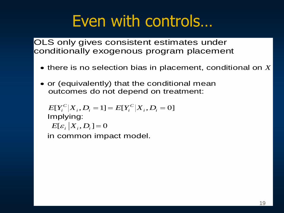
OLS only gives consistent estimates under conditionally exogenous program placement

there is no selection bias in placement, conditional on X

or (equivalently) that the conditional mean outcomes do not depend on treatment:

]0,[]1,[ ii

C

iii

C

i DXYEDXYE

Implying:

0],[ iii DXE

in common impact model.

Even with controls…

19

OLS regression

Ordinary least squares (OLS) estimator of impact

with controls for selection on observables.

controlsRegression controls and matching

Switching regression:

iiCT

iC

iC

iiT

iii DXXYDYDY )()1( Ci

Ci

Tiii D )(

Common effects specification:

iC

iiCT

i XDY )( 00

20

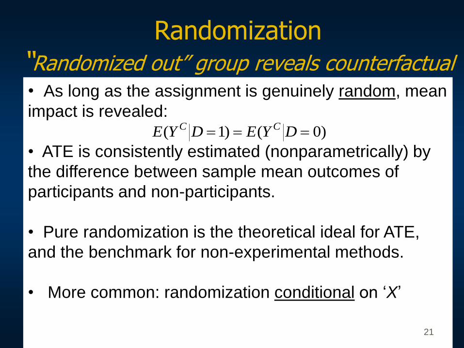
• As long as the assignment is genuinely random, mean

impact is revealed:

• ATE is consistently estimated (nonparametrically) by

the difference between sample mean outcomes of

participants and non-participants.

• Pure randomization is the theoretical ideal for ATE,

and the benchmark for non-experimental methods.

• More common: randomization conditional on „X‟

Randomization“Randomized out” group reveals counterfactual

)0()1( DYEDYE CC

21

2. Impact Evaluation methods

Differ in how they construct the counterfactual• Cross sectional Differences

• Before and After (Reflexive comparisons)

• Difference in Difference (Dif in Dif)

• Experimental methods/Randomization

• Quasi-experimental methods• Propensity score matching (PSM) (not discussed)

• Regression discontinuity design (RDD)

• Econometric methods • Instrumental variables/Encouragement designs

22

Cross-Sectional Estimator

Counterfactual for participants: Non-participant n the same village or hh in similar villages

But then:

Measured Impact = E(Y | T=1) - E(Y | T=0)= True Impact + MSB

where MSB=Mean Selection Bias = MA(T=1) - MA(T=0)

If MA(T=1) > MA(T=0) then MSB>0 and measured impact > true impact

Note: An Experimental or Randomized Design Assigns individuals into T=1 and T=0 groups randomly.

Consequence: MA(T=1) = MA(T=0) MSB=0 and

Measure Impact = True Impact

23

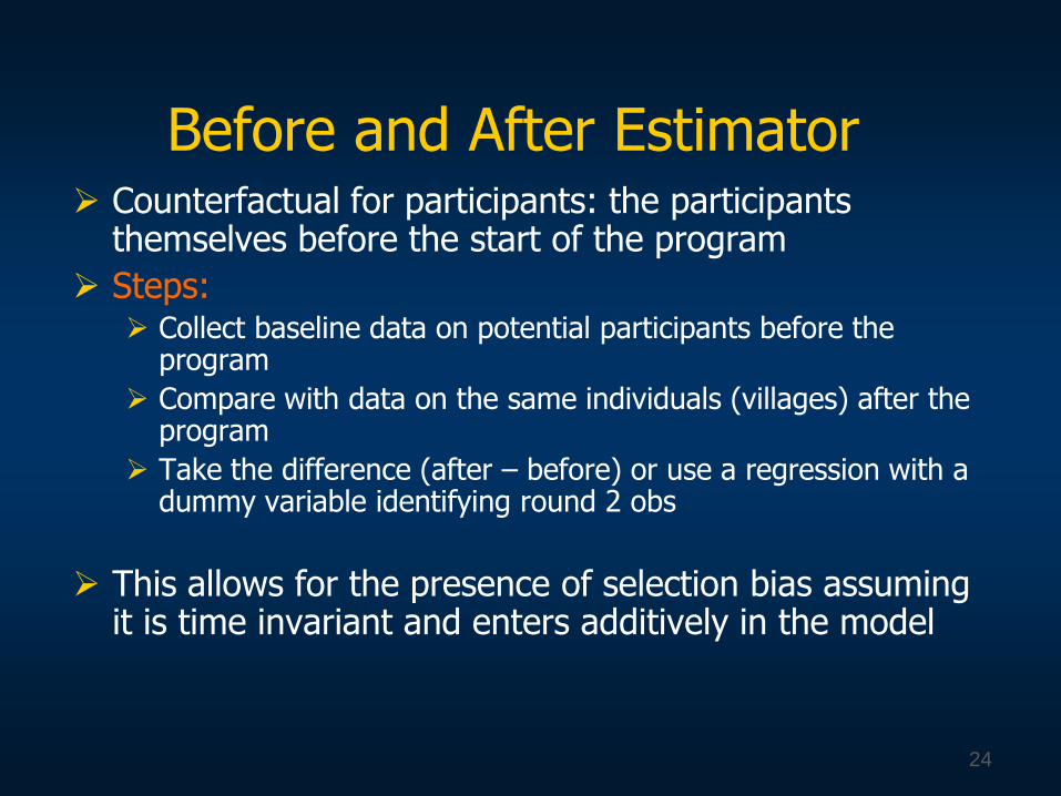
Before and After Estimator Counterfactual for participants: the participants

themselves before the start of the program

Steps: Collect baseline data on potential participants before the

program

Compare with data on the same individuals (villages) after the program

Take the difference (after – before) or use a regression with a dummy variable identifying round 2 obs

This allows for the presence of selection bias assuming it is time invariant and enters additively in the model

24

Before and After Estimator

Y1 (observedl)

Y0

t=0 t=1 time

Intervention

25

Shortcomings of Before and After (BA) comparisons

Not different from “Results Based” Monitoring

Overestimates impactsMeasured Impact = True Impact + Trend

Attribute all changes over time to the program (i.e. assume that there would have been no trend,or no changes in outcomes in the absence of the program)

Note: Difference in difference may be thought as a method that tries to improve upon the BA method

26

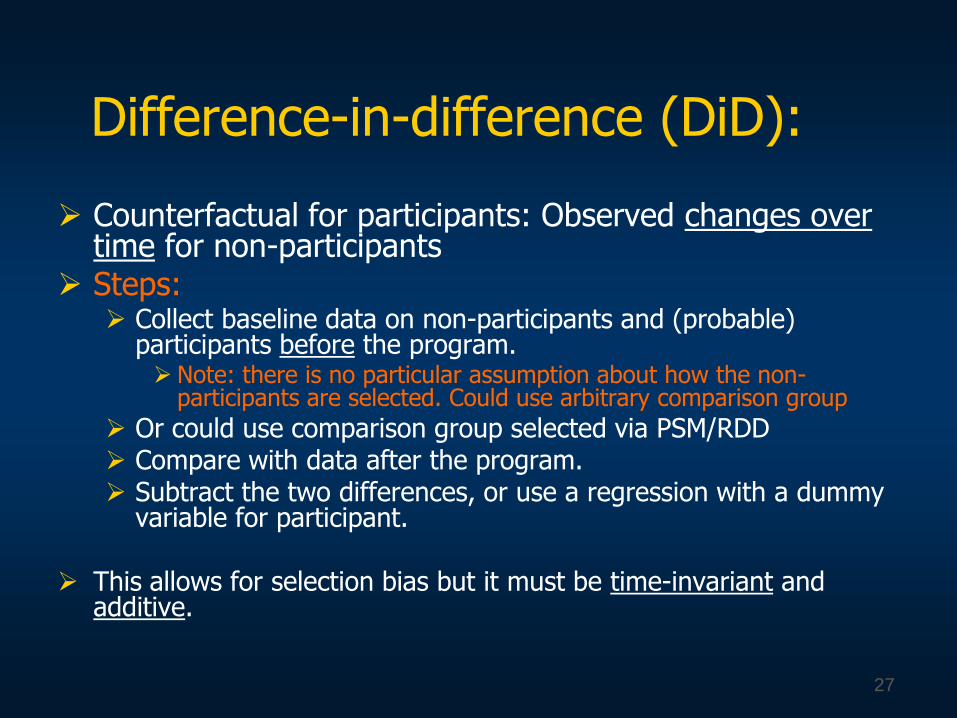
Difference-in-difference (DiD):

Counterfactual for participants: Observed changes over time for non-participants

Steps: Collect baseline data on non-participants and (probable)

participants before the program. Note: there is no particular assumption about how the non-

participants are selected. Could use arbitrary comparison group

Or could use comparison group selected via PSM/RDD Compare with data after the program. Subtract the two differences, or use a regression with a dummy

variable for participant.

This allows for selection bias but it must be time-invariant and additive.

27

Difference-in-difference (DiD): Interpretation 1

Dif-in-Dif removes the trend effect from the estimate of impact using the BA method True impact= Measured Impact in Treat G ( or BA)– Trend

The change in the control group provides an estimate of the trend. Subtracting the “trend” form the change in the treatment group yields the true impact of the program The above assumes that the trend in the C group is an accurate

representation of the trend that would have prevailed in the T group in the absence of the program. That is an assumption that cannot be tested (or very hard to test).

What if the trend in the C group is not an accurate representation of the trend that would have prevailed in the T group in the absence of the program?? Need observations on Y one period before the baseline period.

01 t

CT

t

CT YYYY

C

t

C

t

T

t

T

t YYYY 0101 M easured Im pact – T rend

28

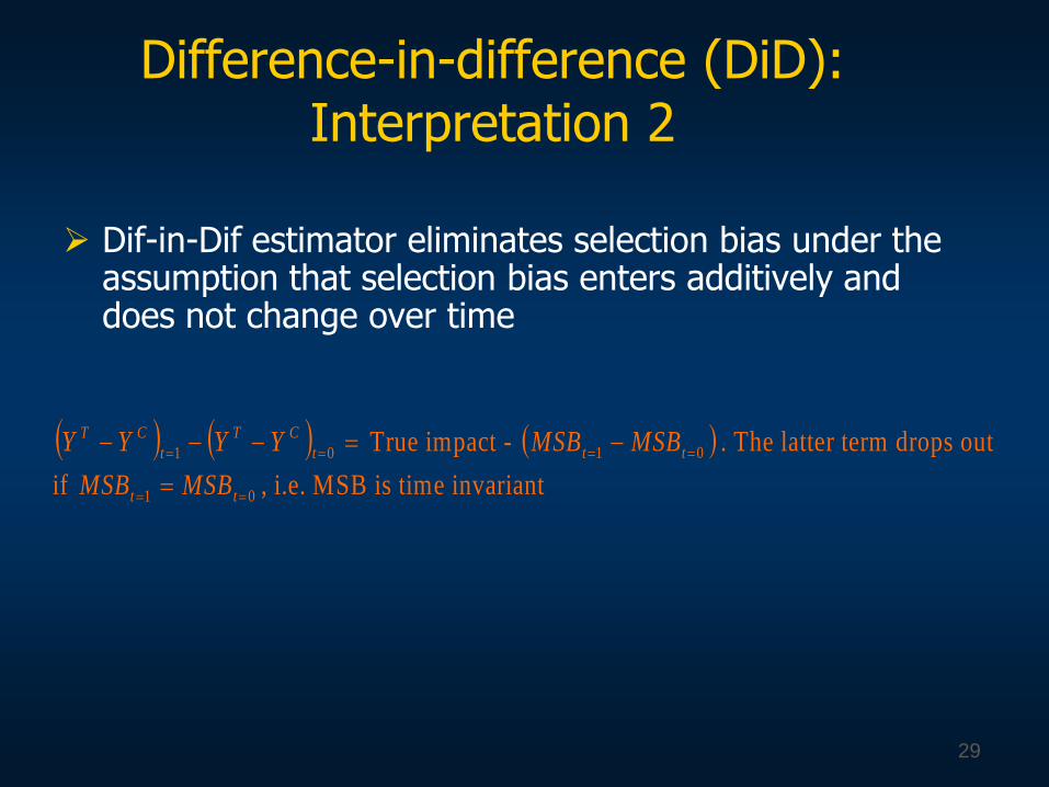
Difference-in-difference (DiD): Interpretation 2

Dif-in-Dif estimator eliminates selection bias under the assumption that selection bias enters additively and does not change over time

01 t

CT

t

CT YYYY True impact - 01 tt MSBMSB . The latter term drops out

if 01 tt MSBMSB , i.e. MSB is time invariant

29

Selection bias

Y1

Impact

Y1*

Y0

t=0 t=1 time

Selection bias

30

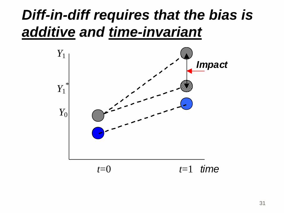
Diff-in-diff requires that the bias is

additive and time-invariant

Y1

Impact

Y1*

Y0

t=0 t=1 time

31

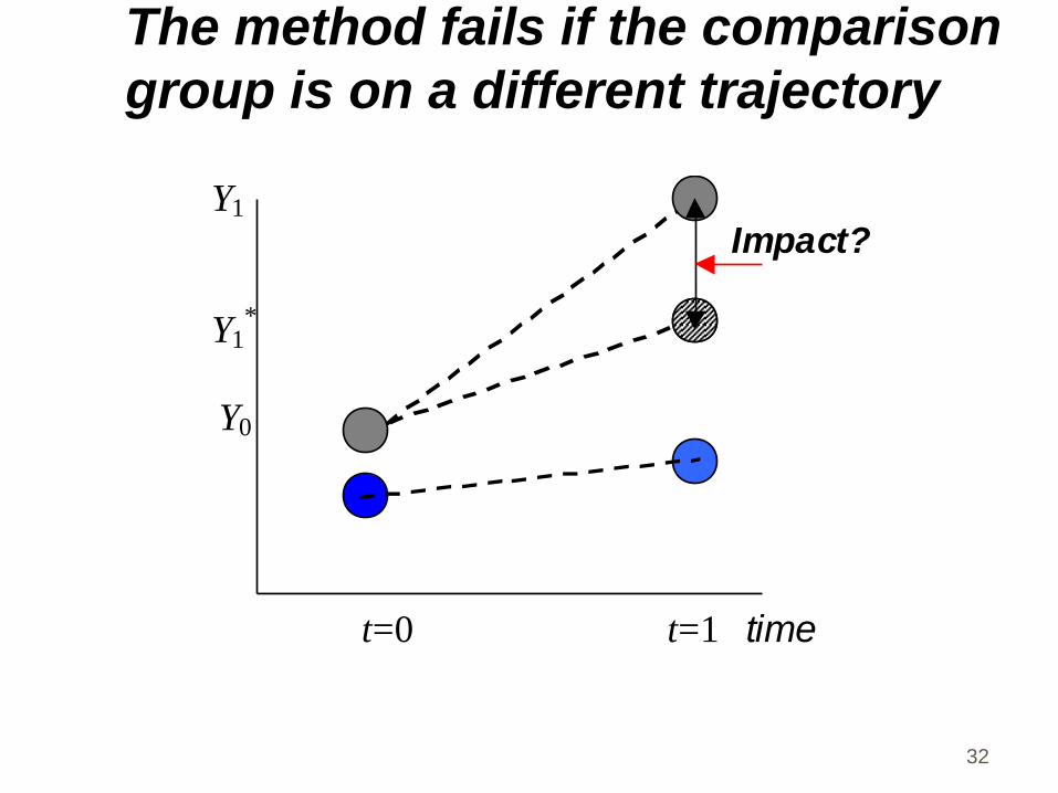
The method fails if the comparison

group is on a different trajectory

Y1

Impact?

Y1*

Y0

t=0 t=1 time

32

3. Experimental Designs

33

The experimental/randomized design

• In a randomized design the control group (randomly assigned out of the program) provides the counterfactual (what would have happened to the treatment group without the program)

• Can apply CSDIFF estimator (ex-post observations only)• Or DiD (if have data in baseline and after start of program)• Randomization equalizes the mean selection bias between T and C

groups

• Note: An Experimental or Randomized Design Assigns individuals into T=1 and T=0 groups randomly. Consequence: MA(T=1) = MA(T=0) MSB=0 and

Measured Impact = True Impact

34

Lessons from practice--1

Ethical objections and political sensitivities

• Deliberately denying a program to those who need it and providing the program to some who do not.

• Yes, too few resources to go around. But is randomization the fairest solution to limited resources?

• What does one condition on in conditional randomizations?

• Intention-to-treat helps alleviate these concerns• => randomize assignment, but free to not

participate• But even then, the “randomized out” group may

include people in great need.=> Implications for design• Choice of conditioning variables.• Sub-optimal timing of randomization• Selective attrition + higher costs 35

Lessons from practice--2

Internal validity: Selective compliance

• Some of those assigned the program choose not to participate.

• Impacts may only appear if one corrects for selective take-up.

• Randomized assignment as IV for participation• Proempleo example: impacts of training only

appear if one corrects for selective take-up

36

Lessons from practice--3

External validity: inference for scaling up

• Systematic differences between characteristics of people normally attracted to a program and those randomly assigned (“randomization bias”: Heckman-Smith)

• One ends up evaluating a different program to the one actually implemented

=> Difficult in extrapolating results from a pilot experiment to the whole population

37

PROGRESA/Oportunidades

What is PROGRESA?

Targeted cash transfer program conditioned on families visiting health centers regularly and on children attending school regularly.

Cash transfer-alleviates short-term poverty

Human capital investment-alleviates poverty in the long-term

By the end of 2004: program (renamed Oportunidades) covered nearly 5 million families, in 72,000 localities in all 31 states (budget of about US$2.5 billion).

38

CCT programs (like PROGRESA)

Expanding

Brazil: Bolsa Familia Colombia: Familias en Acción Honduras: Programa de Asignación Familiar (PRAF) Jamaica: Program of Advancement through Health and Education

(PATH) Nicaragua: Red de Protección Social (RPS) Turkey Ecuador: Bono Solidario Philippines, Indonesia, Peru, Bangladesh: Food for Education

39

Program Description & Benefits Education component

A system of educational grants (details below)

Monetary support or the acquisition of schoolmaterials/supplies

(The above benefits are tied to enrollment and regular (85%) school attendance)

Improved schools and quality of educations (teacher salaries)

40

EXPERIMENTAL DESIGN: Program randomized at the locality level (Pipeline experimental design)

IFPRI not present at time of selection of T and C localities

Report examined differences between T and C for more than 650 variables at the locality level (comparison of locality means) and at the household level (comparison of household means)

Sample of 506 localities– 186 control (no program)– 320 treatment (receive program)

24, 077 Households (hh)78% beneficiariesDifferences between eligible hh and actual beneficiaries receiving benefitsDensification (initially 52% of hh classified as eligible)

PROGRESA/OPORTUNIDADES:

Evaluation Design

41

PROGRESA Evaluation Surveys/Data

BEFORE initiation of program:

–Oct/Nov 97: Household census to select beneficiaries

–March 98: consumption, school attendance, health

AFTER initiation of program

–Nov 98

–June 99

– Nov/Dec 99

Included survey of beneficiary households regarding operations

42

Household Eligibility Status

Discriminant Score

(‘puntaje’)

Localities: 320 Households:14,856

TREATMENT LOCALITY where PROGRESA is in

operation (T=1)

Localities: 186 Households: 9,221

CONTROL

LOCALITY where PROGRESA

operations are delayed (T=0)

Eligible for PROGRESA

benefits (B=1)

Low

Below Threshold

A

B=1, T=1

B

B=1, T=0

Non-Eligible for PROGRESA

benefits (B=0)

Above Threshold

High

C

B=0, T=1

D

B=0, T=0

Table: A Decomposition of the Sample of All Households in Treatment and Control Villages

43

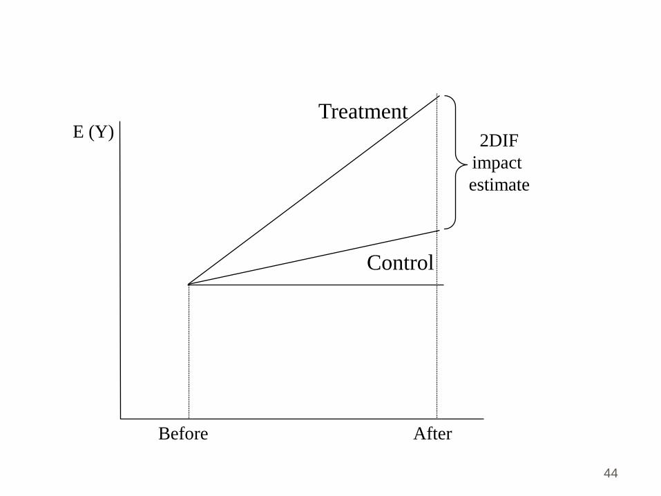
Treatment

Control

E (Y)2DIF

impact

estimate

Before After

44

tviXRiTRiTtiYj jjTRRT ,,)2*(2,

Using regressions to get 2DIF estimates:

•Y(i,t) denotes the value of the outcome indicator in household (or individual) i in period t, •alpha, beta and theta are fixed parameters to be estimated, •T(i) is an binary variable taking the value of 1 if the household belongs in a treatment community and 0 otherwise (i.e., for control communities), •R2 is a binary variable equal to 1 for the second round of the panel (or the round after the initiation of the program) and equal to 0 for the first round (the round before the initiation of the program), •X is a vector of household (and possibly village) characteristics;•last term is an error term summarizing the influence random disturbances.

Limit sample to eligible households in treatment and control and run regression:

a

45

BADIF TRRRTYERTYE XX ,02,1|,12,1|

DIF2 = TR =

CSDIF TRTRTYERTYE XX ,12,0|,12,1|

XX ,02,1|,12,1| RTYERTYE

XX ,02,0|,12,0| RTYERTYE

46

Evaluation Tools

Formal surveys

(Semi)-structured observations and interviews

Focus groups with stakeholders (beneficiaries, local leaders, local PROGRESA officials, doctors, nurses, school teachers, promotoras)

47

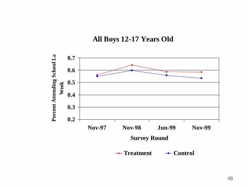
All Boys 12-17 Years Old

0.2

0.3

0.4

0.5

0.6

0.7

Nov-97 Nov-98 Jun-99 Nov-99

Survey Round

Per

cen

t A

tten

din

g S

cho

ol

La

st

Wee

k

Treatment Control

48

All Girls 12-17 Years Old

0.2

0.3

0.4

0.5

0.6

0.7

Nov-97 Nov-98 Jun-99 Nov-99

Survey Round

Percen

t A

tten

din

g S

ch

ool

Last

Week

Treatment Control

49

All Boys 12-17 Years Old

0.20

0.25

0.30

0.35

0.40

Nov-97 Nov-98 Jun-99 Nov-99

Survey Round

Percen

t w

ork

ing L

ast

Week

Treatment Control

50

All Girls 12-17 Years Old

0.05

0.10

0.15

0.20

Nov-97 Nov-98 Jun-99 Nov-99

Survey Round

Per

cen

t W

ork

ing

La

st W

eek

Treatment Control

51

4a. Quasi-Experimental Designs:Propensity Score Matching-PSM

52

53

Introduction By consensus, a randomized design

provides the most credible method of evaluating program impact.

But experimental designs are difficult to implement and are accompanied by political risks that jeopardize the chances of implementing them The idea of having a comparison/control group

is very unappealing to program managers and governments

ethical issues involved in withholding benefits for a certain group of households

Propensity-score matching (PSM)

Builds on this fundamental idea of the randomized design and uses it to come up a control group (under some maintained/untested assumptions).

In an experimental design a treatment and a control have equal probability in joining the program. Two people apply and we decide who gets the program by a coin toss, then each person has probability of 50% of joining the program

54

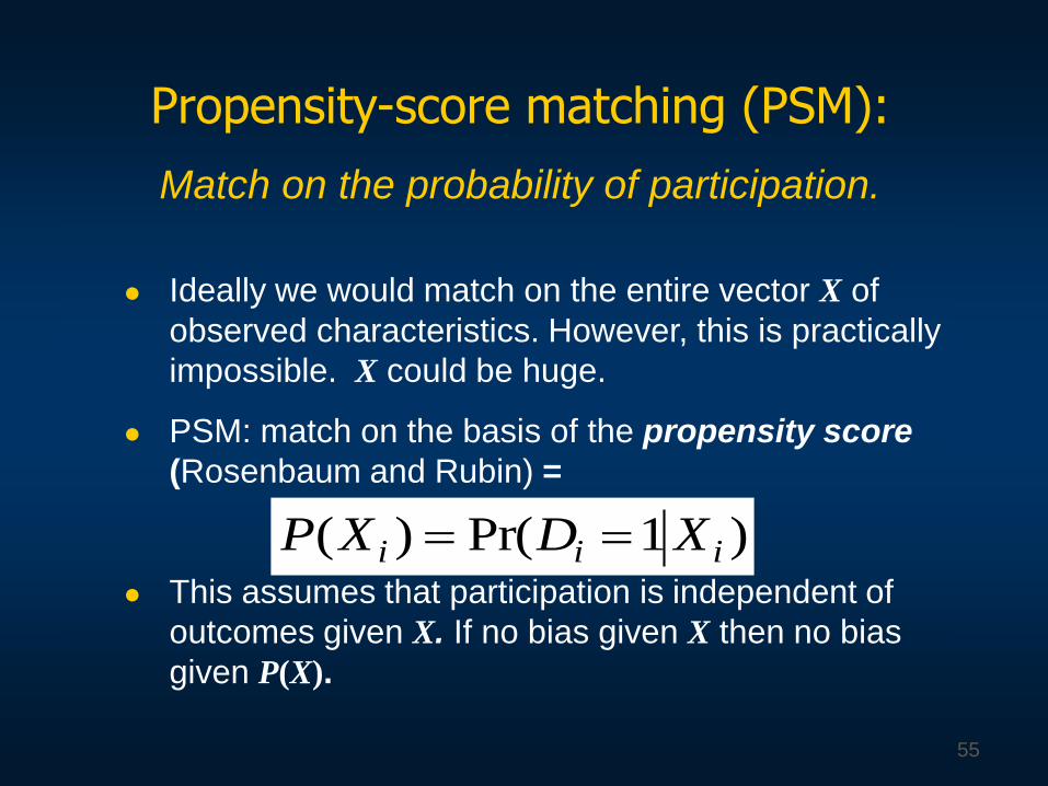
Ideally we would match on the entire vector X of

observed characteristics. However, this is practically

impossible. X could be huge.

PSM: match on the basis of the propensity score

(Rosenbaum and Rubin) =

This assumes that participation is independent of

outcomes given X. If no bias given X then no bias

given P(X).

Propensity-score matching (PSM):

Match on the probability of participation.

)1Pr()( iii XDXP

55

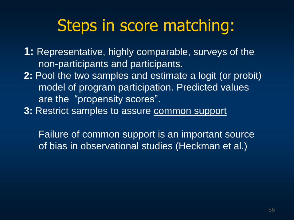
1: Representative, highly comparable, surveys of the

non-participants and participants.

2: Pool the two samples and estimate a logit (or probit)

model of program participation. Predicted values

are the “propensity scores”.

3: Restrict samples to assure common support

Failure of common support is an important source

of bias in observational studies (Heckman et al.)

Steps in score matching:

56

Propensity-score matching (PSM)

You choose a control group by running a logit/probit where on the LHS you have a binary variable =1 if a person is in the program, 0 otherwise, as a function of observed characteristics.

Based on this logit/probit, one can derive the predicted probability of participating into the program (based on the X or observed characteristics) and you choose a control group for each treatment individual/hh using hh that are NOT in the program and have a predicted probability of being in the program very close to that of the person who is in the program (nearest neighbor matching, kernel matching etc).

Key assumption: selection in to the program is based on observables (or in other words unobservables are not important in determining participation into the program).

57

Density

0 1 Propensity score

Density of scores for participants

58

Density

0 1 Propensity score

Density of scores for non-participants

59

Density

0 Region of common support 1 Propensity score

Density of scores for non-participants

60

5: For each participant find a sample of non-

participants that have similar propensity

scores.

6: Compare the outcome indicators. The

difference is the estimate of the gain due

to the program for that observation.

7: Calculate the mean of these individual

gains to obtain the average overall gain.

Various weighting schemes =>

Steps in PSM cont.,

61

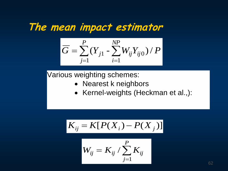
The mean impact estimator

NP

iijij

P

jj PYW - Y G

10

11 /)(

Various weighting schemes:

Nearest k neighbors

Kernel-weights (Heckman et al.,):

KK WP

jijijij

1

/

)]()([ jiij XPXPKK

62

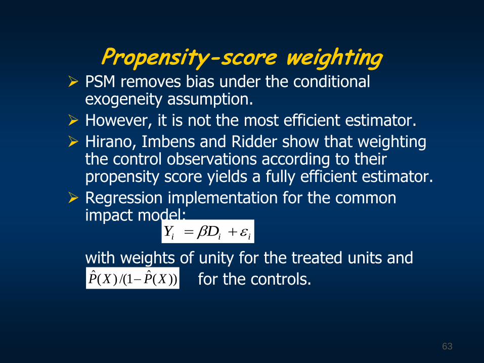
Propensity-score weighting PSM removes bias under the conditional

exogeneity assumption.

However, it is not the most efficient estimator.

Hirano, Imbens and Ridder show that weighting the control observations according to their propensity score yields a fully efficient estimator.

Regression implementation for the common impact model:

with weights of unity for the treated units and

for the controls.

iii DY

))(ˆ1/()(ˆ XPXP

63

How does PSM compare to an experiment?

PSM is the observational analogue of an experiment in which placement is independent of outcomes

The difference is that a pure experiment does not require the untestable assumption of independence conditional on observables.

Thus PSM requires good data.

Example of Argentina’s Trabajar program

Plausible estimates using SD matching on good data

Implausible estimates using weaker data64

How does PSM differ from OLS?

PSM is a non-parametric method (fully non-parametric in outcome space; optionally non-parametric in assignment space)

Restricting the analysis to common support

=> PSM weights the data very differently to standard OLS regression

In practice, the results can look very different!

65

How does PSM perform relative to other methods?

In comparisons with results of a randomized experiment on a US training program, PSM gave a good approximation (Heckman et al.; Dehejia and Wahba)

Better than the non-experimental regression-based methods studied by Lalonde for the same program.

However, robustness has been questioned (Smith and Todd)

66

Lessons on matching methods

When neither randomization nor a baseline survey are feasible, careful matching is crucial to control for observable heterogeneity.

Validity of matching methods depends heavily on data quality. Highly comparable surveys; similar economic environment

Common support can be a problem (esp., if treatment units are lost).

Look for heterogeneity in impact; average impact may hide important differences in the characteristics of those who gain or lose from the intervention.

67

4b. Quasi-Experimental Designs:Regression Discontinuity Design-RDD

68

Pipeline comparisons• Applicants who have not yet received program

form the comparison group

• Assumes exogeneous assignment amongst

applicants

• Reflects latent selection into the program

Exploiting program design

69

Lessons from practice

Know your program well: Program design features can be very useful for identifying impact.

Know your setting well too: Is it plausible that outcomes are continuous under the counterfactual?

But what if you end up changing the program to identify impact? You have evaluated something else!

70

Introduction

Alternative: Quasi-experimental methods attempting to equalize selection bias between treatment and control groups

Discuss paper using PROGRESA data (again)one of the first to evaluate the performance of

RDD in a setting where it can be compared to experimental estimates.

Focus on school attendance and work of 12-16 yr old boys and girls.

71

Discontinuity designs• Participate if score M < m

• Impact=

• Key identifying assumption: no discontinuity in

counterfactual outcomes at m

Regression Discontinuity Design: RDD

)()( mMYEmMYE iC

iiT

i

72

Indexes are common in targeting of social programs

Anti-poverty programs targeted to

households below a given poverty index

Pension programs targeted to

population above a certain age

Scholarships targeted to students with

high scores on standardized test

CDD Programs awarded to NGOs that

achieve highest scores

Others:

Credit scores in Bank lending

73

Advantages of RDD for Evaluation

RDD yields an unbiased estimate of treatment effect at the discontinuity

Can many times take advantage of a known rule for assigning the benefit that are common in the designs of social policy

No need to “exclude” a group of eligible households/individuals from treatment

74

Potential Disadvantages of RD

Local treatment effects cannot be generalized (especially if there

is heterogeneity of impacts)

Power: effect is estimated at the discontinuity, so we

generally have fewer observations than in a randomized experiment with the same sample size

Specification can be sensitive to functional form: make sure the relationship between the assignment variable and the outcome variable is correctly modeled, including: Nonlinear Relationships Interactions

75

Some Background on PROGRESA’s targeting

Two-stage Selection process:Geographic targeting (used census data to

identify poor localities)Within Village household-level targeting

(village household census)Used hh income, assets, and demographic

composition to estimate the probability of being poor (Inc per cap<Standard Food basket).

Discriminant analysis applied separately by regionDiscriminant score of each household compared to a

threshold value (high DS=Noneligible, low DS=Eligible)

Initially 52% eligible, then revised selection process so that 78% eligible. But many of the “new poor” households did not receive benefits

76

Figure 1: Kernel Densities of Discriminant Scores and Threshold points by region

Density

Region 3Discriminant Score

759

3.9e-06

.003412

Density

Region 4Discriminant Score

753

2.8e-06

.00329

Density

Region 5Discriminant Score

751

0

.002918

Density

Region 6Discriminant Score

752

5.5e-06

.004142

Density

Region 12Discriminant Score

571

8.0e-06

.004625

Density

Region 27Discriminant Score

691

4.5e-06

.003639

Density

Region 28Discriminant Score

757

.000015

.002937

77

The RDD method-1

A quasi-experimental approach based on the discontinuity of the treatment assignment mechanism.

Sharp RD design Individuals/households are assigned to treatment (T) and

control (NT) groups based solely on the basis of an observed continuous measure such as the discriminate score DS. For example, B =1 if and only if DS<=COS (B=1 eligible beneficiary) and B=0 otherwise . Propensity is a step function that is discontinuous at the point DS=COS.

Analogous to selection on observables only.

Violates the strong ignorability assumption of Rosenbaum and Rubin (1983) which also requires the overlap condition.

78

The RDD method-2

Fuzzy RD designTreatment assignment depends on an observed

continuous variable such as the discriminant score DS but in a stochastic manner. Propensity score is S-shaped and is discontinuous at the point DS=COS.

Analogous to selection on observables and unobservables.

Allows for imperfect compliance (self-selection, attrition) among eligible beneficiaries and contamination of the comparison group by non-compliance (substitution bias).

79

______ Sharp Design

--------- Fuzzy design

Regression Discontinuity Design; treatment assignment in sharp (solid) and fuzzy (dashed) designs.

80

Kernel Regression Estimator of Treatment Effect with a Sharp RDD

COSDSYECOSDSYEYYCOS ii

COSDSii

COSDS

|lim|lim

n

i ii

n

i iii

uK

uKYY

1

1

)(*

)(**

where

and

n

i ii

n

i iii

uK

uKYY

1

1

)(*)1(

)(*)1(*

Alternative estimators (differ in the way local information is exploited and in the set of regularity conditions required to achieve asymptotic properties):

Local Linear Regression (HTV, 2001) Partially Linear Model (Porter, 2003) 81

2DIF CSDIF CSDIF-50 Uniform Biweight Epanechnik Triangular Quartic Guassian

SCHOOL (1) (2) (3) (4) (5) (6) (7) (8) (9)

Round 1 n.a 0.013 -0.001 -0.053 -0.016 -0.031 -0.018 -0.016 -0.050

st. error 0.018 0.028 0.027 0.031 0.029 0.031 0.031 0.021

Round 3 0.050 0.064 0.071 0.020 0.008 0.010 0.008 0.008 0.005

st. error 0.017 0.019 0.028 0.028 0.034 0.031 0.033 0.034 0.022

Round 5 0.048 0.061 0.099 0.052 0.072 0.066 0.069 0.072 0.057

st. error 0.020 0.019 0.030 0.028 0.032 0.030 0.032 0.032 0.021

Nobs 4279

R-Squared 0.25

WORK

Round 1 n.a. 0.018 0.007 0.012 -0.016 -0.004 -0.013 -0.016 0.025

st. error 0.019 0.029 0.027 0.032 0.029 0.031 0.032 0.021

Round 3 -0.037 -0.018 -0.007 0.007 -0.004 0.002 0.001 -0.004 0.005

st. error 0.023 0.017 0.029 0.024 0.028 0.026 0.028 0.028 0.019

Round 5 -0.046 -0.028 -0.037 -0.031 -0.029 -0.030 -0.029 -0.029 -0.028

st. error 0.025 0.017 0.025 0.024 0.028 0.026 0.027 0.028 0.019

Nobs 4279

R-Squared 0.19

NOTES:

Estimates in bold have t-values >=2

Treatment Group for Experimental & RDD Estimates: Beneficiary Households in Treatment Villages (Group A)

Comparison Group for Experimental Estimates: Eligible Households in Control Villages (Group B)

Comparison Group for RDD Estimates: NonEligible Households in Treatment Villages (Group C)

16331

0.21

16331

0.16

TABLE 3a

Estimates of Program Impact By Round (BOYS 12-16 yrs old)

RDD Impact Estimates using different kernel functions

Experimental Estimates

82

2DIF CSDIF CSDIF-50 Uniform Biweight Epanechnik. Triangular Quartic Guassian

SCHOOL (1) (2) (3) (4) (5) (6) (7) (8) (9)

Round 1 n.a. -0.001 0.000 -0.027 -0.025 -0.026 -0.025 -0.025 -0.035

st. error 0.020 0.030 0.029 0.036 0.033 0.034 0.036 0.023

Round 3 0.086 0.085 0.082 0.038 0.039 0.041 0.039 0.039 0.054

st. error 0.017 0.020 0.029 0.030 0.036 0.033 0.034 0.036 0.024

Round 5 0.099 0.098 0.099 0.078 0.114 0.097 0.107 0.114 0.084

st. error 0.020 0.019 0.028 0.031 0.036 0.033 0.035 0.036 0.025

Nobs 3865

R-Squared 0.23

WORK

Round 1 n.a. 0.034 0.000 0.033 0.026 0.027 0.027 0.026 0.030

st. error 0.017 0.024 0.019 0.022 0.020 0.021 0.022 0.015

Round 3 -0.034 0.000 0.001 0.005 0.001 0.003 0.002 0.001 -0.008

st. error 0.017 0.009 0.016 0.015 0.018 0.016 0.017 0.018 0.012

Round 5 -0.042 -0.008 -0.025 -0.019 -0.034 -0.029 -0.033 -0.034 -0.025

st. error 0.019 0.009 0.018 0.015 0.018 0.017 0.018 0.018 0.013

Nobs 3865

R-Squared 0.07

NOTES:

Estimates in bold have t-values >=2

Treatment Group for Experimental & RDD Estimates: Beneficiary Households in Treatment Villages (Group A)

Comparison Group for Experimental Estimates: Eligible Households in Control Villages (Group B)

Comparison Group for RDD Estimates: NonEligible Households in Treatment Villages (Group C)

15046

0.22

15046

0.05

TABLE 3b

Estimates of Program Impact By Round (GIRLS 12-16 yrs old)

RDD Impact Estimates using different kernel functions

Experimental Estimates

83

Main Results

Overall the performance of the RDD is remarkably good.

The RDD estimates of program impact agree with the experimental estimates in 10 out of the 12 possible cases.

The two cases in which the RDD method failed to reveal any significant program impact on the school attendance of boys and girls are in the first year of the program (round 3).

84

5. Instrumental variables/Encouragement Designs

85

5. Instrumental variablesIdentifying exogenous variation using a 3rd variable

Outcome regression:

(D = 0,1 is our program – not random)

• “Instrument” (Z) influences participation, but does not affect outcomes given participation (the “exclusion restriction”).

• This identifies the exogenous variation in outcomes due to the program.

Treatment regression:

iii DY

iii uZD

86

Reduced-form outcome regression:

where and

Instrumental variables (two-stage least squares)

estimator of impact:

Or:

iiiiii ZuZY )(

OLSOLSIVE ˆ/ˆˆ

iii u

iii ZY )ˆ(

Predicted D purged of endogenous part.87

Problems with IVE1. Finding valid IVs;

Usually easy to find a variable that is correlated with treatment.

However, the validity of the exclusion restrictions is often questionable.

2. Impact heterogeneity due to latent factors

88

Sources of instrumental variables

Partially randomized designs as a source of IVs

Non-experimental sources of IVs

Geography of program placement (Attanasio and Vera-Hernandez); “Dams” example (Duflo and Pande)

Political characteristics (Besley and Case; Paxson and Schady)

Discontinuities in survey design

89

Endogenous compliance: Instrumental variables estimator

D =1 if treated, 0 if control

Z =1 if assigned to treatment, 0 if not.

Compliance regression

Outcome regression(“intention to treat effect”)

2SLS estimator (=ITT deflated by compliance rate)

iii ZD 11

iii ZY 22

1

2

ˆ

ˆ

90

Essential heterogeneity and IVECommon-impact specification is not harmless.Heterogeneity in impact can arise from

differences between treated units and the counterfactual in latent factors relevant to outcomes.

For consistent estimation of ATE we must assume that selection into the program is unaffected by latent, idiosyncratic, factors determining the impact (Heckman et al).

However, likely “winners” will no doubt be attracted to a program, or be favored by the implementing agency.

=> IVE is biased even with “ideal” IVs.

91

Stylized example Two types of people (1/2 of each):

Type H: High impact; large gains (G) from program Type L: Low impact: no gain

Evaluator cannot tell which is which But the people themselves can tell (or have a useful

clue)

Randomized pilot: Half goes to each type Impact=G/2

Scaled up program: Type H select into program; Type L do not Impact=G

92

IVE identifies the effect for those induced to switch by

the instrument (“local average effect”)

Suppose Z takes 2 values. Then the effect of the

program is:

Care in extrapolating to the whole population when

there is latent heterogeneity.

IVE is only a ‘local’ effect

)0|()1|(

)0|()1|(

ZDEZDE

ZYEZYEIVE

93

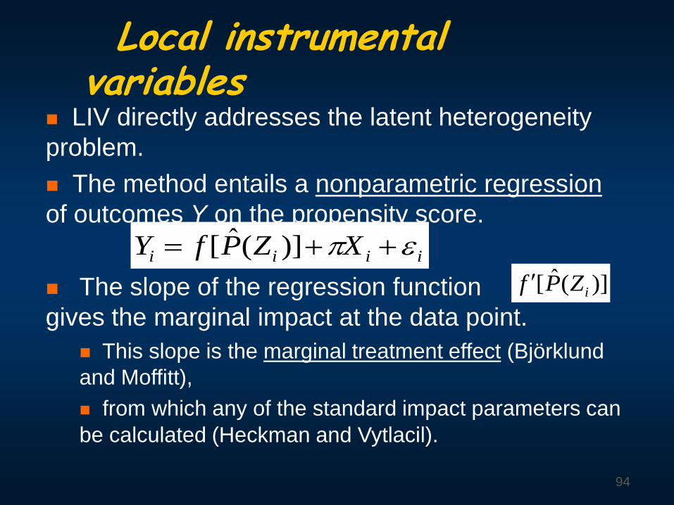
LIV directly addresses the latent heterogeneity

problem.

The method entails a nonparametric regression

of outcomes Y on the propensity score.

The slope of the regression function

gives the marginal impact at the data point.

This slope is the marginal treatment effect (Björklund

and Moffitt),

from which any of the standard impact parameters can

be calculated (Heckman and Vytlacil).

Local instrumental variables

iiii XZPfY )](ˆ[

)](ˆ[ iZPf

94

Lessons from practice

Partially randomized designs offer great source of IVs.

The bar has risen in standards for non-experimental IVE Past exclusion restrictions often questionable in

developing country settings

However, defensible options remain in practice, often motivated by theory and/or other data sources

Future work is likely to emphasize latent heterogeneity of impacts, esp., using LIV.

95

6. How to Implement an Impact Evaluation

96

Timeline

T1 T2 T3 T4 T5 T6 T7 T8

Treatment Start of intervention

Control Start of intervention

SURVEYS Follow-up Follow-up

Program

Implementation

Timeline

Impact EvaluationBaseline

Baseline survey must go into field before program implemented

Exposure period between Treatment and Control areas is subject to political, logistical considerations

Follow up survey must go into field before program implemented in Control areas

Additional follow up surveys depend on funding and marginal benefits

97

Prepare & plan evaluation at same time preparing intervention

Avoid conflicts with operational needs

Strengthen intervention design and results framework

Prospective designs:

Key to finding control groups

More flexibility before publicly presenting roll-out plan

Better able to deal with ethical and stakeholder issues

Lower costs of the evaluation98

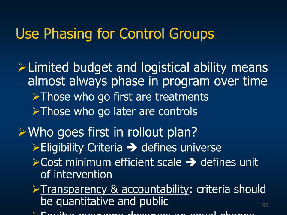
Use Phasing for Control Groups

Limited budget and logistical ability means almost always phase in program over timeThose who go first are treatments

Those who go later are controls

Who goes first in rollout plan?Eligibility Criteria defines universe

Cost minimum efficient scale defines unit of intervention

Transparency & accountability: criteria should be quantitative and public

Equity: everyone deserves an equal chance99

Monitoring Data can be used for Impact Evaluation

Program monitoring data usually only collected in areas where active

Start in control areas at same time as in treatment areas for baseline

Add outcome indicators into monitoring data collection

Very cost-effective as little need for additional special surveys

100

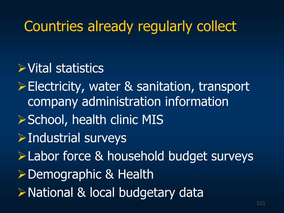
Countries already regularly collect

Vital statistics

Electricity, water & sanitation, transport company administration information

School, health clinic MIS

Industrial surveys

Labor force & household budget surveys

Demographic & Health

National & local budgetary data101

Can these other data be used?

Critical issuesDo they collect outcome indicators

Can we identify controls and treatmentsi.e. link to intervention locations and/or

beneficiaries

question of identification codes

Statistical power: are there sufficient sample sizes in treatment and control areas

Are there baseline (pre-intervention data)

Are there more than one year prior to test for equality of pre-intervention trends

True for census data & vital statistics

Usually not for survey data 102

Special Surveys

Where there is no monitoring system in place or available data is incomplete

Need baseline & follow-up of control & treatments

May need information that do not want to collect on a regular basis (esp specific outcomes)

Options

Collect baseline as part of program application process

If controls never apply, then need special survey 103

Sample Sizes

Should be based on power calculations

Sample sizes needed to statistically distinguished between two means

Increases the rarer the outcome (e.g maternal mortality)

Increases the larger the standard deviation of the outcome indicator (e.g. test scores)

Increases the smaller the desired effect size

Need more sample for subpopulation analysis (gender, poverty)

104

Staffing Options

Contract a single firmEasy one stop shopping & responsibility clear

Less flexible & expensive

Few firms capable, typically large international firms only ones with all skills

Split responsibilityContract one for design, questionnaire content,

supervision of data collection, and analysis

Contract another for data collection

More complex but cheaper

Can get better mix of skills & use local talent 105

Staffing In-country Lead coordinator

Assists in logistical coordination

Based in-country to navigate obstacles

Can be external consultant, or in-country researcher

Must have stake in the successful implementation of field work

Consultants (International?)

Experimental Design and analysis

Questionnaire and sample design

Local research firm

Responsible for field work and data entry

Local researchers (work with international?) 106

Budget: How much will you need?

Single largest component: Data collection

Cost depends on sample size, interview length & measurement

Do you need a household survey?

Do you need a institutional survey?

What are your sample sizes?

What is the geographical distribution of your sample?

107

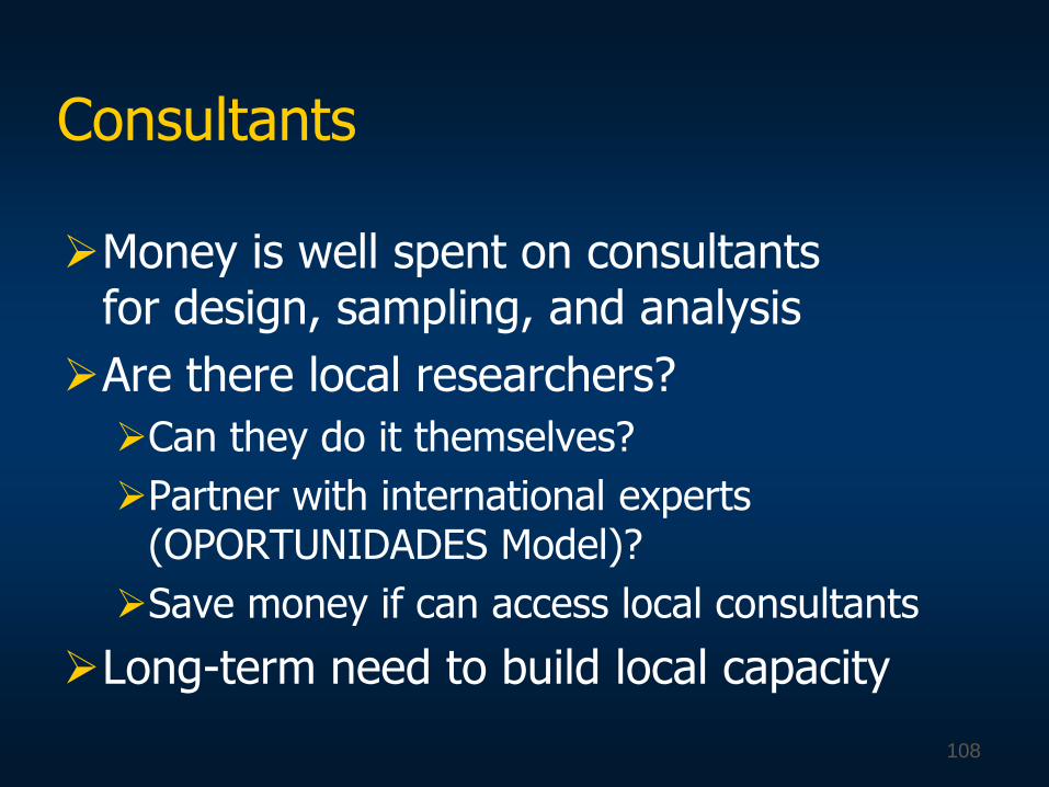
Consultants

Money is well spent on consultants for design, sampling, and analysis

Are there local researchers?

Can they do it themselves?

Partner with international experts (OPORTUNIDADES Model)?

Save money if can access local consultants

Long-term need to build local capacity

108

Monitoring the Intervention

Supervise the program implementation

Evaluation design is based on roll-out plan

Ensure program implementation follows roll-out plan

In order to mitigate problems with program implementation:

Maintain dialogue with government

Build support for impact evaluation among other donors, key players

109

Building Support for Impact Evaluation

Once Evaluation Plan for design and implementation is determined:

Present plan to government counterparts

Present plan to key players (donors, NGOs, etc.)

Present plan to other evaluation experts

110

Operational messages

Plan evaluation at same time plan project

Build an explicit evaluation team

Influence roll-out to obtain control groups

Use quantitative & public allocation criteria

Randomization is ethical

Strengthen monitoring systems to improve IE quality & lower costs

Sample sizes of surveys drive budget 111

Thank you

112