106
Ching-Shan Chou and Avner Friedman Introduction to Mathematical Biology April 8, 2015 Springer

Ching-Shan Chou and Avner Friedman
Introduction to MathematicalBiology
April 8, 2015
Springer

Contents
1 Introduction . . . . . . . . . . . . . . . . . . . . . . . . . . . . . . . . . . . . . . . . . . . . . . . . . . . 1
2 Bacterial Growth in Chemostat . . . . . . . . . . . . . . . . . . . . . . . . . . . . . . . . . . 32.1 Numerical Simulations – Introduction to MATLAB . . . . . . . . . . . . . . 9
2.1.1 Scalar calculations . . . . . . . . . . . . . . . . . . . . . . . . . . . . . . . . . . . 102.1.2 Vector and matrix operations . . . . . . . . . . . . . . . . . . . . . . . . . . . 112.1.3 Numerical algorithms of solving ODE . . . . . . . . . . . . . . . . . . . 15
3 Linear Differential Equations . . . . . . . . . . . . . . . . . . . . . . . . . . . . . . . . . . . 173.1 Numerical Simulations . . . . . . . . . . . . . . . . . . . . . . . . . . . . . . . . . . . . . . 21
3.1.1 Solving a second order ODE . . . . . . . . . . . . . . . . . . . . . . . . . . . 213.1.2 Plotting figures . . . . . . . . . . . . . . . . . . . . . . . . . . . . . . . . . . . . . . 22
4 Systems of two differential equations . . . . . . . . . . . . . . . . . . . . . . . . . . . . . 254.1 Numerical Simulations . . . . . . . . . . . . . . . . . . . . . . . . . . . . . . . . . . . . . . 27
5 Predator-Prey Models . . . . . . . . . . . . . . . . . . . . . . . . . . . . . . . . . . . . . . . . . . 315.1 Numerical Simulations . . . . . . . . . . . . . . . . . . . . . . . . . . . . . . . . . . . . . . 35
6 Two competing populations . . . . . . . . . . . . . . . . . . . . . . . . . . . . . . . . . . . . . 376.1 Numerical Simulations . . . . . . . . . . . . . . . . . . . . . . . . . . . . . . . . . . . . . . 41
6.1.1 Revisiting Euler method for solving ODE – consistencyand convergence . . . . . . . . . . . . . . . . . . . . . . . . . . . . . . . . . . . . . 41
6.1.2 Backward Euler Method . . . . . . . . . . . . . . . . . . . . . . . . . . . . . . 42
7 General systems of differential equations . . . . . . . . . . . . . . . . . . . . . . . . . 457.1 Numerical Simulations . . . . . . . . . . . . . . . . . . . . . . . . . . . . . . . . . . . . . . 48
8 The chemostat model revisited . . . . . . . . . . . . . . . . . . . . . . . . . . . . . . . . . . . 498.1 Numerical Simulations . . . . . . . . . . . . . . . . . . . . . . . . . . . . . . . . . . . . . . 51
8.1.1 Bisection Method . . . . . . . . . . . . . . . . . . . . . . . . . . . . . . . . . . . 528.1.2 Newton’s Method . . . . . . . . . . . . . . . . . . . . . . . . . . . . . . . . . . . 53
3
4 Contents
9 Spread of Disease . . . . . . . . . . . . . . . . . . . . . . . . . . . . . . . . . . . . . . . . . . . . . . 559.1 Numerical Simulations . . . . . . . . . . . . . . . . . . . . . . . . . . . . . . . . . . . . . . 59
10 Enzyme Dynamics . . . . . . . . . . . . . . . . . . . . . . . . . . . . . . . . . . . . . . . . . . . . . . 6310.1 Numerical Simulations . . . . . . . . . . . . . . . . . . . . . . . . . . . . . . . . . . . . . . 69
11 Bifurcation Theory . . . . . . . . . . . . . . . . . . . . . . . . . . . . . . . . . . . . . . . . . . . . . 7111.1 Endangered Species . . . . . . . . . . . . . . . . . . . . . . . . . . . . . . . . . . . . . . . . 7611.2 Numerical Simulations . . . . . . . . . . . . . . . . . . . . . . . . . . . . . . . . . . . . . . 77
12 Atherosclerosis: the risk of high cholesterol . . . . . . . . . . . . . . . . . . . . . . . 8112.1 Numerical Simulations . . . . . . . . . . . . . . . . . . . . . . . . . . . . . . . . . . . . . . 84
13 Cancer-immune Interaction . . . . . . . . . . . . . . . . . . . . . . . . . . . . . . . . . . . . . 8513.1 Numerical Simulations . . . . . . . . . . . . . . . . . . . . . . . . . . . . . . . . . . . . . . 88
14 Cancer Therapy . . . . . . . . . . . . . . . . . . . . . . . . . . . . . . . . . . . . . . . . . . . . . . . 9114.0.1 VEGF receptor inhibitor . . . . . . . . . . . . . . . . . . . . . . . . . . . . . . 9114.0.2 Virotherapy . . . . . . . . . . . . . . . . . . . . . . . . . . . . . . . . . . . . . . . . . 94
14.1 Numerical Simulations . . . . . . . . . . . . . . . . . . . . . . . . . . . . . . . . . . . . . . 95
15 Turberculosis . . . . . . . . . . . . . . . . . . . . . . . . . . . . . . . . . . . . . . . . . . . . . . . . . . 9715.1 Numerical Simulations . . . . . . . . . . . . . . . . . . . . . . . . . . . . . . . . . . . . . . 101

Chapter 1Introduction
The progress in the biological sciences over the last several decades has been rev-olutionary, and it is reasonable to expect that this pace of progress, facilitated byhuge advances in technology, will continue in the following decades. Mathematicshas historically contributed to, as well as benefited from, progress in the natural sci-ences, and it can play the same role in the biological sciences. For this reason webelieve that it is important to introduce students very early, already at the freshmanor sophomore level, with just basic knowledge in Calculus of one variable, to theinterdisciplinary field of mathematical biology. A typical case study in mathemati-cal biology consists of several steps. The initial step is a description of a biologicalprocess which gives rise to several biological questions where mathematics could behelpful in providing answers. The second step is to develop a mathematical modelthat represents the relevant biological process. The next step is to use mathemati-cal theories and computational methods in order to derive mathematical predictionsfrom the model. The final step is to check that the mathematical predictions provideanswers to the biological question. One can then further explore related biologicalquestions by using the mathematical model.
This book is based on one semester course that we have been teaching for sev-eral years. We chose two sets of case studies. The first set includes chemostat mod-els, predator-prey interaction, competition among species, the spread of infectiousdiseases, and oscillations arising from bifurcations. In developing these topics wealso introduced the students to the basic theory of ordinary differential equation,and taught them how to work and program with MATLAB without any prior pro-gramming experience. The students also learned how to use codes to test biologicalhypotheses,
The second set of case studies were cases adapted from recent and current re-search papers to the level of the students. We selected topics that are of great pub-lic health interest. These include the risk of atherosclerosis associated with highcholesterol level, cancer and immune interactions, cancer therapy, and tuberculo-sis. Throughout these case studies the student will experience how mathematicalmodels and their numerical simulations can provide explanations that may actuallyguide biological and biomedical research. Toward this goal we have also include
1

2 1 Introduction
in our course “projects” for the students. We divide the students into small groups,and each group is assigned a research paper which they are to present to the entireclass at the end of the course. Another special feature of this book is that in addi-tion to teach students how to use MATLAB to solve differential equations, we alsointroduce some very basic numerical methods to familiarize the students with somenumerical techniques. That will greatly help their understanding in using differentMATLAB functions, and can further help them when they try to use other computerlanguages in the future. Overall, our book is different from traditional mathematicalbiology textbooks in many aspects.
We hope the book will help demonstrate to undergraduate students, even thosewith little mathematical background and no biological background, that mathemat-ics can be a powerful tool in furthering biological understanding, and that there areboth challenge and excitement in the interface of mathematics and biology.
This book is the undergraduate companion to the more advanced book “Mathe-matical Modeling of Biological Process” by A. Friedman and C.-Y. Kao (Springer,2014), and there is some overlap with Chapters 1, 4-6 of that book. We would like tothank Chiu-Yen Kao who taught the very first version of this undergraduate course.

Chapter 2Bacterial Growth in Chemostat
A chemostat, or bioreactor, is a continuous stirred-tank reactor (CSTR) used forcontinuous production of microbial biomass. It consists of a fresh water and nu-trient reservoir connected to a growth chamber (or reactor), with microorganism.The mixture of fresh water and nutrient is pumped continuously from the reservoirto the reactor chamber, providing feed to the microorganism, and the mixture ofculture and fluid in the growth chamber is continuously pumped out and collected.The medium culture is continuously stirred. Stirring ensures that the contents ofthe chamber is well mixed so that the culture production is uniform and steady. Ifthe steering speed is too high, it would damage the cells in culture, but if it is toolow it could prevent the reactor from reaching steady state operation. Figure 2 is aconceptual diagram of a chemostat.
Chemostats are used to grow, harvest, and maintain desired cells in a controlledmanner. The cells grow and replicate in the presence of suitable environment withmedium supplying the essential nutrient growth. Cells grown in this manner arecollected and used for many different applications.
These application include:Pharmaceutical: for example in analyzing how bacteria respond to different an-
tibiotics, or in production of insulin (by the bacteria) for diabetics.Food industry: for production of fermented food such as cheese.Manufacturing: for fermenting sugar to produce ethanol.A question which arises in operating the chemostat is how to adjust the effluent
rate, that is, the rate of pumping out the mixture. In order to operate the chemostatefficiently, the effluent rate should not be too small. But if this rate is too large, thenthe bacteria in the growth chamber may wash out. In order to determine the optimalrate of pumping out the mixture we need to use mathematics. In this chapter, wedevelop a simple mathematical model in order to determine the optimal effluentrate. A more comprehensive model will be developed in Chapter 8.
We first need to develop a mathematical model describing the growth of bacteria.The density x of bacteria is defined as the number of bacteria per unit volume. If thebacteria grow at a fixed rate r, then
3

4 2 Bacterial Growth in Chemostat
Fig. 2.1 Stirred bioreactor operated as a chemostat, with a continuous inflow (the feed) and outflow(the effluent). The rate of medium flow is controlled to keep the culture volume constant.
x(t +∆ t)− x(t) = rx(t)∆ t,
orx(t +∆ t)− x(t)
∆ t= rx(t),
and, taking ∆ t→ 0, we getdxdt
= rx. (2.1)
The explicit formula for the growth of x is then
x(t) = x(0) ert .
The doubling time T is defined by x(T ) = 2x(0), and it is given by
2 = erT , or T =ln2 /r.
If a colony of bacteria, or other microoganism, is dying at rate s, then its density xsatisfies
dxdt
=−sx, (2.2)
andx(t) = x(0)e−st .
The population density is halved at time T , called the half-life, given by
T =ln2
s.
When bacteria are confined to a bounded chamber, they cannot grow exponen-tially forever, according to (2.1). There is going to be a carrying capacity B of themedium which the bacterial density cannot exceed. This is modeled by replacing
2 Bacterial Growth in Chemostat 5
the exponential growth (2.1) by the logistic growth
dxdt
= rx(1− xB). (2.3)
The solution of (2.3) with an initial condition
x(0) = x0
is given by
x(t) =B
1+( Bx0−1)e−rt
. (2.4)
Indeed, to derive (2.3), we rewrite (2.1) in the form
dxx(1− x
B )= rdt,
or(
1x+
1B
11− x
B)dx = rdt,
and integrate to obtain
lnx− ln1
1− xB= rt + const.
Then x1− x
B=Cert ,
yielding
x(t) =Cert
1+ CB ert
=B
1+ BC e−rt
.
Substituting t = 0,x(0) = x0, we get
1+BC
=Bx0, or C =
x0
1− x0B.
Equation (2.1) is a special differential equation. Later on we shall encounter otherdifferential equations that model biological processes.
Consider a general differential equationdxdt
= f (x) (2.5)
where f (x) is a continuous function together with its first derivative. We wish tosolve (2.5) with an initial condition
x(0) = x0. (2.6)
6 2 Bacterial Growth in Chemostat
Theorem 2.1. There exists a unique solution of (2.5), (2.6) for some interval 0 ≤t ≤ t1.
The soution can actually be continued for all t > 0 as long as f (x(t)) remainsbounded. Similarly, the solution can be continued to all t < 0 as long as x(t) re-mains bounded. One often refers to a solution of (2.5), x(t) for 0 ≤ t < ∞, as atrajectory.
If x0 is a point such that f (x0) = 0, then the unique solution of (2.5), (2.6) isclearly x(t)≡ x0. Such a point x0 is called an equilibrium point, a steady state ora stationary point. By Taylor’s formula,
f (x) = f (x0)+ f ′(x0)(x− x0)+(x− x0)ε(x− x0)
where ε(x− x0)→ 0 if x→ x0.Suppose x0 is an equilibrium point such that f ′(x0) < 0. Setting y = x− x0, we
then have
dydt
= f ′(x0)y+ yε(y).
If |y| is small enough so that |ε(y)|< | 12 f ′(x0)|, then, for y > 0,
dydx
< f ′(x0)y+12| f ′(x0)|y = f ′(x0)y−
12
f ′(x0)y =12
f ′(x0)y,
so thatdydt
< 0 if y > 0.
Hence y = y(t) is decreasing toward y = 0. Similarly
dydt
> 0 if y < 0,
so that y = y(t) is increasing toward y = 0.Hence the solution x(t), starting near x0, moves toward x0 as t increases; in fact,
x(t)→ x0 as t → ∞. We therefore call x0 a stable equilibrium (or more preciselyasymptotically stable equilibrium). Similarly, if
f ′(x0)> 0
then solutions initiating near x0 move away from x0, as long as they are within asmall distance from x0. We call such a point x0 an unstable equilibrium.
In the logistic growth equation (2.3), x = B is a stable equilibrium. From (2.4),we see that x = B is actually a globally (asymptotically) stable stable point of (2.3)in the sense that no matter what x0 is, x(t)→ B as t→ ∞.

2 Bacterial Growth in Chemostat 7
Modeling the chemostat
Figure 2 shows a schematics of a chemostat with a stock of nutrient C0 pumped intothe chamber of the bacterial culture. We assume that the chemostat chamber is wellstirred so that the nutrient concentration is constant at each time t. We then modelthe bacterial growth by the logistic equation (2.3), where r depends on the constantnutrient concentration C0. If we denote by s the rate of the bacterial outflow fromthe chamber, then the balance between growth and outflow is given by
dxdt
= rx(1− xB)− sx. (2.7)
We shall denote by [X ] the dimension of any quantity X . For example,
[x] =numbervolume
, [B] =numbervolume
,
[r] =1
time, [s] =
1time
.
There are two equilibrium points to (2.7), namely, x = 0, and x = (1− sr )B. Note
that if s < r, then x = 0 is an unstable equilibrium, whereas x = (1− sr )B is a stable
equilibrium. If s > r, then x = 0 is a stable equilibrium, whereas the equilibriumpoint x = (1− s
r )B is not biologically relevant since it is negative.Consider the case s < r and x(0) < (1− s
r )B. Since (1− sr )B is a stable equilib-
rium, if x(0) is near (1− sr )B, it will remain smaller than (1− s
r )B and will convergeto it as t→ ∞. We can actually solve x(t) explicitly: writing
1rx(1− x
B )− sx=
1r− s
(1x+
r/B(r− s)− rx/B
)
we have1
r− s
[dxx+
r/B(r− s)− rx/B
dx]= dt.
By integration1
r− s[lnx− ln((r− s)− rx/B)] = t + const,
or x(r− s)− rx/B
= ce(r−s)t (c is constant).
Hence(
1c
e−(r−s)t +rB)x = r− s,
orx(t) =
r− srB + 1
c e−(r−s)t. (2.8)

8 2 Bacterial Growth in Chemostat
We see that x(t)→ (1− sr )B as t → ∞, whenever x(0) < (1− s
r )B. Note that theformula (2.8) is valid also when x(0)> (1− s
r )B and that c is determined by
x(0) =r− srB + 1
c
, or1c=
r− sx(0)
− rB.
C0
Flow of nurient
Out!ow of bacteria
and nutrient
Bacterial
Culture Chamber
Fig. 2.2 The chemostat device.
The chemostat operator would like to adjust the outflow rate s so as to get thelargest output of bacteria. The mathematical model we developed can determine theoptimal rate. Indeed, at steady state the outflow rate s is to be multiplied by thesteady state of the bacteria, which is, x = (1− s
r )B. The function s(1− sr )B takes its
maximum at s = r2 , and with this outflow rate the maximum outflow per unit time is
12 rB.Summary. The chemostat operates most efficiently when s = r
2 , that is, when theoutflow rate is half the inflow rate.
Problem 2.1. Find the general solution of the differential equation
dxdt
= ax+b
where a,b are constants.
Problem 2.2. Prove the following statements:(i) If dx
dt ≤ b−µx (b > 0,µ > 0) for all t > 0, then, for any ε > 0,
x(t)≤ bµ+ ε if t is large enough;
(ii) If dxdt ≥ b−µx (b > 0,µ > 0) for all t > 0, then, for any ε > 0,
x(t)≥ bµ− ε if t is large enough.
[Hint: Rewrite the inequality in (i) in the form ddt (xeµt) = ( dx
dt +µx)eµt ≤ beµt .]

2.1 Numerical Simulations – Introduction to MATLAB 9
Problem 2.3. Consider the equation
dxdt
= x(x−a)(x−2), 0 < a < 2.
It has three steady points, x = 0, x = 2 and x = a. Determine which of them arestable points.
Problem 2.4. Consider the equation
dxdt
= xα , x(0) = 1
where 0 < α < ∞. Show that (i) if α > 1 then the solution exists for 0 < t < 1α−1 and
x(t)→∞ as t→ 1α−1 . (ii) if α < 1 then the solution exists for all t > 0 and x(t)→∞
as t→ ∞.
Problem 2.5. Consider the equation
dxdt
= (x−a)(2− x) x(0)< a,
where a < 2. Find the solution explicitly in either the form t = t(x), or x = x(t), anduse it to prove the following:(i) If x(0)> a then the solution exists for all t > 0 and x(t)→ 2 as t→ ∞;(ii) If x(0) < a then the solution exists for t < T , where T = 1
2−a ln | a−x(0)2−x(0) |, and
x(t)→−∞ as t→ T .
2.1 Numerical Simulations – Introduction to MATLAB
MATLAB is a software developed by MathWorks, and it is widely used in scienceand engineering. MATLAB is a high-level language and interactive environmentfor numerical computation, symbolic calculation and visualization. It is also knownfor its easy handling of matrices and vectors. To access this software, in many uni-versities, students can install licensed MATLAB software (you can request fromthe schools’ IT department), and individual licenses can also be purchased throughMathWorks website.
We will refer the readers to MathWorks’ website for details of installation andlaunching of the software. In this chapter, we will introduce some basics of MAT-LAB and prompt to solving an ODE problem with MATLAB. The codes and expla-nations about MATLAB is based on the version MATLAB R2014b.
The introduction here is elementary and not comprehensive, but it will give thereaders the basic idea of how MATLAB operates and how to use this software tosolve our models.

10 2 Bacterial Growth in Chemostat
2.1.1 Scalar calculations
Once we launch MATLAB, the default window will have several compartments: apanel with function buttons, and main columns “Current folder”, “Command Win-dow” and “Workspace”. We can change to the directory that we would like to workin, and the corresponding folders and subfolders will show in the “Current Folder”part. The “Command Window” is for us to enter commands and do some calcu-lations, and the “Workspace” will save the variables that have been used in ourcalculations.
MATLAB can do basic calculations as in regular calculators. MATLAB recog-nizes the usual arithmetic operation: + (addition), - (subtraction), * (multiplication),/ (division), ˆ (power). In the Command Window, we will see the prompt sign (>>),and we can type after prompt sign and press enter.
For example, >> (5*2+3.5) / 5ans =2.7000If we do not want to see the the display of the answer, we can add a semicolon to
suppress the display. We can also store the result into a variable that the user assigns,for example:
>> x = (5*2+3.5) / 5x =2.7000If we check the Workspace column, you will see x is stored and the value is also
shown in that column. If we didn’t not specify the name of the variable, the resultwill be store in ans in the Workspace. It is worth noting that a valid variable namestarts with a letter, followed by letters, digits, or underscores. MATLAB is casesensitive, so B and b are not the same variable. We should avoid creating variablenames that conflict with function names (functions will be introduced later).
MATLAB recognizes different types of numbers: (1) Integer (example: 112, -2185); (2) real number (example: 2.452, -100.448); (3) complex (example:−0.11+4.4i, i =
√−1); (4) Inf (infinity); (5) NaN (not a number).
All the calculation in MATLAB are done in double precision, which means thatthe numbers are accurate up to 15 significant figures. However, we may not see thatmany digits on the display window, and that is because the default output formatis to display 4 decimal places. If you type format long, you will see the fulldisplay of all the digits. To know about more format, type help format. Thishelp command is very useful when we would like to know how to use a commandor a function; we simply type help xx, in which xx is the command of interest.
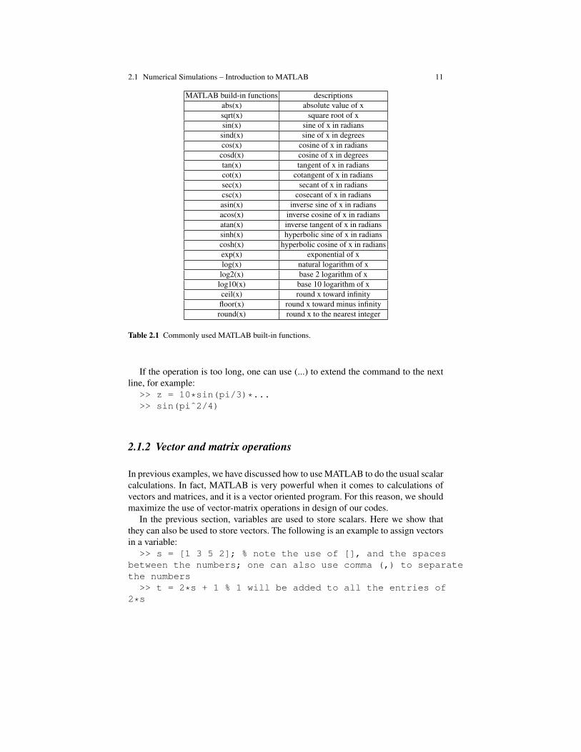
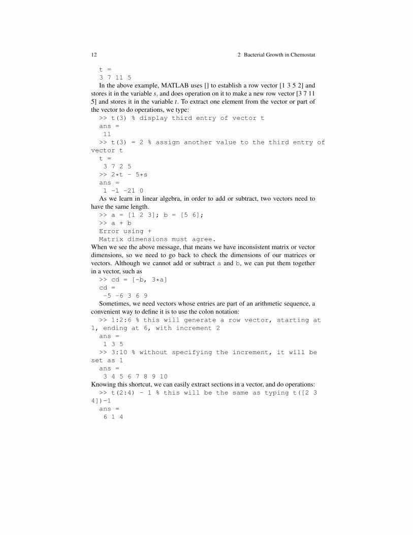
MATLAB has some built-in trigonometric function and elementary functions.We choose some commonly used ones to list in Table 2.1.
It is convenient and important to make comments in the codes, for future refer-ence. In MATLAB, we use the percentage sign (%), and MATLAB will take all thecharacters after (%) as comments and those will not be executed, for example: >> x= (5*2+3.5) / 5ˆ2 % store the result in variable z, and showthe result on the screen.
2.1 Numerical Simulations – Introduction to MATLAB 11
MATLAB build-in functions descriptionsabs(x) absolute value of xsqrt(x) square root of xsin(x) sine of x in radianssind(x) sine of x in degreescos(x) cosine of x in radianscosd(x) cosine of x in degreestan(x) tangent of x in radianscot(x) cotangent of x in radianssec(x) secant of x in radianscsc(x) cosecant of x in radiansasin(x) inverse sine of x in radiansacos(x) inverse cosine of x in radiansatan(x) inverse tangent of x in radianssinh(x) hyperbolic sine of x in radianscosh(x) hyperbolic cosine of x in radiansexp(x) exponential of xlog(x) natural logarithm of xlog2(x) base 2 logarithm of xlog10(x) base 10 logarithm of xceil(x) round x toward infinityfloor(x) round x toward minus infinityround(x) round x to the nearest integer
Table 2.1 Commonly used MATLAB built-in functions.
If the operation is too long, one can use (...) to extend the command to the nextline, for example:
>> z = 10*sin(pi/3)*...>> sin(piˆ2/4)
2.1.2 Vector and matrix operations
In previous examples, we have discussed how to use MATLAB to do the usual scalarcalculations. In fact, MATLAB is very powerful when it comes to calculations ofvectors and matrices, and it is a vector oriented program. For this reason, we shouldmaximize the use of vector-matrix operations in design of our codes.
In the previous section, variables are used to store scalars. Here we show thatthey can also be used to store vectors. The following is an example to assign vectorsin a variable:
>> s = [1 3 5 2]; % note the use of [], and the spacesbetween the numbers; one can also use comma (,) to separatethe numbers
>> t = 2*s + 1 % 1 will be added to all the entries of2*s
12 2 Bacterial Growth in Chemostat
t =3 7 11 5In the above example, MATLAB uses [] to establish a row vector [1 3 5 2] and
stores it in the variable s, and does operation on it to make a new row vector [3 7 115] and stores it in the variable t. To extract one element from the vector or part ofthe vector to do operations, we type:
>> t(3) % display third entry of vector tans =11>> t(3) = 2 % assign another value to the third entry of
vector tt =3 7 2 5>> 2*t - 5*sans =1 -1 -21 0
As we learn in linear algebra, in order to add or subtract, two vectors need tohave the same length.
>> a = [1 2 3]; b = [5 6];>> a + bError using +Matrix dimensions must agree.
When we see the above message, that means we have inconsistent matrix or vectordimensions, so we need to go back to check the dimensions of our matrices orvectors. Although we cannot add or subtract a and b, we can put them togetherin a vector, such as
>> cd = [-b, 3*a]cd =-5 -6 3 6 9
Sometimes, we need vectors whose entries are part of an arithmetic sequence, aconvenient way to define it is to use the colon notation:
>> 1:2:6 % this will generate a row vector, starting at1, ending at 6, with increment 2
ans =1 3 5
>> 3:10 % without specifying the increment, it will beset as 1
ans =3 4 5 6 7 8 9 10
Knowing this shortcut, we can easily extract sections in a vector, and do operations:>> t(2:4) - 1 % this will be the same as typing t([2 3
4])-1ans =6 1 4

2.1 Numerical Simulations – Introduction to MATLAB 13
We have learned how to define and use row vectors, and the operations are similarfor column vectors. The only difference is that the entries of a column vector areseparated by semicolon (;) or making a new line.
>> cv = [-1; pi; exp(2)]cv =1.00003.14167.3891>> cv2 = [123]cv2 =123
The row and column vectors can be transposed to become column and row vec-tors, respectively.
>> cv’, t’ans =1.0000 3.1416 7.3891ans =3725
Similarly to making vectors, users can make a m× n matrix, by adding a semi-colon ; after the end of each row. Next we define matrices. Similar to row and col-umn vectors, entries in a row are separated by spaces or commas, while differentrows are made by using semicolon or a new line. For example:
>> A = [1 2 3 4; 5 6 7 8; 9 10 11 12]A =1 2 3 45 6 7 89 10 11 12
We can extract or change any single entry in the matrix>> A(2,3) = 5; % change the (2,3) entry of A to 5
or extract part of the matrix>> B = A(2,1:3) % take the second row, the first to third
column, store as a new matrix B>> B =>> 5 6 7We can combine matrices, as long as the dimensions are consistent. >> A =[A
B’] % transpose B, make it as the last column vector andmerge with A
A =

14 2 Bacterial Growth in Chemostat
1 2 3 4 55 6 7 8 69 10 11 12 7
We can extract the whole row or colon by using semicolon>> A(:,3)A =3711
>> A(1,:)A =1 2 3 4 5
Then we can redefine or delete a row or a column:>> A(:,2) = [] % delete the second row of A (: represents
all the rows, [] is an empty vector>> A = [A; 4 3 2 1; 0 -1 -2 -3]; % adding the fourth and
fifth row in the matrix ATo obtain the size of a matrix, we use the command “size”.>> size(A’)ans =4 5
To obtain the length of a vector, we use “length”.>>length(A(1,:))ans =4
There are some built-in special matrices,>> ones(2,3) % this generates a 2x3 matrix with ones>> zeros(4,4) % this generates a 4x4 matrix with zeros>> eye(5) % this generates a 5x5 identity matrix>> diag([1 3 5]) % this generates a matrix with 1 3 5 on
its diagonalNext, let us about matrix-matrix or matrix-vector multiplication. When we use
* in the matrix operations, it will operates as the matrix multiplication, what welearned in linear algebra. For example,
>> X = [1 2 3; 0 2 4]; Y = [5 2; 1 1; 10 7]; W = X*YW =37 2542 30
If we try>> X*X
then we will see an error message about the matrix dimension, because an m× nmatrix can only by multiplied by an n× k matrix. Sometime we do not performcomponent-by-component operations, but not matrix-matrix multiplications, forthat purpose we need to use .* instead of *. The following commands will givedifferent result:
>> W.* W % component by component operation
2.1 Numerical Simulations – Introduction to MATLAB 15
>> W* W % matrix-matrix multiplicationand we will find that X.*Xworks because it is component-by-component operation.
2.1.3 Numerical algorithms of solving ODE
Most of the time, the solution of an ODE problem does not have a closed-formsolution. In this case, one looks for numerical solutions that approximate the realsolution. Since numerical solutions are just approximations, it is important to un-derstand the accuracy of the numerical method and robustness of it.
Suppose a scalar ODE is
dydt
= f (y, t) y(0) = y0, t ≥ 0.
Let t0 be some time point with t0 ≥ 0, then by integrating the ODE, one gets
y(t) = y(t0)+∫ t
t0f (x,τ)dτ ≈ y(t0)+(t− t0) f (y(t0), t0).
As long as t is sufficiently close to t0, this provides a good approximation. Define has the step size, we then define the numerical solution by
Yn+1 = Yn +h f (Y (tn), tn).
This is call forward Euler Method, named after Leonhard Euler (1707-1783). Theerror of this scheme is O(h), which can be formally derived from Taylor expansion.Generally, a numerical scheme is called kth order accurate if the error is O(hk),where h is the discretization size. Therefore, Euler method is first order accurate.Nowadays, there are many high order accurate schemes to solve ODE, but Eulermethod is still a classical one as one first learn numerical methods. We will revisitthe details about Euler methods in Chapter 6. In MATLAB, we have some optionsof using Runge-Kutta methods to solve ODE systems, which will be introduced inthe following.
Using MATLAB to solve ODE
When solving ODE with MATLAB, we need to represent f (y, t) as a “FUNCTION”in MATLAB, with the input t and y, and output dy. If we call teh FUNCTION file as“odefile.m”, the format of ODE is as follows: [t,y]=solver(’odefile’,[t0,t1],y0),where [t0, t1] is the time interval of interest, and y0 is the initial conditions. The op-tions for the solver can be found be look up “help” in MATLAB. For example:
>>[t,y]=ode45(’odefile’,[1,3],2)
16 2 Bacterial Growth in Chemostat
The above solves ODE with the prescibed f (y, t) in odefile.m, within the timerange [0,1] and initial data y(1) = 2. Let us find out what is in that file:
>> type odefile.mfunction dy = odefile(t,y)dy = yˆ2 + t;
Problem 2.6. Try the following command to generate a vector x.
>> x = 0:0.01:2What is x , explain what you see in MATLAB. Then use the command>> y = sin(x)to generate another vector y, what is y?Using the above commands to plot the figure of f (x) = 2sinx2 for 0 ≤ x ≤ 3,
with x incremented by 0.05 in the discretization.
Problem 2.7. Write a code to solve the ODE
dNdt
= N(
1− N2
), 0≤ t ≤ 5,
with initial condition N(0) = 0.5. Plot the numerical solution and the exact solutionon the same figure with different markers and different colors (refer to the numericalsection of Chapter 3 for plotting).
Problem 2.8. Solve the equation in Problem 2.5 with a = 1 numerically in the formx = x(t) when (i) x(0) = 1
2 , (ii) x(0) = 32 .
Chapter 3Linear Differential Equations
In order to use mathematics to answer biological questions we need to develop fur-ther the theory of differential equations. In this chapter we introduce linear differ-ential equations of the second order, and a system of two first-order differentialequations.
Consider a second order differential equation
ad2xdt2 +b
dxdt
+ cx = 0 (3.1)
where a, b, c are real constants and a 6= 0. The general solution is
x(t) = c1eλ1t + c2eλ2t , c1,c2 are constants, (3.2)
where λ1,λ2 are the solutions of the quadratic equation
aλ2 +bλ + c = 0,
namely,
λ1,2 =12a
(−b±√
b2−4ac) (3.3)
provided λ1 6= λ2. If λ1 = λ2 =− b2a , then teλ 1t is another solution of (3.1), and the
general solution of (3.1) is
x(t) = c1eλ1t + c2teλ1t . (3.4)
We can use the general solution to solve Eq. (3.1) subject to initial conditions
x(0) = α, x′(0) = β . (3.5)
Problem 3.1. Consider the equation (3.1) with initial conditions (3.5). Prove thatthere is a unique solution of the form (3.2) if λ1 6= λ2, and of the form (3.4) ifλ1 = λ2.
17

18 3 Linear Differential Equations
If b2−4ac is negative, then λ1 and λ2 are complex numbers,
λ1,2 =1
2a(−b± i
√4ac−b2) = µ± iν (3.6)
andeλ1,2t = eµt(cosνt± isinνt).
Then the general solution can be written in the form
x(t) = c1eµt cosνt + c2eµt sinνt.
Consider next a 2×2 linear system
dx1dt = a11x1 +a12x2
dx2dt = a21x1 +a22x2
(3.7)
We try to solve it in the form
x1 = v1eλ t , x2 = v2eλ t .
Then
a11v1 +a12v2 = v1λ
a21v1 +a22v2 = v2λ .
We can rewrite this system in matrix form(a11−λ a12
a21 a22−λ
)(v1v2
)=
(00
), (3.8)
or (A−λ I)v = 0 where
A =
(a11 a12a21 a22
), I =
(1 00 1
), v =
(v1v2
).
A nonzero solution v exists if and only if λ satisfies the characteristic equation
det(A−λ I) = 0. (3.9)
A solution λ of (3.9) is called an eigenvalue of A and a corresponding v is calledeigenvector. Eq. (3.9) can be written explicitly as
λ2−λ (a11 +a22)+(a11a22−a12a21) = 0. (3.10)
If the two eigenvalues λ1,λ2 are different, then the general solution of Eq. (3.7)is
x(t) = c1w1eλ1t + c2w2eλ2t , (3.11)

3 Linear Differential Equations 19
where w1 and w2 are the eigenvectors corresponding to λ1 and λ2, respectively.More precisely,
Theorem 3.1. If λ1 6= λ2 then for any initial values
x(0) = b where b =
(b1b2
), (3.12)
there is a unique solution of (3.7), (3.12) in the form (3.11).
Proof. We first claim that w1,w2 are linearly independent, that is,
if α1w1 +α2w2 = 0, then α1 = α2 = 0.
Indeed this relation implies that
α1λ1w1 +α2λ2w2 = α1Aw1 +α2Aw2 = A(α1w1 +α2w2) = 0.
Since also α1w1 +α2w2 = 0, we get, by subtraction,
α2λ2w2−λ1α2w2 = 0, or (λ2−λ1)α2w2 = 0.
If follows that α2 = 0, and then also α1 = 0.Setting
w1 =
(v11v12
), w2 =
(v21v22
)we conclude that
if2
∑i=1
vi jαi = 0 for j = 1,2, then α1 = α2 = 0.
Hence, det(vi j) = 0. But then, by linear algebra, for any (b1,b2) there is a uniquesolution (c1,c2) of the system
2
∑i=1
vi jci = bi ( j = 1,2),
and the function x(t) in (3.11) is the solution asserted in the theorem.
Consider now the case where λ1 is a complex number, λ1 = µ + iν . Then thecomponents of the eigenvector w1 are also complex numbers. But we are interestedonly in real-valued solutions. So in order to construct real-valued solutions we write
w1eλ1t =
(v11 + iv12v21 + iv22
)eµt(cosνt + isinνt) (3.13)
where vi j are real numbers. We note that the complex conjugate of w1eλ1t is also asolution of (3.7) and, hence, so are the real and imaginary parts of (3.13). It follows

20 3 Linear Differential Equations
that
eµt(
v11 cosνt− v12 sinνtv21 cosνt− v22 sinνt
)and eµt
(v11 sinνt + v12 cosνtv21 sinνt + v22 cosνt
)(3.14)
are two solutions.
Problem 3.2. Prove that the two solutions in (3.14) are linearly independent.
From Problem 3.2 it follows, as in the proof of Theorem 3.1, that any solution of(3.7) is a linear combination of the two solutions in (3.14).
By writing the roots λ1,λ2 of (3.10) in the form (3.3) or (3.6), we see that Reλ1 <0 and Reλ2 < 0 if and only if
trace of A≡ a11 +a22 < 0,determinant of A≡a11a22−a12a21 > 0. (3.15)
If λ1 = λ2, then in addition to a solution w1eλ1t of Eq. (3.7) where w1 is aneigenvector of (3.8) there is another solution of the form w1teλ t + w2eλ t where w2is an appropriate vector. Setting w2 = w1 + w2, the general solution of Eq. (3.7) is
x(t) = c1w2eλ1t + c2w1teλ1t .
Set x = (x1,x2). The proint x = 0 is called an equilibrium point of (3.7), sincethe solution x(t) with x(0) = 0 is x(t)≡ 0. We define the phase space for Eqs. (3.7)as the (x1,x2)-space, and we want to draw the portrait of the trajectories in this spacenear x = 0, at least qualitatively. This can be done with the aid of the form (3.11) ofthe general solution. The protrait will depend on the eigenvalues λ1,λ2 as follows.
Figures 3.1(B) and 3.1(E) show that when both eigenvalues have negative realparts, all the trajectories converge to x = 0; we say that x = 0 is a stable equilibrium(or more precisely, asymptotically stable equilibrium). On the other hand, when atleast one of the eigenvalues has positive real part, there are always trajectories thatgo away from x = 0 even if they start initially near x = 0; we say that x = 0 is anunstable equilibrium.
In order to solve an inhomogeneous linear equation
ad2xdt2 +b
dxdt
+ cx = f (t) (3.16)
with a given function f (t), we first find a special solution x(t) and, then, the generalsolution is a sum of x(t) and the general solution of the homogeneous equation. Thesame procedure applies to inhomogeneous linear systems.
Problem 3.3. Find the general solution of x′′+ x′− x = t2.
Problem 3.4. Find the solution of x′′−4x′+3x = e−t with x(0) = 18 ,x′(0) = 1
4 .

3.1 Numerical Simulations 21
Fig. 3.1 Phase portrait
Problem 3.5. Find the general solution of
dx1
dt= −2x1 +7x2
dx2
dt= 2x1 +3x2.
Problem 3.6. Find the general solution of
dx1
dt= x1−2x2
dx2
dt= 2x1 + x2.
3.1 Numerical Simulations
3.1.1 Solving a second order ODE
In previous chapters, we have simulated scalar first order ODEs with MATLAB. Anatural question is that whether we need additional MATLAB functions to simulate

22 3 Linear Differential Equations
higher oder equations? The answer is no. What we need to do is to convert higherorder equations into systems of ODEs, and then we will simulate the ODE systems.Let’s take a second order ODE as an example:
u′′(t)+16u
′(t)+192u(t) = 0
can be converted to {x′1 = x2
x′2 = −16x2−192x1
by letting x1 = u and x2 = u′. In general, a system of two first order ordinary differ-ential equations has the form {
x′1 = F1(x1,x2, t)
x′2 = F2(x1,x2, t)
(3.17)
For example, given an ODE system
ddt
(x1x2
)=
(1 22 3
)(x1x2
)+
(0t2
), 0≤ t ≤ 1,
with initial condition(
x1(0)x2(0)
)=
(23
), we can solve with MATLAB as follows.
First, we create the main script file, named main.m, in which we typex ini = [2,3]’;[t,x] = ode45(’odefile’, [0,1], x ini); This file is the file we
execute in MATLAB, which may call other functions. Now we have defined theinitial condition, and we need to define F1(x1,x2, t) and F2(x1,x2, t). To do that, wecreate another script file called define.m, which is a function file that will be calledwhile MATLAB is running ode45. In odefile.m, we type
function dx = odefile(t,x)A = [1,2; 2,3];dx = A*x + [0, tˆ2]’;
By running main.m, we end up with MATALB variables t and x, which are columnvectors. Variable t has components as the discrete time that MATLAB uses to in thesimulation, and the components of x are approximated values for the correspondingcomponent in t.
3.1.2 Plotting figures
Suppose x = [x1,x2,x3, · · · ,xn] is a vector representing sampling points on x−axisand y = [y1,y2,y3, · · · ,yn] represents the corresponding function values of compo-nents of x (note that x and y must be of the same length), then to plot x versus y, oneuses

3.1 Numerical Simulations 23
>> plot(x,y)To label the axis, we can use>> xlabel(’x’), ylabel(’y’)One can also specify the color and marker by addtng an option in the “plot”
function>> plot(x,y,’r o’) % this marks those point values by red
circlesIf we would like to overlay two curves, x versus y and x versus z, where z =
[z1,z2,z3, · · · ,zn], we can use>> plot(x,y,’r’,x,z,’b’) % mark the first y(x) function
in red and the second z(x) in blue.or>> plot(x,y,’r’), hold on>> plot(x,z,’b’)The “hold on” command holds the first figure data and the second will be plotted
on top of the first one. Without this command, the previous data in the figure will beoverwritten.
Problem 3.7. (a) Rewrite Problem 3.4 into first order systems. (b) Take the initialcondition to be x(0) = 1,x′(0) = 0, and the time interval 0 ≤ t ≤ 3. Use MATLABto solve the system you get in (a), and plot the two variables on the same figure.
Problem 3.8. Solve y′′− 5y′ = 0, y(0) = 1, y′(0) = 2, first explicitly, and then nu-merically. Compare the two graphs of y(t) for 0≤ t ≤ 3.
Problem 3.9. Solve
dx1
dt= x1− x2
dx2
dt= x1 + x2
with x1(0) = 1,x2(0) = 5, first explicitly and then numerically and compute the twographs of x1(t) for 0≤ t ≤ 2.


Chapter 4Systems of two differential equations
The system (3.7) is linear. In this chapter we study general systems of two differen-tial equations has the form
dx1
dt= f1(x1,x2),
dx2
dt= f2(x1,x2), (4.1)
where f1(x1,x2), f2(x1,x2) are any given functions, not necessarily linear. A point(a,b) such that
f1(a,b) = 0, f2(a,b) = 0
is called an equilibrium point, a stationary point or a steady point of the system(4.1). The x1-nullcline of (4.1) is the curve consisting of points satisfying the equa-tion
f1(x1,x2) = 0.
Similarly, the x2-nullcline is the curve defined by
f2(x1,x2) = 0.
The equilibrium points of the system (4.1) are the points where the two nullclinesintersect. To get an idea how trajectories behave near a stationary point (a,b), welinearize the system.
We setX1 = x1−a, X2 = x2−b.
Then, by Taylor’s formula,
fi(x1,x2) = fi(a+X1,b+X2) = fi(a,b)+∂ fi
∂x1X1 +
∂ fi
∂x2X2 + small terms,
where∂ fi
∂x1=
∂ fi
∂x1(a,b),
∂ fi
∂x2=
∂ fi
∂x2(a,b).
If we define
25
26 4 Systems of two differential equations
ai j =∂ fi
∂x j(a,b)
then the system (4.1) near (a,b) has the form
dXi
dt= ai1X1 +ai2X2 + small terms (i = 1,2)
when X1,X2 are near 0. Hence the trajectories of (4.1) are expected to behave ap-proximately like the trajectories of
dXi
dt= ai1X1 +ai2X2, i = 1,2. (4.2)
Accordingly, the equilibriun point (a,b) of (4.1) is said to be stable if the equi-librium point x = 0 of (4.2) is stable, that is, if the real parts of eigenvalues of thematrix A = (ai j) are negative.
We conclude that the equilibrium point (a,b) of the system (4.1) is stable if andonly if the following inequalities hold at (a,b):
∂ f1∂x1
+ ∂ f2∂x2
< 0,∂ f1∂x1
∂ f2∂x2− ∂ f1
∂x2
∂ f2∂x1
> 0.(4.3)
i.e., trace of(
∂ fi∂x j
)< 0 and determinant of
(∂ fi∂x j
)> 0. The matrix ( ∂ fi
∂x j(a,b)) is
called the Jacobian matrix at the equilibrium point (a,b).
Problem 4.1. The system
dxdt
= x2− y2
dydt
= x(1− y)
has two nonzero equilibrium points (1,1),(−1,1). Find the eigenvalues of the Jaco-bian matrix for each of these points, and determine the behavior of the trajectoriesin terms of the classification described in the graphs in Fig. 3.1.
Problem 4.2. Do the same for the system
dxdt
= x− xy2,dydt
= y+ xy2 +1
with its steady points (0,−1),(−2,1).

4.1 Numerical Simulations 27
4.1 Numerical Simulations
As mentioned in the previous chapter. In general, a system of two first order ordinarydifferential equations has the form{
x′1 = F1(x1,x2, t)
x′2 = F2(x1,x2, t)
(4.4)
If it is a linear system, the general form can be written as{x′1 = a11(t)x1 +a12(t)x2 +b1(t)
x′2 = a21(t)x1 +a22(t)x2 +b2(t),
(4.5)
which can be written concisely as
x′ = A(t)x+b(t)
where
x =(
x1(t)x2(t)
),b(t) =
(b1(t)b2(t)
),A(t) =
(a11(t) a12(t)a21(t) a22(t)
)When A is a constant matrix and b = 0, the solution can be easily carried out via
eigenvalue and eigenfunction computation.Example 1:
x′=
(1 14 1
)x (4.6)
x = c1
(12
)e3t + c2
(1−2
)e−t
The origin is a saddle point and is unstable (Figure 4.1).
Fig. 4.1 Unstable saddle point.

28 4 Systems of two differential equations
In MATLAB, this is a simple one-line command to compute eigenvalue andeigenvector.
>> A=[1 1;4 1];>> [V,D]=eig(A)V =0.4472 -0.44720.8944 0.8944D =3.0000 0 0 -1.0000Example 2:
x′=
(−3√
2√2 −2
)x
x = c1
(1√2
)e−t + c2
(−√
21
)e−4t
The original is a stable node (Figure 4.2). (Figure 4.1).
Fig. 4.2 Stable saddle point.
Example 3:
x′=
(− 1
2 1−1 − 1
2
)x
x = c1
(cos(t)−sin(t)
)e−t/2 + c2
(sin(t)cos(t)
)e−t/2
The origin is a spiral point and is asymptotically stable (Figure 4.3).Example 4:
x′=
(1 −11 3
)x

4.1 Numerical Simulations 29
Fig. 4.3 Stable spiral.
x = c1
(1−1
)e2t + c2
[(1−1
)te2t +
(0−1
)e2t]
Fig. 4.4 Unstable steady state.
The origin is an improper mode, and is unstable (Figure 4.4).
Problem 4.3. Give a 2 by 2 linear system that the origin is (a) unstable node, realeigenvalues and λ1 > 0, λ2 > 0 (b) stable node, real eigenvalues and λ1 < 0, λ2 < 0(c) saddle point, real eigenvalues and λ1λ2 < 0 (d) unstable spiral, complex eigen-values λ = α + iβ and α > 0 (e) stable spiral, complex eigenvalues λ = α + iβand α < 0 (f) center, λ = α + iβ and α = 0. For all the above systems, plot thedirectional fields for −3≤ x≤ 3,−3≤ y≤ 3.

30 4 Systems of two differential equations
Problem 4.4. Solve numerically
x = xy− y, y = xy+ x
with x(0) = 1, y(0) = 1, for 0≤ t ≤ 3.
Problem 4.5. Solve numerically
x = x− xy2, y = y+ xy2 +1
with x(0) = 1, y(0) = 1, for 0≤ t ≤ 3.
Problem 4.6. 3.6. Solve numerically
x =−xy, y = (1− x)(1+ y)
with x(0) = 2, y(0) = 0, for 0≤ t ≤ 4.
Chapter 5Predator-Prey Models
A predator is an organism that eats another organism. A prey is an organism that apredator eats. In ecology, a predation is a biological interaction where a predatorfeeds on a prey. Predation occurs in a wide variety of scenarios, for instance inwild life interactions (lions hunting zebras, foxes hunting rabbits), in herbivore-plantinteractions (cows grazing), and in parasite-host interactions.
If the predator is to survive over many generations, it must ensure that it con-sumes sufficient amount of prey, otherwise its population will decrease over timeand will eventually disappear. At the same time the predator must not over-consumethe prey, for if the prey population will decrease and disappear, then also the preda-tors will die out, from starvation.
Thus the question arises: what is the best strategy of the predator that will ensureits survival. This question is very important to ecologists who are concerned withbiodiversity. But it is also an important question in the food industry; for example,in the context of fishing, what is the sustainable amount of fish harvesting?
In this chapter we use mathematics to provide answers to these questions.We begin with a simple predator-prey example.We denote by x the density of a prey, that is, the number of prey animals per unit
area on land (or volume in sea) and by y the density of predators. We denote by athe net growth rate in x (birth minus natrual death), and by c the net death rate ofpredators. The growth of predators is assumed to depend only on the prey as food.Predation occurs when predator comes into close contact with prey, and we take thisencounter to occur at an average rate b. Hence
dxdt
= ax−bxy. (5.1)
The growth of predators is proportional to bxy, so that
dydt
= dxy− cy. (5.2)
In terms of dimensions,
31

32 5 Predator-Prey Models
[a] =1
time, [b] =
1density of predator
1time
,
and[c] =
1time
, [d] =1
density of prey1
time.
The system (5.1), (5.2) has two equilibrium points. The first one is (0,0); thiscorresponds to a situation where both species die. This equilibrium point is unstable.Indeed the Jacobian matrix at (0,0) is(
a 00 −c
)and one of the eigenvalues, namely a, is positive.
The second equilibrium point is ( cd ,
ab ) and the Jacobian matrix at this point is(0 −bc
dadb 0
)The corresponding eigenvalues are λ = ±i
√ac. According to Fig. 3.1 the phase
portrait is a circle. We conclude: The predator and prey can both survive forever,and their population will undergo periodic (seasonal) oscillations.
Eqs. (5.1), (5.2) are examples of what is known as Lotka-Volterra equations.One can introduce various variants into these equations. For example, if the preypopulation is quite conjested, we may want to use the logistic growth, and write
dxdt
= ax(1− xB)−bxy. (5.3)
More general models of predator-prey are written in the form
dxdt
= x f (x,y),dydt
= yg(x,y)
where x is the prey and y is the predator, ∂ f/∂y < 0,∂g/∂x > 0, and ∂ f/∂x < 0for large x, ∂g/∂y < 0 for large y. The first two inequalities mean that the preypopulation is depleted by the predator and the predator population is increased byfeeding on the prey. The last two inequalities represent natural death due to thelogistic growth model.
We next consider a plant-herbivore model. The herbivore N feeds on plant P. Wetake the consumption rate of the plant to be
σP1+P
N;
this means that, at small amount of P, N consumes P at a linear rate σP, but the rateof consumption by N is limited and cannot exceed σN. Thus,

5 Predator-Prey Models 33
dPdt
= rP−σP
1+PN. (5.4)
The equation for the herbivore is
dNdt
= λσP
1+PN−dN. (5.5)
Here d is the death rate of N, and λ is the yield constant, that is,
λ =mass of herbivore formed
mass of plant used;
naturally λ < 1. Note that if λσ < d then dNdt < 0 and the herbivore will die out.
Problem 5.1. Show that in the model (5.2), (5.3), if B > cd then the point (x,y) =
( cd ,
ab (1−
cBd )) is a stable equilibrium point.
In both models (5.1), (5.2) and (5.3), (5.2), the consumption rate of the prey bythe predator is proportional to the density of the prey. In both models the predatorand prey co-exist, either as stable steady state for model (5.3), (5.2) and as periodicsolution for model (5.1), (5.2). The situation is quite different for the model model(5.4), (5.5), since the herbivore consumption is not proportional to the density of theplant, but is rather limited by the parameter σ . In this case, since (0,0) is unstableequilibrium, we expect herbivore and plant to co-exist but their dynamics is quitecomplicated.
We conclude that if the prey undergoes logistic growth then the populations ofpredator and prey will survive and stabilize at fixed levels, rather than survive withseasonal oscillation (as was the case in the model (5.1), (5.2)).
Factorization rule
Consider a system (4.1) where the fi can be factored as follows:
f1(x1,x2) = x1g1(x1,x2), f2(x1,x2) = x2g2(x1,x2),
so thatdx1
dt= x1g1(x1,x2),
dx2
dt= x2g2(x1,x2)
In this case there are equilibrium points P1 = (0,0),P2 = (0, x2) if g2(0, x2) = 0,P3 = (x1,0) if g1(x1,0) = 0, and P4(x1, x2) if g1(x1, x2) = 0, g2(x1, x2) = 0. We canthen quickly compute the Jacobian matrix J(Pi) at each point Pi. For example, tocompute J(P4) when x1 > 0, x2 > 0, we notice that since g1 = g2 = 0 at P4,
J(P4) =
(x1
∂g1∂x1
x1∂g1∂x2
x2∂g2∂x1
x2∂g1∂x2
)(x1,x2)
.
34 5 Predator-Prey Models
Similarly,
J(P1) =
(g1(0,0) 0
0 g2(0,0)
),
J(P2) =
(g1 0
x2∂g2∂x1
x2∂g1∂x2
)(0,x2)
and
J(P3) =
(x1
∂g1∂x1
x1∂g1∂x2
0 g2
)(x1,0)
where x1 > 0.
We shall refer to these shortcuts in the computation of the Jacobian matrix as thefactorization rule.
Use the factorization rule to solve Problems 5.2, 6.3.
Problem 5.2. Show that in the plant-herbivore model (5.4)-(5.5), the equilibriumpoint (0,0) is unstable.
Problem 5.3. Assume that in the model (5.4)-(5.5), λσ > d. Prove that there is asecond equilibrium point (P2,N2) where
P2 =d
λσ −d, N2 =
λ rλσ −d
, (5.6)
and that it is unstable.
The Allee effect refers to the biological fact that increased fitness correlates pos-itively with higher population, or that “undercrowding” decreases fitness. Morespecifically, if the size of a population is below a threshold then it is destined forextinction. Endangered species are often subject to the Allee effect.
Consider a predator-prey model where the prey is subject to the Allee effect,
dxdt
= rx(x−α)(1− x)−σxy, (0 < α < 1), (5.7)
that is, if the population x(t) decreases below the threshold x = α , then x(t) willdecrease to zero as t→ ∞. The predator y satisfies the equation
dydt
= λσxy−σy (5.8)
where λ is the yield constant. The point (0,0) is an equilibrium point of the system(6.14)-(6.15).
Problem 5.4. Show that if α < δ
λσ< 1, then the system (6.14)-(6.15) has a second
equilibrium point (x, y) = ( δ
λσ,r( δ
λσ−α)(1− δ
λσ)), and it is stable if
δ
λσ>
1+α
2.

5.1 Numerical Simulations 35
This result shows that for the predator to survive, the prey must be allowed tosurvive, and the predator must adjust its maximum eating rate, σ , so that
δ
λ< σ <
δ
λ
21+α
.
If the Allee threshold, α , deteriorates and approaches 1, the predator must thendecrease its rate of consumption of the prey and bring it closer to δ/λ , otherwise itwill become extinct.
5.1 Numerical Simulations
The following algorithms code (5.1)-(5.2). These codes also demonstrate how to im-plement nonlinear systems (see fun predator prey.m). Also note that in model predator prey.m,when we plot both x and y variables, we use “subplot” command. The “subplot” al-lows one to plot more than one subfigures in one plot. Its argument (m,n,k) standsfor total number of rows, total number column and the place of the subfigurem re-spectively. You can type
>> help subplotto see how to use it.
Algorithm 1 model predator prey.m% This code simulates model (5.1)-(5.2).close all,clear all,% define global parametersglobal a b c d% starting and final timet0 = 0; tfinal = 5;% paramtersa = 5; b = 2; c = 9; d = 1;% initial conditionsv0 = [10,5];[t,v] = ode45(’fun predator prey’,[t0,tfinal],v0);subplot(1,2,1)plot(t,v(:,1)) % plot the evolution of xxlabel t, ylabel xsubplot(1,2,2)plot(t,v(:,2)) % plot the evolution of yxlabel t, ylabel y
Problem 5.5. Plot the time evolution of model of equations (5.1)-(5.2) with a =5,b = 2,c = 9,d = 1 starting from (10,5), for time from 0 to 5.

36 5 Predator-Prey Models
Algorithm 2 fun predator prey.m% This is the function file called by model predator prey.mfunction dy = ffun predator prey(t,v)global a b c ddy = zeros(2,1);dy(1) = a*v(1) - b*v(1)*v(2);dy(2) = -c*v(2) + d*v(1)*v(2);
Problem 5.6. Draw the phase portrait for (5.1), (5.2) with a = 5,b = 2,c = 9,d = 1starting from several points near (9,5/2).
Problem 5.7. The only nonzero steady point of (5.2), (5.3) is ( cd ,
ab −
acbdB ); it is
biologically meaningful only if 1− cdB > 0, and it is a stable spiral. Draw several
trajectories when a = b = c = d,B = 2.
Problem 5.8. Draw the phase diagram for (5.2), (5.3) in case a = b = c = d,B = 12 .
Problem 5.9. Change the codes (adding one more global parameter B, and changedy(1) in fun predator prey.m) to implement (5.2)-(5.3). Plot the time evolutionwitha = 5,b = 5,c = 5,d = 5,B = 0.5 starting from (2,3), for time from 0 to 5.

Chapter 6Two competing populations
Competition is an interaction between organisms, or species, sharing resources thatare in limited supply. This is an important topic in ecology. The ‘competitive ex-clusion principle’ asserts that species less suited to compete will either adapt or dieout. In aggressive competition one species may attempt to kill the other. This situ-ation occurs, for example, among some species of ants, and some species or yeast.When enough data is known about the history of a specific competition between twospecies, mathematics can then be used to predict whether both species will surviveand co-exist or whether one of them will die out.
In this chapter we consider some examples of competing populations and deter-mine, using mathematics, whether one or both species will survive. We begin withthe following model:
dxdt
= r1x(1− xk1)−b1xy, (6.1)
dydt
= r2x(1− yk2)−b2xy, (6.2)
In Eq. (6.1), r2 is the growth rate of species x, k1 is the carrying capacity whichlimits its growth, and b1 is the rate by which the competitor y kills x. Eq. (6.2) hassimilar interpretation.
The system (6.1)-(6.2) has equilibrium points
(0,0), (k1,0), (0,k2). (6.3)
Note that the equilibrium point (k1,0) means that the second population becomesextinct. Similarly, (0,k2) corresponds to a situation where the first population be-comes extinct.
In order to determine whether there exist additional equilibrium points, we mustsolve the equations
37
38 6 Two competing populations
r1(1−xk1)−b1y = 0,
r2(1−yk2)−b2x = 0.
The solution is given by
(β1k2− k1
β1β2−1,
β2k1− k2
β1β2−1) where βi =
kibi
ri, (i = 1,2). (6.4)
This steady point is of biological relevance only if the two components are posi-tive, which occurs only when either
k1 >r2
b2, k2 >
r1
b1
ork1 <
r2
b2, k2 <
r1
b1.
Problem 6.1. Determine whether the equilibrium points in (6.3) are stable.
Problem 6.2. Show that the steady point defined in (6.4) is the unique equilibriumpoint (x,y) of (6.1) with x 6= 0,y 6= 0, and show that it is stable if k1 <
r2b2
and k2 <r1b1
.
The result means that both species will co-exist provided that rate of killing byb j is less than the rate ri/ki of growth rate divided by the carrying capacity, forj = 1, i = 2 and for j = 2, i = 1.
In the next example two species are competing for space. Consider for examplegrass (x) and weed (y) growing in the same field. They share some resources, e.g.,nutrients from the ground. But they also receive resources independently from eachother, e.g., sunshine and rain. Thus they only partially infringe upon each other interms of the medium carrying capacity which supports their growth. We can modeltheir dynamics as follows:
dxdt
= r1x(1− x+αyK
)−µ1x, (6.5)
dydt
= r2y(1− βx+ yK
)−µ2y, (6.6)
where 0 < α < 1,0 < β < 1. Assuming that r1 = r2 = r, µ1 = µ2 = µ and r > µ ,there is a steady state, (x, y), where they co-exist:
r(1− x+α yK
)−µ = 0,
r(1− β x+ yK
)−µ = 0.
Problem 6.3. Show that the steady state of co-existence is given by
6 Two competing populations 39
(K(1− µ
r )(1−α)
1−αβ,
K(1− µ
r )(1−β )
1−αβ).
and that this steady point is stable.
Problem 6.4. The model (6.5), (6.6) with α > 1,β > 1 represents the growth of twospecies under fierce competition for resources. In this case, the steady point of co-existence is given by the same expression as in Problem 6.3. Show that this steadystate is unstable.
The results of Problems 6.3 and 6.4 show that when two species are using thesame resources, they both will stably co-exist if they do not infringe significantlyupon each other, but they cannot stably co-exist if the competition is too aggressive.
Cancer model
Recall that logistic growth for a population with density x was modeled by
dxdt
= rx(1− xK)−µx
where r is the growth rate, µ is the death rate, and K is the medium carrying capacitywhich is determined by the resources available to support the population. If µ > rthen dx
dt +(µ− r)x≤ 0 so that
x(t)≤ x(i)e−(µ−r)t → 0, as t→ ∞.
We are interested in cases where populations persist, so we shall take µ < r.If two populations x and y co-exist in the same medium and follow a logistic
growth, then
dxdt
= r1x(1− x+ yK
)−µ1x,
dydt
= r2y(1− x+ yK
)−µ2y.
where r1 and r2 are the growth rates of the populations x and y, respectively, andµ1 and µ2 are their respective death rates. Note that the two population share themedium, hence the term (x+ y)/K represents the load of the total population x+ yon the medium carrying capacity K. We shall apply this model to cancer in a humantissue, where x represents the density of normal healthy cells and y represents thedensity of cancer cells in the same tissue. Since cancer cells proliferate faster thannormal healthy cells, we take
r2 > r1
. For simplicity we assume that µ1 = µ2 = µ . Writing
40 6 Two competing populations
dxdt
= x[r1(1−x+ y
K)−µ], (6.7)
dydt
= y[r2(1−x+ y
K)−µ], (6.8)
we observe that there cannot be a steady point (x, y) with x > 0, y > 0. On the otherhand there are steady points
((1− µ
r1)K,0), (0,(1− µ
r2)K).
Problem 6.5. Prove that (0,(1− µ
r2)K) is stable, and ((1− µ
r1)K,0) is unstable.
This result means that cancer-free state is unstable whereas the steady state whereall cells are cancer cells is stable.
It is interesting to explore the dynamics of the system (6.16), (6.8). We have
ddt
lnyx=
1y
dydt− 1
xdxdt
= (r2− r1)(1−x+ y
K). (6.9)
To make use of this formula we first show that if x(0) + y(0) < K then for anysufficiently small ε > 0 with x(0)+ y(0)+ ε < K, there holds:
x(t)+ y(t)< K− ε for all t > 0. (6.10)
Indeed, suppose this claim is not true, then there is a smallest t such that (6.10) holdsfor all t < t but
x(t)+ y(t) = K− ε. (6.11)
It follows thatddt(x(t)+ y(t))t=t ≥ 0. (6.12)
However, form Eqs. (6.16), (6.8) and (6.11), we get
ddt(x(t)+ y(t))t=t ≤ (K− ε)r1(1−
K− ε
K)−µx(t)
+(K− ε)r2(1−K− ε
K)−µy(t)
< K(r1 + r2)ε
K−µ(K− ε)< 0
if ε is sufficiently small, which is a contradiction to (6.12). Hence the assertion(6.10) is valid.
Substituting (6.10) into (6.9) we get
ddt
lnyx≥ (r2− r1)(1−
K− ε
K) =
(r2− r1)ε
K≡ δ .
It follows that

6.1 Numerical Simulations 41
lny(t)x(t)≥ ln
y(0)x(0)
+δ t
if y(0)> 0,x(0)> 0, so that, with C = y(0)/x(0),
y(t)x(t)≥Ceδ t .
But since, by (6.10), y(t)< K for all t > 0, we conclude that
x(t)≤ KC
e−δ t → 0, as t→ ∞. (6.13)
From (6.8) and (6.13) we deduce that if y(t)> (1− µ
r2)K and t is large, then dy(t)
dt < 0,
whereas if y(t)< (1− µ
r2)K and t is large then dy(t)
dt > 0. Hence y(t)→ (1− µ
r2)K as
t→ ∞.We have thus proved:
Theorem 6.1. The steady cancer-only state (0,(1− µ
r2)K) is globally asymptotically
stable.
Thus, the model (6.16), (6.8) predicts that, without treatment, the cancer cells willfill the entire tissue.
6.1 Numerical Simulations
6.1.1 Revisiting Euler method for solving ODE – consistency andconvergence
Suppose the system of ODEs we would like to solve is
dxdt
= f (x, t), t ≥ t0, x(t0) = x0 (6.14)
where f is a Lipschitz function in x and t and the initial condition x0 is a givenvalue in R. Note that even now we consider a single equation where x is a scalar, thediscussion in the following can be easily generalized to systems in which x and frepresent vectors. There are various ways to derive Euler method, here we give onederivation based on linear interpolation.
Integrating Eq. (6.14) from t1 to t1 +h, with t1 > t0, one abtains
x(t1 +h) = x(t1)+∫ t1+h
t1f (x(τ),τ)dτ.
If we approximate the integral by h f (x(t1), t1), which would be a good approxima-tion given h sufficiently small, then

42 6 Two competing populations
x(t1 +h)≈ x(t1)+h f (x(t1), t1).
Thus, we have the forward Euler method by denoting X j as the numerical solution attime tn, j = 1, · · · ,N, where tn are equi-distanced grid points with t0 < t1 < · · ·< tNand h = tn+1− tn,
Xn+1 = Xn +h f (Xn, tn). (6.15)
This type of scheme is call explicit scheme because the solution Xn+1 is explicitlydefined in function of Xn. In other words, knowing Xn, one can explicitly computeXn+1. Furthermore, it is called a single step method because it requires only solutionat one time step in order to compute the solution at the following time step.
In order to understand how good the numerical solution is, we define local trun-cation error to measure how closely the difference operator approximates the dif-ferential operator, for Euler method:
dn =x(tn+1)− x(tn)
h− f (x(tn), tn) =
h2
x′′(tn)+O(h2).
where tn is some point in the interval [tn, tn+1]. If a method has the local truncationerror O(hp), we say that the method is pth order accurate.
However, the real goal is not consistency but convergence. Assume Nh isbounded independent of N. The method is said to be convergent of order p ifthe global error en, where en = Xn− x(tn), e0 = 0, satisfies
en = O(hp), n = 1,2, · · · ,N.
Problem 6.6. Consider the scalar problem
y′ =−5ty2 +5t− 1
t2 , y(1) = 1.
(a) Verify that y(t) = 1t is a solution to the problem. (b) Use forward Euler method
until t = 10. Compute the error between the numerical solution and exact solutionusing h = 0.002,0.004,0.008,0.016. From the errors, what can you say about theorder of the scheme?
6.1.2 Backward Euler Method
While forward Euler method allows one to compute the numerical solution explic-itly, backward Euler method is an implicit method in which one may have to solvea system of nonlinear equations. Given the equation
dxdt
= f (x, t), t ≥ t0, x(t0) = x0,
6.1 Numerical Simulations 43
if we denote X j as the numerical solution at time tn, j = 1, · · · ,N, where tn are equi-distanced grid points with t0 < t1 < · · · < tN and h = tn+1− tn, the backward EulerMethod is
Xn+1 = Xn +h f (Xn+1, tn+1). (6.16)
Note that the difference between forward Euler and backward Euler is that we areusing unknown Xn+1 in function f of Eq. (6.16). To solve Eq. (6.16), one needs tosolve
Xn+1−h f (Xn+1, tn+1) = Xn,
which may require a nonlinear solver to solve this system. Recall that in the forwardEuler method, Xn+1 is directly computed from the right-hand-side using Xn.
Why would we want to use an implicit method which involves time consumingnonlinear solvers? The reason is “stability”. Consider the test equation y′ = λy, thebackward Euler for that equation is
Xn+1 = Xn +hλXn+1,
therefore(1−hλ )Xn+1 = Xn,
andXn+1 =
Xn
1−hλ.
Because we assume λ < 0, we have |Xn+1| < |Xn| regardless of the choice of h. Inother word, this scheme is stable for every h! We call this scheme “unconditionallystable”. This scheme is very useful if one requires a very small time step h to obtaina stable numerical solution with explicit scheme. In that case, solving nonlinearsystems will pay off by gaining stability.
Problem 6.7. Consider
dydt
=−10y, y(0) = 1, 0≤ t ≤ 3.
(i) Impliment backward Euler method, use h = 0.01,0.05,0.1,0.2. Compare thosesolutions with the exact solution. (ii) Use h = 0.21 in forward Euler and backwardEuler methods, and compare both numerical solutions with exact solutions in onefigure. (iii) Use h = 0.3 in forward Euler and backward Euler methods, what do yousee. Plot your numerical solutions if possible.
Problem 6.8. Implement the backward Euler method for
dydt
=−y+ t, y(0) = 1, 0≤ t ≤ 1.
Compare your numerical solution with the exact solution (you need to derive your-self).

44 6 Two competing populations
In MATLAB, there are also implicit methods that would efficiently and robustlycalculate stiff problems. The widely used function is called “ode15s”. Consider astiff problem
ddt
[x1x2
]=
[−1 −11 −5000
][x1x2
](6.17)
with initial conditions [x1x2
]=
[11
].
Problem 6.9. (a) Solve (6.8) with the initial condition with “ode45” in matlab. Com-pute the CPU time with “tic” and “toc”. (b) Repeat (a) with “ode15s”.

Chapter 7General systems of differential equations
In this chapter, we develop a theory for a system of differential equations that willbe used to study models with many species. We write the system either as
dxi
dt= fi(x1,x2, · · · ,xn), i = 1,2, · · · ,n (7.1)
or, in vector notation,dxdt
= f(x) (7.2)
where x = (x1, · · · ,xn), f = ( f1, · · · , fn).A point x0 = (x01, · · · ,x0n) such that f(x0) = 0 is called an equilibrium point, a
stationary point or a steady point, of the system (7.1). The unique trajectory x(t)with x(0) = x0 is then x(t)≡ x0, for all t ≥ 0.
Writing
fi(x) = fi(x0)+n
∑j=1
(x j−x j0)
[∂ fi
∂x j+ ε j(|x−x0|)
]where ε j(s)→ 0 if s→ 0, we see that the linear system of differential equations
dxi
dt=
n
∑j=1
ai j(x j− x j0), (ai j =∂ fi(x0)
∂x j) (7.3)
is a good approximation to (7.1) near x = x0. As in the analysis in Chapters 2 and3, we wish to determine under what conditions all solutions of (7.3) converge to x0as t→ ∞, and in this case we call x0 a stable equilibrium point, or, more precisely,asymptotically stable equilibrium point.
We try to find solutions of (7.3) in the form veλ t where v = (v1,v2, · · · ,vn). Thenλ and v must satisfy the equations
n
∑j=1
(ai j−λδi j)v j = 0, j = 1, · · · ,n (7.4)
45

46 7 General systems of differential equations
or, in matrix form,(J−λ I)v = 0 (7.5)
where I is the unit matrix, with elements δi j = 0 if i 6= j, δii = 1, and the matrix J isgiven by
J =
∂ f1∂x1
∂ f1∂x2· · · ∂ f1
∂xn...
∂ fn∂x1
∂ fn∂x2· · · ∂ fn
∂xn
where ∂ fi
∂x jis computed at x0; we also write J = ( ∂ fi
∂x j). The matrix J is called the
Jacobian matrix at x0.The system (7.4) has a solution v 6= 0 if and only if λ satisfies the equation
det(ai j−λδi j) = 0. (7.6)
This polynomial equation is called the characteristic equation, and the solutions λ
are called eigenvalues. A solution v of (7.5) is called an eigenvector correspondingto λ .
Equation (7.6) is a polynomial equation of order n,
λn +a1λ
n−1 + · · ·+an−1λ +an = 0. (7.7)
It is well known that such an equation has n solutions, which may be real or imag-inary. If all the eigenvalues λ1,λ2, · · · ,λn are different from one another, then thegeneral solution of the linear system (7.3) is
x(t) =n
∑j=1
c jv jeλ jt ,
where v j are eigenvectors corresponding to λ j, and the c j are arbitrary constants.If λ1 = λ2 then we need to replace c2v2eλ2t by c2(tv1 + v2)eλ1t where v2 is an
appropriate vector; if λ1 = λ2 = λ3, then we replace c3v3 by c3(t2v1 + tv3 + ˆv3),where v3 and ˆv3 are appropriate vectors, etc.
We conclude that if the real parts of all the eigenvalues are negative, then x(t)→ 0as t → ∞. Since the linear system is a good approximation to the full system (7.1)near the point x0, we have the following result:
Theorem 7.1. If Reλ j < 0 for each eigenvalue of the Jacobian matrix at x0, then thepoint x0 is an asymptotically stable (or, briefly, a stable) equilibrium point for (7.1).
That means that any trajectory x(t), with x(0) near x0, converges to x0 as t→ ∞.The next question is under what conditions on the coefficients a1,a2, · · · ,an is it
true that Reλ j < 0 for all j. The answer is provided by the well known criteria ofRouth-Hurwitz, In the sequel we shall need to use the Routh-Hurwitz criteria onlyin case n = 3:
7 General systems of differential equations 47
Theorem 7.2. All the roots of a polynomial
λ3 +a1λ
2 +a2λ +a3 = 0
have negative real parts if and only if a1 > 0,a3 > 0,a1a2 > a3.
This theorem will be used in the following example.
Problem 7.1. Consider the model of one predator x and two prey species y and z:
dxdt
= β1xy+β2xz−µx
dydt
= r1y− γ1xy
dzdt
= r2z(1− z)− γ2xz.
Check that the only steady point (x, y, z) with x > 0, y > 0, z > 0 is given by
x =r1
γ1, z = 1− γ2
r2x, β1y = λ −β2z
provided γ2x< r2 and β2z< µ . Use the Routh-Hurwitz theorem to prove that (x, y, z)is stable.
Consider a model of two predators, x and y, and one prey, z:
dxdt
= r1x(1− xk1)+β1xz,
dydt
= r2y(1− yk2)+β2yz, (7.8)
dzdt
= αz(1− zB)− r1xz− r2yz.
Note that in this model each of the predators, x and y, can actually survive on itsown, even if they do not feed on z.
Problem 7.2. Show that the system (7.8) has a unique steady point (x, y, z) withx > 0, y > 0, z > 0, and that this point is stable.
Problem 7.3. Consider a model of one prey (x) and two predators (yi):
dxdt
= ax(1− xA)−
2
∑j=1
bxy j
dyi
dt= −ciyi +dixyi, i = 1,2.
where c1d1
< c2d2
< A. There are four equilibrium points:

48 7 General systems of differential equations
(0,0,0), (A,0,0), (c1
d1,
ab(1− c1
Ad1),0), (
c2
d2,0,
ab(1− c2
Ad2)).
Determine which of these points are stable.
7.1 Numerical Simulations
A system of first order ordinary differential equation has the general formx′1 = F1(x1,x2, ...,xn, t)
x′2 = F2(x1,x2, ...,xn, t)
...x′n = Fn(t,x1,x2, ...,xn)
(7.9)
As shown in Chapter 3, higher order equations can be converted to system of firstorder equations, so once we know how to solve first order systems, we can solve allthe ODEs.
In particular, if it is a linear system, the general form can be written asx′1 = a11(t)x1 +a12(t)x2 + ...+a1n(t)xn +b1(t)
x′2 = a21(t)x1 +a22(t)x2 + ...+a2n(t)xn +b2(t)
...x′n = an1(t)x1 +an2(t)x2 + ...+ann(t)xn +bn(t)
(7.10)
The system can be written as
x′ = A(t)x+b(t).
The code to solve a general ODE system is similar to that in Chapter 3 and 4. Thereaders can practice to expand the code in problem with the following problem.
Problem 7.4. Solve the system
x′1 = 2x1− x2
2 + sin(t)
x′2 =√
x1 + x2−5x3− t
x′3 = 3x1 + x3
with initial conditions (x1(0),x2(0),x3(0)) = (1,1,1) for 0≤ t ≤ 1.

Chapter 8The chemostat model revisited
In Chapter 2 we considered the chemostat model and used mathematics to answerthe question: How should we choose the outflow rate in order to harvest the maxi-mum amount of bacteria. Our model however was incomplete because we assumedthat the nutrient concentration in the growth chamber is constant in time, and henceour answer is questionable. In the present chapter we want to correct the answer, bybasing it on a more complete mathematical model of the chemostat.
We begin by introducing the following notation:
V = volume of the bacterial chamber,C(t) = concentration of nutrients in the chamber,
r = rate of inflow and outflow,x = concentration of the bacteria in the chamber.
We assume that
mass of the bacteria formedmass of the nutrients used
= const.= γ;
γ is the yield constant. By conservation of nutrient mass
rate of change=input-washout-consumption.
Based on experimental evidence we take the rate of bacterial growth to be
m0Ca+C
x,
which m0 and a are constants, and the rate of nutrient consumption to be
m0Ca+C
xγ,
since mass 1/γ of the bacteria is formed from consumption of mass 1 of nutrients.Then
49

50 8 The chemostat model revisited
(VC)′ (t) =C0r−C(t)r− m0Ca+C
xγ.
Dividing both sides by V and setting D = r/V (the dilution rate), we get
C′ = (C0−C)D− mCa+C
xγ
(8.1)
where m = m0/V . The bacterial growth is given by
x′ = x(
mCa+C
−D). (8.2)
Note that the units of C0, C, a, x are mass/volume (e.g. gm/cm3), and the units of mand D are 1/time (e.g. 1/sec); γ is a dimensionless parameter.
By scaling
C =CC0
, x =x
γC0, t = Dt
we can simplify the system (8.1) and (8.2). After dropping the bars over C and x,we then obtain (with new constants m = m
D , a = aC0
):
C′ = 1−C− mCxa+C
x′ = x( mC
a+C −1) (8.3)
Problem 8.1. The steady states of (8.3) are (C1,x1) = (1,0) and (C2,x2) = (λ ,1−λ ) where λ = a
m−1 , provided m > 1, λ < 1. Prove(i) (C1,x1) is stable if m
a+1 < 1.(ii) (C2,x2) is stable.
To biologically interpret the mathematical results of Problem 4.1 we return to theoriginal parameters, and consider for example the role of the dilution D. Setting
D0 =m0/V
a/C0 +1.
We havem
a+1=
(m0/V )/Da/C0 +1
=D0
D.
If D > D0 then m/(a+1) < 1, so that (C1,x1) = (1,0) is stable, and in steadystate the chemostat does not produce any bacteria, that is, if D > D0 then there isa washout. On the other hand, if D < D0 then m/(a+1) > 1, so that m > 1 andλ < 1; hence, in steady state the chemostat yields bacteria at the (scaled) amount1− λ , and one can adjust the parameter D, or other parameters of the model, toobtain the desired amount of bacteria per nutrient.
Since t = Dt, the outflow speed per unit time is D, so that the actual bacterialyield per unit time (when D < D0) is
8.1 Numerical Simulations 51
dxdt
=dxdt
dtdt
= Ddxdt
for the effluent x. Hence in steady state when the bacterial yields is 1− λ in unittime t, the actual bacterial yield per unit time (when D < D0) is
D(1−λ ) = D(
1− am−1
)= D
(1− aV D
C0(m0−V D)
)≡ f (D).
To maximize the bacterial harvest one should take the dilution rate to be such that itmaximizes f (D) in the interval 0 < D < D0.
Problem 8.2. Prove that the maximum of f (D) is attained at the smaller of the twopositive solutions of the quadratic equation
αD2 +βD+m20 = 0,
where α =V 2(1+ aC0),β =−2m0V (1+a/C0).
[Hint: Verify that
f ′(D) =αD2 +βD+m2
0(m0−V D)2 .
The polynomial g(D)=αD2+βD+m20 has two positive roots, D1 <D2 and g(D)>
0 if D < D1 or D > D2, g(0)< 0 if D1 < D < D2. Hence f ′′(D1)< 0, f ′′(D2)> 0.Finally verify that g(D0)< 0 so that 0 < D1 < D0.]
Problem 8.3. Consider another model of a chemostat, given by
dxdt
= Cx− x,
dCdt
= −Cx−C+β , (β > 1).
There are two equilibrium points: (0,β ) and (β −1,1). Show that (0,β ) is unstableand (β −1,1) is stable.
8.1 Numerical Simulations
In previous chapters, we discussed how to solve an ordinary differential equations
dxdt
= f(x)
by using Euler’s method or using subroutine ode45 in MATLAB. We also introducedhow to plot phase diagram near steady states. Here, we will introduce how to solvefor the stationary solution of the ODE, i.e., the solution of the steady state equation
f(x) = 0.
52 8 The chemostat model revisited
If f(x) is linear or is of a simple function form, it may be solved analytically; how-ever, if it is nonlinear or if the system is large, solving by hand is not feasible, andthus one needs to use root-finding algorithms. Two of the best known root findingalgorithms are the bisection method and Newton’s method, name after the eminent18th century mathematician and scientist Issac Newton. The bisection method is a“gradient free” approach and usually takes longer to converge but it is more robust.Newton method uses gradient (slope in one dimension) information and is more effi-cient.; however, it may fail when the initial estimate is too far away from the root. Toexplain the basic ideas, we will use scalar equation f (x) = 0, but the generalizationto f(x) = 0 is straightforward.
8.1.1 Bisection Method
The idea of the bisection method comes from the intermediate value theorem: con-tinuous function f must have at least one root in the interval (a,b) if f (a) and f (b)have opposite signs. The method repeatly bisects an interval then selects, for fur-ther processing, a subinterval in which a root must lie. Suppose that we have twoinitial points a0 = a and b0 = b such that f (a) f (b) < 0. The method divides theinterval into two by computing the midpoint c = a+b
2 of the interval. If c is a root,then the algorithm terminates. Otherwise, the algorithm checks whether f (a) f (c) orf (c) f (b) is negative. If f (a) f (c)< 0, the root must lie in the interval (a,c) and themethod sets a as a1 and c as b1. Repeating this process, we can construct a sequenceof intervals [an,bn] such that
|bn−an|=|b0−a0|
2n .
Since the root must lie in these subintervals, the best estimate for the location of theroot is the midpoint of the smallest subinterval found. In that case, the absolute errorafter n steps is at most
|b−a|2n+1 . (8.4)
If either endpoint of the interval is used, then the maximum absolute error is
|b−a|2n . (8.5)
If we use (8.5) to determine the number of step such that the error is smaller thanthe given tolerance ε , the number of iterations needs to satisfy
n > log2|b−a|
ε.

8.1 Numerical Simulations 53
8.1.2 Newton’s Method
Instead of using only the value of the function f , Newton’s method uses also thederivative of the function. Given the initial guess x0, Newton’s method generates asequence of approximations of the root by
xn+1 = xn−f (xn)
f ′(xn). (8.6)
until a sufficiently accurate value is reached. This idea originates from the linearapproximation near the root,
f (xn+1)≈ f (xn)+(xn+1− xn) f ′(xn)≈ 0.
If the function f is continuously differentiable and its derivative does not vanish atthe root α and if f has a second derivative in some interval containing α , then theconvergence is quadratic. To prove this, we use the Taylor expansion near α,
0 = f (α) = f (xn)+ f ′(xn)(α− xn)+R1
whereR1 =
12
f ′′(ξn)(α− xn)2
and ξn is in between xn and α. Thus
α = xn−f (xn)
f ′(xn)− f ′′(ξn)
2 f ′(xn)(α− xn)
2. (8.7)
Setting en = α− xn, and subtracting (8.6) from (8.7), we have
en+1 =−f ′′(ξn)
2 f ′(xn)e2
n.
Taking absolute value of both sides gives
|en+1|=f ′′(ξn)
2| f ′(xn)|e2
n.
Set
M = supx∈I
12
∣∣∣∣ f ′′(ξn)
f ′(xn)
∣∣∣∣ , I = [α− r,α + r] for somer > 0.
The necessary condition of convergence for the initial point x0 is M|e|< 1. Thus therate of convergence is quadratic if f ′(x) 6= 0 for x ∈ I, f ′′(x) is bounded for x ∈ I,and x0 sufficiently close to the root α , so that |x0−α| < r. This requirement doesnot explicitly tell us how to choose x0 since we do not know the root α before thecomputation.

54 8 The chemostat model revisited
Newton’s method can be easily extended to solve the general nonlinear systems.Instead of dividing in (8.6) by f ′(xn), one has to left multiply by the inverse of n×nJacobian matrix Jf(xn), i.e.,
Xn+1 = Xn−[f′(Xn)
]−1 f(Xn). (8.8)
For numerical purposes it is more common to rewrite (8.8) in the form
f′(Xn)(Xn+1−Xn) = f(Xn).
One can first solve the linear system
f′(Xn)(X)= f(Xn)
for X and then the approximation at next step is obtained by
Xn+1 = X +Xn.
Problem 8.4. Implement Newton’s method to solve x5 = 213. Use initial guess 2.What is the root you find? How many iterations do you need to reach the tolerance10−12. Plot the convergence history.
Chapter 9Spread of Disease
Epidemiology is the study of patterns, causes, and effects of health and diseaseconditions in a population. It provides critical support for public health by identify-ing risk factors for disease and targets for preventive medicine. Epidemiology hashelped develop methodology used in clinical research and public health studies. Ma-jor areas of epidemiological study include disease etiology, disease break, diseasesurveillance, and comparison of treatment effects such as in clinical trials.
Epidemiologists used gather data and a broad range of biomedical and psychoso-cial theories to generate theory, test hypotheses, and make educated, informed as-sertions as to which relationships are causal and in which way. For example, manyepidemiological studies are aimed at revealing unbiased relationships between expo-sure to smoking, biological agents, stress, or chemicals to mortality and morbidity.In the identification of causal relationship between these exposures and outcomeepidemiologists use statistical and mathematical tools.
In this chapter we focus on epidemiology of infectious diseases. The adjectivesepidemic and endemic are used to distinguish between a disease spread by an in-fective agent (epidemic) and a disease which resides in a population (endemic). Forexample, there are occasional spreads of the cholera epidemic in some countries,while malaria in endemic is Southern Africa. In this chapter we shall use mathe-matics in order to determine which epidemic will die out and which will becomeendemic.
In what follows we shall develop several different mathematical models for in-fectious diseases.
We begin with a simple model of a disease in a population of size N. We dividethe population into three classes: susceptible S, infected I, and recovered R. Let
β = infection rate,µ = death rate, the same for all individuals,ν = recovery rate,γ = rate by which recovered individuals have lost
their immunity and became susceptible to the disease.
Then we have the following diagram:
55

56 9 Spread of Disease
where A is the growth of susceptible. If all newborns are healthy, then, not only S andR, but also I contribute to the growth term A. We view each of the populations S, I, R,N as representing a number of individuals (or a number density, that is, the numberof individuals per unit area). The dimension of γ , µ , ν is 1/time, the dimension ofβ is 1/(individual · time), and the dimension of A is individual/time. Based on theabove diagram, we set up the following system of differential equations:
dSdt
= A−βSI + γR−µS
dIdt
= βSI−νI−µI (9.1)
dRdt
= νI− γR−µR
To examine more carefully the meaning of A, we introduce a differential equationfor N(t), which is abtained by adding all the equations in (9.1),
dNdt
= A−µN.
Given initial population density N0, we find that
N(t) = N0e−µt +Aµ(1− e−µt).
Hence N(t)→ A/µ as t → ∞. Thus A/µ is equal to the asymptotic density of thepopulation (as t→ ∞).
The system (9.1) is called the SIR model. The SIR model has an equilibriumpoint which is disease free, namely
(S0, I0,R0) = (Aµ,0,0);
we call it the disease free equilibrium (DFE). The Jacobian matrix at the DFE is

9 Spread of Disease 57−µ −βAµ
γ
0 βAµ− (ν +µ) 0
0 ν −µ− γ
.
The characteristic polynomial is
(µ +λ )(βAµ− (ν +µ)−λ )(µ + γ +λ ).
and the eigenvalues are λ1 =−µ,λ2 =−µ−γ,λ3 = βAµ− (ν +µ). Hence the DFE
is stable ifβ
Aµ
< ν +µ. (9.2)
When (9.2) holds, any new small infection will die out with time. On the other handif
βAµ
> ν +µ, (9.3)
the DFE is unstable; there are arbitrarily small infections that will not disappearin the population. Furthermore, there is an equilibrium point (S, I, R) with I > 0,namely
β S = ν +µ, R =ν
γ +µI,
β
µI =
(β Aµ− (ν +µ))
ν +µ− γν
γ+µ
. (9.4)
Problem 9.1. Prove that if (9.3) holds then the equilibrium point (S, I, R) is stable.[Hint: You need to use the Routh-Hurwitz theorem.]
An important concept in epidemiology is the basic reproduction number:In a healthy population introduce one infection and compute the expected infec-
tion among the susceptibles caused by this single infection We call it the expectedsecondary infection, or basic reproduction number, and denote it by R0.Thenintuitively it is clear that DFE is stable if R0 < 1 (the secondary infection will besmaller than the initial infection) whereas if R0 > 1 then the DFE will be unstable.
Consider, for example, the SIR model (9.1). The DFE is (A/µ,0,0). One infec-tion evolves according to
dIdt
=−νI−µI, I(0) = 1,
so that I(t) = e−(ν+µ)t at time t, with total life-time infection∫∞
0I(t)dt =
1ν +µ
.
The secondary infection is then
R0 = βAµ· 1
ν +µ.

58 9 Spread of Disease
As already computed in (9.2), (9.3), the DFE is stable if R0 < 1 and unstable ifR0 > 1.
A stable equilibrium point with I > 0 is call endemic; it represents a disease thatwill never disappear.
When a susceptible is exposed to an infected individual, he/she may or may notbecome immediately sick. With this in mind, we may extend the SIR model byintroducing a new class E, of exposed individuals. The new model, called the SEIRmodel, consists of the following equations:
dSdt
= A−βSI + γR−µS,
dEdt
= βSI−κE−µE, (9.5)
dIdt
= κE−νI−µI,
dRdt
= νI− γR−µR.
Here κ is the rate by which the exposed become infected, and β is the rate of in-fection of susceptibles by infected individuals. The DFE for the SEIR model is( A
µ,0,0,0).
Problem 9.2. Show that the DFE of (9.5) is stable if
βAµ
<(ν +µ)(κ +µ)
κ.
Problem 9.3. Prove that if the DFE is not stable, then there exists another equilib-rium point.
In the SIR model we have taken the infection term to be βSI, that is, it dependson the density of the infected individuals. Another possibility is to take the infectionterm to be βSI
N , where IN is the relative proportion of the infected individuals, namely,
the frequency or prevalence of the infection.
Problem 9.4. Show that when βSI is replaced by βSIN in (9.1), where N = S+ I+R,
the DFE ( Aµ,0,0) is stable if β < ν +µ .
Problem 9.5. If in the previous problem (9.2) is replaced by β > ν + µ , then theDFE is not stable, and there exists another equilibrium point.
HIV
In humans infected with HIV, the HIV virus enters the CD4+ T cells and hijack themachinery of the cells in order to multiply within these cells. As an infected T cell

9.1 Numerical Simulations 59
dies, an increased number of virus emerge to invade and infect new CD4+ T cells.This process eventually lead to significant depletion of the CD4+ T cells, from over700 in cm3 of blood to 200 in cm3. This state of the disease is characterized as AIDS;the immune system is too weak to sustain life for too long. In order to determinewhether an initial infection with HIV will develop into AIDS we introduce a simplemodel which includes the CD4+ T cells, denoted by T , the infected CD4+ T cells,denoted by T ∗, and the HIV virus outside the T cells, denoted by V . Their numberdensities satisfy the following system of equations:
dTdt = A−βTV −µT,
dT ∗dt = βTV −µ∗T ∗,dVdt = γµ∗T ∗−κV.
(9.6)
Here β is the infection rate of healthy T cells by external virus, µ and µ∗are thedeath rates of T and T ∗, respectively, and γ is the number of virus particle thatemerge upon death of infected one CD4+ T cell.
Problem 9.6. In the model (9.6), the DFE is ( Aµ,0,0). Prove that the DFE is stable
ifβAµ
<κ
γ,
and is unstable if this inequality is reversed.
We can compute the basic reproduction number R0 for the modle (9.6) as follows:One virion has the life time of 1
λ(since dV
dt =−λV , V (t) = e−λ t ,∫
∞
0 V (t)dt = 1λ
)and it infects A/µ T cells at rate β , which each infected T ∗ with life time 1/µ∗
gives rise to γ virus particles. Hence
R0 =1λ
βAµ
1µ∗
γ =βAγ
λ µµ∗.
From Problem 9.6 we see that the DFE is stable if R0 < 1 and is unstable ifR0 > 1.
9.1 Numerical Simulations
Finding the roots using MATLAB
In the previous chapter, we have introduced basic schemes to calculate a root of anequation or system. Here we introduce how this is solved in MATLAB. There areseveral built-in functions in MATLAB that can be used to solve f(x) = 0:>> x = fzero(fun,x0)
which attempts to find a zero of fun near x0, if x0 is a scalar and fun is a functionhandle. For example,
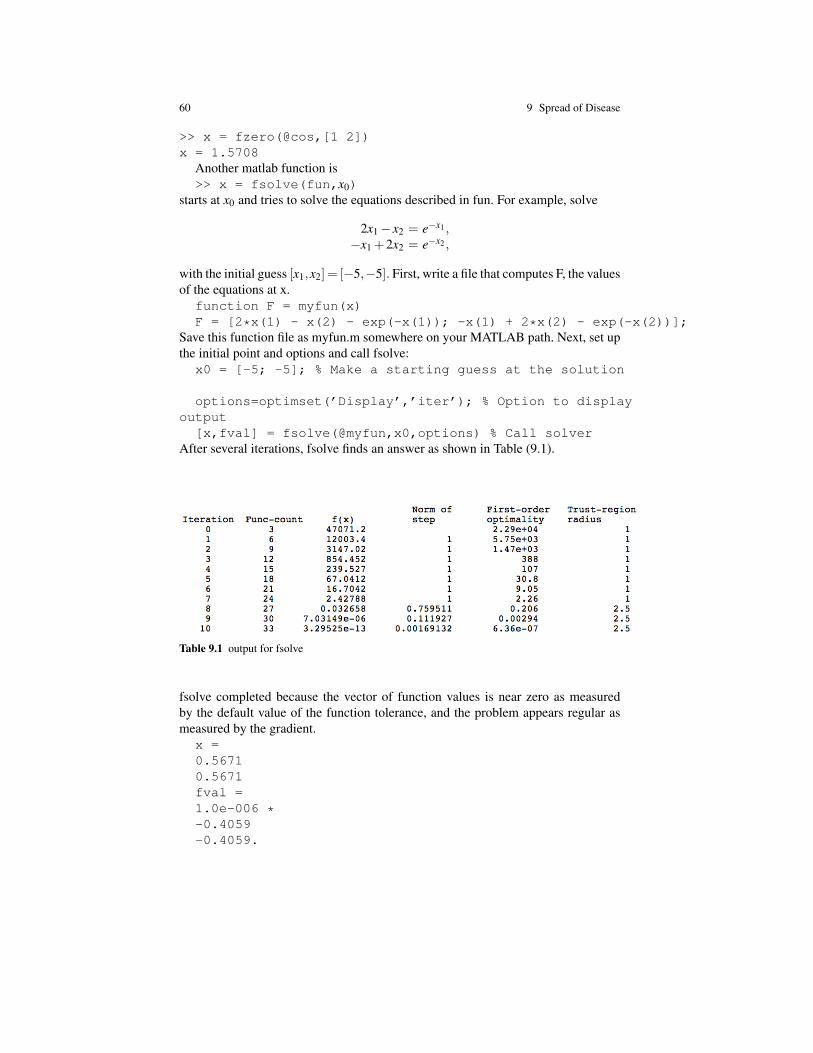
60 9 Spread of Disease
>> x = fzero(@cos,[1 2])x = 1.5708
Another matlab function is>> x = fsolve(fun,x0)
starts at x0 and tries to solve the equations described in fun. For example, solve
2x1− x2 = e−x1 ,−x1 +2x2 = e−x2 ,
with the initial guess [x1,x2] = [−5,−5]. First, write a file that computes F, the valuesof the equations at x.
function F = myfun(x)F = [2*x(1) - x(2) - exp(-x(1)); -x(1) + 2*x(2) - exp(-x(2))];
Save this function file as myfun.m somewhere on your MATLAB path. Next, set upthe initial point and options and call fsolve:
x0 = [-5; -5]; % Make a starting guess at the solution
options=optimset(’Display’,’iter’); % Option to displayoutput
[x,fval] = fsolve(@myfun,x0,options) % Call solverAfter several iterations, fsolve finds an answer as shown in Table (9.1).
Table 9.1 output for fsolve
fsolve completed because the vector of function values is near zero as measuredby the default value of the function tolerance, and the problem appears regular asmeasured by the gradient.
x =0.56710.5671fval =1.0e-006 *-0.4059-0.4059.
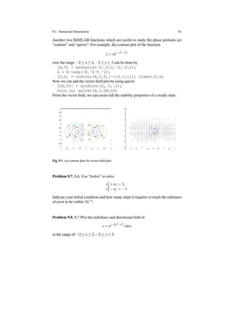
9.1 Numerical Simulations 61
Another two MATLAB functions which are useful to study the phase protraits are“contour” and “quiver”. For example, the contour plot of the function
z = xe(−x2−y2)
over the range −2≤ x≤ 2,−2≤ y≤ 3 can be done by[X,Y] = meshgrid(-2:.2:2,-2:.2:3);Z = X.*exp(-X.ˆ2-Y.ˆ2);[C,h] = contour(X,Y,Z,[-1:0.1:1]); clabel(C,h)
Now we can add the vector field plot by using quiver[DX,DY] = gradient(Z,.2,.2);hold on; quiver(X,Y,DX,DY)
From the vector field, we can easier tell the stability properties of a steady state.
Fig. 9.1 (a) contour plot (b) vector field plot
Problem 9.7. 8.6. Use “fsolve” to solve
x31 + x2 = 1,
x32− x1 = −1.
Indicate your initial condition and how many steps it requires to reach the toleranceof error to be within 10−6.
Problem 9.8. 8.7 Plot the nullclines and directional field of
z = e(−2x2−y2) sinx
in the range of −2≤ x≤ 2,−2≤ y≤ 3.


Chapter 10Enzyme Dynamics
Cells are the basic units of life. A cell consists of a concentrated aqueous solution ofmolecules contained in a membrane, called plasma membrane. A cell is capableof replicating itself by growing and dividing. Cells that have a nucleus are calledeukaryotes, and cells that do not have a nucleus are call prokaryotes. Bacteriaare prokaryotes, while yeast and amoebas, as well as most cells in our body, areeukaryotes. The Deoxyribonucleic acid (DNA) are very long polymeric molecules,consisting of two strands of chains, having double helix configuration, with repeatednucleotide units A, C, G, and T. The DNA is packed in chromosomes, within thenucleus in eukaryotes. In humans, the number of chromosomes is 46, except insperm and egg cells where the number is 23.
The DNA is the genetic code of the cell; it codes for proteins. Proteins lie mostlyin the cytoplasm of the cells, that is, outside the nucleus; some proteins are attachedto the plasma membrane, while some can be found in the nucleus. Proteins are poly-mers of amino acids whose number typically ranges from hundreds to thousands;there are 20 different amino acids from which all proteins are made. Each protein as-sumes 3-dimensional configuration, called conformation. Proteins perform specifictasks by changing their conformation.
Two proteins, A and B, may combine to form a new protein C. We express thisprocess by writing
A+B−→C.
Biological processes within a cell involves many such reactions. Some of these re-actions are very slow, other are very fast, and in some cases the reaction rate maystart slow, then speed up until it reaches a maximal level. In this chapter we considerthe question: How to determine the speed of biochemical reactions among proteins.In order to address this question we shall develop some mathematical models.
We begin with a simple case. Suppose we have two proteins, A and B, or moregenerally, two molecules A and B. We assume that A and B, when coming in contact,undergo a reaction, at some rate k1, that make them form a new molecule C. Weexpress this reaction by writing
63
64 10 Enzyme Dynamics
A+Bk1−→C;
k1 is called the rate coefficient. The respective concentrations of three moleculesare denoted by [A], [B], and [C]. The law of mass action states that the reaction rated[C]dt , or v1, of the above reaction is given by
v1 = k1[A][B],
that is,d[C]
dt= k1[A][B] (10.1)
Note that the above reaction implies that
d[A]at
=−k1[A][B],d[B]at
=−k1[A][B].
If the reaction is reversible with rate coefficient k−1, then
A+Bk1⇀↽k−1
C
andd[C]
dt= k1[A][B]− k−1[C],
d[A]dt
=d[B]dt
=−k1[A][B]+ k−1[C].
Metabolism in a cell is the sum of physical and chemical processes by whichmaterial substances are produced, maintained or destroyed, and by which energy ismade available. Enzymes are proteins that act as catalysts in speeding up chemicalreactions within a cell. They play critical roles in many metabolic processes withinthe cell. An enzyme, say E, can take a molecule S and convert it to a molecule P inone millionth of a second. The original molecule S is referred to as the substrate,and P is called the product. The enzyme-catalyzed conversion of a substrate S intoa product P is written in the form
S E−→ P. (10.2)
Figure 10.1 illustrate how an enzyme can convert substrate S into a product P.The profile [S]−→ [P] can take different forms, depending on the underlying biol-
ogy. Two typical profiles are shown in Figure 10.2.Figures 10.2(A) and 10.2(B) have been shown to hold in different experiments,
but it would be useful to derive them by mathematical analysis based on knownproperties of enzymes. Indeed such a derivation will give us a precise mathematicalformula for the profiles displayed in Figure 10.2. We begin with the derivation of aformula that yields the profile of Figure 10.2(A).

10 Enzyme Dynamics 65
S" S"P"
(a)" (b)" (c)" (d)" (e)"
Fig. 10.1 (a) Enzyme attracts S; (b) S is inside E; (c) Enzymatic process converts S into P; (d) Pis released; (e) Enzyme is ready to attract another S.
d[P
]/d
t
(A) [S]
d[P
]/d
t
(B) [S]
Fig. 10.2 Two different profiles of the enzymatic conversion of S−→ P.
In what follows we show how such a profile can be derived from the law of massaction. We write, schematically,
S+Ek1⇀↽k−1
C
where C is the complex SE,
Ck2−→ E +P.
By the law of mass action
d[C]
dt= k1[S][E]− (k−1 + k2)[C], (10.3)
d[E]dt
= −k1[S][E]+ (k−1 + k2)[C], (10.4)
d[S]dt
= −k1[S][E]+ k−1[C], (10.5)
d[P]dt
= k2[C]. (10.6)
66 10 Enzyme Dynamics
Notice thatddt([E]+ [C]) = 0
so that [E]+ [C] = const = e0; e0 is the total concentration of the enzyme in both Eand the complex C. Note that d[C]
dt + d[S]dt + d[P]
dt = 0, so equation (10.5) depends onequations (10.4) and (10.6) and may therefore be dropped.
We focus on equation (10.3) and note that in the enzymatic process the complexC changes very fast. Hence d[C]/dt is approximately zero, so that
k1[S][E]− (k−1 + k2)[C] = 0.
Substituting [E] = e0− [C] we get
k1[S](e0− [C]) = (k−1 + k2)[C]
or
[C] =k1e0[S]
(k−1 + k2)+ k1[S]=
e0[S]kM +[S]
where KM =k−1+k2
k1.
Thend[P]dt
= k2[C] = k2e0c =Vmax[S]KM +[S]
(10.7)
where Vmax = k2e0.we have thus derived the Michaelis-Menten formula
d[P]dt
=Vmax[S]KM +[S]
(10.8)
where Vmax and KM are constants; note that
d[P]dt→Vmax as [S]→ ∞.
The assumption we made in the derivation of (10.8) that d[C]/dt is very small isquite reasonable and, indeed, the Michaelis-Menten formula is widely used in de-scribing enzymatic processes.
But what about Figure 10.2(B)? Such a profile is based on a different enzymaticprocess, for example when an enzyme E can bound first with one substrate S andthen with another substrate S. Furthermore, in such a case, as is well establishedexperimentally, the speed by which the enzyme bounds with the second substrate ismuch faster, as illustrated in Figure 10.3.
We model such processes as follows:
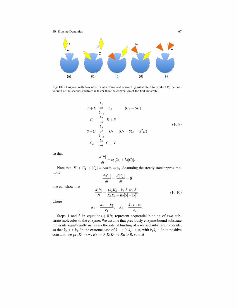
10 Enzyme Dynamics 67
S" P"
(a)" (b)" (c)" (d)" (e)"
S" P"
Fig. 10.3 Enzyme with two sites for absorbing and converting substrate S to product P; the con-version of the second substrate is faster than the conversion of the first substrate.
S+Ek1⇀↽k−1
C1, (C1 = SE)
C1k2→ E +P
S+C1
k3⇀↽k−3
C2 (C2 = SC1 = S2E)
C2k4→ C1 +P
(10.9)
so thatd[P]dt
= k2[C1]+ k4[C2].
Note that [E]+ [C1]+ [C2] = const.= e0. Assuming the steady state approxima-tions
d[C1]
dt=
d[C2]
dt= 0
one can show thatd[P]dt
=(k2K2 + k4[S])e0[S]K1K2 +K2[S]+ [S]2
, (10.10)
whereK1 =
k−1 + k2
k1, K2 =
k−3 + k4
k3.
Steps 1 and 3 in equations (10.9) represent sequential binding of two sub-strate molecules to the enzyme. We assume that previously enzyme-bound substratemolecule significantly increases the rate of binding of a second substrate molecule,so that k3 >> k1. In the extreme case of k1→ 0, k3→ ∞, with k1k3 a finite positiveconstant, we get K1→ ∞, K2→ 0, K1K2→ KH > 0, so that
68 10 Enzyme Dynamics
d[P]dt
=Vmax[S]2
KH +[S]2(10.11)
where Vmax and KH are constants. Formula (10.11) is called the Hill kinetics; itdisplays a profile similar to Figure 10.2(B).
Some enzymes can bound with three or more substrates. In this case it is oftenthe case that when enzyme has already bounded with m substrates S, it has a greateraffinity to bound with the next substrate S. Under this biological assumption, onecan derive the Hill kinetics of order n,
d[P]dt
=Vmax[S]n
KH +[S]n. (10.12)
The Michaelis-Menten formula is used also in other biological processes. For ex-ample, when macrophages M ingest bacteria B they become infected macrophagesMi. The resulting growth in Mi is described by the Michaelis-Menten formula
d[Mi]
dt= λ [M]
[B]K +[B]
.
Notice that for small [B], this is approximately the mass conservation law
M+B→Mi.
However the capacity of macrophages to ingest bacteria is limited by the followingfact: After receptor proteins on the macrophage membrane have been engaged in theingestion process, they need to take time off for recycling. Hence there is a limit, λ ,on how fast macrophages can ingest the bacteria.
Problem 10.1. Consider the chemical reactions
A+B k−→C, B+C k−→ A
with [A]+ [C] = 3 at time t = 0. Show that y = [B] satisfies y(t) = y0e−3kt .
Problem 10.2. The law of mass action can be extended to interaction among threeor more molecules. Consider for example three species X1,X2,X3 that interact toform a species Y :
X1 +X2 +X3k−→ Y
where k is the reaction rate. Then the law of mass action states that
d[Xi]
dt=−k[X1][X2][X3] for i=1,2,3.
In particular, if X1 = A, X2 = X3 = B, Y =C, then
A+2B k−→C
and

10.1 Numerical Simulations 69
d[A]dt
= −k[A][B]2,
d[B]dt
= −2k[A][B]2.
Assuming that 2[A(0)]+ [B(0)] = 1, show that y(t) = [B(t)] satisfies the equation
y′ =−ky2(1− y), 0 < y(t)< 1
if 0 < y(0)< 1, that the solution of the above equation is given by
1y+ ln
1− yy
= kt +C, C constant,
and that y(t)→ 0 as t→ ∞
Problem 10.3. Derive Equation (10.10) under the steady state approximations d[C1]/dt =0, d[C2]/dt = 0.
10.1 Numerical Simulations
Problem 10.4. SupposeA+B k−→C, C 3−→ A+B
Set x = [A], y = [B], z = [C] and take x(0) = y(0) = 1, z(0) = 8. Derive a systemof differential equations for x(t),y(t),z(t), and compute x(0) as a function of k, for1≤ k ≤ 5.
Problem 10.5.A+B k−→C, C 3−→ A+2B
Set x = [A], y = [B], z = [C] and take x(0) = y(0) = 1, z(0) = 8. Derive a systemof differential equations for x(t),y(t),z(t), and compute x(0) as a function of k, for1≤ k ≤ 5.

Chapter 11Bifurcation Theory
Consider two populations, x and y, that are interacting either by competition, or aspredator and prey. They may end up near a stable steady state, or possibly in sea-sonally varied states; this depends on their proliferation rates, death rates, availableresources, climate change, etc. In this chapter we wish to explore theses varied pos-sibilities using mathematics. To do that we begin by a short introduction the theoryof bifurcations. The change that occurs at p = pc typically involves two or morebranches of solutions which depend on the parameter p; the nature of these ‘bi-furcation’ branches changes radically at p = pc. Bifurcation theory is concernedwith the question of how the behavior of a system which depends on a parameterp changes with the parameter. It focuses on any critical value, p = pcr, where thebehavior of the system undergoes radical change; such values are called bifurca-tion points. We shall consider bifurcation phenomena for a system of differentialequations with parameter p,
dxdt
= f(x, p). (11.1)
Bifurcation points can arise in different ways. For example, suppose a steady stateof Equation (11.1), which depends on p, is stable for p < pc but loses stability at pc.Then a qualitative change has occurred in the phase portrait of the system (11.1), andp = pc is a bifurcation point. It sometimes happens that as p increases from p < pcto p > pc the differential system will begin to have periodic solutions, a well rec-ognized biological phenomena. Thus we would like to determine, mathematically,when such a situation takes place.
Problem 11.1-11.3 are simple but typical examples of bifurcations that frequentlyoccur in biology.
Problem 11.1. Consider the equation
dxdt
= p+ x2.
71

72 11 Bifurcation Theory
It has two steady states x = ±√−p if p < 0 and no steady states if p > 0. Prove
that x = −√−p is stable and x = +
√−p is unstable. The point p = 0 is called a
saddle-point bifurcation.
Problem 11.2. Consider the equation
dxdt
= px− x2.
It has steady points x = 0 and x = p. Prove that x = 0 is stable if p < 0 and unstableif p > 0, and x = p is unstable if p < 0 and stable if p > 0. Such a point p = 0,where there is an exchange of stability in the branches of the steady points, is calleda transcritical bifurcation.
Problem 11.3. Consider the equation
dxdt
= px− x3.
Show that x = 0 and x =±√p (for p > 0) are the steady states of this equation, anddetermine their stability. The point p = 0 is called a pitchfork bifurcation.
Figure 11 illustrates the last three examples.
(a)$ (b)$ (c)$
Fig. 11.1 (a) Saddle-point bifurcation diagram; (b) transcritical bifurcation diagram. (c) Pitchforkbifurcation. Solid curves represent stable steady states, while dotted curves are unstable steadystates.
Consider a species x with logistic growth whose death rate is a parameter p,
dxdt
= rx(1− xK)− px.
It has two steady states: x = 0 and x = K(1− pr ), but the last one is biologically
feasible only if x > 0, that is, if p < r. The two branches of steady points intersectat p = r where exchange of stability occurs: x = 0 is stable if p > r and unstable ifp< r, whereas x=K(1− p
r ) is stable if p< r and unstable if p> r. Thus transcriticalbifurcation occurs at p = r.

11 Bifurcation Theory 73
When the density of species x is very small (say 0 < x < 1) mating becomesdifficult: The probability of a male from x to meet and mate with a female from x isproportional to x2. Hence instead of growth rates
dxdt
= rx, ordxdt
= rx(1− xK)
we have growth rates
dxdt
= rx2, ordxdt
= rx2(1− xK).
Consider species x with dynamics
dxdt
= rx2(1− xK)− px.
It has three branches of steady points given by x = 0 and
rx(1− xK)− p = 0, or x =
K2±√
K2
4− p
r.
In this example pitchfork bifurcation occurs at p= r4 K2. We next consider a different
type of bifurcation whereby steady points bifurcate into periodic solutions; this ofcourse must involve a dynamical system with at least two equations.
Consider the following system of two equations, with bifurcation parameter p:
dx1
dt= px1−µx2−ax1(x2
1 + x22), (11.2)
dx2
dt= µx1 + px2−ax2(x2
1 + x22), (11.3)
where µ , a are positive constants. It is easily seen that the point x = 0 is a steadypoint, stable if p < 0 and unstable if p > 0. But for p > 0 there also exists a periodicsolution,
x1(t) =√
pa
cos µt, x2(t) =√
pa
sin µt
which traces the circle x21 + x2
2 =pa as t varies.
This type of bifurcation, which gives rise to periodic solutions, is called Hopfbifurcation. Note that the Jacobian matrix J at the (0,0), where the bifurcationoccurs, is given by
J =
(p −µ
µ p
),
and the characteristic equation is
(p−λ )2 +µ2 = 0,
74 11 Bifurcation Theory
so that the eigenvalues areλ = p± iµ.
As p crosses from p < 0 to p > 0, the two eigenvalues, at p = 0, become pureimaginary numbers. It is this behavior of the eigenvalues of the Jacobian matrix thatgives rise to the periodic solutions. In fact, the bifurcation behavior in the exampleof the system (11.2)-(11.3) is a special case of the following theorem.
Theorem 11.1. (Hopf Bifurcation) Consider the system
dxdt
= f (x,y, p),dydt
= g(x,y, p). (11.4)
Assume that for all p in some interval there exists a steady state (xs(p),ys(p)), andthat the two eigenvalues of the Jacobian matrix (evaluated at the steady state) arecomplex numbers λ1(p) = α(p)+ iβ (p) and λ2(p) = α(p)− iβ (p). Assume alsothat
α(p0) = 0, β (p0) 6= 0 anddα
d p(p0) 6= 0.
Then one of the three cases must occur:
1. there is an interval p0 < p < c1 such that for any p in this interval there existsa unique periodic orbit containing (xs(p0),ys(p0)) in its interior and having adiameter proportional to |p− p0|1/2;
2. there is an interval c2 < p < p0 such that for any p in this interval there exists aunique periodic orbit as in case (1);
3. for p = p0 there exist infinitely many orbits surrounding (xs(p0),ys(p0)) withdiameters decreasing to zero.
In the special case of (11.2)-(11.3), p0 = 0, (xs(p0),ys(p0)) = (0,0), α(p) = p,β (p) = µ , and both cases (1) and (3) occur; case (3) is illustrated in Fig. 3.1(F).
As first example of Hopf bifurcation we consider a model of herbivore-plantinteraction. The plant P has logistic growth with capacity K, and the herbivore Nhas eating capacity σ , which is the bifurcation parameter.
Problem 11.4. Consider a herbivore-plant model
dPdt
= rP(1− PK)−σ
P1+P
N,
dNdt
= γσP
1+PN−µN,
where γ is the yield constant and µ is the death rate of the herbivore. Prove that ifγ = 2µ , K = 10 then Hopf bifurcation occurs at σ = 5+
√25−11/2. [Hint: The
steady state for each σ is
P =µ
γσ −µ, N =
rσ(1+P)(1− P
K) =
rγ
γσ −µ(1− µ
K(γσ −µ)).
11 Bifurcation Theory 75
The Jacobian matrix is
J =
(P(− r
K + σN(1+P)2 ) −σ
P1+P
γσN(1+P)2 0
).
Write the eigenvalue equation in the form λ 2 + aλ + b = 0, and show that a = 0,b > 0, da
dσ< 0 at σ = 5+
√25−11/2. ]
Setting σ∗ = 5+√
25−11/2 we conclude that, as σ increases and crosses σ∗,the stable steady equilibrium (P,N) becomes unstable and instead the dynamicsof the herbivore-plant model develops periodic solutions with diameters which in-crease with σ . Thus both plant and herbivore will coexist, and their populations willvary “seasonally”.
Neuronal oscillations are periodic electrical oscillations along the axon of theneurons, and some simplified models represent them in the form
dvdt
= f (v)−w+ I,
dwdt
= ε(γv−w)
where I is the applied current, arriving from dendrites, which triggers the oscilla-tions. The function f (v) is a cubic polynomial and ε is a small parameter. The di-ameter of the periodic oscillations depends on f but is independent of the parameterI. Motivated by this model we consider here the case where f is a quadratic poly-nomial, and show that this case gives rise to Hopf bifurcation, that is, to periodicoscillations which begin with small diameter as I crosses a bifurcation parameterI0, and then increase with I proportionally to (I − I0)
1/2. For simplicity we takef (v) = v2.
Problem 11.5. Consider a system
dvdt
= v2−w+ I,
dwdt
= 2γv−w,
where γ > 14 and 0 < I < γ2. Show that the only steady state (v, w) is given by
v = γ −√
γ2− I, w = 2γ v, that it is stable if I < γ − 14 , and that Hopf bifurcation
occurs at I = γ− 14 .

76 11 Bifurcation Theory
11.1 Endangered Species
Species with very small density v is endangered as a result of endemic incurabledisease caused by a parasite with density w. If the population of v is spread over alarge territory then mating between a male from v and female from v is proportionalto v× v = v2. Hence
dvdt
= rv2−αvw
where α is the rate by which the parasite w depletes v. On the other hand, the growthof the parasite is proportional to v, so that
dwdt
= γv−βw
where β is the death rate of w. If rβ −αγ 6= 0 then the only steady point is (v, w) =(0,0). In order to save the endangered species v from extinction, new population ofthe species are introduced into the territory, at density rate I, so that
dvdt
= rv2−αvw+ I.
This results in steady point (v, w) where v > 0, w > 0, and the question arises: arethese points (v(I), w(I)) stable for all I?
To address this question we take, for simplicity, r = α = β = 1, and 1 < γ < 2.Then
dvdt
= v2−wv+ I,
dwdt
= γv−w.
The only steady point is w = γ v, v = ( Iγ−1 )
1/2, and the Jacobian matrix about (v, w)is
I =((2− γ)v −v
γ −1
).
Hence detJ = 2(γ−1)> 0 and
trace J = (2− γ)(I
γ−1)1/2−1≡ A(I)
where A(I)< 0 if I < I0, A(I)> 0 if I > I0, and
I0 =γ−1
(2− γ)2 .
The eigenvalues of J areλ = σ ± iτ
11.2 Numerical Simulations 77
where σ = 12 A(I), τ = [( 1
2 A(I))2−2(γ−1)]1/2, and dσ
dI > 0 at I = I0. Hence (v, w)is a stable steady point if I < I0, and Hopf bifurcation occurs at I = I0. We concludethat as I is increased the population v, in the steady state, will increase and remainstable as long as I < I0; thereafter the steady point will become unstable, and thepopulations of v and w will oscillate periodically.
Problem 11.6. Consider the following predator-prey model with sparse prey popu-lation, x,
dxdt
= x2(1− x)− xy
dydt
= 4xy−4αy
where α > 0. It has an equilibrium point (α,α(1−α)) for any 0 < α < 1. Provethat Hopf bifurcation occurs at α = 1
2 .
The biological interpretation is that if the predator death rate is smaller than 2then both predator and prey coexist in steady state, but if the predator death rate ex-ceeds 2 then both predator and prey still coexist but their densities vary periodically,or “seasonally”.
11.2 Numerical Simulations
To plot the bifurcation diagram, one needs to scan through the parameter spaceand solve the ODEs for those parameters. If we would like to plot the bifurcationdiagram for
dxdt
= f (x, p),
the first step is to plot the the nullcline on the x-p plane ( f (x, p) = 0), which cor-reponds to the steady states xs under different p. On the nullcline, part of the curvecorresponds to stable steady state, and part of that corresponds to unstable steadystate (of course, it is possible that only one of them exist). Let us consider the ex-ample
dxdt
= x2 + p.
First we would like to plot the curve of x2+ p = 0 on x-p plane. In MATLAB, definethe right-hand-side function in a script file:
function y = saddlefun(p,x)y = p + x.ˆ2;Note that p and x could be matrices (so is y) in order to accomodate the dis-
cretized mesh grid matrix of x-p space. To plot the bifurcation diagram, we createbifur.m, a function file (see Algorithm 1)., with inputs the name of the function (e.g.’saddlefun’) and the range of x and p to plot. In bifru.m, we first discretize x-p plane

78 11 Bifurcation Theory
in 101 by 101 mesh grid (use the command ’meshgird’). Then we try to fplot thezeros of x2 + p by using the ’contour command, as shown in Fig. Next, for each p,we need to start with an initial condition x0 which is NOT a steady state and seeat what steady state it ends up. To achieve that, we avoid the nullclines (by using| f (xi, p j)|> 0.1×mean| f (xi, p j)|), use the rest of the points as intial conditions andsolve the ODE. The solution will get away from the unstable steady state (branch)and be attracted to stable steady state (branch) (Fig.).
p
x
−5 −4 −3 −2 −1 0 1 2 3 4 5−5
−4
−3
−2
−1
0
1
2
3
4
5
p
x
−5 −4 −3 −2 −1 0 1 2 3 4 5−5
−4
−3
−2
−1
0
1
2
3
4
5
p
x
−5 −4 −3 −2 −1 0 1 2 3 4 5−5
−4
−3
−2
−1
0
1
2
3
4
5
Fig. 11.2 Bifurcation diagram for saddle point bifurcation. (a) Red curves are the steady states;(b) green circles are non-steady-state points; (c) solutions converge to stable steady states (bluecircles).
Problem 11.7. Plot the bifrcation diagram for
dxdt
= px− x3.
with range −5≤ p≤ 5,−5≤ x≤ 5.

11.2 Numerical Simulations 79
Algorithm 3 bifur.m% BIFUR Draws bifurcation diagrams% BIFUR(FCN,XRANGE,PRANGE) draws the% bifurcation diagram % for the function FCN over the specified x and p ranges.% FCN is a handle to a user-defined function that takes as% arguments a variable x and a parameter p. XRANGE is a% row vector of the form [XMIN XMAX]. PRANGE is a row vector % of the form [PMINPMAX].%% Example:% bifur(@saddlefun,[-5 5],[-5 5]);%% where saddlefun is a user-defined function of the form%% function y=saddlefun(x,p)% y=p+x.ˆ2;%function bifur(fcn,xrange,prange)nn = 100; % number of points plotted in each rangep1 = [prange(1):(prange(2)-prange(1))/nn:prange(2)]; % sample points in px1 = [xrange(1):(xrange(2)-xrange(1))/nn:xrange(2)]; % sample points in x[p,x] = meshgrid(p1,x1); % generate grid points in [p,x]fval = feval(fcn,x,p); % evaluate the points valuefigure(1);[c,h] = contour(p,x,fval,[0,0],’r’); % plot the zero contour linexlabel(’p’), ylabel(’x’) x = x(:); p = p(:);ind = find(abs(fval)¿0.05*mean(abs(fval(:))));x = x(ind); p = p(ind);if 1figure(1); hold on; plot(p,x,’go’) % draw the initial pointsendfor iter = 1:1000x = x + 0.05*feval(fcn,x,p); % solve odeend hold on; plot(p(:),x(:),’bo’)

Chapter 12Atherosclerosis: the risk of high cholesterol
Arteries are blood vessels that carry oxygen-rich blood to the heart, brain and otherparts of the body. Atherosclerosis is a disease in which a plaque builds up insidearteries. The plaque consists of cholesterol, calcium, cells from the blood, and cellsfrom the arterial wall. Over time the plaque grows, hardens, and narrows the artery.This reduces the flow of oxygen-rich blood, and also make it more likely to causea blood clot, or thrombus, that will block the blood flow. A blockage formed in thecoronary arteries may trigger a heart attack. A blockage formed in the carotid artery(located on each side of the neck, feeding oxygen to the brain) may cause a stroke.Atheroselerosis is the leading cause of death in the United States and worldwide,with annual deaths of 900,000 in the United States and 13 millions worldwide.
The exact cause of atheroselerosis is unknown, and in many cases there are nosymptoms until an episode of heart attack or stroke occurs. There are however riskfactors which contribute to the disease, namely, high cholesterol, heavy smoking,and hypertension. In this chapter we focus on the risk associated with high choles-terol, and use mathematics to quantify this risk.
Cholesterol is a protein that each cell in our body needs, But cholesterol does notdissolve in blood, and must therefore be transported in the blood stream. It is trans-ported by carrier called lipoprotein, made of fat (lipid) and protein. There are twotypes of lipoproteins that carry the cholesterol to and from cells. They are called:low-density lipoproteins, LDL, and high-density lipoproteins, HDL. The LDL are“bad” cholesterols, and the HDL are “good” cholesterols. The LDL contributesto plaque growth and the HDL reduce the plaque by removing the LDL from theplaque.
The level of cholesterol in the blood is measured in units of 10−5gm/cm3. TheAmerican Heart Association established guidelines regarding the atherosclerosisrisk associated with the levels of LDL and HDL in the blood. For example,
LDL=190, HDL=40 is high risk,LDL=110, HDL=50 is risk free.In this chapter, we develop a mathematical model of plaque growth and use it to
predict the risk associated with any pair of values (LDL, HDL). We introduce thenotation
81

82 12 Atherosclerosis: the risk of high cholesterol
L0 = Concentration of LDL in blood,H0 = Concentration of HDL in blood,
and wish to determine, based on (L0,H0), whether a plaque will grow or shrink. Todo that we need to understand how a plaque is formed.
Under the pressure of the bloodstream, a small lesion may occur in the inner sur-face of the arterial wall, enabling cholesterol to invade into the inner layer, calledintima. Free radicals are molecules or ions that have umpaired valence electrons,and are therefore highly reactive in many chemical processes in our body; they playuseful role in metabolic processes. Macrophages are cells of the immune systemthat travel around the body and engulf and digest foreign particles, cellular debris,and invading microorganisms. When LDL enters the intima, they immediately be-come oxidized by radicals. Macrophages from the blood then move into the intimaand engulf the oxidized LDL. The fat-laden macrophages saturated with oxidizedLDL, are called foam cells. Figure 12.1 shows a cross section of a plaque in theartery.
Blood%
Artery%wall%
Macrophage%
Foam%cell%
Cholesterol%%molecules%
Fig. 12.1 Cross section of a plaque in an artery.
In our mathematical model we assume that the plaque consists mainly of macrophagesand foam cells. This is a simplification, since also other cells are involved, such assmooth muscle cells which move from the middle layer of the arterial wall into theintima.
Our model will include the following variables:
• Macrophage density, M,• Foam cell density, F ,• “Bad” cholesterol concentration, LDL or L,• “Good” cholesterol concentration, HDL or H.
We shall not distinguish between LDL and oxidized LDL. The equation for LDL isthe following:
dLdt
= L0− k1ML
K1 +L− r1L. (12.1)

12 Atherosclerosis: the risk of high cholesterol 83
The first term on the right-hand side, L0, is the LDL concentration in the blood. Thesecond term represents the ingestion of LDL by macrophages, which is describedby the Michaelis-Menten formula. The last term is the degradation of LDL.
In a similar way we write the equation for HDL:
dHdt
= H0− k2HF
K2 +F− r2H. (12.2)
Here the second term on the right-hand side is interpreted as follows: HDL is be-ing absorbed by a foam cell (more precisely, it forms a complex with a membraneprotein of a foam cell) and this initiates a process that empties out the oxidizedLDL from the foam cell. The foam cells returns to become a macrophage, while theemptied-out oxidized LDL is removed from the plaque and is transported back (bythe blood) to the liver for recycling. We note that when H forms a complex with areceptor protein on F , it takes some time for the receptor to again become free. Thusthe receptor “recycling” limits the ability of F to react to H, and this explains whywe used k2HF/(K2 +F) instead of k2HF in Eq. (12.2).
The equations for macrophages and foam cells are
dMdt
=−k1ML
K1 +L+ k2H
FK2 +F
+λML
δ +H−µ1M, (12.3)
dFdt
= k1ML
K1 +L− k2H
FK2 +F
−µ2F. (12.4)
The first two terms or the right-hand sides of Eqs. (12.3)-(12.4), account for theexchanges between macrophages and foam cells, as already explained above. Theterms µ1M, µ2F represent the natural deaths of macrophages and foam cells. Theremaining term that needs explanation is λML/(δ +H). The oxidized LDL in theplaque triggers infiltration of macrophages from the blood into the plaque, and this isaccounted by the factor λML. On the other hand, the HDL are oxidized by radicals(as the LDL are) and this reduces the amount of radicals available to oxidize LDL.In this sense H acts as inhibitor, which restricts the effect of λML by a factor 1/(δ +H), for some δ > 0.
We wish to solve the system of equations (12.1)-(12.4) and compute the weightof the plaque
w(t) = M(t)+F(t)
at time t; the weight of the cholesterol is negligible. We take initial values
L = 0,H = 0,F = 0,M = M0 = 5×10⁻⁴g/cm3.
We set
R(t) =w(t)w(0)
=w(t)M0
so that R(0) = 1.
84 12 Atherosclerosis: the risk of high cholesterol
Given cholesterol level (L0,H0), we wish to determine whether R(t) will in-crease, indicating risk of atherosclerosis, or decrease which means risk-free ofatherosclerosis.
The following problems show that if L0 is sufficiently small then R(t)→ 0 ast → ∞, that is: if the level of “bad” cholesterol is low then there is no risk of aplaque to form.
Problem 12.1. Show that for any small ε > 0, L(t)< L0r1+ε if t is sufficiently large.
Problem 12.2. Assume that µ1 = µ2 = µ and prove that if
L0 <r1δ µ
λ
then R(t)→ 0 if t→ ∞.
12.1 Numerical Simulations
We wish to compute R(t) for 0 < t < T , say T = 300 days.We say that (L0,H0) is in the risk zone if R(T )> 1, and in the risk-free zone if
R(T )< 1. In the following simulations we use the parameters taken from the modeldeveloped in []: k1 = 144/day, k2 = 10/day, K1 = 10−2g/cm3, K2 = 0.5 g/cm3,µ1 = 0.015/day, µ2 = 0.03/day, r1 = 2.4× 10⁻⁵/day, r2 = 5.5× 10⁻⁷/day, λ =2.57×10⁻³/day, δ =−2.54 g/cm3.
Problem 12.3. Compute R(300) (300 days) for the 25 pairs (L0,H0), where L0 =100,120,140,160,180 and H0 = 40,45,50,55,60.
Problem 12.4. Verify that in each of these cases R(300) > 1 if L0 > µ1λ(δ +H0),
and R(300)< 1 if L0 <µ1λ(δ +H0).
We may thus conclude that, roughly, (L0,H0) is in the risk zone if
L0 >µ1
λ(δ +H0),
and in the no-risk zone ifL0 <
µ1
λ(δ +H0).
The borderline between the two zones is the linear L0 = aH +b where a = µ1λ,b =
µ1λ
δ .
Chapter 13Cancer-immune Interaction
An abnormally new growth of tissue with cells that grow more rapidly than normalcells and has no physiological function is called a neoplasm or a tumor. The ab-normally rapidly growing cells compete with normal cells for space and nutrients.When the new growth is localized, it is called a benign tumor. When a tumor in tis-sue has reaches a size of several millimeters it requires a large supply of nutrients,for otherwise it can no longer grow. Such a tumor is called avascular. Avasculartumors try to induce the formation of new blood vessels (angiogenesis) and directtheir movement toward them. They do so by secreting tumor endothelial growthfactor (VEGF) and, if successful, the tumors become vascular. A vascular tumorcontinues to grow and some of its cells may break away and travel to other parts ofthe body through the bloodstream or the lymph system. Metastatic cancer is a tu-mor that spread from the original location where it started to other parts of the body.Metastatic cancer is also called malignant cancer, or, briefly, cancer, although peo-ple often use the words tumor and cancer interchangeably. Most cancer deaths aredue to metastasized cancer.
Cancer is a disease of tissue growth failure, and it is the result of normal cellstransforming into cancer cells because of mutations in genes that regulate cellgrowth and differentiation. In the context of cancer, these genes are classified eitheras oncogenes or tumor suppressor genes. Oncogenes are genes which promotecell growth and reproduction. Tumor suppressor genes are genes which inhibit celldivision and survival. Malignant transformation occurs when oncogenes becomeoverexpressed compared to normal oncogenes, or when tumor suppressor genes be-come underexpressed, or disabled. Typically a transformation of a normal cell to atumor cell occurs after not one but several gene mutations.
It is commonly believed that most mutations leading to cancer are due to externalconditions, such as smoking, dietary factors, environmental pollutants, exposure toradiation, and certain infections. But some mutations are hereditary.
There are more than one hundred known types of human cancer, broadly catego-rized according to the tissue of origin. Carcinomas begin with epithelial cells; sar-comas arise from connective tissues, muscles and vasculature; leukemias and lym-phomas are cancers of the hematopoietic (blood) and immune system, respectively;
85
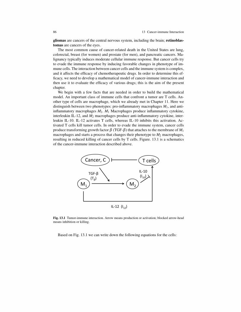
86 13 Cancer-immune Interaction
gliomas are cancers of the central nervous system, including the brain; retinoblas-tomas are cancers of the eyes.
The most common cause of cancer-related death in the United States are lung,colorectal, breast (for women) and prostate (for men), and pancreatic cancers. Ma-lignancy typically induces moderate cellular immune response. But cancer cells tryto evade the immune response by inducing favorable changes in phenotype of im-mune cells. The interaction between cancer cells and the immune system is complex,and it affects the efficacy of chemotherapeutic drugs. In order to determine this ef-ficacy, we need to develop a mathematical model of cancer-immune interaction andthen use it to evaluate the efficacy of various drugs; this is the aim of the presentchapter.
We begin with a few facts that are needed in order to build the mathematicalmodel. An important class of immune cells that confront a tumor are T cells. An-other type of cells are macrophage, which we already met in Chapter 11. Here wedistinguish between two phenotypes: pro-inflammatory macrophages M1, and anti-inflammatory macrophages M2. M1 Macrophages produce inflammatory cytokine,interleukin IL-12, and M2 macrophages produce anti-inflammatory cytokine, inter-leukin IL-10. IL-12 activates T cells, whereas IL-10 inhibits this activation. Ac-tivated T cells kill tumor cells. In order to evade the immune system, cancer cellsproduce transforming growth factor β (TGF-β ) that attaches to the membrane of M1macrophages and starts a process that changes their phenotype to M2 macrophages,resulting in reduced killing of cancer cells by T cells. Figure. 13.1 is a schematicsof the cancer-immune interaction described above.
Cancer,(C( T(cells(
M1( M2(
TGF1β((Tβ)((
IL110((I10)(
IL112(((I12)(
Fig. 13.1 Tumor-immune interaction. Arrow means production or activation; blocked arrow-headmeans inhibition or killing.
Based on Fig. 13.1 we can write down the following equations for the cells:

13 Cancer-immune Interaction 87
dCdt
= λcC(1− CC0
)−µcTC, (13.1)
dM1
dt= k1− γM1
Tβ
k1 +Tβ
−µM1, (13.2)
dM2
dt= γM1
Tβ
k1 +Tβ
−µM2, (13.3)
dTdt
= kTI12
k2 + I10−µT T. (13.4)
We also have the following equations for the cytokines:
dI12
dt= λ12M1−µ12I12, (13.5)
dI10
dt= λ10M2−µ10I10, (13.6)
dTβ
dt= λβC−µβ Iβ . (13.7)
In Eq. (13.1) we assume a logistic growth for cancer cells, and that T cells killcancer cells at rate µc. In Eq. (13.2) we assume constant production rate k1 anddeath rate µ1 of M1 macrophage. Tβ changes the phenotype of M1 to M2, and this is
accounted by the term γM1Tβ
k1+Tβ
. In Eq. (13.4) the first term represents the activation
of T cells by I12, a process inhibited by I10 which appears in the factor 1/(k2 + I10).We simplify the model (13.1)-(13.6) by noting that the cytokines dynamics is
much faster than the cells dynamics. Hence we may assume steady state in the equa-tions of (13.5)-(13.7). Thus I12 = const M1, I10 = const M2 and Tβ = const C. Usingthese relations in Eqs. (13.2)-(13.4), the system (13.1)-(13.7) reduces to the follow-ing system of four equations:
dCdt
= λcC(1− CC0
)−µcTC, (13.8)
dM1
dt= k1− γM1
CK1 +C
−µM1, (13.9)
dM2
dt= γM1
CK1 +C
−µM2, (13.10)
dTdt
= kTM1
K2 +M2−µT T. (13.11)
with coefficients γ , kT and K1,K2.A common chemotherapeutic drug is TGF-β inhibitor. The effect of this drug is
to increase µβ and hence to reduce γ .
Problem 13.1. Use Eq. (13.5) to deduce that for any small ε > 0,
88 13 Cancer-immune Interaction
M1(t)≤k1
µ+ ε
if t is large enough.
Problem 13.2. Use Eq. (13.9) to deduce that for any small ε > 0,
M1(t)≥k1
µ + γ− ε
if t is large enough.
Problem 13.3. Use Eq. (13.10) to deduce that for any small ε > 0,
M2(t)≤γk1
µ2 + ε
if t is large enough.
Problem 13.4. Use Eq. (13.11) to deduce that for any small ε > 0,
T (t)≥ kT
α(γ)− ε
if t is large enough, where
α(γ) =µT
k1(µ + γ)(k2 + γk1/µ
2).
Problem 13.5. Use Eq. (13.8) and Problem 13.4 to conclude that if
kT µC > λcα(γ). (13.12)
then limt→∞ C(t) = 0.
The coefficients kT and µC depend on the immune system, i.e., on the responseof the T cells to cancer. The aggressiveness of the cancer depends on TGF-β , thatis, on the parameter γ , which may be decreased by TGF-β inhibitor. Problem 13.5asserts that is the immune system is strong enough relative to the aggresiveness ofthe cancer then the cancer will disappear.
13.1 Numerical Simulations
We would like to investigate how effective the drug is for various “strengths” µc ofthe T-cells killing rate. So we shall determine how C(t), say for 0 ≤ t ≤ 60 days,depends on the drug and on the immune strength (µc). All other parameters are givenas follows: kc = 10−2/day, µc = 10−7/cell/day, C0 = 106 cell/cm3, µ = 0.3/day,

13.1 Numerical Simulations 89
k1 = 3000 cell/cm3/day, γ = 1.1µ /day, kT = 2µT /cell/day, K1 = 0.5C0, K2 =105 cell/cm3, µT = 0.2/day.
Problem 13.6. Solve the model (13.6)-(13.11) under the initial conditions C(0) =102 cell/cm3, M1(0) = 5× 10⁴ cells/cm3, M2(0) = 0, T (0) = 0, for 0 ≤ t ≤ 60days.
Problem 13.7. Repeat the calculation with γ replaces by γ/A, A = 2,5,10 and drawthe 3 profiles of C(t), 0≤ t ≤ 60.
Problem 13.8. Repeat Problem 11.2 with
1. µc replaced by µc10 .
2. µc replaced by 10µc.
Draw conclusions on how the efficacy of TGF-β inhibitor on the strength of theimmune system parameter µc.

Chapter 14Cancer Therapy
There are many drugs that are used in the treatment of cancer; some drug kill cancercells directly while others change the cancer microenviroment to make it resistant tocancer cells growth. In Chapter 11, we considered the drug TGF-β inhibitor, whichchanges the macrophage phenotype, thereby enabling the immune system to killcancer cells more effectively.
In this chapter we consider two entirely different kinds of anti-cancer drugs. Thefirst one blocks the activity of VEGF, and the second one uses virus to kill tumorcells.
14.0.1 VEGF receptor inhibitor
In order to continue to grow abnormally, the tumor requires increasing amounts ofoxygen from the blood. So the tumor secrets VEGF which attracts endothelial cellsthat from the inner lining of the blood vessels wall, thereby leading to the formationof new blood vessels (angiogenesis) that deliver oxygen to the tumor. To model thisprocess we introduce the following variables:
c = density of tumor cells,e = density of endothelial cells,h = concentration of VEGF,w = concentration of oxygen,
We assume logistic growthλ1c(1− c
K)
of the tumor, where K is the carrying capacity and λ1 is the growth rate. We assumethat λ1 is proportional to w, λ1 = 0 if w = 0, and that
w = Be (B a positive constant). (14.1)
91
92 14 Cancer Therapy
Hence,dcdt
= λ1ec(1− cK)−µ1c, c(0)< K. (14.2)
Here λ1 is a positive constant and µ1 is the death rate of cancer cells.Next we model the equation for VEGF by
dhdt
= λ2c−µ2h, (14.3)
where λ2 is the production rate of VEGF by tumor cells, and µ2 is the degradationrate.
Endothelial cells proliferation is assumed to be proportional to h,
dedt
= λ3h.
But we need to take into account that e is proportional to w (by Eq. (14.1)) whereasoxygen is decreased by consumption by cancer cells as well by dissipation in thetissue, that is,
dwdt
=−µ3cw− µ4w.
Hence the complete equation for e has the form
dedt
= λ3h−µ3ce−µ4e, (14.4)
where all the parameters are positive constants.Avastin is a drug that inhibits VEGF receptor (VEGFR) and thus does not allow
the activation of VEGF. We can model the effect of Avastin by replacing λ2 in Eq.(14.3) by λ2/(1+A) where A is proportional to the amount of the delivered drug.Then Eq. (14.3) becomes
dhdt
=λ2c
1+A−µ2h. (14.5)
The following problems show that if A is large enough then the tumor will decreaseto zero as t→ ∞.
Problem 14.1. Observe that c(t)< K for all t > 0, and use Eq. (14.5) to show that,for any ε > 0,
h(t)≤ λ2Kµ2(1+A)
+ ε if t is large enough.
Problem 14.2. Use Eq. (14.4) and Problem 14.1 to show that, for any ε > 0,
e(t)≤ λ2λ3Kµ2µ4(1+A)
+ ε if t is large enough.
Problem 14.3. Use Eq. (14.2) and Problem 14.2 to show that if
14 Cancer Therapy 93
1+A >λ1λ2λ3Kµ1µ2µ4
then c(t)→ 0 as t→ ∞.
We concluded that if Avastin is administered in large enough amount then thetumor will shrink to zero. We note however that Avastin has negative side effects,including damage to the liver, and thus can only be administered in limited amounts.
We next introduce a completely different model for anti-tumor treatment byblocking VEGF. We begin with a model of cancer cells suggested by Gumpertz.It includes cancer cells x and growth factor γ which act, like VEGF, to provide nu-trients to the cancer:
dxdt = γx,dγ
dt = −αγ.(14.6)
Problem 14.4. Prove that the solution of (14.6) satisfies the Gompertz equation
dxdt
=−αx lnxK, (0 < x < K) (14.7)
where K is given by
lnx(0)
K=−γ(0)
α.
We view K as the carrying capacity and α as the growth rate. The constant K de-pends on the density of the blood vessels which provides nutrients to the tumor. Wecan refine the model (14.7) by taking K to be a function of the concentration of theblood capillaries, which we shall denote by y. We take K = y so that
dxdt
= αx lnxy, (14.8)
and model the concentration y by the equation
dydt
= A−2µy+δxy. (14.9)
Here A−2µy represents that natural growth and degradation of capillaries, and δxyrepresents the formation of new capillaries from existing capillaries, induced bygrowth factors secreted by the tumor cells.
Problem 14.5. The system (14.8)-(14.9) has steady states
x = y = Z± where Z± =1δ{µ±
√µ2−δA},
provided δA < µ2. Prove that the steady state x = y = Z− is stable, and that thesteady state x = y = Z+ is unstable.
The biological interpretation is that (i) if δA > µ2, then the tumor receives suffi-cient nutrients so it grows indefinitely (no steady states); (ii) if δA < µ2, there willbe a steady state (benign tumor).

94 14 Cancer Therapy
We recall that tumor secrets VEGF that increase angiogenesis, and hence A. Adrug that blocks VEGF such as soluble VEGFR-1 (e.g. Avastin), reduces A. If thedrug decreases A so that δA < µ2, then the tumor will not grow indefinitely. Fur-thermore, the drug will also decrease the size of the benign tumor, in the sense thatit decreases the stable steady point with x = y = 1
δ(µ−
√µ2−δA).
14.0.2 Virotherapy
We next consider anti-cancer drug which employs virus particles to kill cancer cells;such a treatment is called virotherapy. The virus particles are genetically modifiedso that they can infect cancer cells but not normal healthy cells. Such viruses arecalled oncolytic viruses. The viruses are injected directly into the tumor.
After entering a cancer cell, a virus begins to quickly replicate, and when thecancer cell dies, a large number of virus particles burst out and proceed to infectother cancer cells.
To model this process we introduce the following variables:
x = number density of cancer cells,y = number density of infected cancer cells,n = number density of dead cells,v = number density of virus particles which are not contained in cancer cells,
Virotherapy is modeled by the following system of equations:
dxdt = λx−βxv,dydt = βxv−δy,dndt = δy−µn,dvdt = bδy− γv.
(14.10)
where
λ = proliferation rate of cancer cells,β = rate of infection of cancer cells by viruses,δ = death rate of infected cancer cells,µ = removal rate of debris of dead cells,
and, finally, b is the replication number of a virus at the time of death of the infectedcancer cell. Adding Eqs. (14.10), we get
ddt(x+ y+n) = λx−µn. (14.11)

14.1 Numerical Simulations 95
We assume that the tumor is spherical with radius R(t) and that the cells arecontinuously moving around in a way that keeps their distribution constant withinthe sphere. Hence
x(t)+ y(t)+n(t) = θ(t) (14.12)
where θ(t) is the total cell density. By (14.11), the increase in the number of cellsin the growing sphere is given by
ddt(
4π
3R3(t)θ(t)) = (λx(t)−µn(t))
4π
3R3(t).
We assume that θ(t) is approximately a constant θ0. Then, after using also(14.12) we get
θ03R
dRdt
= (λ +µ)x+µy−µθ0 (14.13)
where x and y satisfy the first two equations of (14.10) and v satisfies the last equa-tion of (14.10).
In experiments, viral therapy as described above was not initially successful be-cause it failed to address the effect of the immune system. Immune cells recognizethe infected cancer cells and destroy them before the virus particles get a chanceto replicate to their full potential. To make virotherapy more effective the immunesystem must therefore be suppressed. In Problem 14.8 we extend the model (14.10)-(14.13) to include the density of the immune cells, z, and the chemotherapy P whichsuppresses the immune system.
Problem 14.6. Show that the system for (x,y,v) in (14.10) has a steady point (x, y, v)with x > 0, and determine whether it is asymptotically stable.
14.1 Numerical Simulations
To simulate the model (14.10)-(14.13), we provide the following codes which uses’ode45’ to solve the ODEs.
Problem 14.7. Take λ = 2×10⁻²/h, δ =(1/18)/h, µ =(1/48)/h, θ0 = 106 cells/mm3,β = 7×10⁻⁸ mm3/(h·virus), γ = 2.5×10⁻²/h. Compute R(t) for 0≤ t ≤ 20h, withinitial conditions x0 = 8×10⁵ cells/mm3, y0 = 105 cells/mm3, v0 = 109 virus/mm3,R(0) = 2 mm when b = 50,100,200,500.
Problem 14.8. Consider the system
dxdt
= λx−βxv,dydt
= βxv− kyz−δy,
dndt
= kyz+δy−µn,dzdt
= syz−ωz2−P(t)z,dvdt
= bδy− k0vz− γv,

96 14 Cancer Therapy
Algorithm 4 model cancer.m% This code simulates model (14.10)-(14.13).close all,clear all,% define global parametersglobal lambda delta mu theta 0 beta gamma b% starting and final timet0 = 0; tfinal = 20;% paramterslambda = 2 * 10ˆ-2; delta = 1/18; mu = 1/48; theta 0 = 10ˆ6; beta = 7 * 10ˆ-8; gamma = 2.5 *10ˆ-2;b = 100;% initial conditionsv0 = [8*10ˆ5, 10ˆ5, theta 0-8*10ˆ5-10ˆ5, 10ˆ9, 2];[t,v] = ode45(’fun cancer’,[t0,tfinal],v0);plot(t,v(:,5)) % Plot the evolution of the radius of tumor
Algorithm 5 fun cancer.m% This is the function file called by model cancer.mfunction dy = fun cancer(t,v)global lambda delta mu theta 0 beta gamma bdy(1) = lambda*v(1) - beta*v(1)*v(4);dy(2) = beta*v(1)*v(4) - delta*v(2);dy(3) = delta*v(2) - mu*v(3);dy(4) = b*delta*v(2) - gamma*v(4);dy(5) = v(5)/(3*theta 0)*((lambda+mu)*v(1)+mu*v(2)-mu*theta 0);dy = [dy(1);dy(2);dy(3);dy(4);dy(5)];
where z = number density of immunity cells, P(t) = immune suppressor drug, x+y+n+z = θ0, k = rate of immune cell killing infected cell, k0 = take-up rate of virusby immune cells, s = stimulation rate of immune cells by infected cells, ω = clearingrate of immune cells. We take P(t)= 8×10⁻²/h, k = 2×10⁻⁸ mm3/(h·immune cell),k0 = 10−8 mm3/(h·immune cell), s = 5.6×10⁻⁷ mm3/(h·infected cell), ω =2×10⁻⁷
mm3/(h·immune cell) and all other parameters as in Problem 14.7, z0 = 6× 10⁴
cells/mm3, and all other initial conditions as in Problem 14.7. (i) Compute R(t)for 0 ≤ t ≤ 20h, when b = 50,100,200,500 and compare the results with those ofProblem 14.7. (ii) Do the same when the chemotherapy dose is increased to P(t) =16×10−2/h.

Chapter 15Turberculosis
Tuberculosis (TB) is an infective disease caused by Mycobacterium tuberculosis(Mtb). The bacteria is spread through the air when people who have active TB in-fection cough or sneeze. The bacteria attack the lungs, primarily, but can also spreadand attack other parts of the body. The most common symptom of active TB infec-tion is chronic cough with blood-tinged sputum. It is estimated that one-third of theworld’s population have been infected with Mtb, although only 13 million chroniccases were active globally in 2013, and 1.5 million associated death occurred. Treat-ment of TB uses antibiotics to kill the bacteria, but the treatment is not entirelyeffective. Vaccination, in children decreases significantly the risk of infection.
TB infection in the lungs begins when inhaled mycrobacteria tuberculosis reachthe pulmonary alveoli and invade into, or are ingested by, alveoli macrophages; alve-oli are tiny air sacs within the lungs where exchange of oxygen and carbon dioxidetakes place. It is clearly important to determine whether infection by inhaled Mtbwill develop into chronic TB. This cannot be determined directly by measurement,so we shall use mathematics to address this question. In what follows we developa mathematical model and use it to determine the threshold of initial infection thatwill develop into active TB.
We introduce the following variables:
M = number of alveolar macrophages in cm3;Mi = number of infected alveolar macrophages in cm3;Be = number of extracellular bacteria (residing in tissue, outside macrophages) in cm3;Bi = number of intracellular bacteria (residing inside macrophages) in cm3;
M satisfies the differential equation
dMdt
= µM−λ1MBe
K +Be−dMM. (15.1)
Here µM is the production rate of M and dM is the death rate when there is not infec-tion; in steady state, µM = dMM0 where M0 is the number of macrophages in cm3 in
97
98 15 Turberculosis
healthy lungs. The second term on the right-hand side of Eq. (15.1) represents theingestion of bacteria by macrophages, modeled by the Michaelis-Menten formula,which turns M into Mi.
The infected macrophages satisfy the equation
dMi
dt= λ1M
Be
K +Be−λ2Mi
B2i
B2i +(NMi)2 −dMiMi. (15.2)
The first term on the right-hand side comes from macrophages ingesting extracellu-lar bacteria, and dMi is the death rate of Mi macrophages. The second term on theright-hand side of Eq. (15.2) accounts for the burst of Mi under bacterial load. Theprobability for macrophage burst increase to 50% when the number of internal bac-teria reaches N, that is, when Bi = NMi, the burst rate is λ2/2. Note that we haveassumed here that the transition from non-bursting state to bursting-state is sharp,as in Fig. 10.2(B) rather than Fig. 10.2(A), and so we used the Hill kinetics ratherthan the Michaelis-Menten law.
We next write a differential equation for the extracellular bacteria:
dBe
dt= Nλ2Mi
B2i
B2i +(NMi)2 −λ1M
Be
K +Be. (15.3)
The first term on the right-hand side accounts for the number of bacteria released atburst of infected macrophages, and the second term represents the loss of Be due toingestion by macrophages.
The equation for intracellular bacteria Bi is
dBi
dt= γBi +λ1M
Bc
K +Bc−Nλ2Mi
B2i
B2i +(NMi)2 . (15.4)
The bacteria grow within macrophages at rate γ . The last two terms in Eq. (15.4)have already been explained above.
The question then arises: How does it happen that most infections with Mtb donot lead to chronic active TB? The answer is that the adaptive immune system (lo-cated in the lymph nodes) receives stress signals from the Mi, and then inflammatorymacrophages (in contrast to non-inflammatory alveolar macrophages) and T cellsmigrate into the lung and kill bacteria. For simplicity we consider only the T cells.Their number per cm3, satisfies the equation
dTdt
= αMi−dT T, (15.5)
where dT , and α is the rate by which T cells are activated by the (signaling sent bythe) Mi. The killing of bacteria means that we have to replace Eqs. (15.3)-(15.4) bythe following equations:

15 Turberculosis 99
dBe
dt= Nλ2Mi
B2i
B2i +(NMi)2 −λ1M
Be
K +Be−δ1T Be, (15.6)
dBi
dt= γBi +λ1M
Be
K +Be−Nλ2Mi
B2i
B2i +(NMi)2 −δ2T Bi, (15.7)
For simplicity we take δ1 = δ2 = δ . The parameters α,δ determine the course ofthe Mtb infection.
The question of susceptibility to TB can be framed as follows: how many in-gested bacteria it takes to cause an initial infection to develop into chronic TB? Weshall address this question with the following simple model which involves onlyextracellular bacteria B and uninfected macrophages M:
dMdt
= M0−µ1MB
B+K−αM, (15.8)
dBdt
= λB−µ2MB
B+K. (15.9)
Here M0 is a baseline supply of new macrophages, α is the natural death rate ofmacrophages, µ1 is the rate by which macrophages ingest bacteria, a process thatdepletes the bacteria at rate µ2, and λ is the ingestion process (or endocytosis) mod-eled by the Michaelis-Menten law because the uptake of bacteria by a macrophageis time-limited. In steady state of healthy individuals M0−αM = 0.
The model (15.8)-(15.9) is very simple since, as we know from the more de-tailed model (15.1)-(15.7), λ is a function of Bi, Mi and T . Nevertheless, already thepresent simple model sheds some light on the consideration of susceptibility to TB,as we see from the following problems.
Problem 15.1. We may view the system (15.8)-(15.9) as a model of an infectionsdisease with DFE
(M,B) = (M0
α,0).
Setting
b =µ2M0
α−λK,
show that the DFE is stable if b > 0 and unstable if b < 0.
We next study the behavior of solutions of Eqs. (15.8)-(15.9) when the initialvalues are not necessarily near the DFE.
Problem 15.2. Show that if M(0) ≤ M0α
then M(t) ≤ M0α
for all t > 0, and deducethat
dBdt≥ B
λB−bB+K
.
Problem 15.3. Deduce from Problem 15.2 that if initially M0 ≤ M0α
and B(0)> b/λ
then B(t)→ ∞ as t → ∞, which means that TB will develop; note that if b < 0 weonly need to assume that M(0)≤ M0
αand B(0)> 0.
100 15 Turberculosis
We next show that if M(0) > M0α
and b > 0 then small infection with Mycobac-teria tuberculosis does not result in TB. Let ε be so small that if
β = α +µ1ε
ε +K
thenM(0)>
M0
Band (since b > 0) λ <
µ2M0
β (ε +K). (15.10)
We shall prove that if B(0)< ε the B(t)< ε for all t > 0. Indeed, otherwise there isa first time t0 such that
B(t)< ε if t < t0, and B(t0) = ε.
It follow thatdBdt
(t0)≥ 0 (15.11)
andB(t)
B(t)+K<
ε
ε +Kif t < t0.
Hence, by (15.8),
dMdt
> M0−µ1Mε
ε +K−αM = M0−βM. (15.12)
Rewriting (15.12) in the form
ddt(Meβ t)> M0eβ t
we obtain, by integration,
M(t)> M(0)e−β t +M0
β− M0
βe−β t >
M0
βfor 0 < t ≤ t0
where we used the inequality M(0) > M0β
from (15.10). We now use Eq. (15.9) todeduce that
dBdt
(t0) = (λ − µ2MB+K
)B|t=t0 < (λ − µ2MB+K
)ε < 0
by the second inequality in (15.10), and this is a contradiction to (15.11).
Problem 15.4. Use the last result and Problem 15.2 to show that if M(0) > M0α
,b > 0 and B(0) is sufficiently small then (M(t),B(t))→ (M0
α,0) as t → ∞. [Hint:
show that that M(t)− M0α
<Cε if t is large, where C is a constant.]

15.1 Numerical Simulations 101
15.1 Numerical Simulations
In the following problems the parameters of the system (15.1)-(15.4) are given asfollows: λ1 = 14/day, λ2 = 0.05/day, dM = 8×10⁻³/day, M0 = 1.5×10⁶ cell/cm3,so that µM = dMM0 = 1.2× 10⁴ cell/day, dMi = 5× 10⁻²/day, K = 105Be/cm3,γ = 0.8 day. At the beginning of infection with Mtb we have: M =M0,Mi = 0,Bi = 0and Be is the number of inhaled bacteria per cm3. We also take dT = 0.3/day,α = 2.5/day and T (0) = 0.
Problem 15.5. Simulate the model (15.1)-(15.5) for 0< t < 30 days with Be(0) = 1.You should find that the functions Be(t),Bi(t) are monotonically increasing.
Problem 15.6. Take δ = 0.1 and Be(0) = 2,5,10. In each of these three cases, com-pute Be(30) and Bi(30).
Problem 15.7. Repeat the calculations of Problem 15.6 with δ = 1 and with δ = 5.


![Mathematical Models in Biology - Bio · PDF fileMathematical Models in Biology ... J.D., Mathematical Biology, Springer, 1989, [19] Edelstein-Keshet, Leah, Mathematical models in biology,](https://static.documents.pub/doc/80x56/5ab3fe3b7f8b9a7c5b8b587a/mathematical-models-in-biology-bio-models-in-biology-jd-mathematical-biology.jpg)