54
Introduction to Mathematical Fluid Dynamics-II Balance of Momentum Meng Xu Department of Mathematics University of Wyoming Bergische Universität Wuppertal Math Fluid Dynamics-II

Introduction to Mathematical Fluid Dynamics-IIBalance of Momentum
Meng Xu
Department of MathematicsUniversity of Wyoming
Bergische Universität Wuppertal Math Fluid Dynamics-II

Fluid path
Consider the path followed by a fluid particle flows inside adomain W .
x(t) = (x(t), y(t), z(t))
Then the velocity field becomes
u(x(t), y(t), z(t), t) = (x(t), y(t), z(t))
oru(x(t), t) =
dxdt
(t)
Bergische Universität Wuppertal Math Fluid Dynamics-II

Fluid path
Consider the path followed by a fluid particle flows inside adomain W .
x(t) = (x(t), y(t), z(t))
Then the velocity field becomes
u(x(t), y(t), z(t), t) = (x(t), y(t), z(t))
oru(x(t), t) =
dxdt
(t)
Bergische Universität Wuppertal Math Fluid Dynamics-II

Fluid path
Consider the path followed by a fluid particle flows inside adomain W .
x(t) = (x(t), y(t), z(t))
Then the velocity field becomes
u(x(t), y(t), z(t), t) = (x(t), y(t), z(t))
oru(x(t), t) =
dxdt
(t)
Bergische Universität Wuppertal Math Fluid Dynamics-II

Acceleration of fluid particle
Another physical quantity in fluid mechanics is the accelerationof the fluid particle
a(t) =d2
dt2 x(t) =ddt
u(x(t), y(t), z(t))
=∂u∂xx+
∂u∂yy +
∂u∂zz +
∂u∂t
Denote ux = ∂u∂x ,.. ut =
∂u∂t and
u(x, y, z, t) = (u(x, y, z, t), v(x, y, z, t),w(x, y, z, t))
Bergische Universität Wuppertal Math Fluid Dynamics-II

Material derivative
From the above notation, we can rewrite
a(t) = uux + vuy + wuz + ut
= ∂tu + u · ∇u
We will frequently use the operator
DDt
= ∂t + u · ∇ (1)
Operator (1) is called the material derivative.
Bergische Universität Wuppertal Math Fluid Dynamics-II

Material derivative
From the above notation, we can rewrite
a(t) = uux + vuy + wuz + ut
= ∂tu + u · ∇u
We will frequently use the operator
DDt
= ∂t + u · ∇ (1)
Operator (1) is called the material derivative.
Bergische Universität Wuppertal Math Fluid Dynamics-II
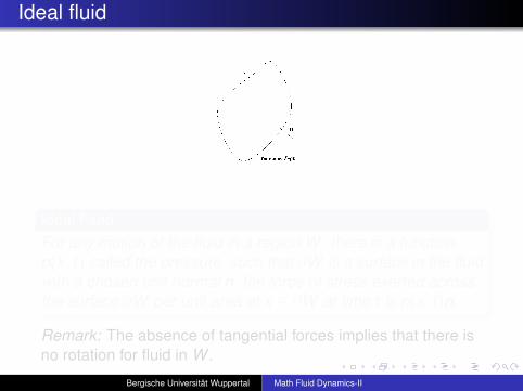
Ideal fluid
Ideal FluidFor any motion of the fluid in a region W, there is a functionp(x , t) called the pressure, such that ∂W is a surface in the fluidwith a chosen unit normal n, the force of stress exerted acrossthe surface ∂W per unit area at x ∈ ∂W at time t is p(x , t)n.
Remark: The absence of tangential forces implies that there isno rotation for fluid in W .
Bergische Universität Wuppertal Math Fluid Dynamics-II

Force on the boundary
For ideal fluid, the total force on the fluid inside W by means ofstress on its boundary is
S∂W = {force on W} = −∫∂W
pndA
For any fixed vector e, divergence theorem gives us
e · S∂W = −∫∂W
pe · ndA
= −∫
Wdiv(pe)dV
= −∫
W(gradp) · edV
HenceS∂W = −
∫W
gradpdV
Bergische Universität Wuppertal Math Fluid Dynamics-II

Balance of momentum
Denote b(x , t) as the given body force per unit mass, then thetotal body force is
B =
∫WρbdV
In all, force per unit volume is equal to
−gradp + ρb
Balance of Momentum(Differential Form)By the principle of momentum balance (Newton’s second law),
ρDuDt
= −gradp + ρb
Bergische Universität Wuppertal Math Fluid Dynamics-II

Integral form
An integral form of the balance of momentum can be derivedfor general fluid:
Balance of Momentum(Integral Form)
By the principle of momentum balance,
ddt
∫Wt
ρudV = S∂Wt +
∫Wt
ρbdV
Here Wt is a region at time t and S∂Wt represents the total forceexerted on the surface ∂Wt .
Bergische Universität Wuppertal Math Fluid Dynamics-II

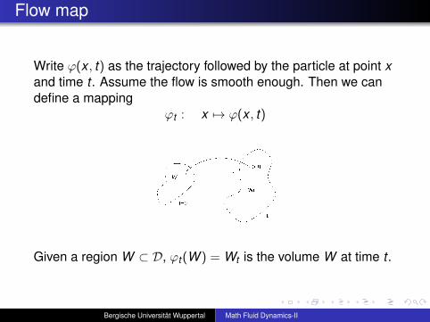
Flow map
Write ϕ(x , t) as the trajectory followed by the particle at point xand time t . Assume the flow is smooth enough. Then we candefine a mapping
ϕt : x 7→ ϕ(x , t)
Given a region W ⊂ D, ϕt(W ) = Wt is the volume W at time t .
Bergische Universität Wuppertal Math Fluid Dynamics-II
Flow map
Write ϕ(x , t) as the trajectory followed by the particle at point xand time t . Assume the flow is smooth enough. Then we candefine a mapping
ϕt : x 7→ ϕ(x , t)
Given a region W ⊂ D, ϕt(W ) = Wt is the volume W at time t .
Bergische Universität Wuppertal Math Fluid Dynamics-II

First lemma
The first lemma before we continue is the following
Lemma 1Define J(x , t) as the Jacobian determinant of the map ϕt , wehave
∂
∂tJ(x , t) = J(x , t) [divu(ϕ(x , t), t)]
We give a sketch of proof for this lemma.
Write the components of ϕ as ξ(x , t),η(x , t) and ζ(x , t). Then itsJacobian determinant can be written as
J(x , t) =
∂ξ∂x
∂η∂x
∂ζ∂x
∂ξ∂y
∂η∂y
∂ζ∂y
∂ξ∂z
∂η∂z
∂ζ∂z
Bergische Universität Wuppertal Math Fluid Dynamics-II

Proof of lemma 1
For fixed x ,
∂
∂tJ =
∂
∂t
∂ξ∂x
∂η∂x
∂ζ∂x
∂ξ∂y
∂η∂y
∂ζ∂y
∂ξ∂z
∂η∂z
∂ζ∂z
=
∂∂t∂ξ∂x
∂η∂x
∂ζ∂x
∂∂t∂ξ∂y
∂η∂y
∂ζ∂y
∂∂t∂ξ∂z
∂η∂z
∂ζ∂z
+
∂ξ∂x
∂∂t∂η∂x
∂ζ∂x
∂ξ∂y
∂∂t∂η∂y
∂ζ∂y
∂ξ∂z
∂∂t∂η∂z
∂ζ∂z
+
∂ξ∂x
∂η∂x
∂∂t∂ζ∂x
∂ξ∂y
∂η∂y
∂∂t∂ζ∂y
∂ξ∂z
∂η∂z
∂∂t∂ζ∂z
Bergische Universität Wuppertal Math Fluid Dynamics-II
By definition of the velocity field
∂
∂tϕ(x , t) = u(ϕ(x , t), t)
Thus∂
∂t∂ξ
∂x=
∂
∂x
∂ξ
∂t=
∂
∂xu(ϕ(x , t), t)
∂
∂t∂ξ
∂y=
∂
∂y
∂ξ
∂t=
∂
∂yu(ϕ(x , t), t)
.................................
∂
∂t∂ζ
∂z=
∂
∂z
∂ζ
∂t=
∂
∂zw(ϕ(x , t), t)
Bergische Universität Wuppertal Math Fluid Dynamics-II
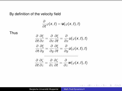
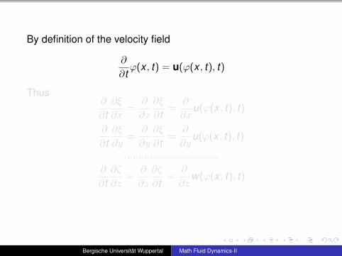
By definition of the velocity field
∂
∂tϕ(x , t) = u(ϕ(x , t), t)
Thus∂
∂t∂ξ
∂x=
∂
∂x
∂ξ
∂t=
∂
∂xu(ϕ(x , t), t)
∂
∂t∂ξ
∂y=
∂
∂y
∂ξ
∂t=
∂
∂yu(ϕ(x , t), t)
.................................
∂
∂t∂ζ
∂z=
∂
∂z
∂ζ
∂t=
∂
∂zw(ϕ(x , t), t)
Bergische Universität Wuppertal Math Fluid Dynamics-II
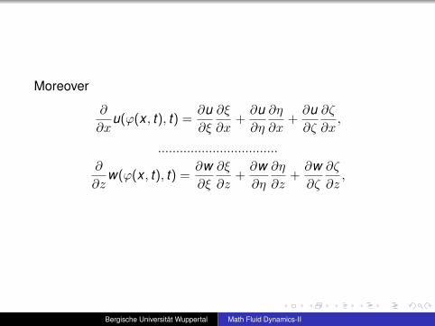
Moreover
∂
∂xu(ϕ(x , t), t) =
∂u∂ξ
∂ξ
∂x+∂u∂η
∂η
∂x+∂u∂ζ
∂ζ
∂x,
.................................
∂
∂zw(ϕ(x , t), t) =
∂w∂ξ
∂ξ
∂z+∂w∂η
∂η
∂z+∂w∂ζ
∂ζ
∂z,
Bergische Universität Wuppertal Math Fluid Dynamics-II
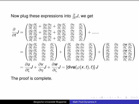
Now plug these expressions into ∂∂t J, we get
∂
∂tJ =
∂u∂ξ
∂ξ∂x + ∂u
∂η∂η∂x + ∂u
∂ζ∂ζ∂x
∂η∂x
∂ζ∂x
∂u∂ξ
∂ξ∂y +
∂u∂η
∂η∂y +
∂u∂ζ
∂ζ∂y
∂η∂y
∂ζ∂y
∂u∂ξ
∂ξ∂z +
∂u∂η
∂η∂z +
∂u∂ζ
∂ζ∂z
∂η∂z
∂ζ∂z
+ ......
=
∂u∂ξ
∂ξ∂x
∂η∂x
∂ζ∂x
∂u∂ξ
∂ξ∂y
∂η∂y
∂ζ∂y
∂u∂ξ
∂ξ∂z
∂η∂z
∂ζ∂z
+
∂ξ∂x
∂v∂η
∂η∂x
∂ζ∂x
∂ξ∂y
∂v∂η
∂η∂y
∂ζ∂y
∂ξ∂z
∂v∂η
∂η∂z
∂ζ∂z
+
∂ξ∂x
∂η∂x
∂w∂ζ
∂ζ∂x
∂ξ∂y
∂η∂y
∂w∂ζ
∂ζ∂y
∂ξ∂z
∂η∂z
∂w∂ζ
∂ζ∂z
=∂u∂ξ
J +∂v∂η
J +∂w∂ζ
J = [divu(ϕ(x , t), t)] J
The proof is complete.
Bergische Universität Wuppertal Math Fluid Dynamics-II

Second lemma
Lemma 2Given a scalar or vector function f (x , t), we have
ddt
∫Wt
f (x , t)dV =
∫Wt
[∂f∂t
+ div(fu)]
dV (2)
A similar result can be proved and is called the transporttheorem.
Transport Theorem
ddt
∫Wt
ρudV =
∫Wt
ρDuDt
dV (3)
Bergische Universität Wuppertal Math Fluid Dynamics-II

Second lemma
Lemma 2Given a scalar or vector function f (x , t), we have
ddt
∫Wt
f (x , t)dV =
∫Wt
[∂f∂t
+ div(fu)]
dV (2)
A similar result can be proved and is called the transporttheorem.
Transport Theorem
ddt
∫Wt
ρudV =
∫Wt
ρDuDt
dV (3)
Bergische Universität Wuppertal Math Fluid Dynamics-II

Second lemma
Lemma 2Given a scalar or vector function f (x , t), we have
ddt
∫Wt
f (x , t)dV =
∫Wt
[∂f∂t
+ div(fu)]
dV (2)
A similar result can be proved and is called the transporttheorem.
Transport Theorem
ddt
∫Wt
ρudV =
∫Wt
ρDuDt
dV (3)
Bergische Universität Wuppertal Math Fluid Dynamics-II

Proof of Lemma 2
Let us prove (2) first.
By change of variables formula and the first lemma
LHS =ddt
∫W
f (ϕ(x , t), t)J(x , t)dV
=
∫W
[dfdt
(ϕ(x , t), t)J + f (ϕ(x , t), t)∂J∂t
]dV
=
∫W
[DfDt
(ϕ(x , t), t) + divuf]
JdV
Bergische Universität Wuppertal Math Fluid Dynamics-II

Proof of Lemma 2
Let us prove (2) first.
By change of variables formula and the first lemma
LHS =ddt
∫W
f (ϕ(x , t), t)J(x , t)dV
=
∫W
[dfdt
(ϕ(x , t), t)J + f (ϕ(x , t), t)∂J∂t
]dV
=
∫W
[DfDt
(ϕ(x , t), t) + divuf]
JdV
Bergische Universität Wuppertal Math Fluid Dynamics-II

=
∫Wt
[DfDt
+ divuf]
dV
=
∫Wt
[∂f∂t
+ uf + divuf]
dV
=
∫Wt
[∂f∂t
+ div(fu)]
dV
Thus (2) is proved.
Bergische Universität Wuppertal Math Fluid Dynamics-II

To prove (3), we first observe that
ddt
(ρu)(ϕ(x , t), t) =DDt
(ρu)(ϕ(x , t), t)
This is because the time derivative takes into account the factthat the fluid is moving and that the positions of fluid particleschange with time. So, if f (x, y, z, t) is any function of positionand time, then by the chain rule
ddt
f (x(t), y(t), z(t), t)
= ∂t f + u · ∇f
=DfDt
(x(t), y(t), z(t), t)
Bergische Universität Wuppertal Math Fluid Dynamics-II

Using Lemma 1, we have
ddt
∫Wt
ρudV =ddt
∫W(ρu)JdV =
∫W
ddt
[(ρu)J]dV
=
∫W
DDt
(ρu)(ϕ(x , t), t)J + (ρu)(ϕ(x , t), t)∂
∂tJ(x , t)dV
=
∫W
[DDt
(ρu) + (ρdivu)u]
JdV
By the conservation of mass
DρDt
+ ρdivu =∂ρ
∂t+ div(ρu) = 0
Bergische Universität Wuppertal Math Fluid Dynamics-II

Using Lemma 1, we have
ddt
∫Wt
ρudV =ddt
∫W(ρu)JdV =
∫W
ddt
[(ρu)J]dV
=
∫W
DDt
(ρu)(ϕ(x , t), t)J + (ρu)(ϕ(x , t), t)∂
∂tJ(x , t)dV
=
∫W
[DDt
(ρu) + (ρdivu)u]
JdV
By the conservation of mass
DρDt
+ ρdivu =∂ρ
∂t+ div(ρu) = 0
Bergische Universität Wuppertal Math Fluid Dynamics-II

Thusddt
∫Wt
ρudV =
∫Wt
ρDuDt
dV
Bergische Universität Wuppertal Math Fluid Dynamics-II

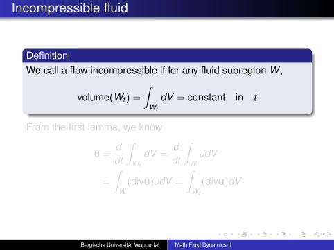
Incompressible fluid
DefinitionWe call a flow incompressible if for any fluid subregion W ,
volume(Wt) =
∫Wt
dV = constant in t
From the first lemma, we know
0 =ddt
∫Wt
dV =ddt
∫W
JdV
=
∫W(divu)JdV =
∫Wt
(divu)dV
Bergische Universität Wuppertal Math Fluid Dynamics-II
Incompressible fluid
DefinitionWe call a flow incompressible if for any fluid subregion W ,
volume(Wt) =
∫Wt
dV = constant in t
From the first lemma, we know
0 =ddt
∫Wt
dV =ddt
∫W
JdV
=
∫W(divu)JdV =
∫Wt
(divu)dV
Bergische Universität Wuppertal Math Fluid Dynamics-II

Incompressible fluid
DefinitionWe call a flow incompressible if for any fluid subregion W ,
volume(Wt) =
∫Wt
dV = constant in t
From the first lemma, we know
0 =ddt
∫Wt
dV =ddt
∫W
JdV
=
∫W(divu)JdV =
∫Wt
(divu)dV
Bergische Universität Wuppertal Math Fluid Dynamics-II
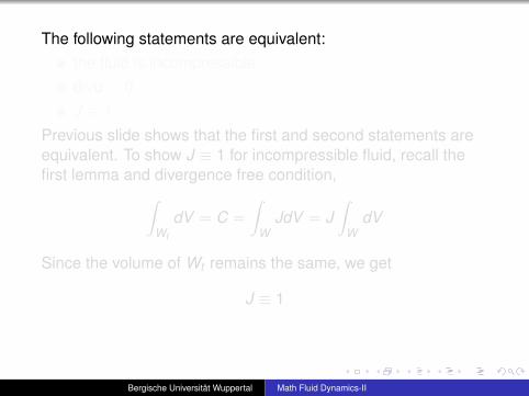
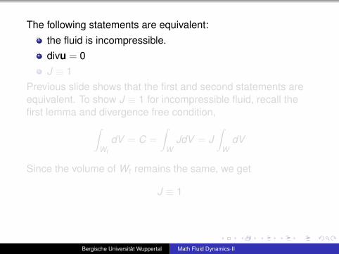
The following statements are equivalent:the fluid is incompressible.divu = 0J ≡ 1
Previous slide shows that the first and second statements areequivalent. To show J ≡ 1 for incompressible fluid, recall thefirst lemma and divergence free condition,∫
Wt
dV = C =
∫W
JdV = J∫
WdV
Since the volume of Wt remains the same, we get
J ≡ 1
Bergische Universität Wuppertal Math Fluid Dynamics-II

Continuity equation for incompressible fluid
Recall the continuity equation
DρDt
+ ρdivu = 0
For incompressible fluid, it reduces to
DρDt
= 0
Bergische Universität Wuppertal Math Fluid Dynamics-II

Continuity equation for incompressible fluid
Recall the continuity equation
DρDt
+ ρdivu = 0
For incompressible fluid, it reduces to
DρDt
= 0
Bergische Universität Wuppertal Math Fluid Dynamics-II


