55
Introduction to Mathematical Programming OR/MA 504 Chapter 5 Integer Linear Programming
| Date post: | 24-Dec-2015 |
| Category: |
Documents |
| Upload: | kathlyn-hood |
| View: | 239 times |
| Download: | 2 times |

Introduction toMathematical Programming
OR/MA 504
Chapter 5
Integer Linear Programming

6-2
Introduction• When one or more variables in an LP
problem must assume an integer value we have an Integer Linear Programming (ILP) problem.
• ILPs occur frequently…– Scheduling workers– Manufacturing airplanes
• Integer variables also allow us to build more accurate models for a number of common business problems.

6-3
Integrality ConditionsMAX: 350X1 + 300X2 } profit
S.T.: 1X1 + 1X2 <= 200 } pumps
9X1 + 6X2 <= 1566 } labor
12X1 + 16X2 <= 2880 } tubing
X1, X2>= 0 } nonnegativity
X1, X2 must be integers } integrality
Integrality conditions are easy to state but make the problem much more difficult (and sometimes impossible) to solve.

6-4
Relaxation• Original ILP
MAX: 2X1 + 3X2
S.T.: X1 + 3X2 <= 8.25
2.5X1 + X2 <= 8.75
X1, X2 >= 0
X1, X2 must be integers
• LP RelaxationMAX: 2X1 + 3X2
S.T.: X1 + 3X2 <= 8.25
2.5X1 + X2 <= 8.75
X1, X2 >= 0

6-5
Integer Feasible vs. LP Feasible Region
X1
X2
Integer Feasible Solutions
00
1 2 3 4
1
2
3

6-6
Solving ILP Problems• When solving an LP relaxation, sometimes
you “get lucky” and obtain an integer feasible solution.
• This was the case in the original Blue Ridge Hot Tubs problem in earlier chapters.
• But what if we reduce the amount of labor available to 1520 hours and the amount of tubing to 2650 feet?
See file Fig5-1.xls

6-7
Bounds
• The optimal solution to an LP relaxation of an ILP problem gives us a bound on the optimal objective function value.
• For maximization problems, the optimal relaxed objective function values is an upper bound on the optimal integer value.
• For minimization problems, the optimal relaxed objective function values is a lower bound on the optimal integer value.

6-8
Rounding• It is tempting to simply round a
fractional solution to the closest integer solution.
• In general, this does not work reliably:– The rounded solution may be infeasible.– The rounded solution may be suboptimal.

6-9
How Rounding Down Can Result in an Infeasible Solution
X1
X2
00
1 2 3 4
1
2
3
optimal relaxed solution
infeasible solution obtained by rounding down

6-10
Branch-and-Bound
• The Branch-and-Bound (B&B) algorithm can be used to solve ILP problems.
• Requires the solution of a series of LP
problems termed “candidate problems”.• Theoretically, this can solve any ILP.• Practically, it often takes LOTS of
computational effort (and time).

6-11
Stopping Rules• Because B&B can take so long, most ILP packages
allow you to specify a suboptimality tolerance factor.
• This allows you to stop once an integer solution is found that is within some % of the global optimal solution.
• Bounds obtained from LP relaxations are helpful here.– Example
• LP relaxation has an optimal obj. value of $64,306.• 95% of $64,306 is $61,090.• Thus, an integer solution with obj. value of $61,090
or better must be within 5% of the optimal solution.

6-12
Using Solver
Let’s see how to specify integrality conditions and suboptimality tolerances using Solver…
See file Fig5-2.xls

6-13
An Employee Scheduling Problem:Air-Express
Day of Week Workers NeededSunday 18
Monday 27
Tuesday 22
Wednesday 26
Thursday 25
Friday 21
Saturday 19
Shift Days Off Wage1 Sun & Mon $680
2 Mon & Tue $705
3 Tue & Wed $705
4 Wed & Thr $705
5 Thr & Fri $705
6 Fri & Sat $680
7 Sat & Sun $655

6-14
Defining the Decision Variables
X1 = the number of workers assigned to
shift 1
X2 = the number of workers assigned to
shift 2
X3 = the number of workers assigned to
shift 3
X4 = the number of workers assigned to
shift 4
X5 = the number of workers assigned to
shift 5
X6 = the number of workers assigned to
shift 6
X7 = the number of workers assigned to
shift 7

6-15
Defining the Objective Function
Minimize the total wage expense.MIN: 680X1 +705X2 +705X3 +705X4 +705X5 +680X6 +655X7

6-16
Defining the Constraints• Workers required each day
0X1+ 1X2+ 1X3+ 1X4+ 1X5+ 1X6+ 0X7 >= 18 } Sunday
0X1+ 0X2+ 1X3+ 1X4+ 1X5+ 1X6+ 1X7 >= 27 } Monday
1X1+ 0X2+ 0X3+ 1X4+ 1X5+ 1X6+ 1X7 >= 22 }Tuesday
1X1+ 1X2+ 0X3+ 0X4+ 1X5+ 1X6+ 1X7 >= 26 } Wednesday
1X1+ 1X2+ 1X3+ 0X4+ 0X5+ 1X6+ 1X7 >= 25 } Thursday
1X1+ 1X2+ 1X3+ 1X4+ 0X5+ 0X6+ 1X7 >= 21 } Friday
1X1+ 1X2+ 1X3+ 1X4+ 1X5+ 0X6+ 0X7 >= 19 } Saturday
• Nonnegativity & integrality conditionsXi >= 0 and integer for all i

6-17
Implementing the Model
See file Fig5-3.xls

6-18
Binary Variables
• Binary variables are integer variables that can assume only two values: 0 or 1.
• These variables can be useful in a number of practical modeling situations….

6-19
A Capital Budgeting Problem:CRT Technologies
Expected NPVProject (in $000s) Year 1 Year 2 Year 3 Year 4 Year 5
1 $141 $75 $25 $20 $15 $102 $187 $90 $35 $0 $0 $303 $121 $60 $15 $15 $15 $154 $83 $30 $20 $10 $5 $55 $265 $100 $25 $20 $20 $206 $127 $50 $20 $10 $30 $40
Capital (in $000s) Required in
• The company has $250,000 available to invest in new projects. It has budgeted $75,000 for continued support for these projects in year 2 and $50,000 per year for years 3, 4, and 5.
• Unused funds in any year cannot be carried over.

6-20
Defining the Decision Variables
Xi
ii
1, if project is selected
0, otherwise1,2, ... ,6

6-21
Defining the Objective Function
Maximize the total NPV of selected projects.
MAX: 141X1 + 187X2 + 121X3
+ 83X4 + 265X5 + 127X6

6-22
Defining the Constraints
• Capital Constraints75X1 + 90X2 + 60X3 + 30X4 + 100X5 + 50X6 <= 250 } year 125X1 + 35X2 +15X3 + 20X4 + 25X5 + 20X6 <= 75 } year 2
20X1 + 0X2 + 15X3 + 10X4 + 20X5 + 10X6 <= 50 } year 3
15X1 + 0X2 + 15X3 + 5X4 + 20X5 + 30X6 <= 50 } year 4
10X1 +30X2 +15X3 + 5X4 + 20X5 + 40X6 <= 50 } year 5
• Binary ConstraintsAll Xi must be binary

6-23
Implementing the Model
See file Fig5-4.xls
6-24
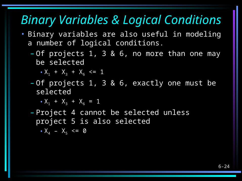
Binary Variables & Logical Conditions
• Binary variables are also useful in modeling a number of logical conditions.– Of projects 1, 3 & 6, no more than one may be
selected• X1 + X3 + X6 <= 1
– Of projects 1, 3 & 6, exactly one must be selected• X1 + X3 + X6 = 1
– Project 4 cannot be selected unless project 5 is also selected• X4 – X5 <= 0
6-25
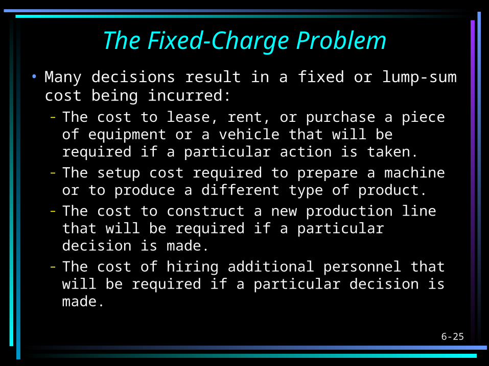
The Fixed-Charge Problem• Many decisions result in a fixed or lump-sum
cost being incurred:– The cost to lease, rent, or purchase a piece of
equipment or a vehicle that will be required if a particular action is taken.
– The setup cost required to prepare a machine or to produce a different type of product.
– The cost to construct a new production line that will be required if a particular decision is made.
– The cost of hiring additional personnel that will be required if a particular decision is made.
6-26
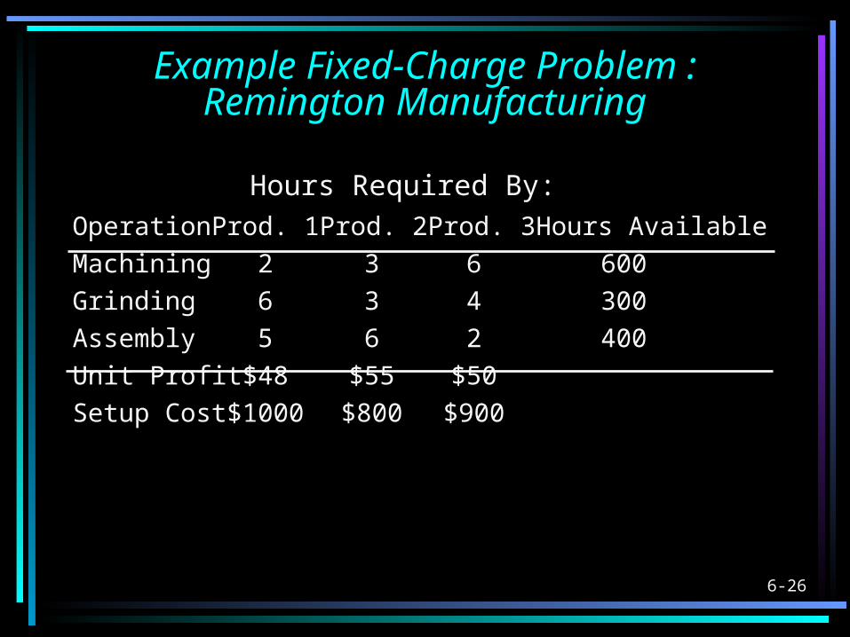
Example Fixed-Charge Problem :Remington Manufacturing
Operation Prod. 1 Prod. 2 Prod. 3Hours AvailableMachining 2 3 6 600Grinding 6 3 4 300Assembly 5 6 2 400Unit Profit $48 $55 $50Setup Cost $1000 $800 $900
Hours Required By:

6-27
Defining the Decision VariablesXi = the amount of product i to be produced, i = 1, 2, 3
3 2, 1,= 0X if 0,
0X if ,1Y i
i
ii

6-28
Defining the Objective Function
Maximize total profit.
MAX: 48X1 + 55X2 + 50X3 – 1000Y1 – 800Y2 – 900Y3
6-29
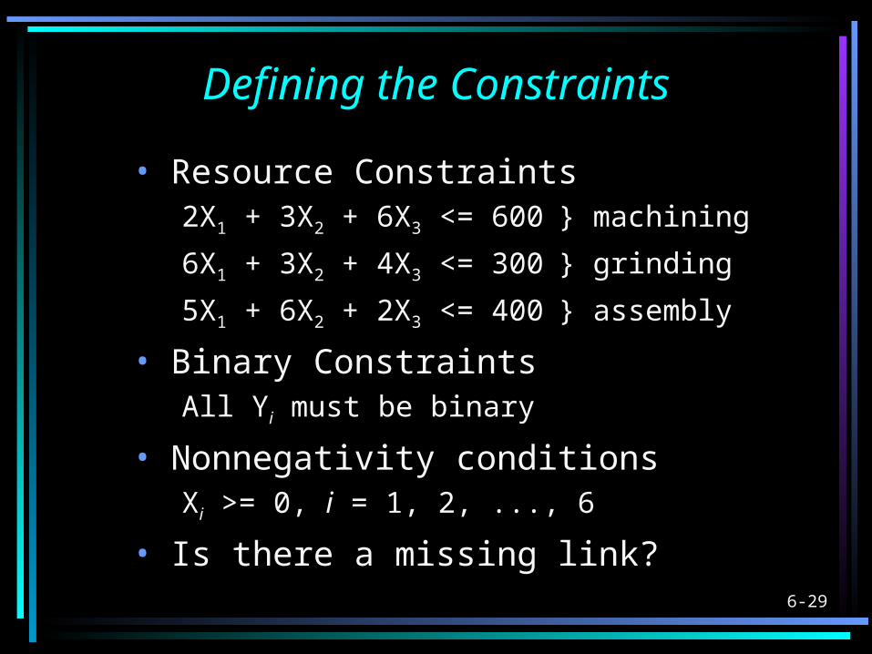
Defining the Constraints
• Resource Constraints2X1 + 3X2 + 6X3 <= 600 } machining
6X1 + 3X2 + 4X3 <= 300 } grinding
5X1 + 6X2 + 2X3 <= 400 } assembly
• Binary ConstraintsAll Yi must be binary
• Nonnegativity conditionsXi >= 0, i = 1, 2, ..., 6
• Is there a missing link?
6-30
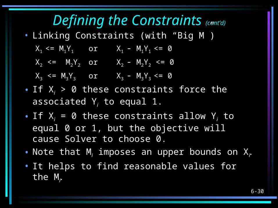
Defining the Constraints (cont’d)
• Linking Constraints (with “Big M”)X1 <= M1Y1 or X1 - M1Y1 <= 0
X2 <= M2Y2 or X2 - M2Y2 <= 0
X3 <= M3Y3 or X3 - M3Y3 <= 0
• If Xi > 0 these constraints force the associated Yi to equal 1.
• If Xi = 0 these constraints allow Yi to equal 0 or 1, but the objective will cause Solver to choose 0.
• Note that Mi imposes an upper bounds on Xi.
• It helps to find reasonable values for the Mi.

6-31
Finding Reasonable Values for M1
• Consider the resource constraints2X1 + 3X2 + 6X3 <= 600 } machining
6X1 + 3X2 + 4X3 <= 300 } grinding
5X1 + 6X2 + 2X3 <= 400 } assembly
• What is the maximum value X1 can assume? Let X2 = X3 = 0
X1 = MIN(600/2, 300/6, 400/5)
= MIN(300, 50, 80) = 50
• Maximum values for X2 & X3 can be found similarly.

6-32
MAX: 48X1 + 55X2 + 50X3 - 1000Y1 - 800Y2 - 900Y3
S.T.: 2X1 + 3X2 + 6X3 <= 600 } machining
6X1 + 3X2 + 4X3 <= 300 } grinding
5X1 + 6X2 + 2X3 <= 400 } assembly X1 - 50Y1 <= 0
X2 - 67Y2 <= 0 linking constraints
X3 - 75Y3 <= 0
All Yi must be binary
Xi >= 0, i = 1, 2, 3
Summary of the Model

6-33
Potential Pitfall• Do not use IF( ) functions to model the
relationship between the Xi and Yi.
– Suppose cell A5 represents X1
– Suppose cell A6 represents Y1
– You’ll want to let A6 = IF(A5>0,1,0)– This will not work with Solver!
• Treat the Yi just like any other variable.
– Make them changing cells.– Use the linking constraints to enforce the
proper relationship between the Xi and Yi.

6-34
Implementing the Model
See file Fig5-5.xls

6-35
Minimum Order Size RestrictionsSuppose Remington doesn’t want to manufacture any units of product 3 unless it produces at least 40 units...
Consider,
X3 <= M3Y3
X3 >= 40 Y3

6-36
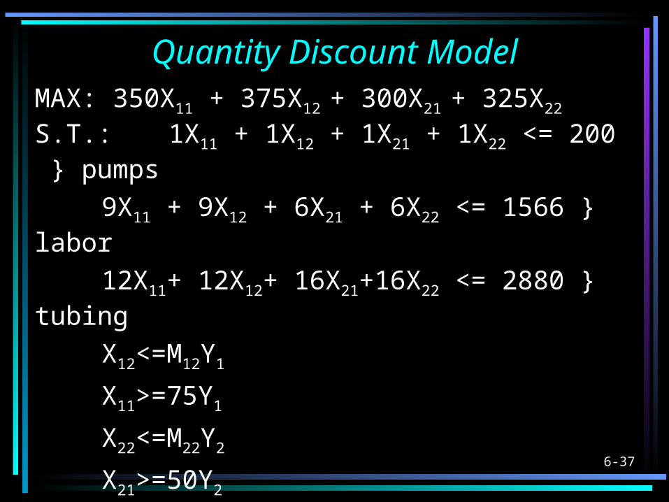
Quantity Discounts
• Assume… – If Blue Ridge Hot Tubs produces more
than 75 Aqua-Spas, it obtains discounts that increase the unit profit to $375.
– If it produces more than 50 Hydro-Luxes, the profit increases to $325.
6-37
Quantity Discount ModelMAX: 350X11 + 375X12 + 300X21 + 325X22
S.T.: 1X11 + 1X12 + 1X21 + 1X22 <= 200 } pumps
9X11 + 9X12 + 6X21 + 6X22 <= 1566 } labor
12X11+ 12X12+ 16X21+16X22 <= 2880 } tubing
X12<=M12Y1
X11>=75Y1
X22<=M22Y2
X21>=50Y2
Xij >= 0
Xij must be integers, Yi must be binary

6-38
A Contract Award Problem
• B&G Construction has 4 building projects and can purchase cement from 3 companies for the following costs:
Max.Project 1Project 2Project 3 Project 4 Supply
Co. 1 $120 $115 $130 $125 525Co. 2 $100 $150 $110 $105 450Co. 3 $140 $95 $145 $165 550Needs 450 275 300 350(tons)
Cost per Delivered Ton of Cement

6-39
A Contract Award Problem
• Side constraints:– Co. 1 will not supply orders of less than 150 tons for any project– Co. 2 can supply more than 200 tons to no more than one of the
projects– Co. 3 will accept only orders that total 200, 400, or 550 tons

6-40
Defining the Decision Variables
Xij = tons of cement purchased from company i for project j

6-41
Defining the Objective Function
Minimize total cost
MIN: 120X11 + 115X12 + 130X13 +
125X14
+ 100X21 + 150X22 + 110X23 +
105X24
+ 140X31 + 95X32 + 145X33 +
165X34

6-42
Defining the Constraints• Supply Constraints
X11 + X12 + X13 + X14 <= 525 } company 1
X21 + X22 + X23 + X24 <= 450 } company 2
X31 + X32 + X33 + X34 <= 550 } company 3
• Demand ConstraintsX11 + X21 + X31 = 450 } project 1
X12 + X22 + X32 = 275 } project 2
X13 + X23 + X33 = 300 } project 3
X14 + X24 + X34 = 350 } project 4

6-43
Implementing the Transportation Constraints
See file Fig5-6.xls

6-44
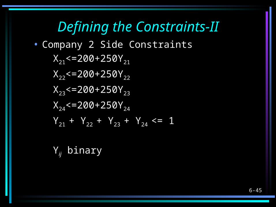
Defining the Constraints-I• Company 1 Side Constraints
X11<=525Y11
X12<=525Y12
X13<=525Y13
X14<=525Y14
X11>=150Y11
X12>=150Y12
X13>=150Y13
X14>=150Y14
Yij binary
6-45
Defining the Constraints-II• Company 2 Side Constraints
X21<=200+250Y21
X22<=200+250Y22
X23<=200+250Y23
X24<=200+250Y24
Y21 + Y22 + Y23 + Y24 <= 1
Yij binary

6-46
Defining the Constraints-III
• Company 3 Side ConstraintsX31 + X32 + X33 + X34 = 200Y31 + 400Y32 + 550Y33
Y31 + Y32 + Y33 <= 1

6-47
Implementing the Side Constraints
See file Fig5-7.xls

6-48
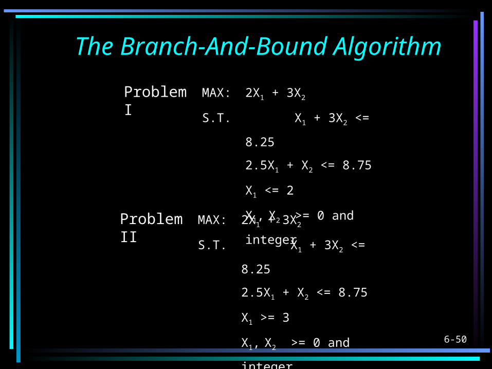
The Branch-And-Bound Algorithm
MAX: 2X1 + 3X2
S.T. X1 + 3X2 <=
8.25
2.5X1 + X2 <=
8.75
X1, X2 >= 0 and
integer

6-49
Solution to LP Relaxation
0
1
2
3
0 1 2 3 4 X1
X2
Feasible Integer Solutions
Optimal Relaxed Solution
X1 = 2.769, X2=1.826
Obj = 11.019
6-50
The Branch-And-Bound Algorithm
MAX: 2X1 + 3X2
S.T. X1 + 3X2 <= 8.25
2.5X1 + X2 <= 8.75
X1 <= 2
X1, X2 >= 0 and
integer
Problem I
MAX: 2X1 + 3X2
S.T. X1 + 3X2 <= 8.25
2.5X1 + X2 <= 8.75
X1 >= 3
X1, X2 >= 0 and
integer
Problem II

6-51
Solution to LP Relaxation
0
1
2
3
0 1 2 3 4 X1
X2
Problem I
Problem II
X1=2, X2=2.083, Obj = 10.25

6-52
The Branch-And-Bound Algorithm
MAX: 2X1 + 3X2
S.T. X1 + 3X2 <= 8.25
2.5X1 + X2 <=
8.75
X1 <= 2
X2 <= 2
X1, X2 >= 0 and
integer
Problem III
MAX: 2X1 + 3X2
S.T. X1 + 3X2 <= 8.25
2.5X1 + X2 <=
8.75
X1 <= 2
X2 >= 3
X1, X2 >= 0 and
integer
Problem IV

6-53
Solution to LP Relaxation
0
1
2
3
0 1 2 3 4 X1
X2
Problem III
Problem II
X1=2, X2=2, Obj = 10
X1=3, X2=1.25, Obj = 9.75
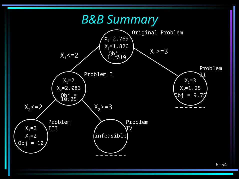
6-54
B&B SummaryX1=2.769
X2=1.826Obj = 11.019
X1=2
X2=2.083Obj = 10.25
X1=2
X2=2Obj = 10
infeasible
X1=3
X2=1.25Obj = 9.75
Original Problem
Problem IIProblem I
Problem III Problem IV
X1>=3X1<=2
X2>=3X2<=2

6-55
End of Chapter 5


