1

Wolfram Burgard, Cyrill Stachniss, Maren

Bennewitz, Giorgio Grisetti, Kai Arras

Path Planning and Collision Avoidance

Introduction toMobile Robotics

2

Motion Planning

Latombe (1991):

“…eminently necessary since, by definition, a robot accomplishes tasks by moving in the real world.”

Goals:

� Collision-free trajectories.

� Robot should reach the goal location as fast as possible.

3

… in Dynamic Environments

� How to react to unforeseen obstacles?

� efficiency

� reliability

� Dynamic Window Approaches[Simmons, 96], [Fox et al., 97], [Brock & Khatib, 99]

� Grid map based Planning[Konolige, 00]

� Nearness Diagram Navigation[Minguez at al., 2001, 2002]

� Vector-Field-Histogram+[Ulrich & Borenstein, 98]

� A*, D*, D* Lite, ARA*, …

4

Two Challenges

� Calculate the optimal path taking potential uncertainties in the actions into account

� Quickly generate actions in the case of unforeseen objects

5

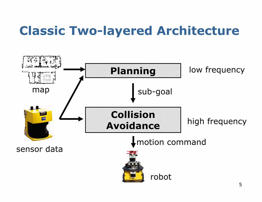
Classic Two-layered Architecture

Planning

Collision Avoidance

sensor data

map

robot

low frequency

high frequency

sub-goal

motion command

6

Dynamic Window Approach

� Collision avoidance: determine collision-free trajectories using geometric operations

� Here: robot moves on circular arcs

� Motion commands (v,ω)

� Which (v,ω) are admissible and reachable?

7

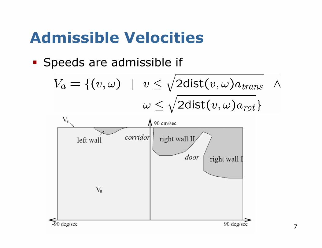
Admissible Velocities

� Speeds are admissible if

8

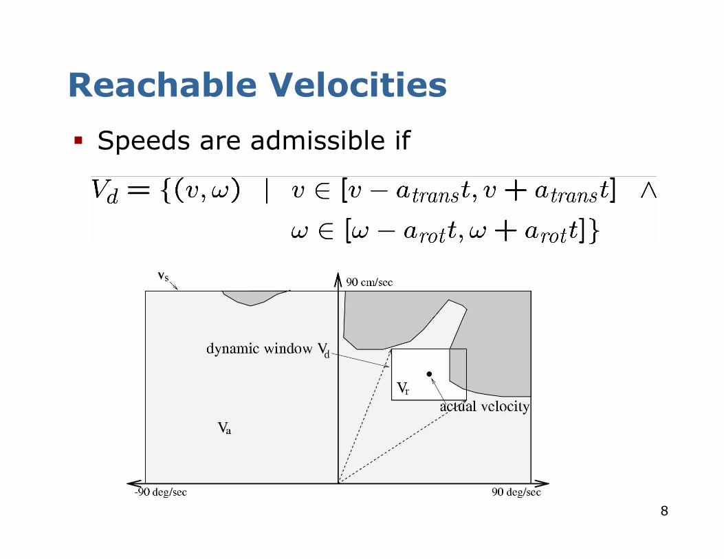
Reachable Velocities

� Speeds are admissible if

9

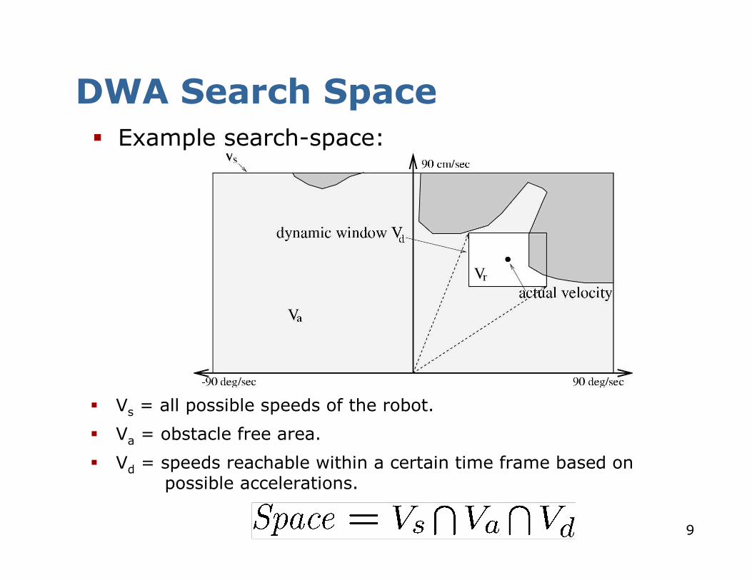
DWA Search Space

� Example search-space:

� Vs = all possible speeds of the robot.

� Va = obstacle free area.

� Vd = speeds reachable within a certain time frame based on possible accelerations.

10

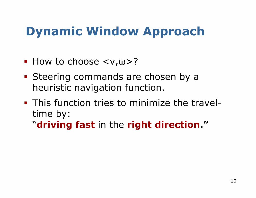
Dynamic Window Approach

� How to choose <v,ω>?

� Steering commands are chosen by a heuristic navigation function.

� This function tries to minimize the travel-time by:“driving fast in the right direction.”

11

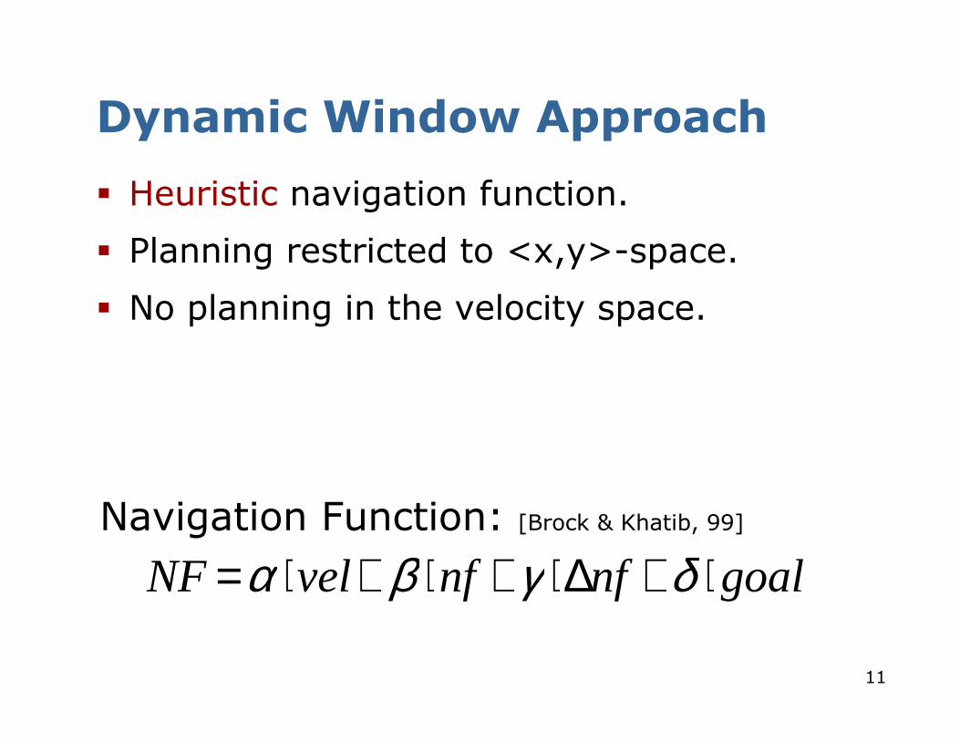
Dynamic Window Approach

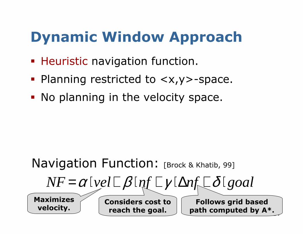
� Heuristic navigation function.

� Planning restricted to <x,y>-space.

� No planning in the velocity space.

goalnfnfvelNF ⋅+∆⋅+⋅+⋅= δγβαNavigation Function: [Brock & Khatib, 99]

12

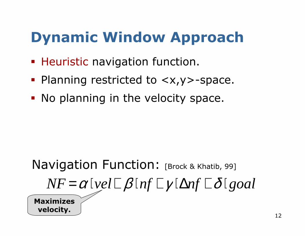
goalnfnfvelNF ⋅+∆⋅+⋅+⋅= δγβαNavigation Function: [Brock & Khatib, 99]

Maximizes velocity.

� Heuristic navigation function.

� Planning restricted to <x,y>-space.

� No planning in the velocity space.

Dynamic Window Approach

13

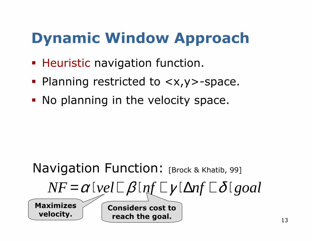
goalnfnfvelNF ⋅+∆⋅+⋅+⋅= δγβαNavigation Function: [Brock & Khatib, 99]

Considers cost to reach the goal.

Maximizes velocity.

� Heuristic navigation function.

� Planning restricted to <x,y>-space.

� No planning in the velocity space.

Dynamic Window Approach

14

goalnfnfvelNF ⋅+∆⋅+⋅+⋅= δγβαNavigation Function: [Brock & Khatib, 99]

Maximizes velocity.

Considers cost to reach the goal.

Follows grid based path computed by A*.

� Heuristic navigation function.

� Planning restricted to <x,y>-space.

� No planning in the velocity space.

Dynamic Window Approach

15

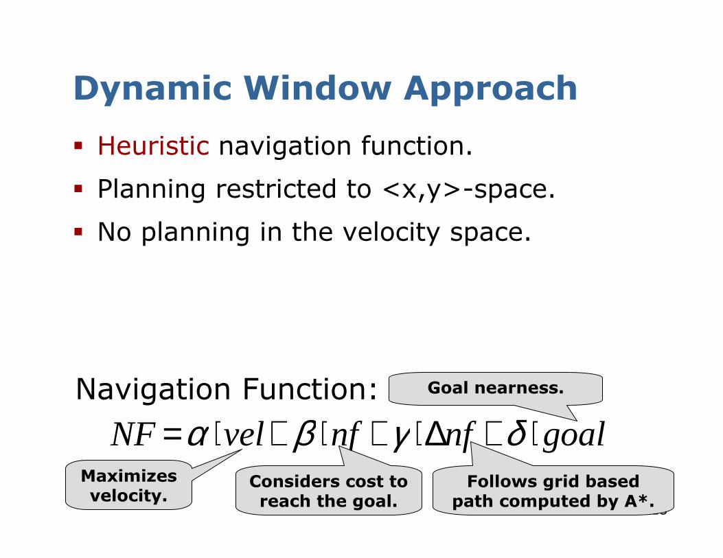
Navigation Function: [Brock & Khatib, 99]Goal nearness.

Follows grid based path computed by A*.

goalnfnfvelNF ⋅+∆⋅+⋅+⋅= δγβαMaximizes velocity.

Considers cost to reach the goal.

� Heuristic navigation function.

� Planning restricted to <x,y>-space.

� No planning in the velocity space.

Dynamic Window Approach

16

Dynamic Window Approach

� Reacts quickly.

� Low CPU power requirements.

� Guides a robot on a collision free path.

� Successfully used in a lot of real-world scenarios.

� Resulting trajectories sometimes sub-optimal.

� Local minima might prevent the robot from reaching the goal location.

17

Problems of DWAs

goalnfnfvelNF ⋅+∆⋅+⋅+⋅= δγβα

18

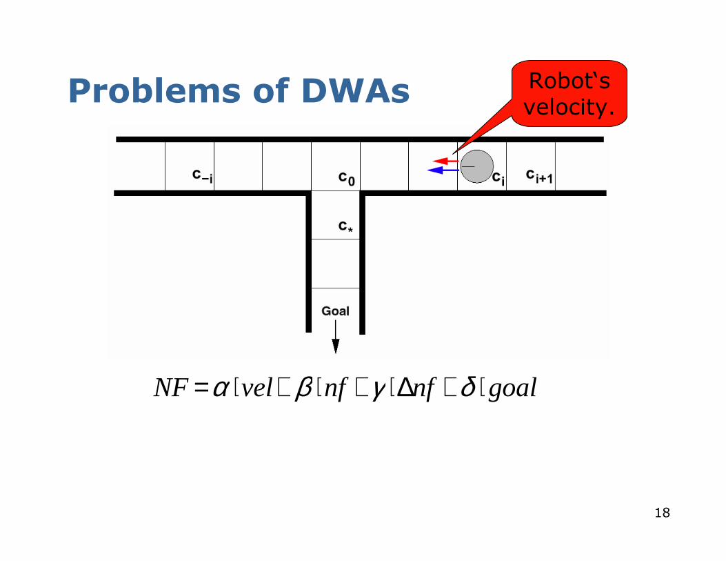
Problems of DWAs

goalnfnfvelNF ⋅+∆⋅+⋅+⋅= δγβα

Robot‘s velocity.

19

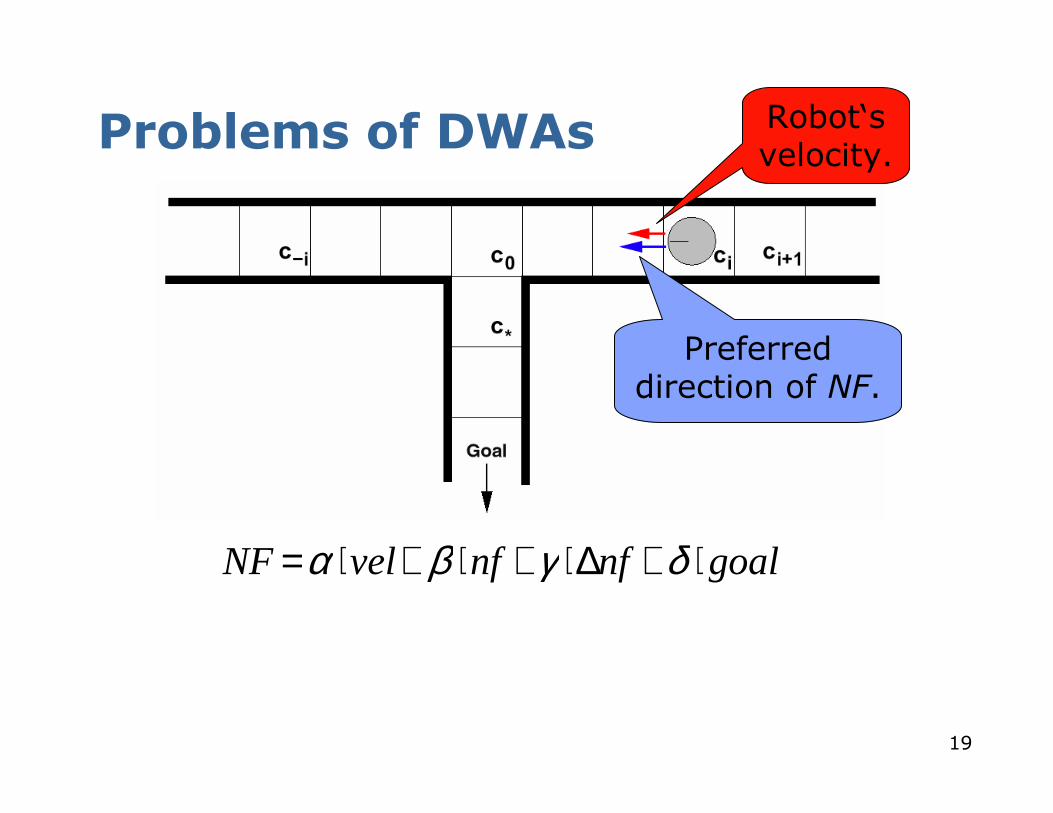
Problems of DWAs

goalnfnfvelNF ⋅+∆⋅+⋅+⋅= δγβα

Preferred direction of NF.

Robot‘s velocity.

20

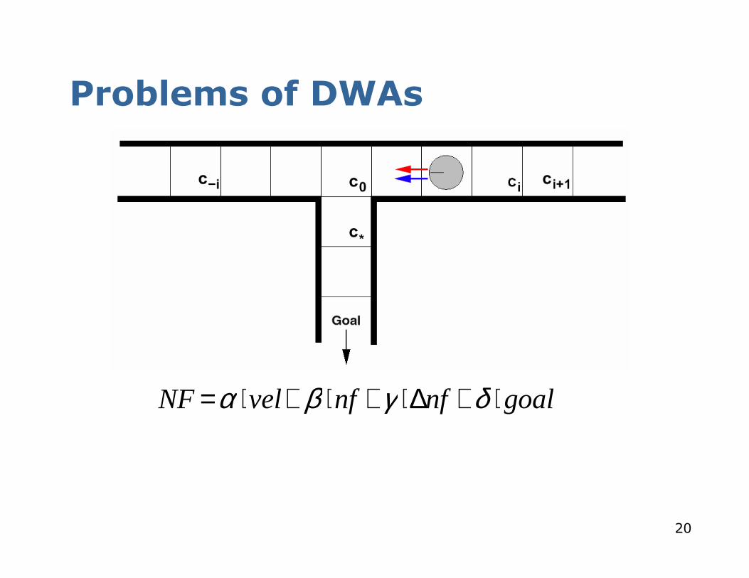
Problems of DWAs

goalnfnfvelNF ⋅+∆⋅+⋅+⋅= δγβα

21

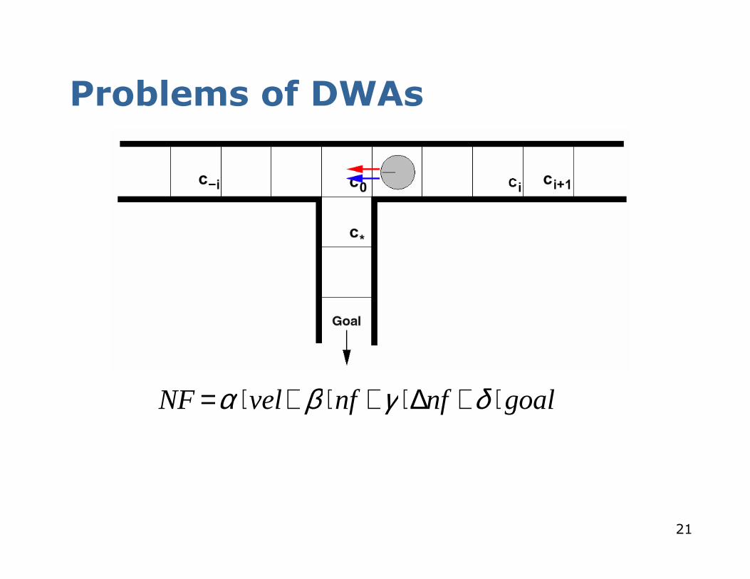
Problems of DWAs

goalnfnfvelNF ⋅+∆⋅+⋅+⋅= δγβα

22

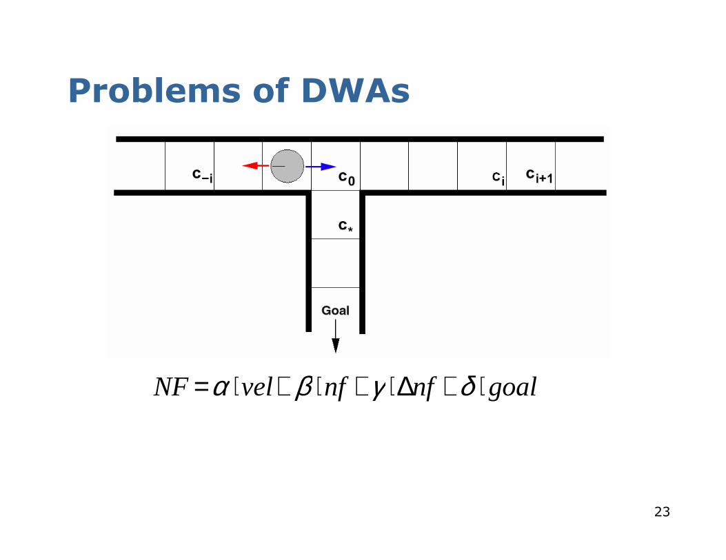
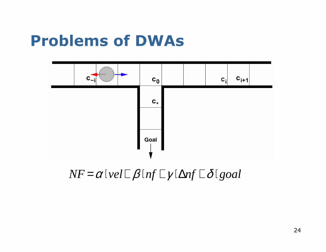
Problems of DWAs

goalnfnfvelNF ⋅+∆⋅+⋅+⋅= δγβα

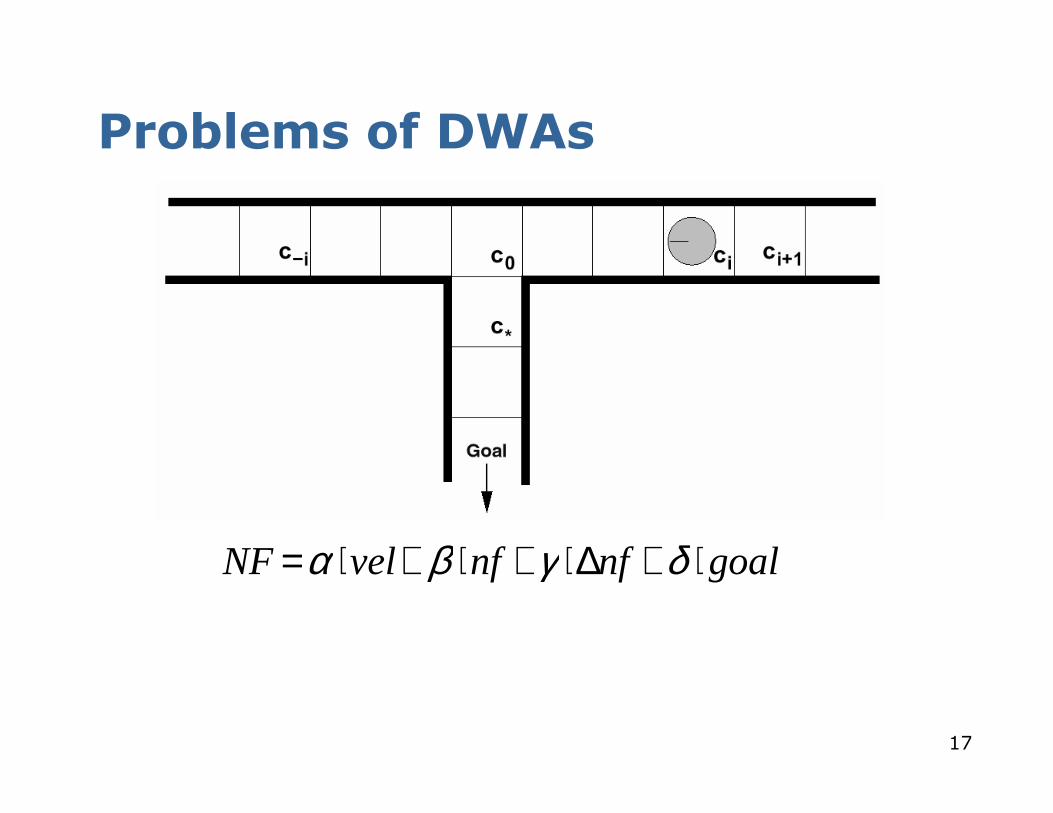
� The robot drives too fast at c0 to enter corridor facing south.

23

Problems of DWAs

goalnfnfvelNF ⋅+∆⋅+⋅+⋅= δγβα

24

Problems of DWAs

goalnfnfvelNF ⋅+∆⋅+⋅+⋅= δγβα

25

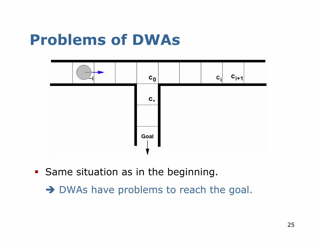
Problems of DWAs

� Same situation as in the beginning.

� DWAs have problems to reach the goal.

26

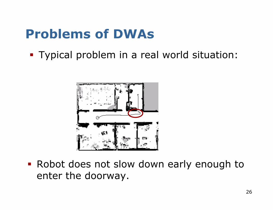
Problems of DWAs

� Typical problem in a real world situation:

� Robot does not slow down early enough to enter the doorway.

27

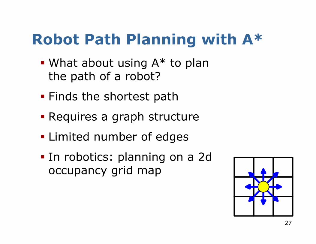
Robot Path Planning with A*

� What about using A* to plan the path of a robot?

� Finds the shortest path

� Requires a graph structure

� Limited number of edges

� In robotics: planning on a 2d occupancy grid map

28

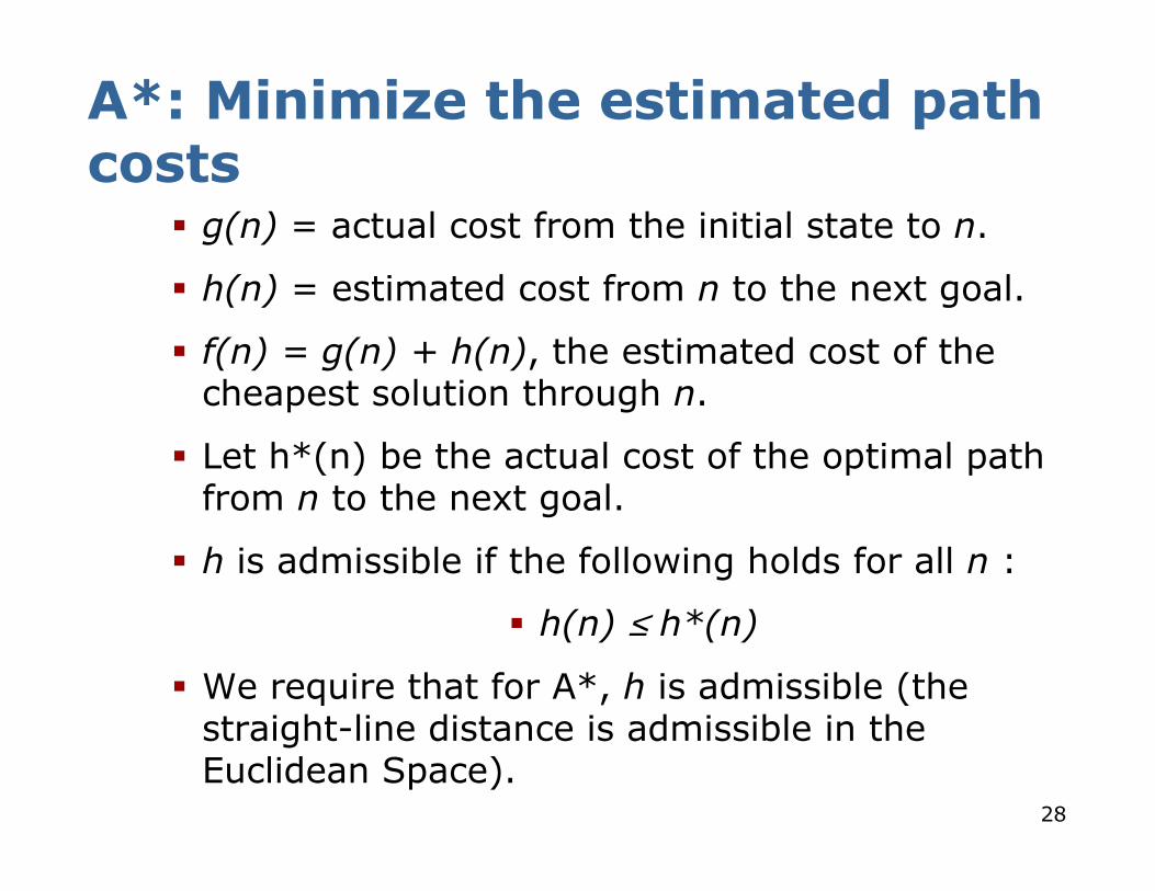
A*: Minimize the estimated path costs

� g(n) = actual cost from the initial state to n.

� h(n) = estimated cost from n to the next goal.

� f(n) = g(n) + h(n), the estimated cost of the cheapest solution through n.

� Let h*(n) be the actual cost of the optimal path from n to the next goal.

� h is admissible if the following holds for all n :

� h(n) ≤ h*(n)

� We require that for A*, h is admissible (the straight-line distance is admissible in the Euclidean Space).

29

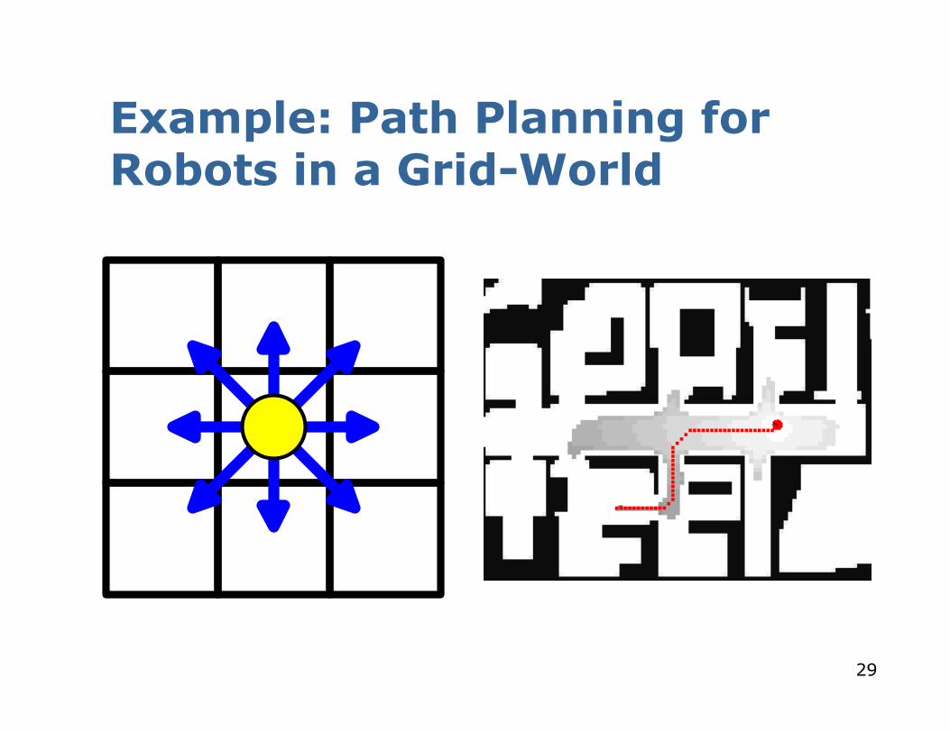
Example: Path Planning for Robots in a Grid-World

30

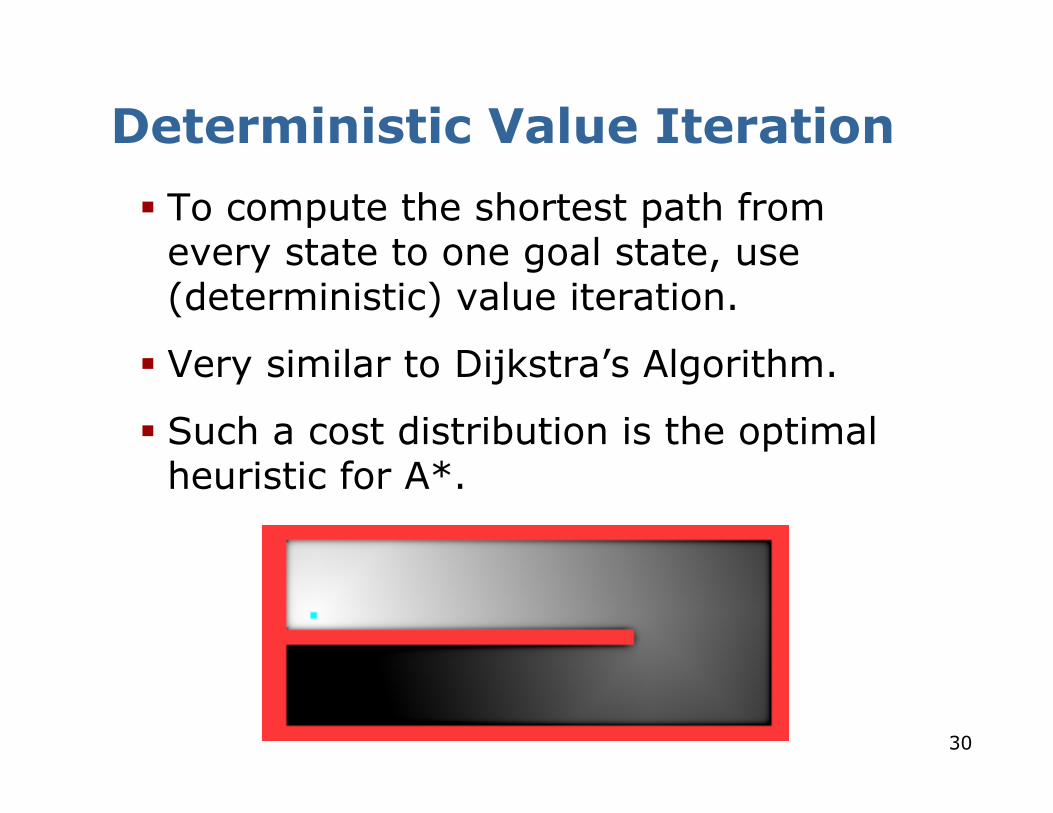
Deterministic Value Iteration

� To compute the shortest path from every state to one goal state, use (deterministic) value iteration.

� Very similar to Dijkstra’s Algorithm.

� Such a cost distribution is the optimal heuristic for A*.

31

Typical Assumption in Robotics for A* Path Planning

� A robot is assumed to be localized.

� Often a robot has to compute a path based on an occupancy grid.

� Often the correct motion commands are executed (but no perfect map).

Is this always true?

32

Problems

� What if the robot is slightly delocalized?

� Moving on the shortest path guides often the robot on a trajectory close to obstacles.

� Trajectory aligned to the grid structure.

33

Convolution of the Grid Map

� Convolution blurs the map.

� Obstacles are assumed to be bigger than in reality.

� Perform an A* search in such a convolved map.

� Robots increases distance to obstaclesand moves on a short path!

34

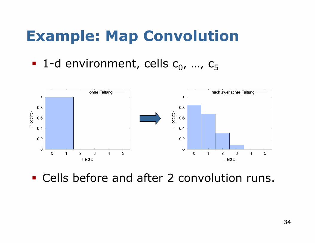
Example: Map Convolution

� 1-d environment, cells c0, …, c5

� Cells before and after 2 convolution runs.

35

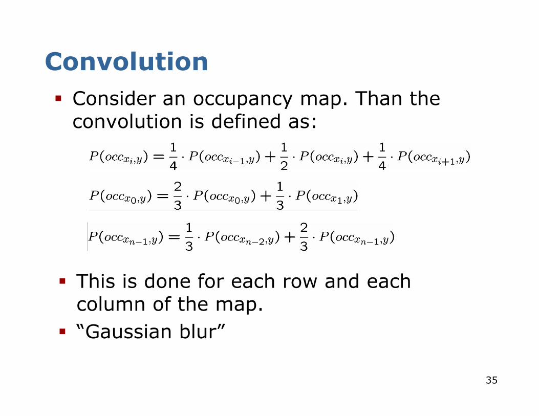
Convolution

� Consider an occupancy map. Than the convolution is defined as:

� This is done for each row and each column of the map.

� “Gaussian blur”

36

A* in Convolved Maps

� The costs are a product of path length and occupancy probability of the cells.

� Cells with higher probability (e.g., caused by convolution) are avoided by the robot.

� Thus, it keeps distance to obstacles.

� This technique is fast and quite reliable.

37

5D-Planning – an Alternative to the Two-layered Architecture

� Plans in the full <x,y,θ,v,ω>-configuration space using A*.

� considers the robot's kinematic contraints.

� Generates a sequence of steering commands to reach the goal location.

� Maximizes trade-off between driving time and distance to obstacles.

38

The Search Space (1)

� What is a state in this space?<x,y,θ,v,ω> = current position and

speed of the robot

� How does a state transition look like?<x1,y1,θ1,v1,ω1> <x2,y2,θ2,v2,ω2>

with motion command (v2,ω2) and

|v1-v2| < av, |ω1-ω2| < aω. Pose of the Robot is a result of the motion equations.

39

The Search Space (2)

Idea: search in the discretized <x,y,θ,v,ω>-space.

Problem: the search space is too huge to be explored within the time constraints (.25 secs for online control).

Solution: restrict the full search space.

40

The Main Steps of Our Algorithm

1. Update (static) grid map based on sensory input.

2. Use A* to find a trajectory in the <x,y>-space using the updated grid map.

3. Determine a restricted 5d-configuration space based on step 2.

4. Find a trajectory by planning in the restricted <x,y,θ,v,ω>-space.

41

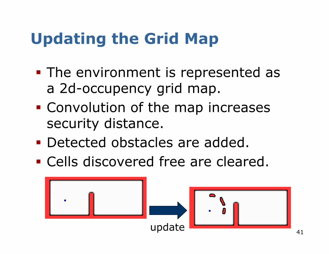
Updating the Grid Map

� The environment is represented as a 2d-occupency grid map.

� Convolution of the map increases security distance.

� Detected obstacles are added.

� Cells discovered free are cleared.

update

42

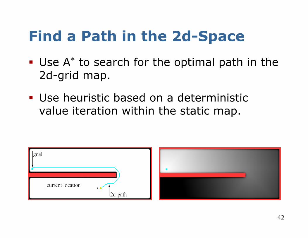
Find a Path in the 2d-Space

� Use A* to search for the optimal path in the 2d-grid map.

� Use heuristic based on a deterministic value iteration within the static map.

43

Restricting the Search Space

Assumption: the projection of the 5d-path onto the <x,y>-space lies close to the optimal 2d-path.

Therefore: construct a restricted search space (channel) based on the 2d-path.

44

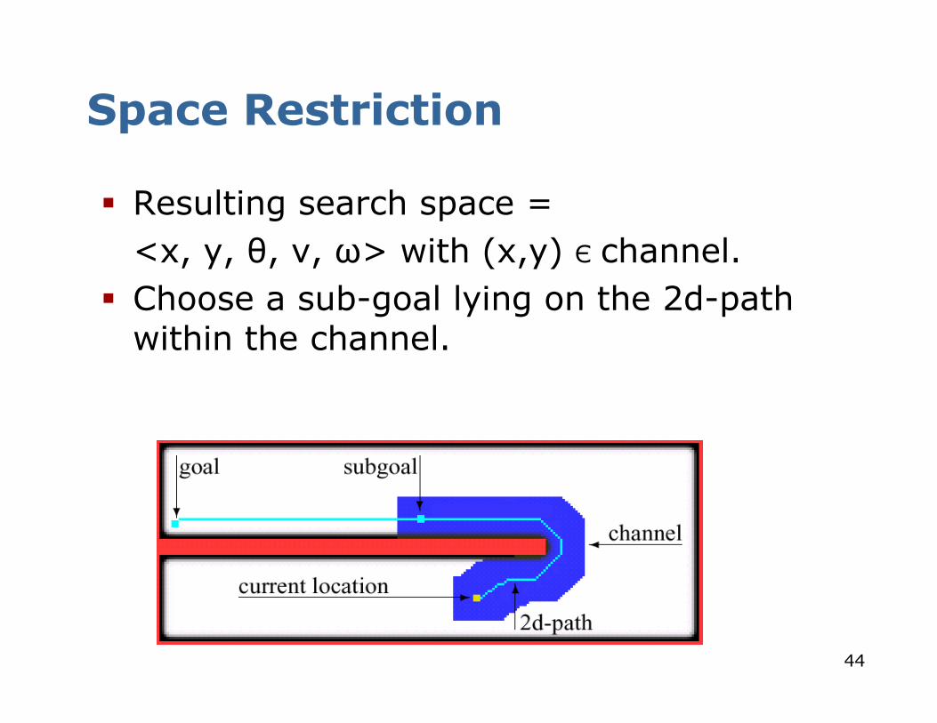
Space Restriction

� Resulting search space =

<x, y, θ, v, ω> with (x,y) Є channel.

� Choose a sub-goal lying on the 2d-path within the channel.

45

Find a Path in the 5d-Space

� Use A* in the restricted 5d-space to find a sequence of steering commands to reach the sub-goal.

� To estimate cell costs: perform a deterministic 2d-value iteration within the channel.

46

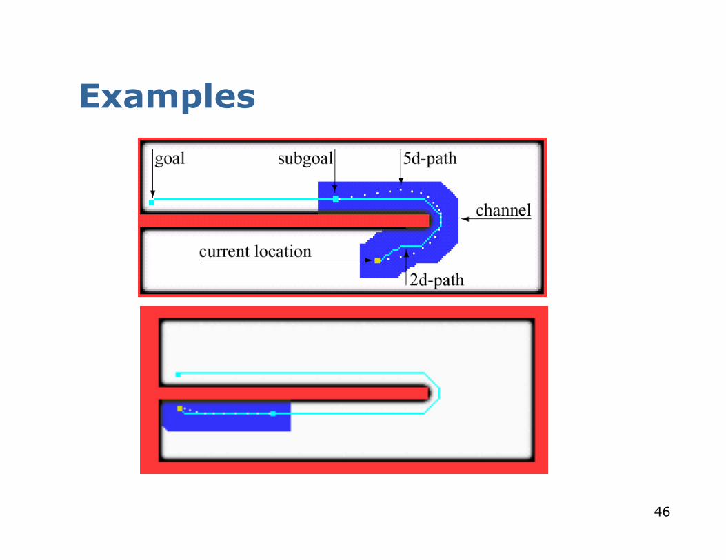
Examples

47

Timeouts

� Steering a robot online requires to set a new steering command every .25 secs.

���� Abort search after .25 secs.

How to find an admissible steering command?

48

Alternative Steering Command

� Previous trajectory still admissible? � OK

� If not, drive on the 2d-path or use DWA to find new command.

49

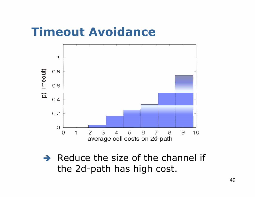
Timeout Avoidance

���� Reduce the size of the channel if the 2d-path has high cost.

50

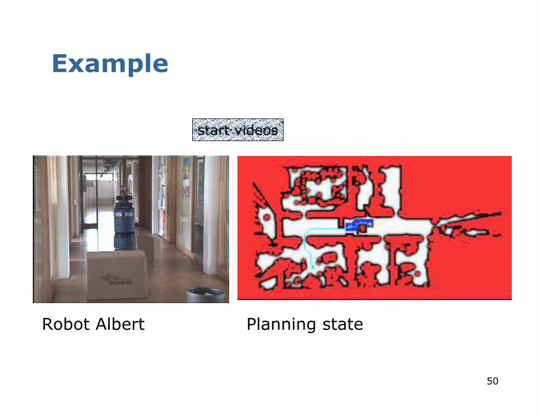
Example

Robot Albert Planning state

start videos

51

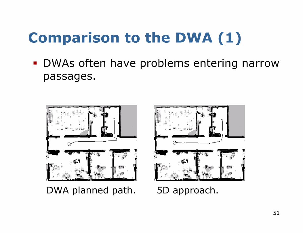
Comparison to the DWA (1)

� DWAs often have problems entering narrow passages.

DWA planned path. 5D approach.

52

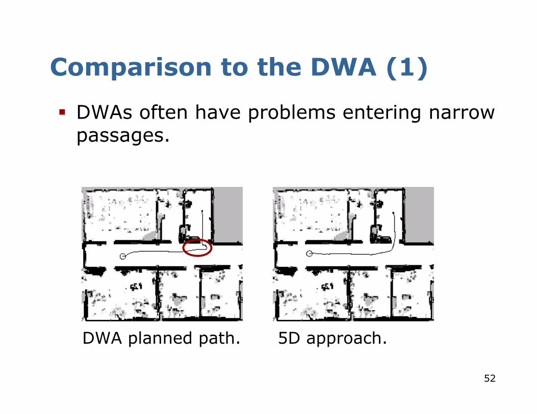
Comparison to the DWA (1)

� DWAs often have problems entering narrow passages.

DWA planned path. 5D approach.

53

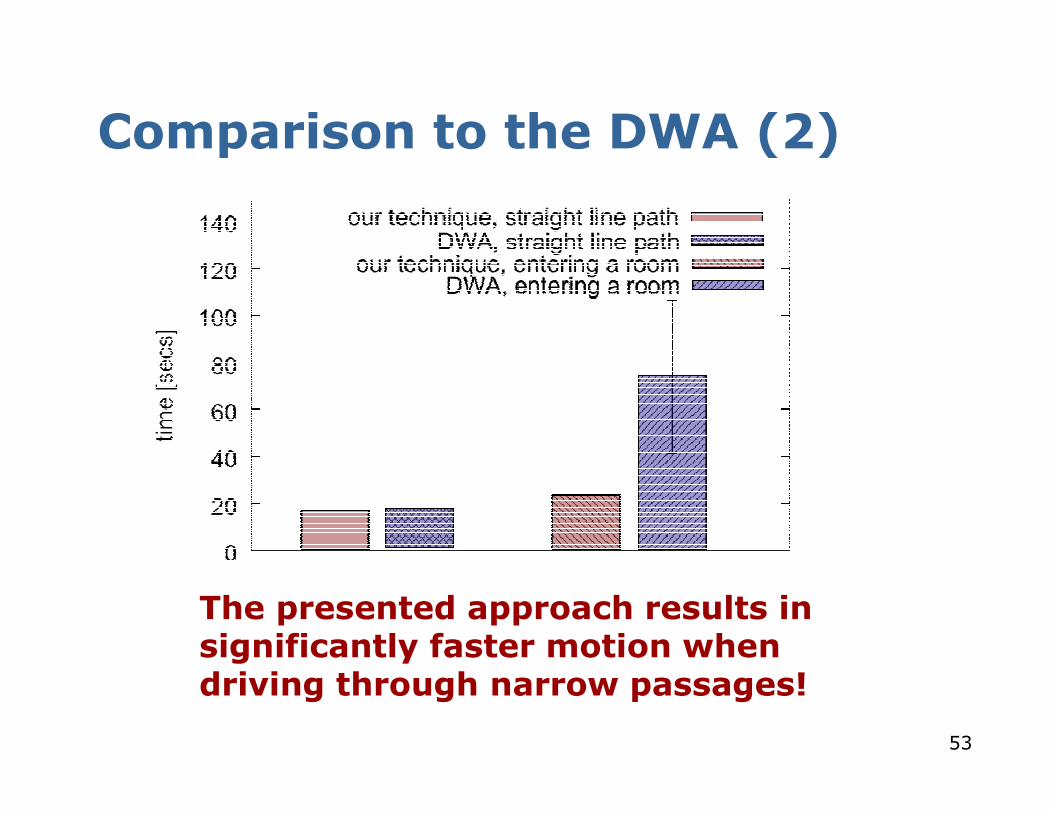
Comparison to the DWA (2)

The presented approach results in significantly faster motion when driving through narrow passages!

54

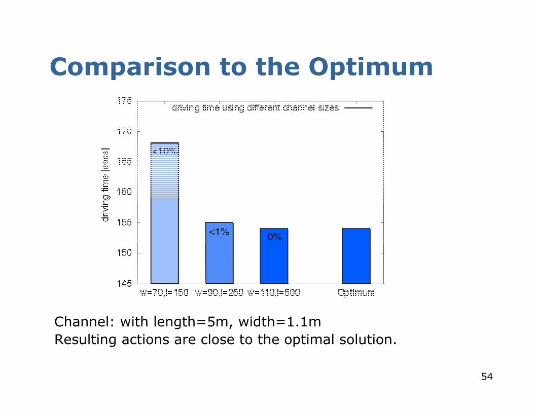
Comparison to the Optimum

Channel: with length=5m, width=1.1m

Resulting actions are close to the optimal solution.

55

Summary

� Robust navigation requires combined path planning & collision avoidance

� Approaches need to consider robot's kinematic constraints and plans in the velocity space.

� Combination of search and reactive techniques show better results than the pure DWA in a variety of situations.

� Using the 5D-approach the quality of the trajectory scales with the performance of the underlying hardware.

� The resulting paths are often close to the optimal ones.

56

What’s Missing?

� More complex vehicles (e.g., cars).

� Moving obstacles, motion prediction.

� …