INTRODUCTION TO MODERN DIGITAL HOLOGRAPHY to Modern... · 7.5 Three-dimensional holographic display...

INTRODUCTION TO MODERN DIGITAL HOLOGRAPHYWith MATLAB

Get up to speed with digital holography with this concise and straightforwardintroduction to modern techniques and conventions.Building up from the basic principles of optics, this book describes key tech-

niques in digital holography, such as phase-shifting holography, low-coherenceholography, diffraction tomographic holography, and optical scanning holography.Practical applications are discussed, and accompanied by all the theory necessaryto understand the underlying principles at work. A further chapter covers advancedtechniques for producing computer-generated holograms. Extensive MATLABcode is integrated with the text throughout and is available for download online,illustrating both theoretical results and practical considerations such as aliasing,zero padding, and sampling.Accompanied by end-of-chapter problems, and an online solutions manual

for instructors, this is an indispensable resource for students, researchers, andengineers in the fields of optical image processing and digital holography.

ting-chung poon is a Professor of Electrical and Computer Engineering atVirginia Tech, and a Visiting Professor at the Shanghai Institute of Optics and FineMechanics, Chinese Academy of Sciences. He is a Fellow of the OSA and SPIE.

jung-ping liu is a Professor in the Department of Photonics at Feng ChiaUniversity, Taiwan.

INTRODUCTION TO MODERNDIGITAL HOLOGRAPHY

With MATLAB

TING-CHUNG POONVirginia Tech, USA

JUNG-PING LIUFeng Chia University, Taiwan

University Printing House, Cambridge CB2 8BS, United Kingdom

Published in the United States of America by Cambridge University Press, New York

Cambridge University Press is part of the University of Cambridge.

It furthers the University’s mission by disseminating knowledge in the pursuit ofeducation, learning and research at the highest international levels of excellence.

www.cambridge.orgInformation on this title: www.cambridge.org/9781107016705

© T-C. Poon & J-P. Liu 2014

This publication is in copyright. Subject to statutory exceptionand to the provisions of relevant collective licensing agreements,no reproduction of any part may take place without the written

permission of Cambridge University Press.

First published 2014

Printing in the United Kingdom by TJ International Ltd. Padstow Cornwall

A catalog record for this publication is available from the British Library

Library of Congress Cataloging in Publication dataPoon, Ting-Chung.

Introduction to modern digital holography : with MATLAB / Ting-Chung Poon, Jung-Ping Liu.pages cm

ISBN 978-1-107-01670-5 (Hardback)1. Holography–Data processing. 2. Image processing–Digital techniques. I. Liu, Jung-Ping. II. Title.

TA1542.P66 2014621.36075–dc232013036072

ISBN 978-1-107-016705-Hardback

Additional resources for this publication at www.cambridge.org/digitalholography

Cambridge University Press has no responsibility for the persistence or accuracy ofURLs for external or third-party internet websites referred to in this publication,and does not guarantee that any content on such websites is, or will remain,

accurate or appropriate.

http://www.cambridge.org/9781107016705

http://www.cambridge.org

http://www.cambridge.org/digitalholography

Contents

Preface page ix

1 Wave optics 11.1 Maxwell’s equations and the wave equation 11.2 Plane waves and spherical waves 31.3 Scalar diffraction theory 5

1.3.1 Fresnel diffraction 91.3.2 Fraunhofer diffraction 11

1.4 Ideal thin lens as an optical Fourier transformer 141.5 Optical image processing 15Problems 24References 26

2 Fundamentals of holography 272.1 Photography and holography 272.2 Hologram as a collection of Fresnel zone plates 282.3 Three-dimensional holographic imaging 33

2.3.1 Holographic magnifications 382.3.2 Translational distortion 392.3.3 Chromatic aberration 40

2.4 Temporal and spatial coherence 422.4 1 Temporal coherence 432.4.2 Coherence time and coherence length 452.4.3 Some general temporal coherence considerations 462.4.4 Fourier transform spectroscopy 482.4.5 Spatial coherence 512.4.6 Some general spatial coherence considerations 53

Problems 56References 58

v

3 Types of holograms 593.1 Gabor hologram and on-axis (in-line) holography 593.2 Off-axis holography 613.3 Image hologram 643.4 Fresnel and Fourier holograms 68

3.4.1 Fresnel hologram and Fourier hologram 683.4.2 Lensless Fourier hologram 70

3.5 Rainbow hologram 73Problems 78References 78

4 Conventional digital holography 794.1 Sampled signal and discrete Fourier transform 794.2. Recording and limitations of the image sensor 89

4.2.1 Imager size 914.2.2 Pixel pitch 914.2.3 Modulation transfer function 92

4.3 Digital calculations of scalar diffraction 954.3.1 Angular spectrum method (ASM) 954.3.2 Validity of the angular spectrum method 974.3.3 Fresnel diffraction method (FDM) 994.3.4 Validation of the Fresnel diffraction method 1014.3.5 Backward propagation 103

4.4 Optical recording of digital holograms 1054.4 1 Recording geometry 1054.4 2 Removal of the twin image and the zeroth-order light 108

4.5 Simulations of holographic recording and reconstruction 111Problems 116References 117

5 Digital holography: special techniques 1185.1 Phase-shifting digital holography 118

5.1.1 Four-step phase-shifting holography 1195.1.2 Three-step phase-shifting holography 1205.1.3 Two-step phase-shifting holography 1205.1.4 Phase step and phase error 1225.1.5 Parallel phase-shifting holography 124

5.2 Low-coherence digital holography 1265.3 Diffraction tomographic holography 1335.4 Optical scanning holography 137

vi Contents

5.4.1 Fundamental principles 1385.4.2 Hologram construction and reconstruction 1425.4.3 Intuition on optical scanning holography 144


6 Applications in digital holography 1516.1 Holographic microscopy 151

6.1.1 Microscope-based digital holographic microscopy 1516.1.2 Fourier-based digital holographic microscopy 1546.1.3 Spherical-reference-based digital holographic

microscopy 1566.2 Sectioning in holography 1586.3 Phase extraction 1646.4 Optical contouring and deformation measurement 168

6.4.1 Two-wavelength contouring 1696.4.2 Two-illumination contouring 1726.4.3 Deformation measurement 175


7 Computer-generated holography 1797.1 The detour-phase hologram 1797.2 The kinoform hologram 1857.3 Iterative Fourier transform algorithm 1877.4 Modern approach for fast calculations and holographic

information processing 1897.4.1 Modern approach for fast calculations 1897.4.2 Holographic information processing 196

7.5 Three-dimensional holographic display using spatial lightmodulators 1997.5.1 Resolution 1997.5.2 Digital mask programmable hologram 2017.5.3 Real-time display 2057.5.4 Lack of SLMs capable of displaying a complex function 206


Index 214

Contents vii

Preface

Owing to the advance in faster electronics and digital processing power, the pastdecade has seen an impressive re-emergence of digital holography. Digitalholography is a topic of growing interest and it finds applications in three-dimensional imaging, three-dimensional displays and systems, as well as bio-medical imaging and metrology. While research in digital holography continuesto be vibrant and digital holography is maturing, we find that there is a lack oftextbooks in the area. The present book tries to serve this need: to promote andteach the foundations of digital holography. In addition to presenting traditionaldigital holography and applications in Chapters 1–4, we also discuss modernapplications and techniques in digital holography such as phase-shifting holog-raphy, low-coherence holography, diffraction tomographic holography, opticalscanning holography, sectioning in holography, digital holographic microscopyas well as computer-generated holography in Chapters 5–7. This book is gearedtowards undergraduate seniors or first-year graduate-level students in engineer-ing and physics. The material covered is suitable for a one-semester course inFourier optics and digital holography. The book is also useful for scientists andengineers, and for those who simply want to learn about optical image processingand digital holography.

We believe in the inclusion of MATLAB® in the textbook because digitalholography relies heavily on digital computations to process holographic data.MATLAB® will help the reader grasp and visualize some of the importantconcepts in digital holography. The use of MATLAB® not only helps to illustratethe theoretical results, but also makes us aware of computational issues such asaliasing, zero padding, sampling, etc. that we face in implementing them. Never-theless, this text is not about teaching MATLAB®, and some familiarity withMATLAB® is required to understand the codes.

ix

Ting-Chung Poon would like to thank his wife, Eliza, and his children, Christinaand Justine, for their love. This year is particularly special to him as Christina gavebirth to a precious little one – Gussie. Jung-Ping Liu would like to thank his wife,Hui-Chu, and his parents for their understanding and encouragement.

x Preface

1

Wave optics

1.1 Maxwell’s equations and the wave equation

In wave optics, we treat light as waves. Wave optics accounts for wave effects suchas interference and diffraction. The starting point for wave optics is Maxwell’sequations:

r�D ¼ ρv, ð1:1Þr�B ¼ 0, ð1:2Þ

r � E ¼ −∂B∂t

, ð1:3Þ

r �H ¼ J ¼ JC þ ∂D∂t

, ð1:4Þ

where we have four vector quantities called electromagnetic (EM) fields: theelectric field strength E (V/m), the electric flux density D (C/m2), the magneticfield strength H (A/m), and the magnetic flux density B (Wb/m2). The vectorquantity JC and the scalar quantity ρv are the current density (A/m2) and theelectric charge density (C/m3), respectively, and they are the sources responsiblefor generating the electromagnetic fields. In order to determine the four fieldquantities completely, we also need the constitutive relations

D ¼ εE, ð1:5Þand

B ¼ μH, ð1:6Þ

where ε and μ are the permittivity (F/m) and permeability (H/m) of the medium,respectively. In the case of a linear, homogenous, and isotropic medium such as invacuum or free space, ε and μ are scalar constants. Using Eqs. (1.3)–(1.6), we can

1

derive a wave equation in E or B in free space. For example, by taking the curl ofE in Eq. (1.3), we can derive the wave equation in E as

r2E− με∂2E∂t2

¼ μ∂JC∂t

þ 1εrρv, ð1:7Þ

where r2 ¼ ∂2/∂x2 þ ∂2/∂y2 þ ∂2/∂z2 is the Laplacian operator in Cartesiancoordinates. For a source-free medium, i.e., JC ¼ 0 and ρν ¼ 0, Eq. (1.7) reduces tothe homogeneous wave equation:

r2E−1v2∂2E∂t2

¼ 0: ð1:8Þ

Note that v ¼ 1=ffiffiffiffiffiμε

pis the velocity of the wave in the medium. Equation (1.8) is

equivalent to three scalar equations, one for every component of E. Let

E ¼ Exax þ Eyay þ Ezaz, ð1:9Þ

where ax, ay, and az are the unit vectors in the x, y, and z directions, respectively.Equation (1.8) then becomes

∂2

∂x2þ ∂2

∂y2þ ∂2

∂z2

� �ðExax þ Eyay þ EzazÞ ¼ 1

v2∂2

∂t2ðExax þ Eyay þ EzazÞ: ð1:10Þ

Comparing the ax-component on both sides of the above equation gives us

∂2Ex

∂x2þ ∂2Ex

∂y2þ ∂2Ex

∂z2¼ 1

v2∂2Ex

∂t2:

Similarly, we can derive the same type of equation shown above for the Ey and Ez

components by comparison with other components in Eq. (1.10). Hence we canwrite a compact equation for the three components as

∂2ψ∂x2

þ ∂2ψ∂y2

þ ∂2ψ∂z2

¼ 1v2

∂2ψ∂t2

ð1:11aÞ

or

r2ψ ¼ 1v2∂2ψ∂t2

, ð1:11bÞ

where ψ can represent a component, Ex, Ey, or Ez, of the electric field E. Equation(1.11) is called the three-dimensional scalar wave equation. We shall look at someof its simplest solutions in the next section.

2 Wave optics

1.2 Plane waves and spherical waves

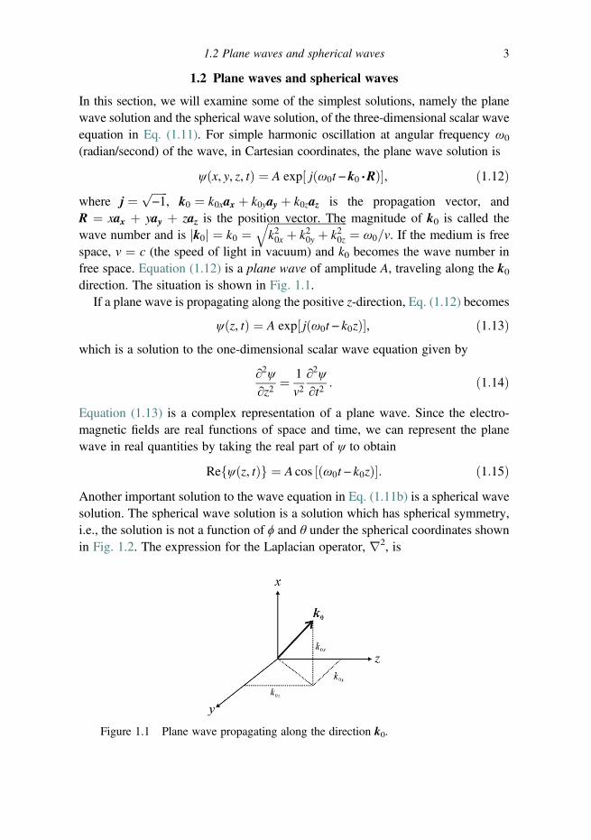
In this section, we will examine some of the simplest solutions, namely the planewave solution and the spherical wave solution, of the three-dimensional scalar waveequation in Eq. (1.11). For simple harmonic oscillation at angular frequency ω0

(radian/second) of the wave, in Cartesian coordinates, the plane wave solution is

ψðx, y, z, tÞ ¼ A exp½ jðω0t − k0�RÞ�, ð1:12Þwhere j ¼ ffiffiffiffiffiffi

−1p

, k0 ¼ k0xax þ k0yay þ k0zaz is the propagation vector, andR ¼ xax þ yay þ zaz is the position vector. The magnitude of k0 is called thewave number and is jk0j ¼ k0 ¼

ffiffiffiffiffiffiffiffiffiffiffiffiffiffiffiffiffiffiffiffiffiffiffiffiffiffiffiffiffik20x þ k20y þ k20z

q¼ ω0=v. If the medium is free

space, ν ¼ c (the speed of light in vacuum) and k0 becomes the wave number infree space. Equation (1.12) is a plane wave of amplitude A, traveling along the k0direction. The situation is shown in Fig. 1.1.

If a plane wave is propagating along the positive z-direction, Eq. (1.12) becomes

ψðz, tÞ ¼ A exp½ jðω0t − k0zÞ�, ð1:13Þwhich is a solution to the one-dimensional scalar wave equation given by

∂2ψ∂z2

¼ 1v2∂2ψ∂t2

: ð1:14Þ

Equation (1.13) is a complex representation of a plane wave. Since the electro-magnetic fields are real functions of space and time, we can represent the planewave in real quantities by taking the real part of ψ to obtain

Refψðz, tÞg ¼ A cos ½ðω0t − k0zÞ�: ð1:15ÞAnother important solution to the wave equation in Eq. (1.11b) is a spherical wavesolution. The spherical wave solution is a solution which has spherical symmetry,i.e., the solution is not a function of ϕ and θ under the spherical coordinates shownin Fig. 1.2. The expression for the Laplacian operator, r2, is

Figure 1.1 Plane wave propagating along the direction k0.

1.2 Plane waves and spherical waves 3

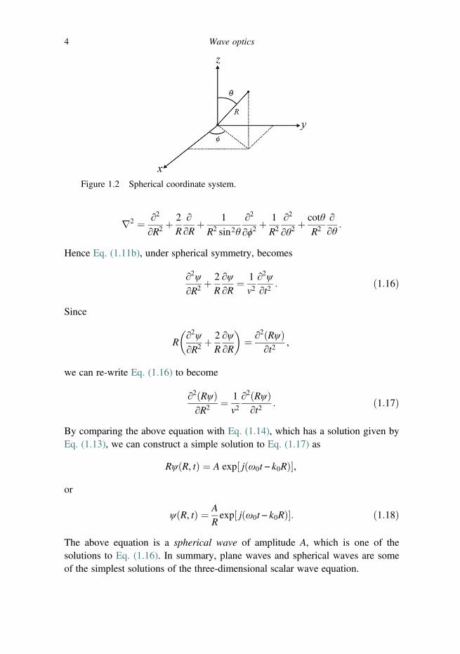
r2 ¼ ∂2

∂R2 þ2R

∂∂R

þ 1

R2 sin2θ

∂2

∂ϕ2þ 1

R2

∂2

∂θ2þ cotθ

R2

∂∂θ

:

Hence Eq. (1.11b), under spherical symmetry, becomes

∂2ψ

∂R2 þ2R

∂ψ∂R

¼ 1v2∂2ψ∂t2

: ð1:16Þ

Since

R∂2ψ

∂R2 þ2R

∂ψ∂R

� �¼ ∂2ðRψÞ

∂t2,

we can re-write Eq. (1.16) to become

∂2ðRψÞ∂R2 ¼ 1

v2∂2ðRψÞ∂t2

: ð1:17Þ

By comparing the above equation with Eq. (1.14), which has a solution given byEq. (1.13), we can construct a simple solution to Eq. (1.17) as

Rψ R, tð Þ ¼ A exp j ω0t − k0Rð Þ½ �,

or

ψ R, tð Þ ¼ A

Rexp j ω0t − k0Rð Þ½ �: ð1:18Þ

The above equation is a spherical wave of amplitude A, which is one of thesolutions to Eq. (1.16). In summary, plane waves and spherical waves are someof the simplest solutions of the three-dimensional scalar wave equation.

Figure 1.2 Spherical coordinate system.

4 Wave optics

1.3 Scalar diffraction theory

For a plane wave incident on an aperture or a diffracting screen, i.e., an opaquescreen with some openings allowing light to pass through, we need to find the fielddistribution exiting the aperture or the diffracted field. To tackle the diffractionproblem, we find the solution of the scalar wave equation under some initialcondition. Let us assume the aperture is represented by a transparency withamplitude transmittance, often called transparency function, given by t(x, y),located on the plane z = 0 as shown in Fig. 1.3.

A plane wave of amplitude A is incident on the aperture. Hence at z ¼ 0,according to Eq. (1.13), the plane wave immediately in front of the apertureis given by A exp( jω0t). The field distribution immediately after the aperture isψ(x, y, z ¼ 0, t) ¼ At(x, y) exp( jω0t). In general, t(x, y) is a complex function thatmodifies the field distribution incident on the aperture, and the transparency hasbeen assumed to be infinitely thin. To develop ψ(x, y, z ¼ 0, t) further mathematic-ally, we write

ψ x, y, z ¼ 0, tð Þ ¼ At x, yð Þexp jω0tð Þ ¼ ψp x, y; z ¼ 0ð Þexp jω0tð Þ¼ ψp0 x, yð Þexp jω0tð Þ: ð1:19Þ

The quantity ψp0(x, y) is called the complex amplitude in optics. This complexamplitude is the initial condition, which is given by ψp0(x, y) ¼ A � t(x, y), theamplitude of the incident plane wave multiplied by the transparency function ofthe aperture. To find the field distribution at z away from the aperture, we modelthe solution in the form of

ψðx, y, z, tÞ ¼ ψpðx, y; zÞexpð jω0tÞ, ð1:20Þwhere ψp (x, y; z) is the unknown to be found with initial condition ψp0(x, y) given.To find ψp(x, y; z), we substitute Eq. (1.20) into the three-dimensional scalar waveequation given by Eq. (1.11a) to obtain the Helmholtz equation for ψp(x, y; z),

Figure 1.3 Diffraction geometry: t(x, y) is a diffracting screen.

1.3 Scalar diffraction theory 5

∂2ψp

∂x2þ ∂2ψp

∂y2þ ∂2ψp

∂z2þ k20ψp ¼ 0: ð1:21Þ

To find the solution to the above equation, we choose to use the Fourier transformtechnique. The two-dimensional Fourier transform of a spatial signal f(x, y) isdefined as

F f f ðx, yÞg ¼ Fðkx, kyÞ ¼ðð∞−∞

f ðx, yÞexpð jkxxþ jkyyÞdx dy, ð1:22aÞ

and the inverse Fourier transform is

F −1fFðkx, kyÞg ¼ f ðx, yÞ ¼ 14π2

ðð∞−∞

Fðkx, kyÞexpð− jkxx− jkyyÞdkx dky, ð1:22bÞ

where kx and ky are called spatial radian frequencies as they have units of radianper unit length. The functions f(x, y) and F(xx, ky) form a Fourier transform pair.Table 1.1 shows some of the most important transform pairs.

By taking the two-dimensional Fourier transform of Eq. (1.21) and usingtransform pair number 4 in Table 1.1 to obtain

F

�∂2ψp

∂x2

�¼ ð− jkxÞ2Ψpðkx, ky; zÞ

F

�∂2ψp

∂y2

�¼ ð− jkyÞ2Ψpðkx, ky; zÞ,

ð1:23Þ

where F fψp x, y; zð Þg ¼ Ψp kx, ky; z� �

, we have a differential equation in Ψp(kx, ky; z)given by

d2Ψp

dz2þ k20 1−

k2xk20

−k2yk20

!Ψp ¼ 0 ð1:24Þ

subject to the initial known condition F fψp x, y; z ¼ 0ð Þg ¼ Ψp kx, ky; z ¼ 0� � ¼

Ψp0 kx, ky� �

. The solution to the above second ordinary different equation isstraightforward and is given by

Ψpðkx, ky; zÞ ¼ Ψp0ðkx, kyÞexp − jk0ffiffiffiffiffiffiffiffiffiffiffiffiffiffiffiffiffiffiffiffiffiffiffiffiffiffiffiffiffiffiffiffiffiffiffiffiffið1− k2x=k20 − k2y=k20Þ

qz

h ið1:25Þ

as we recognize that the differential equation of the form

d2yðzÞdz2

þ α2yðzÞ ¼ 0

6 Wave optics

Table 1.1 Fourier transform pairs

1.f(x, y) F(kx, ky)

2. Shiftingf(x − x0, y − y0) F(kx, ky) exp( jkxx0 þ jkyy0)

3. Scaling

f(ax, by)1

jabj fkxa,kyb

� �4. Differentiation

∂f(x, y) / ∂x −jkxF kx, ky� �

5. Convolution integral

f 1 � 2 ¼ðð∞−∞

f 1ðx0, y0Þf 2ðx−x0, y−y0Þdx0dy0Product of spectra

F1ðkx, kyÞF2ðkx, kyÞwhere F f f 1ðx, yÞg ¼ F1ðkx, kyÞ andF f f 2ðx, yÞg ¼ F2ðkx, kyÞ

6. Correlation

f 1� f 2¼ðð∞−∞

f �1ðx0,y0Þf 2ðxþx0,yþy0Þdx0dy0 F�1ðkx, kyÞF2ðkx, kyÞ

7. Gaussian function

exp½−αðx2 þ y2Þ�Gaussian function

παexp −

ðk2x þ k2xÞ4α

8. Constant of unity

1

Delta function

4π2δðx,yÞ¼ðð−∞∞

1expð�jkxx� jkyyÞdkx dky

9. Delta functionδðx, yÞ

Constant of unity1

10. Triangular function

Λx

a,y

b

� �¼ Λ

x

a

� �Λ

y

b

� �

where Λx

a

� �¼(1− xa

for xa

� 1

0 otherwise

a sinc2kxa

2π

� �b sinc2

kyb

2π

� �

11. Rectangular function

rectðx, yÞ ¼ rect xð ÞrectðyÞ

where rectðxÞ ¼n 1 for jxj < 1=20 otherwise

Sinc function

sinckx2π

,ky2π

� �¼ sinc

kx2π

� �sinc

ky2π

� �,

where sinc(x) ¼ sin(πx)/πx

12. Linear phase (plane wave)exp½−jðaxþ byÞ� 4π2δ(kx − a, ky − b)

13. Quadratic phase (complex Fresnelzone plate CFZP)

exp½−jaðx2 þ y2Þ�

Quadratic phase (complex Fresnel zoneplate CFZP)

−jπa

expj

4aðk2x þ k2yÞ

has the solution given by

yðzÞ ¼ yð0Þexp½− jαz�:From Eq. (1.25), we define the spatial frequency transfer function of propagationthrough a distance z as [1]

H ðkx, ky; zÞ ¼ Ψpðkx, ky; zÞ=Ψp0ðkx, kyÞ¼ exp − jk0

ffiffiffiffiffiffiffiffiffiffiffiffiffiffiffiffiffiffiffiffiffiffiffiffiffiffiffiffiffiffiffiffiffiffiffiffiffi�1− k2x=k

20 − k

2y=k

20

�qz

h i:

ð1:26Þ

Hence the complex amplitude ψp(x, y; z) is given by the inverse Fourier transformof Eq. (1.25):

ψpðx,y;zÞ¼F −1fΨpðkx,ky;zÞg¼F −1fΨp0ðkx,kyÞH ðkx,ky;zÞg

¼ 14π2

ðð−∞∞

Ψp0ðkx,kyÞexp − jk0ffiffiffiffiffiffiffiffiffiffiffiffiffiffiffiffiffiffiffiffiffiffiffiffiffiffiffiffiffiffiffiffiffiffi�1−k2x=k

20−k

2y=k

20

�qz

h iexpð−jkxx−jkyyÞdkx dky:

ð1:27ÞThe above equation is a very important result. For a given field distribution alongthe z ¼ 0 plane, i.e., ψp (x, y; z ¼ 0) ¼ ψp0(x, y), we can find the field distributionacross a plane parallel to the (x, y) plane but at a distance z from it by calculatingEq. (1.27). The term Ψp0(kx, ky) is a Fourier transform of ψp0(x, y) according toEq. (1.22):

ψp0ðx,yÞ ¼ F −1fΨp0ðkx,kyÞg¼ 14π2

ðð∞−∞

Ψp0ðkx,kyÞexpð− jkxx− jkyyÞdkx dky: ð1:28Þ

The physical meaning of the above integral is that we first recognize a plane wavepropagating with propagation vector k0, as illustrated in Fig. 1.1. The complexamplitude of the plane wave, according to Eq. (1.12), is given by

A expð− jk0xx− jk0yy− jk0zzÞ: ð1:29ÞThe field distribution at z = 0 or the plane wave component is given by

expð− jk0xx− jk0yyÞ:Comparing the above equation with Eq. (1.28) and recognizing that the spatialradian frequency variables kx and ky of the field distribution ψp0(x, y) are k0x and k0yof the plane wave in Eq. (1.29), Ψp0(kx, ky) is called the angular plane wavespectrum of the field distribution ψp0(x, y). Therefore, Ψp0(kx, ky) exp (−jkxx − jkyy)is the plane wave component with amplitude Ψp0(kx, ky) and by summing overvarious directions of kx and ky, we have the field distrition ψp0(x, y) at z ¼ 0 givenby Eq. (1.28). To find the field distribution a distance of z away, we simply let the

8 Wave optics

various plane wave components propagate over a distance z, which means acquir-ing a phase shift of exp(− jkzz) or exp(− jk0zz) by noting that the variable kz is k0z ofthe plane wave so that we have

ψpðx, y; zÞ ¼14π2

ðð−∞∞

Ψp0ðkx, kyÞexpð− jkxx− jkyy− jkzzÞdkx dky

¼ F −1fΨp0ðkx, kyÞexpð− jk0zzÞg:ð1:30Þ

Note that k0 ¼ffiffiffiffiffiffiffiffiffiffiffiffiffiffiffiffiffiffiffiffiffiffiffiffiffiffiffiffiffik20x þ k20y þ k20z

qand hence kz ¼ k0z ¼ �k0

ffiffiffiffiffiffiffiffiffiffiffiffiffiffiffiffiffiffiffiffiffiffiffiffiffiffiffiffiffiffiffiffiffiffiffiffiffi�1− k2x=k

20 − k

2y=k

20

�qand with this relation in Eq. (1.29), we immediately recover Eq. (1.27) and providephysical meaning to the equation. Note that we have kept the þ sign in the aboverelation to represent waves traveling in the positive z-direction. In addition, for

propagation of plane waves, 1− k2x=k20 − k

2y=k

20 0 or k2x þ k2y � k20. If the reverse

is true, i.e., k2x þ k2y k20, we have evanescent waves.

1.3.1 Fresnel diffraction

When propagating waves make small angles, i.e., under the so-called paraxialapproximation, we have k2x þ k2y k20 andffiffiffiffiffiffiffiffiffiffiffiffiffiffiffiffiffiffiffiffiffiffiffiffiffiffiffiffiffiffiffiffiffiffiffiffiffiffiffi

1− k2x=k20 − k

2y=k

20

� �r� 1− k2x=2k

20 − k

2y=2k

20: ð1:31Þ

Equation (1.27) becomes

ψpðx, y; zÞ ¼14π2

ðð∞−∞

Ψp0ðkx, kyÞexp − jk0zþ j�k2x þ k2x

�z=2k0

� �� expð− jkxx− jkyyÞdkx dky,

which can be written in a compact form as

ψp x, y; zÞ ¼ F −1fΨp0ðkx, kyÞHðkx, ky; zÞg,� ð1:32Þ

where

Hðkx, ky; zÞ ¼ exp½− jk0z�exp j�k2x þ k2y

�z=2k0

h i: ð1:33Þ

H(kx, ky; z) is called the spatial frequency transfer function in Fourier optics [1].The transfer function is simply a paraxial approximation to H ðkx, ky; zÞ: Theinverse Fourier transform of H(kx, ky; z) is known as the spatial impulse responsein Fourier optics, h(x, y; z) [1]:


hðx, y; zÞ ¼ F −1fHðkx, ky; zÞg ¼ expð− jk0zÞ jk02πzexp

− jk02z

�x2 þ y2

� : ð1:34Þ

To find the inverse transform of the above equation, we have used transform pairnumber 13 in Table 1.1. We can express Eq. (1.32) in terms of the convolutionintegral by using transform pair number 5:

ψpðx, y; zÞ ¼ ψp0ðx, yÞ � hðx, y; zÞ

¼ expð− jk0zÞ jk02πz

ðð−∞∞

ψp0ðx0, y0Þexp�− jk02z

hðx− x0Þ2 þ ðy− y0Þ2

i�dx0dy0:

ð1:35ÞEquation (1.35) is called the Fresnel diffraction formula and describes the Fresneldiffraction of a “beam” during propagation which has an initial complex amplitudegiven by ψp0(x, y).

If we wish to calculate the diffraction pattern at a distance far away from theaperture, Eq. (1.35) can be simplified. To see how, let us complete the square in theexponential function and then re-write Eq. (1.35) as

ψpðx, y; zÞ ¼ expð− jk0zÞ jk02πzexp

− jk02z

�x2 þ y2

�

�ðð∞−∞

ψp0ðx0, y0Þexp− jk02z

hðx0Þ2 þ ðy0Þ2

i� �exp

jk0zðxx0 þ yy0Þ

dx0dy0:

ð1:36ÞIn terms of Fourier transform, we can write the Fresnel diffraction formula asfollows:


− jk02z

�x2 þ y2

�

�F ψp0ðx,yÞexp− jk02z

�x2 þ y2

� � �kx ¼ k0x

z ,ky ¼k0yz

: ð1:37Þ

In the integral shown in Eq. (1.36), ψp0 is considered the “source,” and thereforethe coordinates x0 and y0 can be called the source plane. In order to find the fielddistribution ψp on the observation plane z away, or on the x–y plane, we need tomultiply the source by the two exponential functions as shown inside the integrandof Eq. (1.36) and then to integrate over the source coordinates. The result ofthe integration is then multiplied by the factor exp(− jk0z) (ik0/2πz) exp[(− jk0/2z)(x2 þ y2)] to arrive at the final result on the observation plane given by Eq. (1.36).

10 Wave optics

1.3.2 Fraunhofer diffraction

Note that the integral in Eq. (1.36) can be simplified if the approximation belowis true:

k02

ðx0Þ2 þ ðy0Þ2h i

max¼ π

λ0ðx0Þ2 þ ðy0Þ2h i

max z: ð1:38Þ

Figure 1.4 (a) t(x,y) is a diffracting screen in the form of circ(r / r0), r0 ¼ 0.5mm. (b) Fresnel diffraction at z¼ 7 cm, |ψp(x, y; z¼ 7 cm)|. (c) Fresnel diffractionat z ¼ 9 cm, |ψp(x, y; z ¼ 9 cm)|. See Table 1.2 for the MATLAB code.

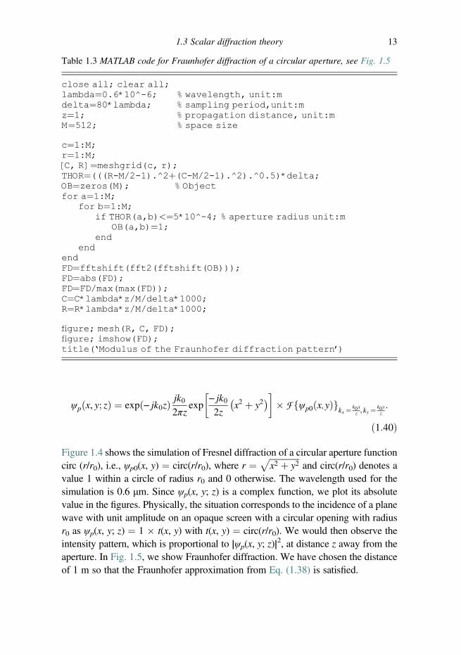
Figure 1.5 (a) Three-dimensional plot of a Fraunhofer diffraction pattern atz ¼ 1 m, |ψp(x, y; z ¼ 1 m)|. (b) Gray-scale plot of |ψp(x, y; z ¼ 1 m)|. See Table1.3 for the MATLAB code.


The term π[(x0)2 þ (y0)2]max is like the maximum area of the source and if this areadivided by the wavelength is much less than the distance z under consideration, theterm exp{(− jk0/2z)[(x0)

2 þ (y0)2]} inside the integrand can be considered to beunity, and hence Eq. (1.36) becomes


− jk02z

ðx2 þ y2Þ

�ðð∞−∞

ψp0ðx0, y0Þexpjk0zðxx0 þ yy0Þ

dx0 dy0: ð1:39Þ

Equation (1.39) is the Fraunhofer diffraction formula and is the limiting case ofFresnel diffraction. Equation (1.39) is therefore called the Fraunhofer approximationor the far field approximation as diffraction is observed at a far distance. In terms ofFourier transform, we can write the Fraunhofer diffraction formula as follows:

Table 1.2 MATLAB code for Fresnel diffraction of a circular aperture, see Fig. 1.4

close all; clear all;lambda¼0.6*10^-6; % wavelength, unit:mdelta¼10*lambda; % sampling period,unit:mz¼0.07; % propagation distance; mM¼512; % space size

c¼1:M;r¼1:M;[C, R]¼ meshgrid(c, r);THOR¼((R-M/2-1).^2þ(C-M/2-1).^2).^0.5;RR¼THOR.*delta;OB¼zeros(M); % Objectfor a¼1:M;

for b¼1:M;if RR(a,b)<¼5*10^-4; % aperture radius unit:m

OB(a,b)¼1;end

endend

QP¼exp(1i*pi/lambda/z.*(RR.^2));FD¼fftshift(fft2(fftshift(OB.*QP)));FD¼abs(FD);FD¼FD/max(max(FD));figure; imshow(OB);title(‘Circular aperture’)figure; imshow(FD);title(‘Modulus of the Fresnel diffraction pattern’)

12 Wave optics


− jk02z

�x2 þ y2

� � F fψp0ðx,yÞgkx ¼ k0x

z ,ky ¼k0yz:

ð1:40Þ

Figure 1.4 shows the simulation of Fresnel diffraction of a circular aperture functioncirc (r/r0), i.e., ψp0(x, y) ¼ circ(r/r0), where r ¼

ffiffiffiffiffiffiffiffiffiffiffiffiffiffix2 þ y2

pand circ(r/r0) denotes a

value 1 within a circle of radius r0 and 0 otherwise. The wavelength used for thesimulation is 0.6 μm. Since ψp(x, y; z) is a complex function, we plot its absolutevalue in the figures. Physically, the situation corresponds to the incidence of a planewave with unit amplitude on an opaque screen with a circular opening with radiusr0 as ψp(x, y; z) ¼ 1 � t(x, y) with t(x, y) ¼ circ(r/r0). We would then observe theintensity pattern, which is proportional to |ψp(x, y; z)|2, at distance z away from theaperture. In Fig. 1.5, we show Fraunhofer diffraction. We have chosen the distanceof 1 m so that the Fraunhofer approximation from Eq. (1.38) is satisfied.

Table 1.3 MATLAB code for Fraunhofer diffraction of a circular aperture, see Fig. 1.5

close all; clear all;lambda¼0.6*10^-6; % wavelength, unit:mdelta¼80*lambda; % sampling period,unit:mz¼1; % propagation distance, unit:mM¼512; % space size

c¼1:M;r¼1:M;[C, R]¼meshgrid(c, r);THOR¼(((R-M/2-1).^2þ(C-M/2-1).^2).^0.5)*delta;OB¼zeros(M); % Objectfor a¼1:M;

for b¼1:M;if THOR(a,b)<¼5*10^-4; % aperture radius unit:m

OB(a,b)¼1;end

endendFD¼fftshift(fft2(fftshift(OB)));FD¼abs(FD);FD¼FD/max(max(FD));C¼C*lambda*z/M/delta*1000;R¼R*lambda*z/M/delta*1000;

figure; mesh(R, C, FD);figure; imshow(FD);title(‘Modulus of the Fraunhofer diffraction pattern’)


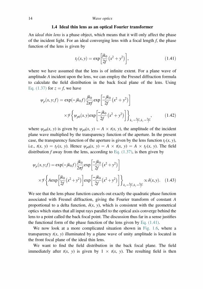
1.4 Ideal thin lens as an optical Fourier transformer

An ideal thin lens is a phase object, which means that it will only affect the phaseof the incident light. For an ideal converging lens with a focal length f, the phasefunction of the lens is given by

tf ðx, yÞ ¼ expjk02f

�x2 þ y2

� , ð1:41Þ

where we have assumed that the lens is of infinite extent. For a plane wave ofamplitude A incident upon the lens, we can employ the Fresnel diffraction formulato calculate the field distribution in the back focal plane of the lens. UsingEq. (1.37) for z ¼ f, we have

ψpðx, y; f Þ ¼ expð− jk0 f Þ jk02πfexp

− jk02f

�x2 þ y2

�

�F ψp0ðx,yÞexp− jk02f

�x2 þ y2

� � �kx ¼ k0x

f ,ky ¼k0yf

, ð1:42Þ

where ψp0(x, y) is given by ψp0(x, y) ¼ A � t(x, y), the amplitude of the incidentplane wave multiplied by the transparency function of the aperture. In the presentcase, the transparency function of the aperture is given by the lens function tf (x, y),i.e., t(x, y) ¼ tf (x, y). Hence ψp0(x, y) ¼ A � t(x, y) ¼ A � tf (x, y). The fielddistribution f away from the lens, according to Eq. (1.37), is then given by

ψpðx,y; f Þ ¼ expð− jk0 f Þ jk02πfexp

− jk02f

�x2þ y2

�

�F Aexpjk02f

�x2þ y2

� exp

− jk02f

�x2þ y2

� � �kx¼ k0x

f ,ky¼k0yf

/ δðx,yÞ: ð1:43Þ

We see that the lens phase function cancels out exactly the quadratic phase functionassociated with Fresnel diffraction, giving the Fourier transform of constant Aproportional to a delta function, δ(x, y), which is consistent with the geometricaloptics which states that all input rays parallel to the optical axis converge behind thelens to a point called the back focal point. The discussion thus far in a sense justifiesthe functional form of the phase function of the lens given by Eq. (1.41).

We now look at a more complicated situation shown in Fig. 1.6, where atransparency t(x, y) illuminated by a plane wave of unity amplitude is located inthe front focal plane of the ideal thin lens.

We want to find the field distribution in the back focal plane. The fieldimmediately after t(x, y) is given by 1 � t(x, y). The resulting field is then

14 Wave optics

undergoing Fresnel diffraction of a distance f. According to Fresnel diffraction andhence using Eq. (1.35), the diffracted field immediately in front of the lens is givenby t(x, y)* h(x, y; f). The field after the lens is then [t(x, y)* h(x, y; f)] � tf(x, y).Finally, the field at the back focal plane is found using Fresnel diffraction one moretime for a distance of f, as illustrated in Fig. 1.6. The resulting field on the backfocal plane of the lens can be written in terms of a series of convolution andmultiplication operations as follows [2]:

ψpðx, yÞ ¼ f½tðx, yÞ � hðx, y; f Þ�tf ðx, yÞg � hðx, y; f Þ: ð1:44Þ

The above equation can be rearranged to become, apart from some constant,

ψpðx, yÞ ¼ F ftðx,yÞgkx ¼ k0x

f ,ky ¼k0yf¼ T

k0x

f,k0y

f

� �, ð1:45Þ

where T(k0x/f, k0y/f ) is the Fourier transform or the spectrum of t(x, y). We see thatwe have the exact Fourier transform of the “input,” t(x, y), on the back focal planeof the lens. Hence an ideal thin lens is an optical Fourier transformer.

1.5 Optical image processing

Figure 1.6 is the backbone of an optical image processing system. Figure 1.7shows a standard image processing system with Fig. 1.6 as the front end of thesystem. The system is known as the 4- f system as lens L1 and lens L2 both have thesame focal length, f. p(x, y) is called the pupil function of the optical system and itis on the confocal plane.

On the object plane, we have an input of the form of a transparency, t(x, y),which is assumed to be illuminated by a plane wave. Hence, according toEq. (1.45), we have its spectrum on the back focal plane of lens L1, T(k0x/f, k0y/f ),where T is the Fourier transform of t(x, y). Hence the confocal plane of the opticalsystem is often called the Fourier plane. The spectrum of the input image is nowmodified by the pupil function as the field immediately after the pupil function

Figure 1.6 Lens as an optical Fourier transformer.

1.5 Optical image processing 15

is T(k0x/f, k0y/f )p(x, y). According Eq. (1.45) again, this field will be Fouriertransformed to give the field on the image plane as

ψpi ¼ F Tk0x

f,k0y

f

� �pðx,yÞ

� �kx ¼ k0x

f ,ky ¼k0yf

, ð1:46Þ

which can be evaluated, in terms of convolution, to give

ψpiðx, yÞ ¼ tð−x, −yÞ � F fpðx, yÞgkx ¼ k0x

f , ky ¼ k0yf

¼ tð−x,−yÞ � P�k0x

f,k0y

f

�¼ tð−x, −yÞ � hcðx, yÞ, ð1:47Þ

where the negative sign in the argument of t(x, y) shows that the original input onthe image plane has been flipped and inverted on the image plane. P is the Fouriertransform of p. From Eq. (1.47), we define hc(x, y) as the coherent point spreadfunction (CPSF) in optics, which is given by [1]

hcðx, yÞ ¼ F fpðx,yÞgkx ¼ k0x

f ,ky ¼k0yf¼ P

k0x

f,k0y

f

� �: ð1:48Þ

By definition, the Fourier transform of the coherent point spread function is thecoherent transfer function (CTF) given by [1]

Hc kx, ky� � ¼ F hc x, yð Þf g ¼ F P

k0x

f,k0y

f

� �� ¼ p

− f kxk0

,− f kyk0

� �: ð1:49Þ

The expression given by Eq. (1.47) can be interpreted as the flipped and invertedimage of t(x, y) being processed by the coherent point spread function given byEq. (1.48). Therefore, image processing capabilities can be varied by simplydesigning the pupil function, p(x, y). Or we can interpret this in the spatialfrequency domain as spatial filtering is proportional to the functional form of the

Figure 1.7 4-f image processing system.

16 Wave optics

pupil function as evidenced by Eq. (1.46) together with Eq. (1.49). Indeed,Eq. (1.46) is the backbone of so-called coherent image processing in optics [1].

Let us look at an example. If we take p(x, y) ¼ 1, this means that we do notmodify the spectrum of the input image according to Eq. (1.46). Or fromEq. (1.49), the coherent transfer function becomes unity, i.e., all-pass filtering,for all spatial frequencies of the input image. Mathematically, using Eq. (1.48) anditem number 8 of Table 1.1, hc(x, y) becomes

hcðx, yÞ ¼ F f1gkx ¼ k0x

f ,ky ¼k0yf¼ 4πδ

k0x

f,k0y

f

� �¼ 4π

f

k0

� �2

δðx, yÞ,

a delta function, and the output image from Eq. (1.47) is

ψpiðx, yÞ / tð−x,−yÞ � δ k0x

f,k0y

f

� �/ tð−x,−yÞ: ð1:50Þ

To obtain the last step of the result in Eq. (1.50), we have used the properties ofδ(x, y) in Table 1.4.

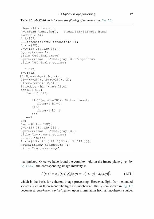
If we now take p(x, y) ¼ circ(r/r0), from the interpretation of Eq. (1.49) we seethat, for this kind of chosen pupil, filtering is of lowpass characteristic as theopening of the circle on the pupil plane only allows the low spatial frequencies tophysically go through. Figure 1.8 shows examples of lowpass filtering. In Fig. 1.8(a) and 1.8(b), we show the original of the image and its spectrum, respectively. InFig. 1.8(c) and 1.8(e) we show the filtered images, and lowpass filtered spectra areshown in Fig. 1.8(d) and 1.8(f), respectively, where the lowpass filtered spectra areobtained by multiplying the original spectrum by circ(r/r0) [see Eq. (1.46)]. Note thatthe radius r0 in Fig. 1.8(d) is larger than that in Fig. 1.8(f). In Fig. 1.9, we showhighpass filtering examples where we take p(x, y) ¼ 1 − circ(r/r0).

So far, we have discussed the use of coherent light, such as plane waves derivedfrom a laser, to illuminate t(x, y) in the optical system shown in Fig. 1.7. Theoptical system is called a coherent optical system in that complex quantities are

Table 1.4 Properties of a delta function

Unit area propertyðð∞−∞

δ x−x0, y−y0Þdx dy ¼ 1ð

Scaling property δðax, byÞ ¼ 1jabj δðx, yÞ

Product property f(x, y) δ(x − x0, y − y0) ¼ f(x0, y0)δ(x − x0, y − y0)

Sampling propertyðð∞−∞

f ðx, yÞδðx−x0, y−y0Þdx dy ¼ f ðx0, y0Þ


Figure 1.8 Lowpass filtering examples: (a) original image, (b) spectrum of (a);(c) and (e) lowpass images; (d) and (f) spectra of (c) and (e), respectively. SeeTable 1.5 for the MATLAB code.

Figure 1.9 Highpass filtering examples: (a) original image, (b) spectrum of (a);(c) and (e) highpass images; (d) and (f) spectra of (c) and (e), respectively. SeeTable 1.6 for the MATLAB code.

18 Wave optics

manipulated. Once we have found the complex field on the image plane given byEq. (1.47), the corresponding image intensity is

Iiðx, yÞ ¼ ψpiðx, yÞψ�piðx, yÞ ¼ jtð−x,−yÞ � hcðx,yÞj2, ð1:51Þ

which is the basis for coherent image processing. However, light from extendedsources, such as fluorescent tube lights, is incoherent. The system shown in Fig. 1.7becomes an incoherent optical system upon illumination from an incoherent source.

Table 1.5 MATLAB code for lowpass filtering of an image, see Fig. 1.8

clear all;close all;A¼imread(‘lena.jpg’); % read 512�512 8bit imageA¼double(A);A¼A/255;SP¼fftshift(fft2(fftshift(A)));D¼abs(SP);D¼D(129:384,129:384);figure;imshow(A);title(‘Original image’)figure;imshow(30.*mat2gray(D)); % spectrumtitle(‘Original spectrum’)

c¼1:512;r¼1:512;[C, R]¼meshgrid(c, r);CI¼((R-257).^2þ(C-257).^2);filter¼zeros(512,512);% produce a high-pass filterfor a¼1:512;

for b¼1:512;

if CI(a,b)>¼20^2; %filter diameterfilter(a,b)¼0;

elsefilter(a,b)¼1;

endend

endG¼abs(filter.*SP);G¼G(129:384,129:384);figure;imshow(30.*mat2gray(G));title(‘Low-pass spectrum’)SPF¼SP.*filter;E¼abs(fftshift(ifft2(fftshift(SPF))));figure;imshow(mat2gray(E));title(‘Low-pass image’)


The optical system manipulates intensity quantities directly. To find the imageintensity, we perform convolution with the given intensity quantities as follows:

Iiðx, yÞ ¼ jtð−x,−yÞj2 � jhcðx,yÞj2: ð1:52ÞEquation (1.52) is the basis for incoherent image processing [1], and |hc(x, y)|

2 isthe intensity point spread function (IPSF) [1]. Note that the IPSF is real and non-negative, which means that it is not possible to implement even the simplestenhancement and restoration algorithms (e.g., highpass, derivatives, etc.), which

Table 1.6 MATLAB code for highpass filtering of an image, see Fig. 1.9


c¼1:512;r¼1:512;[C, R]¼meshgrid(c, r);CI¼((R-257).^2þ(C-257).^2);filter¼zeros(512,512);% produce a high-pass filterfor a¼1:512;

for b¼1:512;

if CI(a,b)<¼20^2; %filter diameterfilter(a,b)¼0;

elsefilter(a,b)¼1;

endend

endG¼abs(filter.*SP);G¼G(129:384,129:384);figure;imshow(2.*mat2gray(G));title(‘High-pass spectrum’)SPF¼SP.*filter;E¼abs(fftshift(ifft2(fftshift(SPF))));figure;imshow(mat2gray(E));title(‘High-pass image’)

20 Wave optics

require a bipolar point spread function. Novel incoherent image processing tech-niques seek to realize bipolar point spread functions (see, for example, [3–6]).

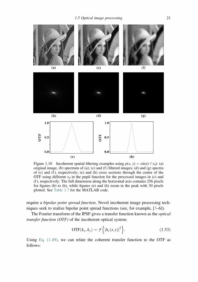
The Fourier transform of the IPSF gives a transfer function known as the opticaltransfer function (OTF) of the incoherent optical system:

OTFðkx, kyÞ ¼ F jhcðx,yÞj2n o

: ð1:53Þ

Using Eq. (1.49), we can relate the coherent transfer function to the OTF asfollows:

Figure 1.10 Incoherent spatial filtering examples using p(x, y) ¼ circ(r / r0): (a)original image, (b) spectrum of (a); (c) and (f ) filtered images; (d) and (g) spectraof (c) and (f ), respectively; (e) and (h) cross sections through the center of theOTF using different r0 in the pupil function for the processed images in (c) and(f ), respectively. The full dimension along the horizontal axis contains 256 pixelsfor figures (b) to (h), while figures (e) and (h) zoom in the peak with 30 pixelsplotted. See Table 1.7 for the MATLAB code.


OTFðkx, kyÞ ¼ Hcðkx, kyÞ � Hcðkx, kyÞ

¼ðð∞−∞

H�cðk0x, k0yÞHcðk0x þ kx, k

0y þ kyÞdk0x dk0y, ð1:54Þ

where � defines correlation [see Table 1.1]. The modulus of the OTF is called themodulation transfer function (MTF), and it is important to note that

jOTFðkx, kyÞj � jOTFð0, 0Þj, ð1:55Þ

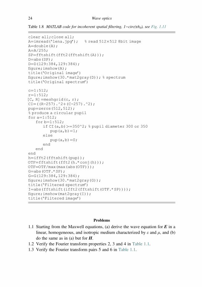
Figure 1.11 Incoherent spatial filtering examples using p(x, y) ¼ 1 − circ(r / r0):(a) original image, (b) spectrum of (a); (c) and (f) filtered images; (d) and (g)spectra of (c) and (f ), respectively; (e) and (h) cross sections through the center ofthe OTF using different r0 in the pupil function for the processed images of (c)and (f), respectively. The full dimension along x contains 256 pixels for figures(b) to (h). See Table 1.8 for the MATLAB code.

22 Wave optics

which states that the MTF always has a central maximum. This signifies that wealways have lowpass filtering characteristics regardless of the pupil function usedin an incoherent optical system. In Figs. 1.10 and 1.11, we show incoherent spatialfiltering results in an incoherent optical system [1] using p(x, y) ¼ circ(r/r0) andp(x, y) ¼ 1 − circ(r/r0), respectively.

Table 1.7 MATLAB code for incoherent spatial filtering, circ(r/r0), see Fig. 1.10


c¼1:512;r¼1:512;[C, R]¼meshgrid(c, r);CI¼((R-257).^2þ(C-257).^2);pup¼zeros(512,512);% produce a circular pupilfor a¼1:512;

for b¼1:512;if CI(a,b)>¼30^2; %pupil diameter 30 or 15

pup(a,b)¼0;else

pup(a,b)¼1;end

endendh¼ifft2(fftshift(pup));OTF¼fftshift(fft2(h.*conj(h)));OTF¼OTF/max(max(abs(OTF)));G¼abs(OTF.*SP);G¼G(129:384,129:384);figure;imshow(30.*mat2gray(G));title(‘Filtered spectrum’)I¼abs(fftshift(ifft2(fftshift(OTF.*SP))));figure;imshow(mat2gray(I));title(‘Filtered image’)


Problems

1.1 Starting from the Maxwell equations, (a) derive the wave equation for E in alinear, homogeneous, and isotropic medium characterized by ε and μ, and (b)do the same as in (a) but for H.

1.2 Verify the Fourier transform properties 2, 3 and 4 in Table 1.1.1.3 Verify the Fourier transform pairs 5 and 6 in Table 1.1.

Table 1.8 MATLAB code for incoherent spatial filtering, 1−circ(r/r0), see Fig. 1.11


c¼1:512;r¼1:512;[C, R]¼meshgrid(c, r);CI¼((R-257).^2þ(C-257).^2);pup¼zeros(512,512);% produce a circular pupilfor a¼1:512;

for b¼1:512;if CI(a,b)>¼350^2; % pupil diameter 300 or 350

pup(a,b)¼1;else

pup(a,b)¼0;end

endendh¼ifft2(fftshift(pup));OTF¼fftshift(fft2(h.*conj(h)));OTF¼OTF/max(max(abs(OTF)));G¼abs(OTF.*SP);G¼G(129:384,129:384);figure;imshow(30.*mat2gray(G));title(‘Filtered spectrum’)I¼abs(fftshift(ifft2(fftshift(OTF.*SP))));figure;imshow(mat2gray(I));title(‘Filtered image’)

24 Wave optics

1.4 Verify the Fourier transform pairs 7, 8, 9, 10, and 11 in Table 1.1.1.5 Assume that the solution to the three-dimensional wave equation in Eq. (1.11)

is given by ψ(x, y, z, t) ¼ ψp(x, y; z)exp( jω0t), verify that the Helmholtzequation for ψp(x, y; z) is given by

∂2ψp

∂x2þ ∂2ψp

∂y2þ ∂2ψp

∂z2þ k20ψp ¼ 0,

where k0 ¼ ω0/ν.1.6 Write down functions of the following physical quantities in Cartesian coord-

inates (x, y, z).(a) A plane wave on the x–z plane in free space. The angle between thepropagation vector and the z-axis is θ.(b) A diverging spherical wave emitted from a point source at (x0, y0, z0) underparaxial approximation.

1.7 A rectangular aperture described by the transparency function t(x, y) ¼rect(x/x0, y / y0) is illuminated by a plane wave of unit amplitude. Determinethe complex field, ψp(x, y; z), under Fraunhofer diffraction. Plot the intensity,|ψp(x, y; z)|

2, along the x-axis and label all essential points along the axis.1.8 Repeat P7 but with the transparency function given by

tðx, yÞ ¼ rectx−X=2

x0,y

y0

� �þ rect

xþ X=2x0

,y

y0

� �, X � x0:

1.9 Assume that the pupil function in the 4-f image processing system in Fig. 1.7is given by rect(x/x0, y / y0). (a) Find the coherent transfer function, (b) give anexpression for the optical transfer function and express it in terms of thecoherent transfer function, and (c) plot both of the transfer functions.

1.10 Repeat P9 but with the pupil function given by the transparency function inP8.

1.11 Consider a grating with transparency function t x, yð Þ ¼ 12 þ 1

2 cos ð2πx=ΛÞ,where Λ is the period of the grating. Determine the complex field, ψp(x, y; z),under Fresnel diffraction if the grating is normally illuminated by a unitamplitude plane wave.

1.12 Consider the grating given in P11. Determine the complex field, ψp(x, y; z),under Fraunhofer diffraction if the grating is normally illuminated by a unitamplitude plane wave.

1.13 Consider the grating given in P11 as the input pattern in the 4-f imageprocessing system in Fig. 1.7. Assuming coherent illumination, find theintensity distribution at the output plane when a small opaque stop is locatedat the center of the Fourier plane.

Problems 25

References

1. T.-C. Poon, and P. P. Banerjee, Contemporary Optical Image Processing withMATLAB (Elsevier, Oxford, UK, 2001).

2. T.-C. Poon, and T. Kim, Engineering Optics with MATLAB (World Scientific, RiverHackensack, NJ, 2006).

3. A. W. Lohmann, and W. T. Rhodes, Two-pupil synthesis of optical transfer functions,Applied Optics 17, 1141–1151 (1978).

4. W. Stoner, Incoherent optical processing via spatially offset pupil masks, AppliedOptics 17, 2454–2467 (1978).

5. T.-C. Poon, and A. Korpel, Optical transfer function of an acousto-optic heterodyningimage processor, Optics Letters 4, 317–319 (1979).

6. G. Indebetouw, and T.-C. Poon, Novel approaches of incoherent image processing withemphasis on scanning methods, Optical Engineering 31, 2159–2167 (1992).

26 Wave optics

2

Fundamentals of holography

2.1 Photography and holography

When an object is illuminated, we see the object as light is scattered to create anobject wave reaching our eyes. The object wave is characterized by two quantities:the amplitude, which corresponds to brightness or intensity, and the phase, whichcorresponds to the shape of the object. The amplitude and phase are convenientlyrepresented by the so-called complex amplitude introduced in Chapter 1. Thecomplex amplitude contains complete information about the object. When theobject wave illuminates a recording medium such as a photographic film or aCCD camera, what is recorded is the variation in light intensity at the plane of therecording medium as these recording media respond only to light intensity.Mathematically, the intensity, I(x, y), is proportional to the complex amplitudesquared, i.e., I(x, y) / |ψp(x, y)|2, where ψp is the two-dimensional complexamplitude on the recording medium. The result of the variation in light intensityis a photograph and if we want to make a transparency from it, the amplitudetransmittance t(x, y) of the transparency can be made proportional to the recordedintensity, or we simply write as follows:

tðx, yÞ ¼ jψpðx,yÞj2: ð2:1Þ

Hence in photography, as a result of this intensity recording, all information aboutthe relative phases of the light waves from the original three-dimensional sceneis lost. This loss of the phase information of the light field in fact destroys thethree-dimensional character of the scene, i.e., we cannot change the perspective ofthe image in the photograph by viewing it from a different angle (i.e., parallax) andwe cannot interpret the depth of the original three-dimensional scene. In essence, aphotograph is a two-dimensional recording of a three-dimensional scene.

Holography is a method invented by Gabor in 1948 [1] in which not only theamplitude but also the phase of the light field can be recorded. The word

27

“holography” combines parts of two Greek words: holos, meaning “complete,” andgraphein, meaning “to write or to record.” Thus, holography means the recordingof complete information. Hence, in the holographic process, the recording mediumrecords the original complex amplitude, i.e., both the amplitude and phase of thecomplex amplitude of the object wave. The result of the recorded intensityvariations is now called a hologram. When a hologram is properly illuminated ata later time, our eyes observe the intensity generated by the same complex field. Aslong as the exact complex field is restored, we can observe the original complexfield at a later time. The restored complex field preserves the entire parallax anddepth information much like the original complex field and is interpreted by ourbrain as the same three-dimensional object.

2.2 Hologram as a collection of Fresnel zone plates

The principle of holography can be explained by recording a point object since anyobject can be considered as a collection of points. Figure 2.1 shows a collimatedlaser split into two plane waves and recombined through the use of two mirrors(M1 and M2) and two beam splitters (BS1 and BS2).

One plane wave is used to illuminate the pinhole aperture (our point object), andthe other illuminates the recording medium directly. The plane wave that is

Figure 2.1 Holographic recording of a point object (realized by a pinhole aperture).

28 Fundamentals of holography

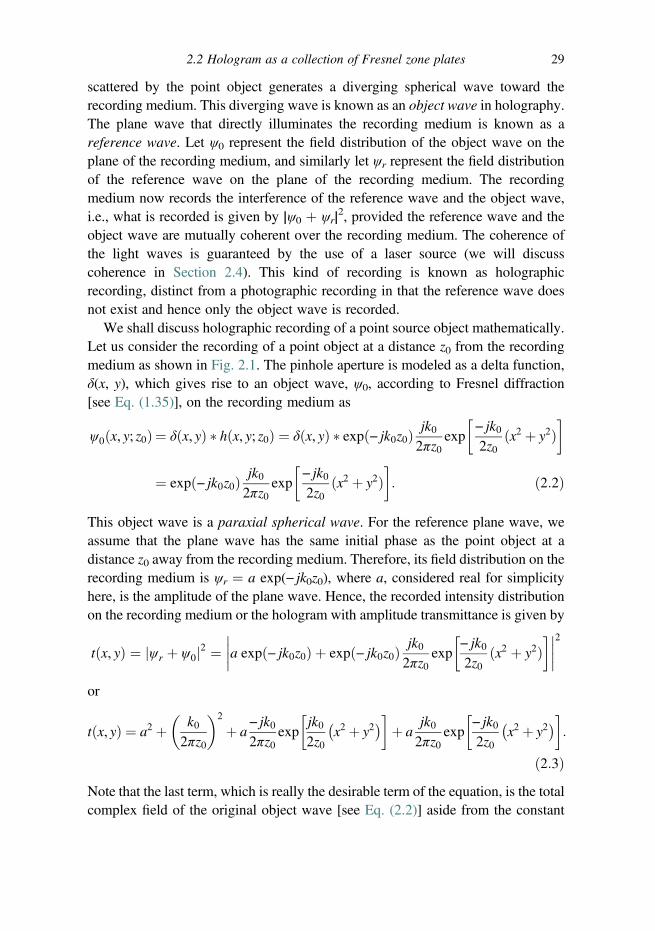
scattered by the point object generates a diverging spherical wave toward therecording medium. This diverging wave is known as an object wave in holography.The plane wave that directly illuminates the recording medium is known as areference wave. Let ψ0 represent the field distribution of the object wave on theplane of the recording medium, and similarly let ψr represent the field distributionof the reference wave on the plane of the recording medium. The recordingmedium now records the interference of the reference wave and the object wave,i.e., what is recorded is given by |ψ0 þ ψr|2, provided the reference wave and theobject wave are mutually coherent over the recording medium. The coherence ofthe light waves is guaranteed by the use of a laser source (we will discusscoherence in Section 2.4). This kind of recording is known as holographicrecording, distinct from a photographic recording in that the reference wave doesnot exist and hence only the object wave is recorded.

We shall discuss holographic recording of a point source object mathematically.Let us consider the recording of a point object at a distance z0 from the recordingmedium as shown in Fig. 2.1. The pinhole aperture is modeled as a delta function,δ(x, y), which gives rise to an object wave, ψ0, according to Fresnel diffraction[see Eq. (1.35)], on the recording medium as

ψ0ðx, y; z0Þ ¼ δðx, yÞ � hðx, y; z0Þ ¼ δðx, yÞ � expð− jk0z0Þ jk02πz0

exp

�− jk02z0

ðx2 þ y2Þ�

¼ expð− jk0z0Þ jk02πz0

exp

�− jk02z0

ðx2 þ y2Þ�: ð2:2Þ

This object wave is a paraxial spherical wave. For the reference plane wave, weassume that the plane wave has the same initial phase as the point object at adistance z0 away from the recording medium. Therefore, its field distribution on therecording medium is ψr ¼ a exp(− jk0z0), where a, considered real for simplicityhere, is the amplitude of the plane wave. Hence, the recorded intensity distributionon the recording medium or the hologram with amplitude transmittance is given by

tðx, yÞ ¼ jψr þ ψ0j2 ¼��a expð− jk0z0Þ þ expð− jk0z0Þ jk0

2πz0exp

− jk02z0

ðx2 þ y2Þ� ��

2

or

t x, yð Þ ¼ a2 þ k02πz0

� �2

þ a− jk02πz0

expjk02z0

x2 þ y2� ��

þ ajk02πz0

exp− jk02z0

x2 þ y2� ��

:

ð2:3ÞNote that the last term, which is really the desirable term of the equation, is the totalcomplex field of the original object wave [see Eq. (2.2)] aside from the constant

2.2 Hologram as a collection of Fresnel zone plates 29

terms a and exp(− jk0z0). Now, Eq. (2.3) can be simplified to a real function and wehave a real hologram given by

tðx, yÞ ¼ Aþ B sink02z0

ðx2 þ y2Þ� �

, ð2:4Þ

where A ¼ a2 þ (k0/2πz0)2 is some constant bias, and B ¼ ak0/πz0. The expressionin Eq. (2.4) is often called the sinusoidal Fresnel zone plate (FZP), which is thehologram of the point source object at a distance z ¼ z0 away from the recordingmedium. Plots of the FZPs are shown in Fig. 2.2, where we have set k0 to be someconstant but for z ¼ z0 and z ¼ 2z0.

When we investigate the quadratic spatial dependence of the FZP, we notice thatthe spatial rate of change of the phase of the FZP, say along the x-direction, isgiven by

f local ¼12π

d

dx

k02z0

x2� �

¼ k0x

2πz0: ð2:5Þ

This is a local fringe frequency that increases linearly with the spatial coordinate, x. Inother words, the further we are away from the center of the zone, the higher the localspatial frequency, which is obvious from Fig. 2.2. Note also from the figure, when wedouble the z value, say from z ¼ z0 to z¼ 2z0, the local fringes become less dense asevident from Eq. (2.5) as well. Hence the local frequency carries the information on z,i.e., from the local frequency we can deduce how far the object point source is awayfrom the recording medium – an important aspect of holography.

To reconstruct the original light field from the hologram, t(x, y), we can simplyilluminate the hologram with plane wave ψrec, called the reconstruction wave in

Figure 2.2 Plots of Fresnel zone plates for z ¼ z0 and z ¼ 2z0.


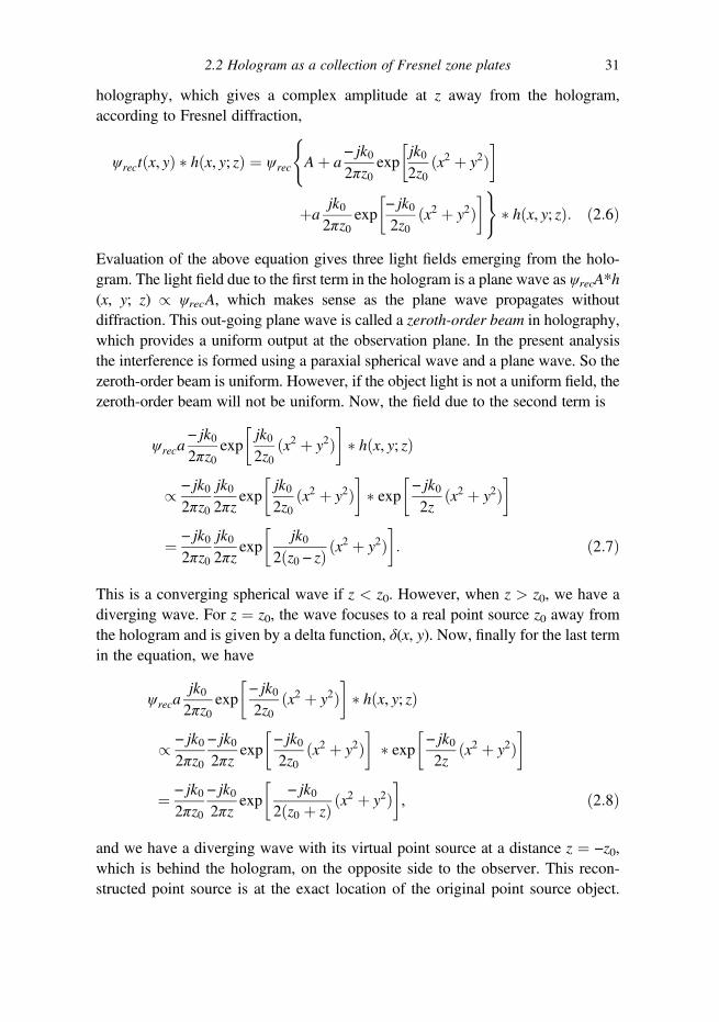
holography, which gives a complex amplitude at z away from the hologram,according to Fresnel diffraction,

ψrectðx, yÞ � hðx, y; zÞ ¼ ψrec

(Aþ a

− jk02πz0

expjk02z0

ðx2 þ y2Þ� �

þajk02πz0

exp− jk02z0

ðx2 þ y2Þ� �)

� hðx, y; zÞ: ð2:6Þ

Evaluation of the above equation gives three light fields emerging from the holo-gram. The light field due to the first term in the hologram is a plane wave as ψrecA*h(x, y; z) / ψrecA, which makes sense as the plane wave propagates withoutdiffraction. This out-going plane wave is called a zeroth-order beam in holography,which provides a uniform output at the observation plane. In the present analysisthe interference is formed using a paraxial spherical wave and a plane wave. So thezeroth-order beam is uniform. However, if the object light is not a uniform field, thezeroth-order beam will not be uniform. Now, the field due to the second term is

ψreca− jk02πz0

exp

�jk02z0

ðx2 þ y2Þ�� hðx, y; zÞ

/ − jk02πz0

jk02πz

exp

�jk02z0

ðx2 þ y2Þ�� exp

�− jk02z

ðx2 þ y2Þ�

¼ − jk02πz0

jk02πz

exp

�jk0

2ðz0 − zÞ ðx2 þ y2Þ

�: ð2:7Þ

This is a converging spherical wave if z < z0. However, when z > z0, we have adiverging wave. For z ¼ z0, the wave focuses to a real point source z0 away fromthe hologram and is given by a delta function, δ(x, y). Now, finally for the last termin the equation, we have

ψrecajk02πz0

exp

�− jk02z0

ðx2 þ y2Þ�� hðx, y; zÞ

/ − jk02πz0

− jk02πz

exp

�− jk02z0

ðx2 þ y2Þ�� exp

�− jk02z

ðx2 þ y2Þ�

¼ − jk02πz0

− jk02πz

exp

�− jk0

2ðz0 þ zÞ ðx2 þ y2Þ

�, ð2:8Þ

and we have a diverging wave with its virtual point source at a distance z ¼ −z0,which is behind the hologram, on the opposite side to the observer. This recon-structed point source is at the exact location of the original point source object.

2.2 Hologram as a collection of Fresnel zone plates 31

The situation is illustrated in Fig. 2.3. The reconstructed real point source is calledthe twin image of the virtual point source.

Although both the virtual image and the real image exhibit the depth of theobject, the virtual image is usually used for applications of three-dimensionaldisplay. For the virtual image, the observer will see a reconstructed image withthe same perspective as the original object. For the real image, the reconstructedimage is a mirror and inside-out image of the original object, as shown in Fig. 2.4.This type of image is called the pseudoscopic image, while the image with normalperspective is called the orthoscopic image. Because the pseudoscopic imagecannot provide natural parallax to the observer, it is not suitable for three-dimensional display.

Let us now see what happens if we have two point source objects given byδ(x, y) þ δ(x − x1, y − y1). They are located z0 away from the recording medium.The object wave now becomes

ψ0ðx, y; z0Þ ¼ ½b0δðx, yÞ þ b1δðx− x1, y− y1Þ� � hðx, y; z0Þ, ð2:9Þwhere b0 and b1 denote the amplitudes of the two point sources. The hologram nowbecomes

reconstruction waveFZP

observer

real imagevirtual image

Figure 2.3 Reconstruction of a FZP with the existence of the twin image (whichis the real image reconstructed in the figure).

Figure 2.4 Orthoscopic and pseudoscopic images.


tðx, yÞ ¼ jψr þ ψ0ðx, y; z0Þj2

¼ a expð− jk0z0Þ þ b0 expð− jk0z0Þ jk02πz0

exp− jk02z0

ðx2 þ y2Þ� ��

þ b1 expð− jk0z0Þ jk02πz0

exp

− jk02z0

ðx− x1Þ2 þ ðy− y1Þ2h i��

2

: ð2:10Þ

Again, the above expression can be put in a real form, i.e., we have

tðx, yÞ ¼ Cþ ab0k0πz0

sin

�k02z0

ðx2 þ y2Þ�þ ab1k0

πz0sin

k02z0

½ðx− x1Þ2 þ ðy− y1Þ2�

þ 2b0b1

�k02πz0

�2

cos

k02z0

½ðx21 þ y21Þ þ 2xx1 þ 2yy1�, ð2:11Þ

where C is again some constant bias obtained similarly as in Eq. (2.4). Werecognize that the second and third terms are our familiar FZP associated to eachpoint source, while the last term is a cosinusoidal fringe grating which comesabout due to interference among the spherical waves. Again, only one term fromeach of the sinusoidal FZPs contains the desirable information as each containsthe original light field for the two points. The other terms in the FZPs areundesirable upon reconstruction, and give rise to twin images. The cosinusoidalgrating in general introduces noise on the reconstruction plane. If we assume thetwo point objects are close together, then the spherical waves reaching therecording medium will intersect at small angles, giving rise to interference fringesof low spatial frequency. This low frequency as it appears on the recordingmedium corresponds to a coarse grating, which diffracts the light by a smallangle, giving the zeroth-order beam some structure physically. Parker Givens haspreviously given a general form of such a hologram due to a number of pointsources [2, 3].

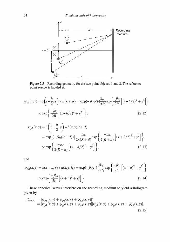
2.3 Three-dimensional holographic imaging

In this section, we study the lateral and longitudinal magnifications in holographicimaging. To make the situation a bit more general, instead of using plane waves forrecording and reconstruction as in the previous section, we use point sources. Weconsider the geometry for recording shown in Fig. 2.5. The two point objects,labeled 1 and 2, and the reference wave, labeled R, emit spherical waves that, onthe plane of the recording medium, contribute to complex fields, ψp1, ψp2, and ψpR,respectively, given by

2.3 Three-dimensional holographic imaging 33

ψp1ðx, yÞ ¼ δ

�x−

h

2, y

�� hðx, y;RÞ ¼ expð− jk0RÞ jk0

2πRexp

− jk02R

hðx−h=2Þ2 þ y2

i

/ exp

− jk02R

hðx−h=2Þ2 þ y2

i, ð2:12Þ

ψp2ðx, yÞ ¼ δ

�xþ h

2, y

�� hðx, y;Rþ dÞ

¼ exp�ð− jk0ðRþ dÞÞ� jk0

2πðRþ dÞ exp

− jk02ðRþ dÞ ðxþ h=2Þ2 þ y2

h i

/ exp

− jk0

2ðRþ dÞ ðxþ h=2Þ2 þ y2h i

, ð2:13Þ

and

ψpRðx, yÞ ¼ δðxþ a, yÞ � hðx, y; l1Þ ¼ expð− jk0l1Þ jk02πl1

exp

− jk02l1

ðxþ aÞ2 þ y2h i

/ exp

− jk02l1

ðxþ aÞ2 þ y2h i

: ð2:14Þ

These spherical waves interfere on the recording medium to yield a hologramgiven by

tðx, yÞ ¼ jψp1ðx, yÞ þ ψp2ðx, yÞ þ ψpRðx, yÞj2¼ ½ψp1ðx, yÞ þ ψp2ðx, yÞ þ ψpRðx, yÞ�½ψ�

p1ðx, yÞ þ ψ�p2ðx, yÞ þ ψ�

pRðx, yÞ�,ð2:15Þ

Figure 2.5 Recording geometry for the two point objects, 1 and 2. The referencepoint source is labeled R.


where the superscript * represents the operation of a complex conjugate. Ratherthan write down the complete expression for t(x, y) explicitly, we will, on the basisof our previous experience, pick out some relevant terms responsible for imagereconstruction. The terms of relevance are treli(x, y), where i ¼ 1,2,3,4

trel1ðx, yÞ ¼ ψ�p1ðx, yÞψpRðx, yÞ

¼ exp

jk02R

½ðx−h=2Þ2 þ y2�� exp

− jk02l1

½ðxþ aÞ2 þ y2�, ð2:16aÞ

trel2ðx, yÞ ¼ ψ�p2ðx, yÞψpRðx, yÞ

¼ exp

jk0

2ðRþ dÞ ½ðxþ h=2Þ2 þ y2�� exp

− jk02l1

½ðxþ aÞ2 þ y2�,

ð2:16bÞ

trel3ðx, yÞ ¼ ψp1

�x, yÞψ�

pR x, yÞ ¼ ½trel1 x,yÞ��,ðð ð2:16cÞtrel4ðx, yÞ ¼ ψp2

�x, yÞψ�

pR x, yÞ ¼ ½trel2 x,yÞ��:ðð ð2:16dÞNote that trel3(x, y) and trel4(x, y) contain the original wavefronts ψp1(x, y) andψp2(x, y) of points 1 and 2, respectively, and upon reconstruction they give rise tovirtual images as shown in the last section for a single point object. However,trel1(x, y) and trel2(x, y) contain the complex conjugates of the original complexamplitudes ψ�

p1 x, yð Þ and ψ�p2 x, yð Þ of points 1 and 2, respectively, and upon

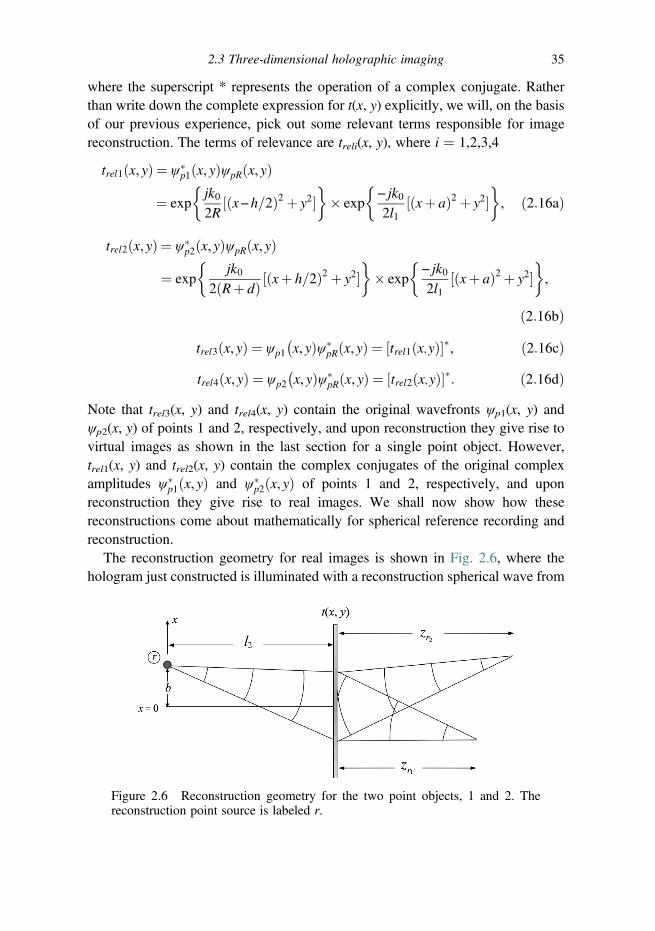
reconstruction they give rise to real images. We shall now show how thesereconstructions come about mathematically for spherical reference recording andreconstruction.

The reconstruction geometry for real images is shown in Fig. 2.6, where thehologram just constructed is illuminated with a reconstruction spherical wave from

Figure 2.6 Reconstruction geometry for the two point objects, 1 and 2. Thereconstruction point source is labeled r.


a point source labeled r. For simplicity, we assume that the wavelength of thereconstruction wave is the same as that of the waves of the recording process.

Hence the complex field, ψpr (x, y), illuminating the hologram is

ψprðx, yÞ¼ δðx− b, yÞ � hðx, y; l2Þ ¼ expð− jk0l2Þ jk02πl2

exp

− jk02l2

ðx− bÞ2 þ y2h i

/ exp

− jk02l2

ðx− bÞ2 þ y2h i

: ð2:17Þ

We find the total complex field immediately behind (away from the source) thehologram by multiplying Eq. (2.17) with Eq. (2.15) but the reconstructions due tothe relevant terms are

ψpr x, yÞtreli x, yÞ,ðð ð2:18Þwhere the treli are defined in Eqs. (2.16).

Consider, first, the contribution from ψpr (x, y)trel1 (x, y). After propagationthrough a distance z behind the hologram, the complex field is transformedaccording to the Fresnel diffraction formula. Note that because the field is conver-ging, it will contribute to a real image. Explicitly, the field can be written as

ψprðx, yÞtrel1ðx, yÞ � hðx, y; zÞ

¼ ψprðx, yÞtrel1ðx, yÞ � expð− jk0zÞjk02πz

exp

�− jk02z

ðx2 þ y2Þ�

/ exp

− jk02l2

½ðx− bÞ2 þ y2�exp

jk02R

½ðx− h=2Þ2 þ y2�

exp

− jk02l1

½ðxþ aÞ2 þ y2�� jk02πz

exp

�− jk02z

ðx2 þ y2Þ�: ð2:19Þ

From the definition of convolution integral [see Table 1.1], we perform theintegration by writing the functions involved with new independent variablesx0, y0 and (x − x0, y − y0). We can then equate the coefficients of x02, y02, appearingin the exponents, to zero, thus leaving only linear terms in x0, y0. Doing this forEq. (2.19), we have

1R−1l1−1l2−

1zr1

¼ 0, ð2:20Þ

where we have replaced z by zr1. zr1 is the distance of the real image reconstructionof point object 1 behind the hologram. We can solve for zr1 to get

zr1 ¼ 1R−1l1−1l2

� �−1¼ Rl1l2

l1l2 − ðl1 þ l2ÞR : ð2:21Þ


At this distance, we can write Eq. (2.19) as

ψprðx, yÞtrel1ðx, yÞ � hðx, y; zr1Þ

/ðð∞−∞

exp

�jk0

�−

h

2R−a

l1þ b

l2þ x

zr1

�x0 þ jk0

y

zr1y0�dx0dy0

/ δ

�xþ zr1

�b

l2−

h

2R−a

l1

�, y

�, ð2:22Þ

which is a δ function shifted in the lateral direction and is a real image of pointobject 1. The image is located zr1 away from the hologram and at

x ¼ x1 ¼ −zr1b

l2−

h

2R−a

l1

� �, y ¼ y1 ¼ 0:

As for the reconstruction due to the relevant term ψpr (x, y)trel2 (x, y) in thehologram, we have

ψprðx, yÞtrel2ðx, yÞ � hðx, y; zÞ

¼ ψprðx, yÞtrel2ðx, yÞ � expð− jk0zÞjk02πz

exp

�− jk02z

x2 þ y2� ��

/ exp

− jk02l2

ðx−bÞ2 þ y2h i

exp

jk0

2ðRþ dÞ xþ h=2ð Þ2 þ y2h i

exp

− jk02l1

ðxþ aÞ2 þ y2h i

� jk02πz

exp

�− jk02z

x2 þ y2� ��

: ð2:23Þ

A similar analysis reveals that this is also responsible for a real image reconstruc-tion but for point object 2, expressible as

ψprðx, yÞtrel2ðx, yÞ � hðx, y; zr2Þ / δ xþ zr2b

l2þ h

2ðRþ dÞ−a

l1

� �, y

� �, ð2:24Þ

where

zr2 ¼ 1Rþ d

−1l1−1l2

� �−1¼ ðRþ dÞl1l2

l1l2−ðl1 þ l2ÞðRþ dÞ :

Here, zr2 is the distance of the real image reconstruction of point object 2 behindthe hologram and the image point is located at

x ¼ x2 ¼ −zr2b

l2þ h

2ðRþ dÞ−a

l1

� �, y ¼ y2 ¼ 0:


Equation (2.24) could be obtained alternatively by comparing Eq. (2.23) with(2.19) and noting that we only need to change R to R þ d and h to −h. The realimage reconstructions of point objects 1 and 2 are shown in Fig. 2.6. The locationsof the virtual images of point objects 1 and 2 can be similarly calculated startingfrom Eqs. (2.16c) and (2.16d).

2.3.1 Holographic magnifications

We are now in a position to evaluate the lateral and longitudinal magnifications ofthe holographic image and this is best done with the point images we discussed inthe last section. The longitudinal distance (along z) between the two real pointimages is zr2 − zr1, so the longitudinal magnification is defined as

MrLong ¼

zr2 − zr1d

: ð2:25Þ

Using Eqs. (2.21) and (2.24) and assuming R � d, the longitudinal magnificationbecomes

MrLong ffi

ðl1l2Þ2ðl1l2 −Rl1 −Rl2Þ2

: ð2:26Þ

We find the lateral distance (along x) between the two image points 1 and 2 bytaking the difference between the locations of the two δ-functions in Eqs. (2.22)and (2.24), so the lateral magnification is

MrLat ¼

zr2

�b

l2þ h

2ðRþ dÞ−a

l1

�− zr1

�b

l2−

h

2R−a

l1

�

h

ffizr2 − zr1ð Þ

�b

l2−a

l1

�þ zr2 þ zr1ð Þ h

2R

hð2:27Þ

for R � d. In order to make this magnification independent of the lateral separ-ation between the objects, h, we set

b

l2−a

l1¼ 0,

or

b

l2¼ a

l1: ð2:28Þ


Then, from Eq. (2.27) and again for the condition that R � d,

MrLat ’ zr2 þ zr1ð Þ 1

2R’ l1l2

l1l2 − ðl1 þ l2ÞR : ð2:29Þ

By comparing Eq. (2.26) and Eq. (2.29), we have the following important rela-tionship between the magnifications in three-dimensional imaging:

MrLong ¼ ðMr

LatÞ2: ð2:30Þ

2.3.2 Translational distortion

In the above analysis of magnifications, we have assumed that the condition ofEq. (2.28) is satisfied in the reconstruction. If Eq. (2.28) is violated, the lateralmagnification will depend on the lateral separation between the object points. Inother words, the reconstructed image will experience translational distortion. Tosee clearly the effect of translational distortion, let us consider point objects 1 and 2along the z-axis by taking h ¼ 0 and inspecting their image reconstitution loca-tions. The situation is shown in Fig. 2.7. Points 1 and 2 are shown in the figure as areference to show the original image locations. Points 10 and 20 are reconstructedreal image points of object points 1 and 2, respectively, due to the reconstructionwave from point r. We notice there is a translation between the two real imagepoints along the x-direction. The translational distance Δx is given by

Δx ¼ x1 − x2,

where x1 and x2 are the locations previously found [see below Eqs. (2.22) and(2.24)]. For h ¼ 0, we find the translational distance

Δx ¼ ðzr2 − zr1Þ b

l2−a

l1

� �: ð2:31Þ

Figure 2.7 Translational distortion of the reconstructed real image.


From the above result, we see that the image is twisted for a three-dimensionalobject. In practice we can remove the translational distortion by setting the recon-struction point to satisfy Eq. (2.28). The distortion can also be removed by settinga ¼ b ¼ 0. However, by doing so, we lose the separation of the real, virtual, andzeroth-order diffraction, a situation reminiscent of what we observed in Fig. 2.3where we used plane waves for recording and reconstruction, with both the planewaves traveling along the same direction. We will discuss this aspect more inChapter 3.

Example 2.1: Holographic magnification

In this example, we show that by using a spherical wave for recording and planewave reconstruction, we can produce a simple magnification imaging system. Westart with a general result for Mr

Lat given by Eq. (2.27):

MrLat ¼

zr2b

l2þ h

2ðRþ dÞ−a

l1

� �− zr1

b

l2−

h

2R−a

l1

� �h

: ð2:32Þ

For a¼ b¼ 0, i.e., the recording and reconstruction point sources are on the z-axis,and d ¼ 0, i.e., we are considering a planar image, Mr

Lat becomes

MrLat ¼

zr2 þ zr12R

¼ 1−R

l1−R

l2

� �−1, ð2:33Þ

where zr2 ¼ zr1 ¼ [1/R − 1/l1 − 1/l2]−1. For plane wave reconstruction, l2 ! ∞.Equation (2.33) finally becomes a simple expression given by

MrLat ¼ 1−

R

l1

� �−1: ð2:34Þ

For example, taking l1 ¼ 2R, MrLat ¼ 2, a magnification of a factor of 2, and for

l1 ¼ 1/4R < R, MrLat ¼ −1=3, a demagnification in this case. Note that if the

recording reference beam is also a plane wave, i.e., l1 ! ∞, there is no magnifica-tion using a plane wave for recording and reconstruction.

2.3.3 Chromatic aberration

In the above discussion, the wavelength of the reconstruction wave was assumed tobe the same as that of the wave used for holographic recording. If the hologram isilluminated using a reconstruction wave with a different wavelength, λr, then thesituation becomes much more complicated. Now the reconstruction wave canstill be found using Eq. (2.19) but ψpr (x, y) and h(x, y; z) must be modifiedaccording to


ψprðx, yÞ / exp− jkr2l1

ðx− aÞ2 þ y2

�� ,

and

hðx, y; zÞ / jkr2πz

exp− jkr2z

ðx2 þ y2Þ� �

,

respectively, where kr ¼ 2π/λr. Hence the longitudinal distance of the real imagereconstruction [see Eq. (2.21)] is modified to become

zr1 ¼ λrλ0R

−λrλ0l1

−1l2

� �−1¼ λ0Rl1l2

λrl1l2 − ðλrl2 þ λ0l1ÞR : ð2:35Þ

Accordingly, the transverse location can be found from Eq. (2.22) to give

x1 ¼ − zr1b

l2−

hλr2Rλ0

−aλrl1λ0

� �, y1 ¼ 0: ð2:36Þ

Thus in general the location of the image point depends on the wavelength of thereconstruction wave, resulting in chromatic aberration. We can see that for R � l1and R � l2,

zr1 � λ0λrR, ð2:37aÞ

x1 � h

2þ R

a

l1−b

l2

λ0λr

� �: ð2:37bÞ

As a result, in chromatic aberration, the shift of the image location due to thedifference of the wavelength used for recording and reconstruction is proportionalto R, the distance of the object from the hologram.

Example 2.2: Chromatic aberration calculation

We calculate the chromatic aberration of an image point in the following case:R ¼ 5 cm, h ¼ 2 cm, a ¼ b ¼ 5 cm, l1 ¼ l2 ¼ 20 cm, λ0 ¼ 632 nm.

We define the longitudinal aberration distance, and the transverse aberrationdistance, δx, as

δz ¼ zr1ðλrÞ− zr1ðλ0Þ, ð2:38aÞδx ¼ x1ðλrÞ− x1ðλ0Þ: ð2:38bÞ

δz and δx are plotted in Fig. 2.8 with the MATLAB code listed in Table 2.1. Incomparison with the desired image point, zr1 (λ0) ¼ 10 cm and x1 (λ0) ¼ 2 cm, theamount of aberration increases as the deviation from the desired wavelength, λ0,becomes larger so that holograms are usually reconstructed with a single


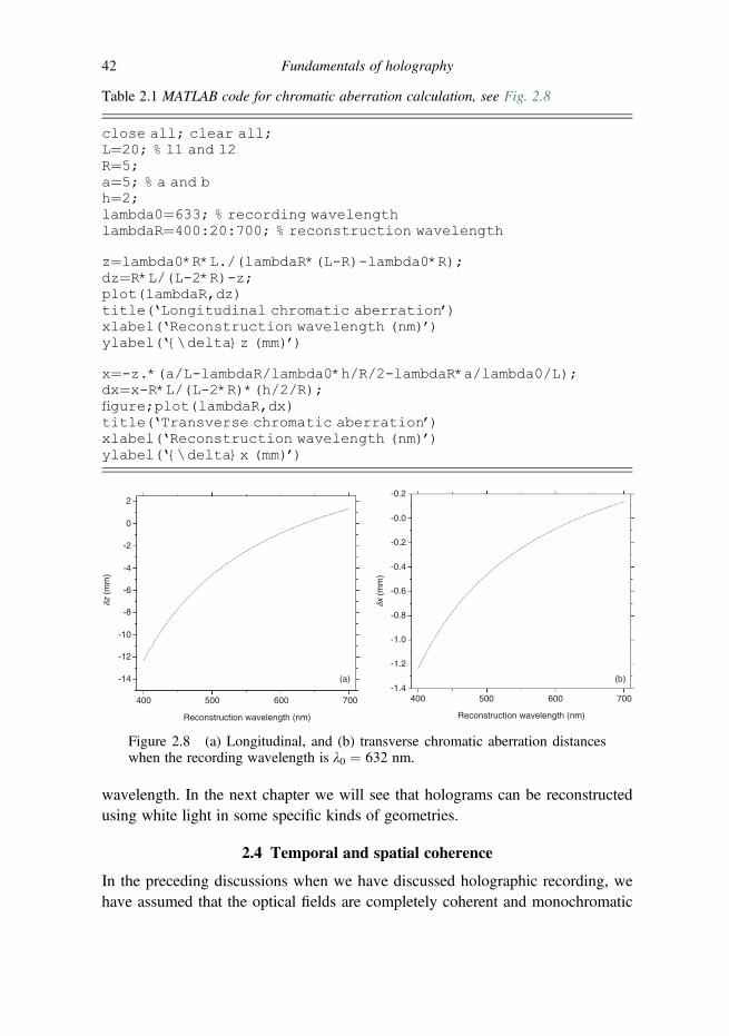
wavelength. In the next chapter we will see that holograms can be reconstructedusing white light in some specific kinds of geometries.

2.4 Temporal and spatial coherence

In the preceding discussions when we have discussed holographic recording, wehave assumed that the optical fields are completely coherent and monochromatic

Table 2.1 MATLAB code for chromatic aberration calculation, see Fig. 2.8

close all; clear all;L¼20; % l1 and l2R¼5;a¼5; % a and bh¼2;lambda0¼633; % recording wavelengthlambdaR¼400:20:700; % reconstruction wavelength

z¼lambda0*R*L./(lambdaR*(L-R)-lambda0*R);dz¼R*L/(L-2*R)-z;plot(lambdaR,dz)title(‘Longitudinal chromatic aberration’)xlabel(‘Reconstruction wavelength (nm)’)ylabel(‘{\delta}z (mm)’)

x¼-z.*(a/L-lambdaR/lambda0*h/R/2-lambdaR*a/lambda0/L);dx¼x-R*L/(L-2*R)*(h/2/R);figure;plot(lambdaR,dx)title(‘Transverse chromatic aberration’)xlabel(‘Reconstruction wavelength (nm)’)ylabel(‘{\delta}x (mm)’)

dz (

mm

)

dx (

mm

)

2

0

-2

-4

-6

-8

-10

-12

-14

-1.2

-1.0

-0.8

-0.6

-0.4

-0.2

-0.0

-0.2

-1.4400 500 600 700 400 500 600 700

Reconstruction wavelength (nm)

(a) (b)

Reconstruction wavelength (nm)

Figure 2.8 (a) Longitudinal, and (b) transverse chromatic aberration distanceswhen the recording wavelength is λ0 ¼ 632 nm.


so that the fields will always produce interference. In this section, we give a briefintroduction to temporal and spatial coherence. In temporal coherence, we areconcerned with the ability of a light field to interfere with a time-delayed version ofitself. In spatial coherence, the ability of a light field to interfere with a spatiallyshifted version of itself is considered.

2.4.1 Temporal coherence

In a simplified analysis of interference, light is considered to be monochromatic,i.e., the bandwidth of the light source is infinitesimal. In practice there is no idealmonochromatic light source. A real light source contains a range of frequenciesand hence interference fringes do not always occur. An interferogram is a photo-graphic record of intensity versus optical path difference of two interfering waves.The interferogram of two light waves at r is expressed as

I¼DjAðr, tÞ þ Bðr, tÞj2

E¼

DjAðr, tÞj2

EþDjBðr, tÞj2

Eþ 2� Re

n�A�ðr, tÞBðr, t��o, ð2:39Þ

where 〈〉 stands for the time-average integral as

hi ¼ limT!∞

1T

ðT=2−T=2

dt, ð2:40Þ

and A(r, t) and B(r, t) denote the optical fields to be superimposed. In the followingdiscussion we will first assume that the two light fields are from an infinitesimal,quasi-monochromatic light source. We model the quasi-monochromatic light ashaving a specific frequency ω0 for a certain time and then we change its phaserandomly. Thus at fixed r, A(t) and B(t) can be simply expressed as

AðtÞ ¼ A0exp�j½ω0t þ θðtÞ��, ð2:41aÞ

BðtÞ ¼ B0exp�j½ω0ðt þ τÞ þ θðt þ τÞ��, ð2:41bÞ

where τ denotes the time delay due to the optical path difference between A(t) andB(t), and θ(t) denotes the time-variant initial phase of the quasi-monochromaticlight. By substituting Eq. (2.41) into Eq. (2.39), we have

IðτÞ ¼ A20 þ B2

0 þ 2A0B0 � Ren�

e j θ tþτð Þ − θ tð Þþω0τ½ ��o ð2:42Þbecause hjA tð Þj2i ¼ A2

0 and hjBðtÞj2i ¼ B20. In Eq. (2.42), the time-average integral

is the interference term called the complex degree of coherence of the source,which is denoted as

2.4 Temporal and spatial coherence 43

γðτÞ ¼De j½θðtþτÞ − θðtÞþω0τ�

E: ð2:43Þ

The complex degree of coherence has the properties

γð0Þ ¼ 1 and jγðτÞj 1: ð2:44ÞAs a result, the interferogram can be expressed in terms of the complex degree ofcoherence as


0 þ 2A0B0jγðτÞj cos ½argfγðτÞg�, ð2:45Þwhere {} stands for the operation of taking the argument of the function beingbracketed. It should be noted that in Eq. (2.45) the modulus of the complex degreeof coherence comes into existence only when we measure the intensity and it is notdirectly obtainable. In fact, the modulus of the complex degree of coherence is easyto determine by measuring the contrast between fringes in I(τ), as first performedby Michelson. The fringe contrast is called the fringe visibility ν, defined by

ν ¼ Imax − IminImax þ Imin

, ð2:46Þ

where Imax and Imin denote the local maximum value and the local minimum valueof the interferogram, respectively. Accordingly, we can see that

Imax¼ A20 þ B2

0 þ 2A0B0jγðτÞj,Imin ¼ A2

0 þ B20 − 2A0B0jγðτÞj:

So the visibility of the interferogram in Eq. (2.46) can be expressed as

ν ¼ 2A0B0

A20 þ B2

0

jγ τð Þj: ð2:47Þ

Equation (2.47) shows that the modulus of the degree of coherence is proportionalto the visibility of the fringe. So we can deduce the ability to form interferencefrom a light source if we know its coherence property. We say that light wavesinvolved in an interferometer are completely coherent, completely incoherent, orpartially coherent according to the value of |γ(τ)|:

jγðτÞj ¼ 1 complete coherencejγðτÞj ¼ 0 complete incoherence

0 jγðτÞj 1 partial coherence:

Let us take a simple plane wave as an example, i.e., A(t) ¼ A0 exp( jω0t), andB(t) ¼ A0 exp[ jω0(t þ τ)]. Equation (2.43) becomes γ(τ) ¼ exp( jω0τ) and therefore

|γ(τ)| ¼ 1, a case of complete coherence. On the other hand, if A(t) is completelyrandom in time, from Eq. (2.43), we have γ(τ) ¼ 0, a case of complete incoherence.


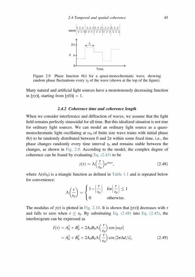
Many natural and artificial light sources have a monotonously decreasing functionin |γ(τ)|, starting from |γ(0)| ¼ 1.

2.4.2 Coherence time and coherence length

When we consider interference and diffraction of waves, we assume that the lightfield remains perfectly sinusoidal for all time. But this idealized situation is not truefor ordinary light sources. We can model an ordinary light source as a quasi-monochromatic light oscillating at ω0 of finite size wave trains with initial phaseθ(t) to be randomly distributed between 0 and 2π within some fixed time, i.e., thephase changes randomly every time interval τ0 and remains stable between thechanges, as shown in Fig. 2.9. According to the model, the complex degree ofcoherence can be found by evaluating Eq. (2.43) to be

γðτÞ ¼ Λ ττ0

�e jω0τ, ð2:48Þ

where Λ(τ/τ0) is a triangle function as defined in Table 1.1 and is repeated belowfor convenience:

Λττ0

� �¼ 1−

�� ττ0

�� for�� ττ0

�� 1

0 otherwise:

8<:

The modulus of γ(τ) is plotted in Fig. 2.10. It is shown that |γ(τ)| decreases with τand falls to zero when τ � τ0. By substituting Eq. (2.48) into Eq. (2.45), theinterferogram can be expressed as


0 þ 2A0B0Λ ττ0

�cos ½ω0τ�

¼ A20 þ B2

0 þ 2A0B0Λ ττ0

�cos ½2πΔd=λ�, ð2:49Þ

wave

t02p

pq

0Time

Figure 2.9 Phase function θ(t) for a quasi-monochromatic wave, showingrandom phase fluctuations every τ0 of the wave (shown at the top of the figure).


where Δd is the optical path difference corresponding to the time delay τ betweenthe two light waves, i.e., 2πΔd/λ ¼ ω0τ.

The width of the complex degree of coherence, τ0, is called the coherence time.If the time delay between the light waves involved in the interference is larger thanthe coherence time, no fringes can be observed.

Finally, we can also define the coherence length lc as

ℓc ¼ cτ0, ð2:50Þwhere c is the speed of light in vacuum. In other words, the coherence length is thepath the light passes in the time interval τ0. To ensure the success of interference,the optical path difference in an interferometer must be smaller than the coherencelength.

2.4.3 Some general temporal coherence considerations

In the above discussion, we used the model of a quasi-monochromatic light so thatthe analysis is relatively simple. Here we will extend the theory to any kind of lightsource. In Eq. (2.42), the complex degree of coherence comes from the process oftime average of the cross term. On the other hand, we also know that γ(0) ¼ 1according to Eq. (2.44). Thus for any light source, we can write down the complexdegree of coherence as:

γðτÞ ¼ hE��tÞEðt þ τÞihjEðtÞj2i , ð2:51Þ

where E(t) is the complex amplitude of the light at the source point. Equation (2.51)is the general form of the complex degree of coherence. It should be noted that thefrequency range of the optical wave E(t) cannot be detected directly using anymodern photodetectors. Hence, to evaluate Eq. (2.51), we first express the timeaverage 〈E* (t)E(t þ τ)〉 as an auto-correlation calculation,

1

0.5

0

� g �

t0

t

Figure 2.10 The modulus of the complex degree of coherence for quasi-monochromatic light.


hE�ðtÞEðt þ τÞi¼ limT!∞

1T

ðT=2−T=2

E�ðtÞEðt þ τÞ dt

/ ½EðτÞ � EðτÞ�: ð2:52ÞFrom the correlation of the Fourier transform in Table 1.1, we have

F τfEðτÞ�EðτÞg ¼ð∞−∞

½EðτÞ�EðτÞ�expð− jωτÞdτ ¼ jF τfEðτÞgj2 ¼ P cðωÞ, ð2:53Þ

where we define the one-dimensional temporal Fourier transform of f(τ) as

F τf f ðτÞg ¼ð∞−∞

f ðτÞexpð− jωτÞdτ ¼ FðωÞ, ð2:54aÞ

and the inverse temporal Fourier transform is

F −1τ fFðωÞg ¼ 1

2π

ð∞−∞

FðωÞexpð jωτÞdω ¼ f ðτÞ, ð2:54bÞ

where τ and ω are the time and the temporal radian frequency variables, respect-ively. Note that the definitions of F τ and F −1

τ are different from those of F and F −1

for the spatial function defined in Eq. (1.22); namely “−j” is used in the exponen-tial function for the time function in the forward transform. This is done purposelyto be consistent with the engineering convention for a traveling wave. In theconvention, exp[j(ω0t − k0z)] denotes a plane wave traveling in the þz-direction.However, we can still use Table 1.1 as long as we replace “j” by “−j” in thetransform pairs.

Let us return our attention to Eq. (2.53). The result of Eq. (2.53) is the Wiener–Khinchin theorem, which states that the Fourier transform of the auto-correlation ofthe light field is proportional to the power spectrum of the light source, P cðωÞ.P cðωÞ is the power spectrum of the complex field E, i.e., a field represented by acomplex quantity. It should be noted that P cðωÞ is not the same as P rðωÞ, thepower spectrum of the real light field where the light field is expressed in terms of areal quality. P rðωÞ includes both þω and −ω components, while P cðωÞ containsonly the þω component. As it turns out, the relation between P cðωÞ and P rðωÞ issimple, namely [4]

P cðωÞ ¼4P rðωÞ for ω > 00 for ω < 0:


As a result, Eq. (2.51) can be re-written to become

γðτÞ ¼ F −1τ fP cðωÞg

F −1τ fP cðωÞgτ¼0

¼ F −1τ fPNðωÞg, ð2:55Þ

where PNðωÞ is the normalized power spectrum of the source and it ensures γ(0)¼ 1.

2.4.4 Fourier transform spectroscopy

In practice, the power spectrum can be deduced from measurements of I(τ). We letA(t) ¼ A0(ω) e

jωt, a plane wave of frequency ω with its amplitude given by A0(ω),and B(t) ¼ A0(ω) e

j(ωt þ τ) as B(t) is the time-delayed version of the same pointfrom the source. According to Eq. (2.39),

IðτÞ ¼ hjA0ðωÞe jωt þ A0ðωÞe jðωtþτÞj2i ¼ 2jA0ðωÞj2½1þ cos ðωτÞ�: ð2:56ÞNow we take the source which is composed of a collection of waves with differentfrequencies as follows:

EðtÞ ¼ð∞0

A0ðωÞexpðjωtÞdω: ð2:57Þ

The total contribution from all the frequencies to I(τ) then becomes

IðτÞ¼ð∞0

2jA0ðωÞj2½1þ cos ðωτÞ�dω

/ 2ð∞0

P rðωÞdω þ 2ð∞0

P rðωÞ cos ðωτÞdω

/ 2 I0 þ ΔIðτÞ: ð2:58ÞAs jA0ðωÞj2 / P rðωÞ, the power spectrum of the source, the first term in the aboveequation is a constant and simply proportional to the total intensity of the lightsource, I0. The second term ΔI(τ) varies with the delay τ. Note that the powerspectrum is only given for positive frequencies and by letting P rð−ωÞ ¼ P rðωÞ, aneven function in ω, we can extend the second term of the equation to become

ΔIðτÞ¼ 2ð∞0

P rðωÞ cos ðωτÞdω ¼ð∞−∞

P rðωÞexpð jωτÞdω

/ 12π

ð∞−∞

P rðωÞexpð jωτÞdω ¼ F −1τ fP rðωÞg: ð2:59Þ


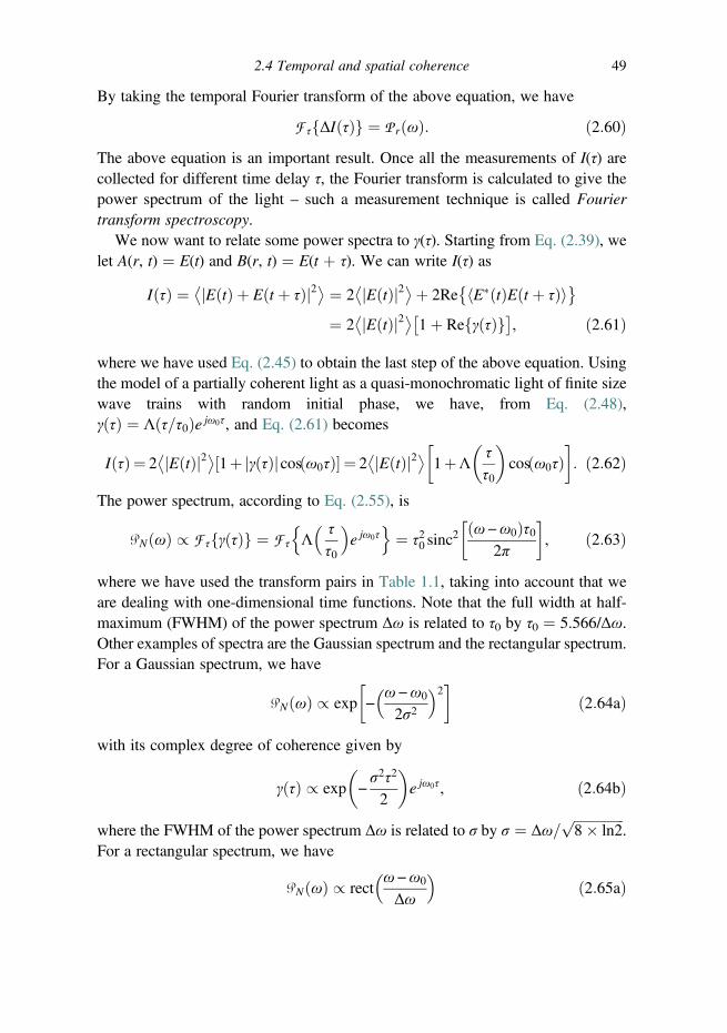
By taking the temporal Fourier transform of the above equation, we have

F τfΔIðτÞg ¼ P rðωÞ: ð2:60ÞThe above equation is an important result. Once all the measurements of I(τ) arecollected for different time delay τ, the Fourier transform is calculated to give thepower spectrum of the light – such a measurement technique is called Fouriertransform spectroscopy.

We now want to relate some power spectra to γ(τ). Starting from Eq. (2.39), welet A(r, t) ¼ E(t) and B(r, t) ¼ E(t þ τ). We can write I(τ) as

IðτÞ ¼ �jEðtÞ þ Eðt þ τÞj2� ¼ 2�jEðtÞj2�þ 2Re

�hE�ðtÞEðt þ τÞi�¼ 2

�jEðtÞj2� 1þ RefγðτÞg�,� ð2:61Þ

where we have used Eq. (2.45) to obtain the last step of the above equation. Usingthe model of a partially coherent light as a quasi-monochromatic light of finite sizewave trains with random initial phase, we have, from Eq. (2.48),γðτÞ ¼ Λðτ=τ0Þe jω0τ, and Eq. (2.61) becomes

IðτÞ ¼ 2�jEðtÞj2�½1þjγðτÞjcosðω0τÞ� ¼ 2

�jEðtÞj2� 1þΛττ0

� �cosðω0τÞ

� �: ð2:62Þ

The power spectrum, according to Eq. (2.55), is

PNðωÞ / F τfγðτÞg ¼ F τ

nΛ ττ0

�e jω0τ

o¼ τ20 sinc

2 ðω−ω0Þτ02π

� �, ð2:63Þ

where we have used the transform pairs in Table 1.1, taking into account that weare dealing with one-dimensional time functions. Note that the full width at half-maximum (FWHM) of the power spectrum Δω is related to τ0 by τ0 ¼ 5.566/Δω.Other examples of spectra are the Gaussian spectrum and the rectangular spectrum.For a Gaussian spectrum, we have

PNðωÞ / exp −ω−ω0

2σ2

�2� �

ð2:64aÞ

with its complex degree of coherence given by

γðτÞ / exp −σ2τ2

2

� �e jω0τ, ð2:64bÞ

where the FWHM of the power spectrum Δω is related to σ by σ ¼ Δω=ffiffiffiffiffiffiffiffiffiffiffiffiffiffiffi8� ln2

p.

For a rectangular spectrum, we have

PNðωÞ / rectω−ω0

Δω

�ð2:65aÞ


and its complex degree of coherence is

γðτÞ / sincΔωτ2π

� �ejω0τ: ð2:65bÞ

Although we have indicated that the coherence time is the width of |γ(τ)|, formost practical light sources it is hard to determine the coherence time byintuition. So here we adopt the definition of coherence time τc proposed byMandel [5], that is

τc ð∞−∞

jγ τð Þj2dτ: ð2:66Þ

For example, the coherence time of a quasi-monochromatic light is found to beτc ¼ 2τ0/3 according to the definition in Eq. (2.66). Finally, the coherence timealways has a value of the same order of magnitude as the reciprocal of thebandwidth of the source, that is

τc � 2πΔω

: ð2:67Þ

As a result, we can also show that, using Eqs. (2.50) and (2.67) and taking τc � τ0,we have

ℓc � λ2

Δλ, ð2:68Þ

where Δλ is the spectral line width of the source and λ is the wavelength corres-ponding to the center frequency of the power spectrum ω0. We can also relate thespectral line width to the FWHM of the power spectrum Δω as follows:

Δω � 2πc

λ2Δλ: ð2:69Þ

White light has a line width of about 300 nm, ranging roughly from 400 to 700 nm,and if we take the average wavelength at 550 nm, Eq. (2.68) gives ℓ�c 1 μm, a veryshort coherence length. LEDs have a spectral width Δλ of about 50 nm and have acoherence length of about 7 μm for red color with wavelength of 0.6 μm. As for thegreen line of mercury at 546 nm having a line width about 0.025 nm, its coherencelength is about 1.2 cm. Lasers typically have a long coherence length. Helium–

neon lasers can produce light with coherence lengths greater than 5 m, but 20 cm istypical. Some industrial CO2 lasers of line width of around 10−5 nm producingemission at the infrared wavelength of 10.6 μm would give a coherence length ofaround 11 km.


2.4.5 Spatial coherence

In the above discussion of temporal coherence, light was assumed to be emittedfrom an infinitesimal source and we have found the ability of two relativelydelayed light waves to form fringes. In practice, any light source must have a sizeof extended area, and light emitted from any two points of this area is incoherent.In this subsection, the dependence of the finite size of the quasi-monochromaticincoherent light source on interference is discussed, which brings us to the conceptof spatial coherence.

To simplify the analysis, we first consider interference including two identicalbut incoherent quasi-monochromatic light sources, as shown in Fig. 2.11. If there isa single point source, say source 1, light emitted from the source is separated intotwo paths, one path passing through point A and the other path through pointB. Light emerging from points A and B comes to the screen to form interferencefringes. Hence we may think of A and B as two slits in this situation. Thecorresponding analysis is similar to that in the above subsection. Now we will dealwith the case that two point sources, source 1 and source 2, exist at the same time.

In the plane of the screen where we have interference, we only consider point P,the center of the screen. Thus the optical path difference between AP and BP iszero. At point P, we have

I¼ �jEAðtÞ þ EBðtÞj2�

¼ �jEAðtÞj2�þ �jEBðtÞj2

�þ 2� Re�hEA

�ðtÞEBðtÞi�, ð2:70Þ

where

EAðtÞ ¼ E1AðtÞ þ E2AðtÞ, ð2:71aÞand

EBðtÞ ¼ E1BðtÞ þ E2BðtÞ ð2:71bÞ

Figure 2.11 Schematic diagram of interference formed by two incoherent lightsources.


are the optical fields passing through point A and point B, respectively; E1i(t) andE2i(t) are the components emitted from source 1 and source 2, respectively, wherethe subscript i ¼ A or B. According to the concept of temporal coherence [Eq.(2.51)], we can define the complex degree of coherence between points A and B,that is

γAB ¼�E�AðtÞEBðtÞ

�ffiffiffiffiffiffiffiffiffiffiffiffiffiffiffiffiffiffiffiffiffiffiffiffiffiffiffiffiffiffiffiffiffiffiffiffiffiffiffi�jEAðtÞj2

��jEBðtÞj2�q , ð2:72Þ

which is called the complex degree of mutual coherence, and γ of Eq. (2.51) is,strictly speaking, the complex degree of self coherence.

Because source 1 and source 2 are completely incoherent, they cannot interferewith each other, i.e., cross terms such as E�

1AðtÞE2BðtÞ ¼ 0, E�2AðtÞE1BðtÞ ¼ 0, etc.

Thus we have the following results:

hE�AðtÞEBðtÞi ¼ hE�

1AðtÞE1BðtÞi þ hE�2AðtÞE2BðtÞi,�jEAj2

�¼ �jE1Aj2�þ �jE2Aj2

�,�jEBj2

�¼ �jE1B

��2i þ �jE2Bj2�:

Suppose that�jE1Aj2

� � �jE1Bj2� � �jE2Aj2

� � h��E2Bj2�for simplicity, then we

can rewrite Eq. (2.72) as

γAB ¼ hE�1AðtÞE1BðtÞi

2h��E1AðtÞj2� þ hE�

2AðtÞE2BðtÞi2�jE2AðtÞj2

� : ð2:73Þ

Because both E1A(t) and E1B(t) come from the same source, their relationship mustbe E1B(t) ¼ E1A(t þ τ1); similarly, we will also have E2B(t) ¼ E2A(t þ τ2), where τ1and τ2 are the time delays between the waves at point A and point B, respectively,from source 1 and source 2. As a result, the complex degree of coherence γAB canbe expressed as

γAB ¼ hE�1AðtÞE1Aðt þ τ1Þi2h��E1AðtÞj2

� þ hE�2AðtÞE2Aðt þ τ2Þi2h��E2AðtÞj2

�¼ 1

2γ1ðτ1Þ þ

12γ2ðτ2Þ: ð2:74Þ

Equation (2.74) shows that γAB depends on the complex degree of coherence of thetwo source points.

If the light emitted from the two point sources is quasi-monochromatic, we canuse the result from Eq. (2.48) for Eq. (2.74) to yield

γAB ¼ 12Λ

τ1τ0

� �e jωτ1 þ 1

2Λ

τ2τ0

� �e jωτ2 : ð2:75Þ


After some manipulation, the modulus of the complex degree of coherence can beexpressed as

jγABj2 �12½1þ cos ωðτ1 − τ2Þ�Λ τ1

τ0

� �Λ

τ2τ0

� �ð2:76Þ

provided that τ1 � τ2 � ðτ1 − τ2Þ. Hence the period of the cosine function inEq. (2.76) is much shorter than that of the triangle function and the cosine functiondominates the visibility of the interferogram. By applying the simple geometrydescribed in Fig. 2.11 and using the paraxial approximation, we can obtain

τ2 − τ1 ¼ sl

rc, ð2:77Þ

where s is the separation of the two light sources, l is the separation of points A andB, and r is the separation of the source plane from the plane of points A andB. Finally, we can say that the interference fringes are visible, provided

ωðτ1 − τ2Þ < π,

or

l <rλ2s

: ð2:78Þ

To understand the meaning of Eq. (2.78), we can imagine that in Fig. 2.11 pointA is a movable pinhole while point B is a fixed pinhole. When the separationbetween point A and point B is very short, i.e., l � rλ=2s, the visibility of theinterferogram on the screen approaches unity. When the separation between pointA and point B is rλ=2s, the visibility falls to zero. As a result, we can define thetransverse coherence length lt as

lt ¼ rλ2s

¼ λ2θs

, ð2:79Þ

where θs ¼ s/r is the angular separation of the source measured from the plane ofpoints A and B. In other words, we can improve the spatial coherence by movingthe source far away from the plane of points A and B.

2.4.6 Some general spatial coherence considerations

In the above discussion, the quasi-monochromatic incoherent light source onlyincludes two points. This is, of course, not the real situation. In practice, the sourceis extended and consists of numerous independent point sources. Now we want toknow the correlation between a fixed point B and another fixed point A. As shownin Fig. 2.12(a), every point source S in the source emits light to both point A and


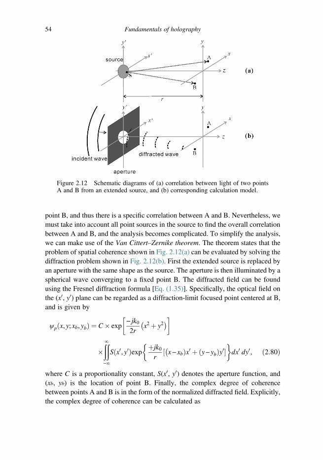
point B, and thus there is a specific correlation between A and B. Nevertheless, wemust take into account all point sources in the source to find the overall correlationbetween A and B, and the analysis becomes complicated. To simplify the analysis,we can make use of the Van Cittert–Zernike theorem. The theorem states that theproblem of spatial coherence shown in Fig. 2.12(a) can be evaluated by solving thediffraction problem shown in Fig. 2.12(b). First the extended source is replaced byan aperture with the same shape as the source. The aperture is then illuminated by aspherical wave converging to a fixed point B. The diffracted field can be foundusing the Fresnel diffraction formula [Eq. (1.35)]. Specifically, the optical field onthe (x0, y0) plane can be regarded as a diffraction-limit focused point centered at B,and is given by

ψpðx, y; xb, ybÞ ¼ C� exp

�− jk02r

x2 þ y2� ��

�ðð∞−∞

S x0, y0ð Þexpþjk0

r½�x− xbÞx0 þ ðy− ybÞy0�

dx0 dy0, ð2:80Þ

where C is a proportionality constant, S(x0, y0) denotes the aperture function, and(xb, yb) is the location of point B. Finally, the complex degree of coherencebetween points A and B is in the form of the normalized diffracted field. Explicitly,the complex degree of coherence can be calculated as

Figure 2.12 Schematic diagrams of (a) correlation between light of two pointsA and B from an extended source, and (b) corresponding calculation model.


γAB ¼

ðð ∞

−∞Sðx0, y0Þexp

þjk0r ½ðxa − xbÞx0 þ ðya − ybÞy0�

dx0 dy0ðð ∞

−∞Sðx0, y0Þdx0 dy0

¼F fSðx,yÞg

kx¼k0ðxa − xbÞr ,ky¼k0ðya − ybÞ

rðð ∞

−∞Sðx0, y0Þdx0 dy0

, ð2:81Þ

where (xa, ya) is the location of point A.

Example 2.3: Double-pinhole interference

Consider a double-pinhole interference experiment. The geometry is shown inFig. 2.13. Two pinholes A and B are located at xa ¼ 1 mm, ya ¼ 0 and xb ¼ −1 mm,yb ¼ 0, respectively. The light source is a lamp of extended size with a goodbandpass filter centered at 600 nm. We can improve the spatial coherence by placinga small circular aperture against the light source. The distance between the apertureand the two pinholes is r ¼ 20 cm. We shall calculate the largest available aperturediameter so that the visibility of the resulting interference fringe is larger than 0.5.

The light source with the circular aperture is given by S(x, y) ¼ circ(r/r0), wherer ¼

ffiffiffiffiffiffiffiffiffiffiffiffiffiffix2 þ y2

p. According to Eq. (2.81), the complex degree of coherence is

calculated as

γAB / Fourier transform of circðr=r0Þ ¼ 2J1ðr0krÞr0kr

, ð2:82Þ

where ðkr ¼ k0=rÞffiffiffiffiffiffiffiffiffiffiffiffiffiffiffiffiffiffiffiffiffiffiffiffiffiffiffiffiffiffiffiffiffiffiffiffiffiffiffiðxa−xbÞ2 þ ðya−ybÞ2

q, and J1() is a Bessel function of the

first kind, order 1. So γAB is a function of r0 and is plotted in Fig. 2.14. Thecorresponding MATLAB code is listed in Table 2.2. It is shown in Fig. 2.14 that r0

Figure 2.13 Double-pinhole experiment to evaluate coherence.


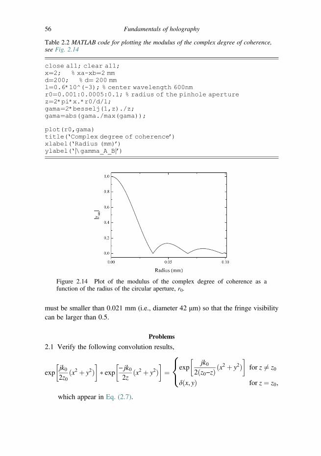
must be smaller than 0.021 mm (i.e., diameter 42 μm) so that the fringe visibilitycan be larger than 0.5.

Problems

2.1 Verify the following convolution results,

expjk02z0

ðx2 þ y2Þ� �

� exp − jk02z

ðx2 þ y2Þ� �

¼

(exp

�jk0

2ðz0−zÞ ðx2 þ y2Þ

�for z 6¼ z0

δðx, yÞ for z ¼ z0,

which appear in Eq. (2.7).

Table 2.2 MATLAB code for plotting the modulus of the complex degree of coherence,see Fig. 2.14

close all; clear all;x¼2; % xa-xb¼2 mmd¼200; % d¼ 200 mml¼0.6*10^(-3); % center wavelength 600nmr0¼0.001:0.0005:0.1; % radius of the pinhole aperturez¼2*pi*x.*r0/d/l;gama¼2*besselj(1,z)./z;gama¼abs(gama./max(gama));

plot(r0,gama)title(‘Complex degree of coherence’)xlabel(‘Radius (mm)’)ylabel(‘j\gamma_A_Bj’)

Figure 2.14 Plot of the modulus of the complex degree of coherence as afunction of the radius of the circular aperture, r0.


2.2 With reference to Fig. 2.5 and Fig. 2.6 for the recording and reconstructiongeometry of point sources, let a ¼ b ¼ 0, i.e., the reference and reconstructionpoint sources are on the z-axis, and show that the lateral magnification for thevirtual image is [6]

MvLat ¼ 1−

R

l1þ R

l2

� �−1,

and the longitudinal magnification for R � d is

MvLong ¼

ðl1l2Þ2ðl1l2 þ Rl1 −Rl2Þ2

:

2.3 Show that for a quasi-monochromatic light oscillating at ω0 of finite size wavetrains with initial phase distributed randomly between 0 and 2π within somefixed time, i.e., the phase randomly changes every time interval τ0 and remainsstable between the changes, as shown in Fig. 2.9, the complex degree ofcoherence is given by

γ τð Þ ¼ Λττ0

� �e jω0τ:

2.4 According to the definition of coherence time given by Mandel, show that thecoherence time of the quasi-monochromatic light from Problem 2.3 is givenby τc ¼ 2τ0/3.

2.5 The typical bandwidth of a commercial He–He laser operated at λ ¼ 632.8 nmis about 500 MHz. Calculate the corresponding coherence length.

2.6 A bandpass filter is usually applied in association with a broadband lightsource to produce interference. Typically, the full width half-maximum(FWHM) of the transmission band is 10 nm while the center wavelength ofthe band is λ ¼ 630 nm. Calculate the corresponding coherence length.

2.7 When we investigate the interference formed by two incoherent light sourcesshown in Fig. 2.11, τ1 and τ2 are the time delays between the waves at point Aand point B, respectively from source 1 and source 2. Show that τ2 − τ1 ¼ sl/rc,assuming the small angle approximation.

2.8 Show that for two point sources that are quasi-monochromatic, the complexdegree of mutual coherence

jγABj2 ¼12Λ

τ1τ0

� �ejωτ1 þ 1

2Λ

τ2τ0

� �e jωτ2

� 12½1þ cos ωðτ1−τ2Þ�Λ τ1

τ0

� �Λ

τ2τ0

� �

if τ1 � τ2 � (τ1 − τ2).

Problems 57

2.9 Start from the Fresnel diffraction formula [Eq. (1.35)] and assume a sphericalwave passing through an aperture S(x, y) converging to (xb, yb) at thediffraction plane [Fig. 2.12(b)]. Find the diffracted field as given by the resultin Eq. (2.80).

2.10 Show that the complex degree of coherence of the light produced by auniformly quasi-monochromatic incoherent source with a shape of circulardisk of radius r0 is proportional to J1()/() given by Eq. (2.82). Note thatsince the problem is of circular symmetry, it is convenient to express theFourier transform as follows.

F f f x, yð Þg ¼ F kx, ky� � ¼ 2π

ð∞0

rf rð ÞJ0 krrð Þdr,

where r ¼ffiffiffiffiffiffiffiffiffiffiffiffiffiffix2 þ y2

p, kr ¼

ffiffiffiffiffiffiffiffiffiffiffiffiffiffiffiffiffiffikx2 þ ky2

p, and J0() is the zeroth-order Bessel

function. The above integral is also referred to as the Fourier–Bessel transformdenoted by

ℬf f rð Þg ¼ 2πð∞0

rf rð ÞJ0 krrð Þdr:

References

1. D. Garbor, A new microscopic principle, Nature 161, 777–778 (1948).2. M. P. Givens, Introduction to holography, American Journal of Physics 35, 1056–1064

(1967).3. T.-C. Poon, On the fundamentals of optical scanning holography, American Journal of

Physics 76, 738–745 (2008).4. J. W. Goodman, Statistical Optics (John Wiley & Sons, New York, 1985).5. L. Mandel, Fluctuations of photon beams: the distribution of the photo-electrons,

Proceedings of the Physical Society 74, 233 (1959).6. F. T. S. Yu, Optical Information Processing (John Wiley & Sons, New York, 1983).


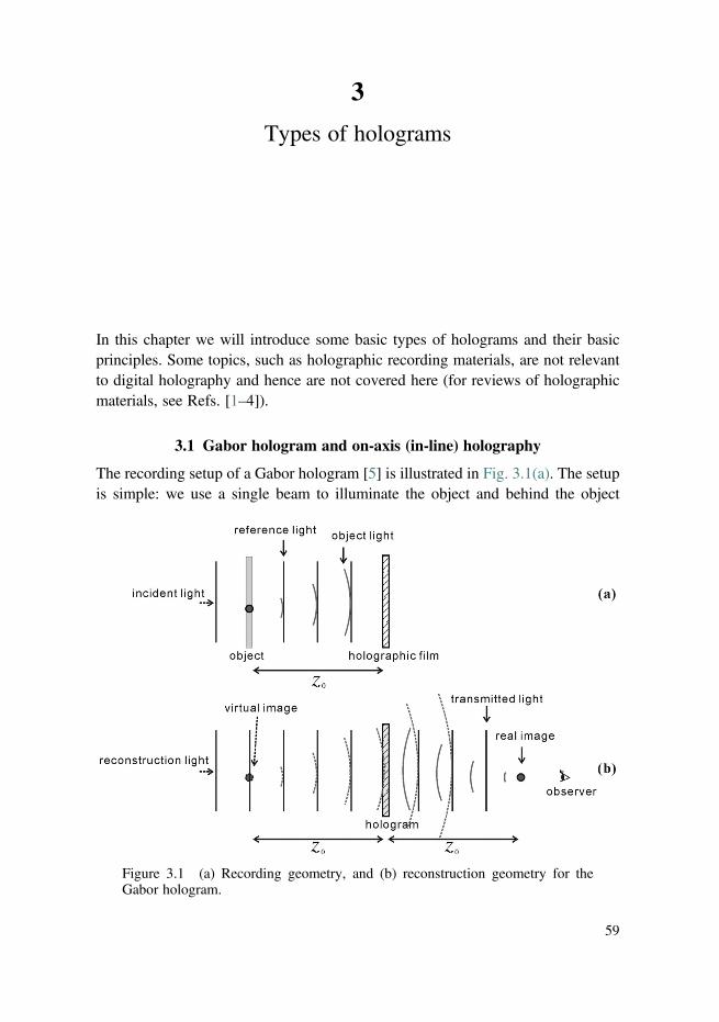
3

Types of holograms

In this chapter we will introduce some basic types of holograms and their basicprinciples. Some topics, such as holographic recording materials, are not relevantto digital holography and hence are not covered here (for reviews of holographicmaterials, see Refs. [1–4]).

3.1 Gabor hologram and on-axis (in-line) holography

The recording setup of a Gabor hologram [5] is illustrated in Fig. 3.1(a). The setupis simple: we use a single beam to illuminate the object and behind the object

Figure 3.1 (a) Recording geometry, and (b) reconstruction geometry for theGabor hologram.

59

a photosensitive material or device is placed as a recording medium. The method iseffective only when the object is limited to a small fluctuation Δ(x, y) of a uniformtransparency σ0 so that the object wave scattered by the object does not disturb theuniform reference wave excessively. Hence the total transparency of the objectσ(x, y) can be expressed as

σðx, yÞ ¼ σ0 þ Δðx, yÞ ð3:1Þwith the condition that Δ(x, y) � σ0. Therefore, the complex field on the hologramplane, at a distance z0 away from the object, can be expressed as

uðx, yÞ ¼ A½σ0 þ Δðx, yÞ� � hðx, y; z0Þ ¼ ψc þ ψ0ðx, yÞ, ð3:2Þwhere A is the amplitude of the incident light, and h(x, y; z0) is the spatial impulseresponse [Eq. (1.34)]. ψc is a uniform transmitting field, which can serve as thereference light and the scattered field, ψ0(x, y), as the amplitude fluctuation isregarded as the object field. As a result, the intensity on the hologram plane or thehologram with amplitude transmittance can be expressed as

tðx, yÞ ¼ jψc þ ψ0 ðx,yÞj2 ¼ jψcj2 þ jψ0ðx,yÞj2 þ ψcψ�0 ðx, yÞ þ ψ�

cψ0ðx, yÞ: ð3:3ÞIn the reconstruction process, the hologram, t(x, y), is illuminated by a plane waveof the reconstruction light. The complex field emerging from the hologram is thenproportional to

jψcj2 þ jψ0ðx,yÞj2 þ ψcψ�0ðx, yÞ þ ψ�

cψ0ðx, yÞ: ð3:4ÞAccording to the analysis in Section 2.2, ψcψ

�0 x, yð Þ reconstructs a real image, i.e.,

a complex conjugate duplicate of the object (the twin image) at a distance z0 behindthe hologram. We can see it clearly as

ψcψ�0ðx, yÞ � hðx, y; z0Þ ¼ ψc½AΔðx,yÞ � hðx,y; z0Þ�� hðx, y; z0Þ / Δ�ðx, yÞ:

Similarly, ψ�cψ0ðx, yÞ reconstructs a virtual image of the amplitude fluctuation

Δ(x, y) at the location of the object. After back-propagating a distance of z0,we have

ψ�cψ0ðx, yÞ � h�ðx, y; z0Þ ¼ ψ�

c ½AΔðx, yÞ � hðx, y; z0Þ� � h�ðx, y; z0Þ / Δðx, yÞ:The first two terms of Eq. (3.4) correspond to the transmitted zeroth-order beamgiven by

jψcj2 þ jψ0ðx,yÞj2h i

� hðx, y; zÞ,

where z is any distance behind the hologram. The reconstruction is shown inFig. 3.1(b).

60 Types of holograms

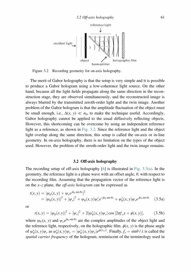
The merit of Gabor holography is that the setup is very simple and it is possibleto produce a Gabor hologram using a low-coherence light source. On the otherhand, because all the light fields propagate along the same direction in the recon-struction stage, they are observed simultaneously, and the reconstructed image isalways blurred by the transmitted zeroth-order light and the twin image. Anotherproblem of the Gabor hologram is that the amplitude fluctuation of the object mustbe small enough, i.e., Δ(x, y) � σ0, to make the technique useful. Accordingly,Gabor holography cannot be applied to the usual diffusively reflecting objects.However, this shortcoming can be overcome by using an independent referencelight as a reference, as shown in Fig. 3.2. Since the reference light and the objectlight overlap along the same direction, this setup is called the on-axis or in-linegeometry. In on-axis holography, there is no limitation on the types of the objectused. However, the problem of the zeroth-order light and the twin image remains.

3.2 Off-axis holography

The recording setup of off-axis holography [6] is illustrated in Fig. 3.3(a). In thegeometry, the reference light is a plane wave with an offset angle, θ, with respect tothe recording film. Assuming that the propagation vector of the reference light ison the x–z plane, the off-axis hologram can be expressed as

tðx, yÞ ¼ jψ0ðx, yÞ þ ψrejk0 sin θxj2

¼ jψ0ðx, yÞj2 þ jψrj2 þ ψ0ðx, yÞψ�r e

−jk0 sin θx þ ψ�0ðx, yÞψre

jk0 sin θx ð3:5aÞor

tðx, yÞ ¼ jψ0ðx,yÞj2 þ jψrj2 þ 2jψ�0ðx, yÞψrj cos 2πf xxþ ϕðx, yÞ½ �, ð3:5bÞ

where ψ0 (x, y) and ψrejk0 sin θx are the complex amplitudes of the object light and

the reference light, respectively, on the holographic film. ϕ(x, y) is the phase angleof ψ�

0ðx, yÞψr as ψ�0 x, yð Þψr ¼ jψ�

0 x, yð Þψrjejϕ x,yð Þ. Finally, fx ¼ sinθ / λ is called thespatial carrier frequency of the hologram, reminiscent of the terminology used in

Figure 3.2 Recording geometry for on-axis holography.

3.2 Off-axis holography 61

communication systems where a carrier wave is used to “carry” the message in thetheory of modulation. Hence the off-axis hologram is also called the carrier-frequency hologram.

In the reconstruction, the hologram is illuminated by the reconstruction lightalong the same direction as the reference light, as shown in Fig. 3.3(b). Assumingthe amplitude of the reconstruction light is the same as that of the reference light,the complex field just behind the hologram can be expressed as

ψrejk0 sin θx � tðx, yÞ ¼ jψrj2ψre

jk0 sin θx þ jψ0ðx, yÞj2ψrejk0 sin θx

þψ0ðx, yÞjψrj2 þ ψ�0ðx, yÞψ2

r ej2k0 sin θx, ð3:6Þ

where we have used Eq. (3.5a) to write the above equation. Similar to Gaborholography, the first two terms on the right hand side of Eq. (3.6) represent thetransmitted light, i.e., the zeroth-order beam. The third term contributes to thevirtual reconstructed image. Finally, the last term contributes to the conjugate realimage. To understand how the virtual image can be viewed without the annoyingdisturbance due to the transmitted light and the twin image, it is convenient toanalyze the situation in the Fourier spectrum domain. In the spectrum domain, thefour terms on the right side of Eq. (3.6) can be respectively calculated by

Figure 3.3 (a) Recording setup, and (b) reconstruction setup for off-axisholography.


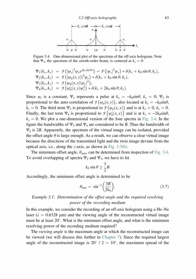
Ψ1ðkx, kyÞ ¼ F fjψrj2ψrejk0 sin θxg ¼ F fjψrj2ψrg � δðkx þ k0 sin θ, kyÞ,

Ψ2ðkx, kyÞ ¼ F fjψ0ðx, yÞj2ψrg � δðkx þ k0 sin θ, kyÞ,Ψ3ðkx, kyÞ ¼ F fψ0ðx, yÞjψrj2g,Ψ4ðkx, kyÞ ¼ F fψ�

0ðx, yÞψ2rg � δðkx þ 2k0 sin θ, kyÞ:

Since ψr is a constant, Ψ1 represents a pulse at kx ¼ −k0sinθ, ky ¼ 0; Ψ2 isproportional to the auto-correlation of F ψ0 x, yð Þf g, also located at kx ¼ −k0sinθ,ky ¼ 0. The third term Ψ3 is proportional to F ψ0 x, yð Þf g and is at kx ¼ 0, ky ¼ 0.Finally, the last term Ψ4 is proportional to F ψ�

0ðx, yÞ� �

and is at kx ¼ −2k0sinθ,ky ¼ 0. We plot a one-dimensional version of the four spectra in Fig. 3.4. In thefigure the bandwidths of Ψ3 and Ψ4 are considered to be B. Thus the bandwidth ofΨ2 is 2B. Apparently, the spectrum of the virtual image can be isolated, providedthe offset angle θ is large enough. As a result, we can observe a clear virtual imagebecause the directions of the transmitted light and the twin image deviate from theoptical axis, i.e., along the z-axis, as shown in Fig. 3.3(b).

The minimum offset angle, θmin, can be determined from inspection of Fig. 3.4.To avoid overlapping of spectra Ψ2 and Ψ3, we have to let

k0 sin θ � 32B

Accordingly, the minimum offset angle is determined to be

θmin ¼ sin−13B2k0

� �: ð3:7Þ

Example 3.1: Determination of the offset angle and the required resolvingpower of the recording medium

In this example, we consider the recording of an off-axis hologram using a He–Nelaser (λ ¼ 0.6328 μm) and the viewing angle of the reconstructed virtual imagemust be at least 20�. What is the minimum offset angle, and what is the minimumresolving power of the recording medium required?

The viewing angle is the maximum angle at which the reconstructed image canbe viewed (we will discuss this further in Chapter 7). Since the required largestangle of the reconstructed image is 20� / 2 ¼ 10�, the maximum spread of the

Figure 3.4 One-dimensional plot of the spectrum of the off-axis hologram. Notethat Ψ3, the spectrum of the zeroth-order beam, is centered at kx ¼ 0.

3.2 Off-axis holography 63

propagation vector along the x-direction is then k0x ¼ k0 � sin (10�). Thus thebandwidth of the reconstructed virtual image is

B ¼ 2� k0 � sin 10�ð Þ ¼ 3448 rad=mm,

where k0 ¼ 2π/0.6328 μm¼ 9929 rad/mm. The factor of two in the above equationcorresponds to taking into account that the spread of the light from the recon-structed image also spills into the negative x-direction. By substituting the calcu-lated value of B into Eq. (3.7), we can determine θmin as

θmin ¼ sin−13� 3448 rad=mm2� 9929 rad=mm

� �¼ 31:4�:

Now, in order to successfully record the off-axis hologram, the recording mediummust be able to resolve the spatial carrier frequency, fx ¼ sinθmin/λ, plus half thebandwidth, B/2, of the reconstructed image, i.e., the required resolvable spatialfrequency is

f resolvable ¼sin θmin

λþ B=2

2π¼ sin θmin

λþ B

4π: ð3:8Þ

With the calculated values of θmin and B, we can find

f resolvable ¼sin 31:4�

632:8 mmþ 3448 rad=mm

2π¼ 1095 cycle=mm or line−pair=mm or lp=mm:

This resolution can be achieved by most available holographic emulsions, typicallyseveral thousand line-pairs per millimeter. However, such resolution is wellbeyond the capability of existing electronic photosensitive devices such as CCDsor spatial light modulators (SLMs). We will discuss SLMs and holographic three-dimensional display in Chapter 7.

3.3 Image hologram

An image hologram can be recorded as shown in Fig. 3.5(a), where a real image ofthe object is formed on the holographic film using a lens. The light emerging fromthe real image serves as the object wave. Mathematically, on recording, the imagehologram is given by

tðx, yÞ ¼ jψiðx,yÞ þ ψr ejk0 sin θxj2, ð3:9Þ

where ψi (x, y) represents the complex field of the real image on the hologram andψr e

jk0 sin θx is the off-axis reference plane wave. Upon reconstruction and assumingthe amplitude of the reconstruction light is the same as that of the reference lightas shown in Fig. 3.5(b), the complexfield just behind the hologram can be expressed as


tðx, yÞ � ψr ejk0 sin θx ¼ ½jψij2 þ jψrj2�e jk0 sin θx þ ψiðx, yÞψ�

r þ ψ�i ðx, yÞψr e

j2k0 sin θx:

ð3:10ÞThe first term of the right hand side of the above equation makes up the zeroth-order beam propagating along the direction of the reconstruction beam. The secondterm is the reconstructed image and is on the hologram plane. The third term is thetwin image, which is reconstructed on the hologram plane as well but propagatingalong the direction that is 2θ away from the z-axis, but the observer views thereconstruction along the z-axis.

We cannot observe the reconstructed image of a conventional off-axis hologramusing a polychromatic light source, such as a lamp, because there is a seriouschromatic aberration in the hologram. As we have shown in Section 2.3.3,chromatic aberration is proportional to the distance between the object and thehologram plane. If the object is reconstructed on the plane of the hologram,chromatic aberration can be minimized and the reconstructed images from variouswavelengths overlap, producing a clear, white reconstructed image. Therefore, theimage hologram can be reconstructed using either monochromatic light or poly-chromatic light. It should be noted that the twin image is also reconstructed on thehologram plane, as shown in Fig. 3.5(b). Thus the off-axis geometry is necessaryfor recording the image hologram and only the reconstructed image can beobserved along the direction of the observer.

Figure 3.5 (a) Recording geometry, and (b) reconstruction geometry for theimage hologram.

3.3 Image hologram 65

Example 3.2: Simulation of an image hologram

In this example, we would like to demonstrate the reconstruction of an imagehologram using white light. To simplify the simulation, we only consider a singlediffraction order (the virtual image) of an off-axis hologram. Thus the off-axiszeroth-order light and the twin image are ignored in the simulation. The objectpattern shown in Fig. 3.6(a) contains 256 � 256 pixels. The pixel pitch is 50 μm,and the recording wavelength is 0.65 μm. The offset angle is 10�. Here we do notdiscuss the details of the discrete Fourier transform and the simulation of diffrac-tion, which will be discussed in Chapter 4.

We first obtain the diffracted field at a desired reconstruction plane using wave-lengths ranging from 0.45 μm to 0.65 μm with wavelength separation of 0.005 μm.Thus we have a total of 41 reconstructed images. We then superimpose the recon-structed images of all the wavelengths, producing a multi-wavelength reconstructedimage. Figure 3.6(b)–(d) are the multi-wavelength reconstructed images while thedistances between the images and the hologram are 1 cm, 5 cm, and 15 cm,respectively. As the distance between the reconstructed image and the hologram isclose (i.e., 1 cm), the hologram can be regarded as an image hologram and we cansee that the reconstructed image is sharp even though the reconstruction light iswhite light. However, as the reconstructed image is far from the hologram plane,

Figure 3.6 Original object (a) and the white-light reconstructed images withdistances between the image and hologram of (b)1 cm, (c) 5 cm, and (d)15 cm,respectively.


Table 3.1 MATLAB code for simulation of an image hologram, see Example 3.2

% Input data, set parametersclear all, close all;Ii¼imread(‘DH256.bmp’);% 256�256 pixels 8bitfigure; imshow(Ii);title(‘Object pattern’)axis off

Ii¼double(Ii);PH¼rand([256,256]);Ii¼Ii.*exp(2i*pi*PH); % add a random phase on the objectM¼512;I¼zeros(512);I(128:383,128:383)¼Ii; % zero padding

z¼15; %(cm, distance) PLEASE CHANGE THE DISTANCE TO 1, 5, 15, ETC.w¼6500*10^-8; %(cm, wavelength)delta¼0.005; % cm, pixel size 50umr¼1:M;c¼1:M;[C, R]¼meshgrid(c, r);

% Forward propagation (650nm)p¼exp(-2i*pi*z.*((1/w)^2-(1/M/delta)^2.*(C-M/2-1).^2-. . .

(1/M/delta)^2.*(R-M/2-1).^2).^0.5);A0¼fftshift(ifft2(fftshift(I)));Az¼A0.*p;E¼fftshift(fft2(fftshift(Az))); % 1st order of the hologram

% Reconstruction (650nm)p¼exp(-2i*pi*(-z).*((1/w)^2-(1/M/delta)^2.*. . .(C-M/2-1).^2-

(1/M/delta)^2.*(R-M/2-1).^2).^0.5);A1¼fftshift(ifft2(fftshift(E)));Az1¼A1.*p;R1¼fftshift(fft2(fftshift(Az1)));R1¼(abs(R1)).^2;figure; imshow(R1/max(max(R1)));title(‘Reconstructed image(650nm)’)axis off

% Reconstruction (450nm~650nm)dw¼50;IMA¼zeros(512,512);for g¼0:40;

w2¼(6500-dw*g)*10^-8; % reconstruction wavelengthE2¼E.*exp(2i*pi*sind(10)*(w-w2)/w/w2.*R*delta);% phase mismatch due to the wavelength shiftp¼exp(-2i*pi*(-z).*((1/w2)^2-. . .

(1/M/delta)^2.*(C-M/2-1).^2-. . .(1/M/delta)^2.*(R-M/2-1).^2).^0.5);

3.3 Image hologram 67

chromatic aberration becomes large and the reconstructed image is blurred, as shownin Figs. 3.6(c) and (d). The MATLAB code is listed in Table 3.1 as a reference.

3.4 Fresnel and Fourier holograms

3.4.1 Fresnel hologram and Fourier hologram

When the object wave on the hologram plane is described by Fresnel diffraction ofthe object [Eq. (1.35)], we have a Fresnel hologram. On the other hand, thehologram is called a Fourier hologram if the object wave on the hologram planeis described by the Fourier transform of the object. The Fourier hologram can berecorded using the setup shown in Fig. 3.7(a). In the setup the object is set at thefront focal plane of lens 2. Thus the optical field at the back focal plane of lens 2 isthe Fourier transform of the object light. Meanwhile, a focused light spot beside theobject, through the use of lens 1, is used as a reference light, making a tilted planewave on the holographic film.

According to Eq. (1.45), the total optical field at the back focal plane of lens 2can be expressed as

ψt ðx, yÞ ¼ Fnσ0ðx,yÞ þ Aδðx−x0,yÞ

okx ¼ k0x=fky ¼ k0y=f

¼ Σ0k0x

f,k0y

f

!þ A exp

jk0x0x

f

!, ð3:11Þ

where σ0(x, y) is the amplitude transmittance of the object and Σ0 (kx, ky) is theFourier transform of σ0(x, y); δ(x − x0, y) stands for the reference light spot at x ¼x0, y ¼ 0; f is the focal length of lens 2, and A is the amplitude of the referencelight. Consequently, the hologram can be expressed as

Table 3.1 (cont.)

Az2¼ifft2(fftshift(E2)).*(fftshift(p));R2¼fftshift(fft2(Az2));R2¼(abs(R2)).^2; % summation of all wavelengthsIMA¼IMAþR2;

end

IMA¼IMA/max(max(IMA));figure; imshow(IMA)title(‘Reconstructed image(white light)’)axis off


tðx, yÞ ¼��Σ0

k0x

f,k0y

f

� ��2

þ jAj2 þ Σ0k0x

f,k0y

f

� �� A�exp

−jk0x0x

f

� �

þΣ� k0x

f,k0y

f

� �� A exp

jk0x0x

f

� �: ð3:12Þ

In the reconstruction process, the hologram placed at the front focal plane of a lensis illuminated using a normal-incident plane wave with unit amplitude, as shown inFig. 3.7(b). According to Eq. (3.12), the complex field at the back focal plane ofthe lens contains three terms:

ψ1ðx, yÞ ¼ F

��Σ0k0x

f,k0y

f

!��2

þ jAj2�

kx ¼ k0x=fky ¼ k0y=f

¼ f 4

k40σ0ð−x,−yÞ � σ0ð−x,−yÞ þ jAj2δðx, yÞ, ð3:13aÞ

ψ2ðx, yÞ ¼ F

�Σ0

k0x

f,k0y

f

!� A�exp

−jk0x0x

f

!�kx ¼ k0x=fky ¼ k0y=f

¼ f 2

k20A�σ0ð−xþ x0,−yÞ, ð3:13bÞ

Figure 3.7 (a) Recording geometry, and (b) reconstruction geometry for aFourier hologram.

3.4 Fresnel and Fourier holograms 69

ψ3ðx, yÞ ¼ F

�Σ�0

k0x

f,k0y

f

!� A exp

jk0x0x

f

!�kx ¼ k0x=fky ¼ k0y=f

¼ f 2

k20Aσ�0ðxþ x0, yÞ: ð3:13cÞ

ψ1 is the zeroth-order beam located at x ¼ 0, y ¼ 0 on the back focal plane. ψ2 is theinverted reconstructed image at x¼ x0, y¼ 0, andψ3 is the conjugate image at x¼ −x0,y ¼ 0. So ψ1, ψ2, and ψ3 can be separated from each other, as shown in Fig. 3.7(b).

Example 3.3: Simulation of a Fourier transform hologram

In this example we would like to simulate the recording and reconstruction of aFourier transform hologram. First the complex field of the object pattern on thefocal plane can be obtained by performing a Fourier transform. Then, a tiltedplane-wave reference light is added to the complex field, producing a Fourierhologram as shown in Fig. 3.8(a). The Fourier hologram can be reconstructed byapplying a Fourier transform. The reconstructed image is shown in Fig. 3.8(b). Itcan be seen that both the reconstructed image and the twin image are clear on thereconstruction plane. The separation between the three diffraction orders on thereconstruction plane depends on the offset angle of the reference light. Too smallan offset angle will result in crosstalk between adjacent diffraction orders. TheMATLAB code is listed in Table 3.2.

3.4.2 Lensless Fourier hologram

A Fourier hologram can also be recorded using the geometry shown in Fig. 3.9.Because the Fourier transforming lens is not involved in the geometry, thehologram thus obtained is called a lensless Fourier hologram. In the geometry,

Figure 3.8 (a) The off-axis Fourier hologram, and (b) the reconstructed image.The object pattern is the same as in Fig. 3.6(a).


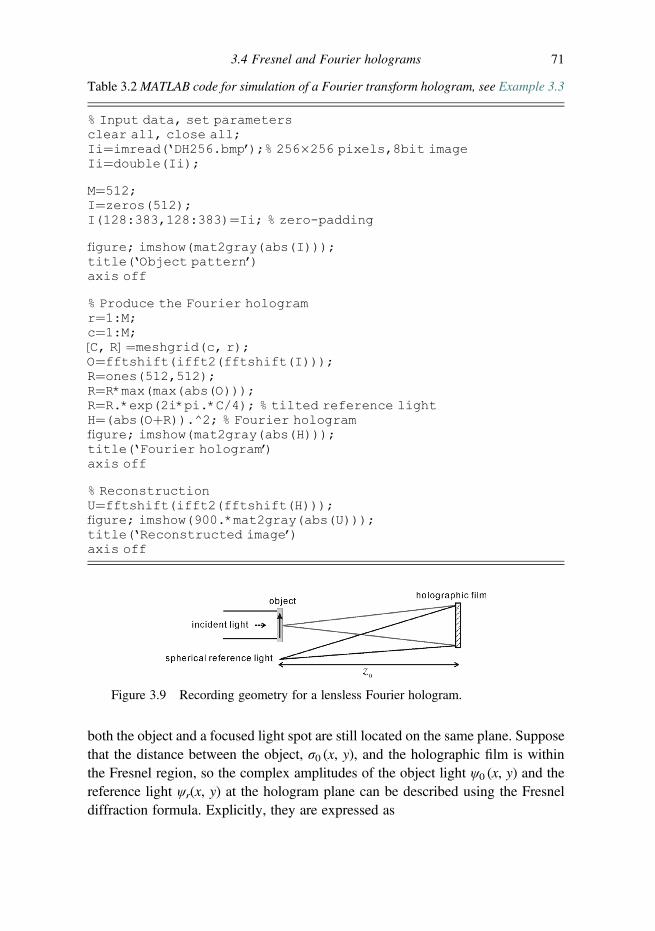
both the object and a focused light spot are still located on the same plane. Supposethat the distance between the object, σ0 (x, y), and the holographic film is withinthe Fresnel region, so the complex amplitudes of the object light ψ0 (x, y) and thereference light ψr(x, y) at the hologram plane can be described using the Fresneldiffraction formula. Explicitly, they are expressed as

Table 3.2MATLAB code for simulation of a Fourier transform hologram, see Example 3.3

% Input data, set parametersclear all, close all;Ii¼imread(‘DH256.bmp’);% 256�256 pixels,8bit imageIi¼double(Ii);

M¼512;I¼zeros(512);I(128:383,128:383)¼Ii; % zero-padding

figure; imshow(mat2gray(abs(I)));title(‘Object pattern’)axis off

% Produce the Fourier hologramr¼1:M;c¼1:M;[C, R]¼meshgrid(c, r);O¼fftshift(ifft2(fftshift(I)));R¼ones(512,512);R¼R*max(max(abs(O)));R¼R.*exp(2i*pi.*C/4); % tilted reference lightH¼(abs(OþR)).^2; % Fourier hologramfigure; imshow(mat2gray(abs(H)));title(‘Fourier hologram’)axis off

% ReconstructionU¼fftshift(ifft2(fftshift(H)));figure; imshow(900.*mat2gray(abs(U)));title(‘Reconstructed image’)axis off

Figure 3.9 Recording geometry for a lensless Fourier hologram.

3.4 Fresnel and Fourier holograms 71

ψ0 x, yð Þ ¼ exp−jk02z0

x2 þ y2 � �

� F σ0 x,yð Þexp −jk02z0

x2 þ y2 � ��

kx ¼ k0x

z0,

ky ¼ k0y

z0

ð3:14aÞ

ψrðx, yÞ ¼ exp−jk02z0

ðx2 þ y2Þ" #

� F

�δðx−x0,yÞexp −jk0

2z0ðx2 þ y2Þ

" #�kx ¼ k0x

z0,

ky ¼ k0y

z0

¼ exp

�−jk02z0

ðx−x0Þ2 þ y2h i�

, ð3:14bÞ

where z0 is the distance between the object and the hologram. Note that theproportional constants in ψ0 and ψr have been dropped for simplicity. The recordedhologram becomes

t x, yð Þ ¼ jψ0 x,yð Þ þ ψr x,yð Þj2:

Our concern is the cross terms upon holographic recording, which are

ψ0ðx, yÞψ�r ðx, yÞ þ ψ�

0ðx, yÞψrðx, yÞ ¼ exp−jk0x0x

z0þ jk0x20

2z0

!

� F

�σ0ðx,yÞexp −jk0

2z0ðx2 þ y2Þ

" #�kx¼

k0x

z0, ky ¼ k0y

z0

þexpjk0x0x

z0−jk0x202z0

!

�F

�σ0ðx,yÞexp −jk0

2z0ðx2 þ y2Þ

" #�kx¼

k0x

z0, ky ¼ k0y

z0

�:

ð3:15Þ

We can now use the setup shown in Fig. 3.7(b) to reconstruct the lensless Fourierhologram. Ignoring the zeroth-order light, the optical field at the back focal planeof the lens is


F fψ0ðx,yÞψ�r ðx,yÞ þ ψ�

0ðx,yÞψrðx,yÞgkx¼

k0x

f,ky ¼ k0y

f

/ σ0 −z0fxþ x0, −

z0fy

!

�exp

(−jk02z0

ðz0fx−x0Þ2 þ ðz0

fyÞ2

" #)þ σ�0

z0fxþ x0,

z0fy

!

�exp

(jk02z0

ðz0fxþ x0Þ2 þ ðz0

fyÞ2

" #), ð3:16Þ

where we have neglected any constant factors. Again, we obtain an invertedimage at x ¼ fx0 / z0, y ¼ 0, and a conjugate image at x ¼ −fx0 / z0, y ¼ 0.Note that there is an additional quadratic phase among the reconstructedimages. So the reconstruction method only applies to the display of intensityimages.

3.5 Rainbow hologram

The rainbow hologram, invented by Benton [7], is one of the easiest techniquesto produce a monochromatic reconstructed image using white light reconstruc-tion. The recording of the rainbow hologram contains two steps. First we recorda conventional off-axis hologram with a reference light at angle θ with respect tothe z-axis, as shown in Fig. 3.10(a). In the second step, we use reconstructionlight at angle −θ to illuminate the first hologram, producing a real image of theobject on axis [see Problem 3.2]. Such reconstruction light is called a conjugatebeam. However, the real image is reconstructed using a very small aperture ofthe hologram as a narrow horizontal slit is placed next to the hologram. Withthis aperture-reduced real image, we record another hologram as shown inFig. 3.10(b). The resulting hologram is the desired rainbow hologram. In thereconstruction process, we use a white conjugate reference beam to illuminatethe rainbow hologram, i.e., being conjugate to the reference light used to recordthe second hologram. The slit together with the real image of the object isreconstructed. In other words, all the diffracted light converges to the location ofthe slit, forming a bright slit image. Because of the inherent chromatic aberrationof the hologram, the slit images for different colors are separated vertically.If the observer’s eyes locate the slit image, a bright, monochromatic recon-structed image can be seen. The color of the image changes gradually from redto blue as the eyes move vertically. Because the two-step recording processis complicated, a one-step recording technique for the rainbow hologram has

3.5 Rainbow hologram 73

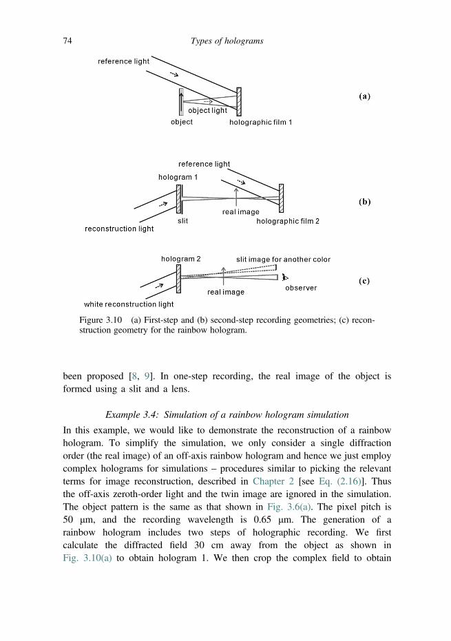
been proposed [8, 9]. In one-step recording, the real image of the object isformed using a slit and a lens.

Example 3.4: Simulation of a rainbow hologram simulation

In this example, we would like to demonstrate the reconstruction of a rainbowhologram. To simplify the simulation, we only consider a single diffractionorder (the real image) of an off-axis rainbow hologram and hence we just employcomplex holograms for simulations – procedures similar to picking the relevantterms for image reconstruction, described in Chapter 2 [see Eq. (2.16)]. Thusthe off-axis zeroth-order light and the twin image are ignored in the simulation.The object pattern is the same as that shown in Fig. 3.6(a). The pixel pitch is50 μm, and the recording wavelength is 0.65 μm. The generation of arainbow hologram includes two steps of holographic recording. We firstcalculate the diffracted field 30 cm away from the object as shown inFig. 3.10(a) to obtain hologram 1. We then crop the complex field to obtain

Figure 3.10 (a) First-step and (b) second-step recording geometries; (c) recon-struction geometry for the rainbow hologram.


a slit-aperture hologram, which is illuminated by a conjugate beam to give thefield propagated at a distance of 60 cm to obtain hologram 2 [see Fig. 3.10(b)].Finally, we reconstruct hologram 2 by a conjugate beam by allowing the propa-gation of 30 cm to get the real image “DH” in Fig. 3.10(c) and then another30 cm to reach the observer’s pupil. In the reconstruction, we use three differentcolors of light, R (λ ¼ 650 nm), G (λ ¼ 550 nm), and B (λ ¼ 450 nm), toilluminate the hologram [Fig. 11(a–c)]. The slit images of the three colors in theobserver plane are separated. Hence if the eye level of the observer moves upor down vertically, he or she will see the reconstructed image with a differentcolor. This is also why the technique is called “rainbow holography.” Thus onlylight with a single wavelength or with a narrow bandwidth of the reconstructedlight can pass through the small pupil of the observer. Indeed Fig. 3.11(d)shows the reconstructed image of a single wavelength. Because of the maskeffect of the slit, the resolution of the reconstructed image is worse than thatof the conventional holographic image. This is a shortcoming of rainbow holog-raphy [10, 11]. The MATLAB code of the example is listed in Table 3.3 as areference.

Figure 3.11 Reconstruction of the rainbow hologram. (a)–(c) The slitimages for B (λ ¼ 450 nm), G (λ ¼ 550 nm), and R (λ ¼ 650 nm) colorsat the observer’s plane, respectively. The arrows indicate the altitude ofthe observer’s eyes. (d) The reconstructed image at the object plane for the Rcolor.

3.5 Rainbow hologram 75

Table 3.3 MATLAB code for simulation of a rainbow hologram, see Example 3.4

% Input data, set parametersclear all, close all;Ii¼imread(‘DH256.bmp’);% 256�256 pixels 8bit imageIi¼double(Ii);PH¼rand([256,256]);Ii¼Ii.*exp(2i*pi*PH); % random phase on the object pattern

% 1. Forward propagation to hologram 1M¼256;z¼30; %(cm, distance between object and observer)w¼6500*10^-8; %(cm, wavelength)delta¼0.005; %(cm, pixel pitch 50um)r¼1:M;c¼1:M;[C, R]¼meshgrid(c, r);p¼exp(-2i*pi*z.*((1/w)^2-(1/M/delta)^2.*(C-M/2-1).^2-. . .(1/M/delta)^2.*(R-M/2-1).^2).^0.5);

A0¼fftshift(ifft2(fftshift(Ii)));Az¼A0.*p;E¼fftshift(fft2(fftshift(Az)));ES¼zeros(512);ES(246:265,128:383)¼E(118:137,:); % A slit aperture

% 2.Forward propagation to hologram 2M¼512;r¼1:M;c¼1:M;[C, R]¼meshgrid(c, r);A1¼fftshift(ifft2(fftshift(conj(ES))));z¼60; % distance between hologram 1 and hologram 2p¼exp(-2i*pi*z.*((1/w)^2-(1/M/delta)^2.*(C-M/2-1).^2-. . .(1/M/delta)^2.*(R-M/2-1).^2).^0.5);

Az1¼A1.*p;H¼fftshift(fft2(fftshift(Az1)));% object light at the hologram plane

% 3.Reconstruction (650nm)H2¼zeros(1024);H2(256:767,256:767)¼conj(H);M¼1024;r¼1:M;c¼1:M;[C, R]¼meshgrid(c, r);z¼30;p¼exp(-2i*pi*z.*((1/w)^2-(1/M/delta)^2.*(C-M/2-1).^2-. . .(1/M/delta)^2.*(R-M/2-1).^2).^0.5);

A2¼fftshift(ifft2(fftshift(H2)));Az2¼A2.*p;R650¼fftshift(fft2(fftshift(Az2)));R650¼(abs(R650)).^2;R650¼R650/max(max(R650));R650¼R650(384:639,384:639);figure; imshow(R650);

Table 3.3 (cont.)

title(‘Reconstructed image(650nm)’)axis off

Az2¼Az2.*p; % at observer planeS650¼fftshift(fft2(fftshift(Az2)));S650¼(abs(S650)).^2;S650¼S650/max(max(S650));S650¼S650(384:639,384:639);

% Reconstruction (550nm)w2¼5500*10^-8;H3¼H2.*exp(2i*pi*sind(0.4)*(w-w2)/w/w2.*R*delta);p¼exp(-2i*pi*z.*((1/w2)^2-(1/M/delta)^2.*(C-M/2-1).^2-. . .

(1/M/delta)^2.*(R-M/2-1).^2).^0.5);Az3¼fftshift(ifft2(fftshift(H3))).*p;R550¼fftshift(fft2(fftshift(Az3)));R550¼(abs(R550)).^2;R550¼R550/max(max(R550));R550¼R550(384:639,384:639);figure; imshow(R550);title(‘Reconstructed image (550nm)’)

Az3¼Az3.*p;S550¼fftshift(fft2(fftshift(Az3)));S550¼(abs(S550)).^2;S550¼S550/max(max(S550));S550¼S550(384:639,384:639);

% Reconstruction (450nm)w3¼4500*10^-8;H4¼H2.*exp(2i*pi*sind(0.4)*(w-w3)/w/w3.*R*delta);p¼exp(-2i*pi*z.*((1/w3)^2-(1/M/delta)^2.*(C-M/2-1).^2-. . .

(1/M/delta)^2.*(R-M/2-1).^2).^0.5);Az4¼fftshift(ifft2(fftshift(H4))).*p;R450¼fftshift(fft2(fftshift(Az4)));R450¼(abs(R450)).^2;R450¼R450/max(max(R450));R450¼R450(384:639,384:639);figure; imshow(R450);title(‘reconstructed image (450nm)’)

Az4¼Az4.*p;S450¼fftshift(fft2(fftshift(Az4)));S450¼(abs(S450)).^2;S450¼S450/max(max(S450));S450¼S450(384:639,384:639);

% color slit imageSLIT¼zeros(256,256,3);SLIT(:,:,1)¼S650;SLIT(:,:,2)¼S550;SLIT(:,:,3)¼S450;SLIT¼uint8(SLIT.*500);figure; image(SLIT)title(‘Slit images’)axis offaxis equal

Problems

3.1 When the off-axis hologram is reconstructed with a light beam by the originalreferencewave [see Fig. 3.3(b)], the virtual image appears on-axis in the positionof the original object and the real image is formed off-axis. Let us reconstructthe hologram with a light beam propagating at an angle −θ to the z-axis, i.e., weare using a conjugate beam to reconstruct the hologram. Show that the recon-structed real image is on-axis and the virtual image appears off-axis.

3.2 Verify that in lensless Fourier holography as discussed in Fig. 3.9, the recon-structed images are separated by 2fx0 / z0, where f is the focal length of the lensused for reconstruction, x0 is the separation distance between the sphericalreference light and the object. In other words, you need to verify Eq. (3.16).

3.3 Consider an off-axis hologram. We assume that the object is at the optical axisand is z0 behind the hologram. The offset angle of the plane wave referencelight is θ0, and the recording wavelength is λ0. If the reconstruction light is also aplane wave with an offset angle θ0 but with a wavelength of λr, show that thelocation of the reconstructed image is at (zr (λ0/λr) z0; xr z0tanθ0(1 − λ0/λr)).

3.4 Assume that the slit for generating a rainbow hologram is z0 from thehologram plane, and the offset angle of the plane wave reference light is θ0.The recording wavelength is λ0. With reference to Fig. 3.10(c), show that therelationship between the width of the slit, w, the diameter of the observer’spupil, d, and the bandwidth, Δλ, of the reconstructed image is given by Δλ λ0(w þ d)/z0tanθ0.

References

1. R. J. Collier, C. B. Burckhardt, and L. H. Lin, Optical Holography (Murray Hill, NJ,1983).

2. P. Hariharan, Optical Holography: Principles, Techniques, and Applications(Cambridge University Press, Cambridge, 1996).

3. P. Hariharan, Basics of Holography (Cambridge University Press, Cambridge, 2002).4. S. A. Benton, and V. M. B. Jr., Holographic Imaging (Wiley, Hoboken, NJ, 2008).5. D. Garbor, A new microscopic principle, Nature 161, 777–778 (1948).6. E. N. Leith, and J. Upatnieks, Reconstructed wavefronts and communication theory,

Journal of the Optical Society of America 52, 1123–1130 (1962).7. S. A. Benton, Hologram reconstructions with extended incoherent sources, Journal of

the Optical Society of America 59, 1545–1546 (1969).8. H. Chen, and F. T. S. Yu, One-step rainbow hologram, Optics Letters 2, 85–87 (1978).9. H. Chen, A. Tai, and F. T. S. Yu, Generation of color images with one-step rainbow

holograms, Applied Optics 17, 1490–1491 (1978).10. J. C. Wyant, Image blur for rainbow holograms, Optics Letters 1, 130–132 (1977).11. E. N. Leith, and H. Chen, Deep-image rainbow holograms, Optics Letters 2, 82–84

(1978).


4

Conventional digital holography

In Chapter 3 we introduced the fundamental theory of optical holographyand reviewed several conventional holographic recording schemes. In digitalholography, the recording schemes are the same, but the recording material isreplaced by an electronic device, such as a charge-coupled device (CCD). Opticalinterference fringes acquired by the CCD are digitized into a two-dimensionaldigital signal and then processed using digital image processing to reconstructthe hologram. Figure 4.1(a) shows a typical case of digital holography and inthis chapter we concentrate on this case. However, we may also come across othersituations in digital holography. Complete numerical simulations of hologramconstruction and reconstruction can be performed purely by digital methods, asshown in Fig. 4.1(b).

We can also produce a digital hologram without any optical interference(i.e., a computer-generated hologram, see Chapter 7 for details). The hologram canthen be sent to a display device for optical reconstruction, as shown in Fig. 4.1(c).In each of these situations, we need to simulate interference between the object andthe hologram in the front end, and then simulate diffraction between the hologramand the diffraction plane or the observation plane in the back end of the overallprocess. Because creating the digital signal and digital calculations of diffractionare the core of digital holography, in this chapter we will first introduce the conceptof discrete signals and their corresponding calculations for readers who are notfamiliar with digital signals and systems. Then we will discuss the propertiesand limitations of the recording device, i.e., a CCD. Finally, we will develop thediscrete version of diffraction formulas and discuss any related problems.

4.1 Sampled signal and discrete Fourier transform

Details of digital signals and systems are beyond the scope of the book, so wewill only discuss the most important properties that will be involved in digital

79

holography. In the following discussion we treat only the one-dimensional case forsimplicity without any loss of generality.

Assuming f (x) is a continuous analog signal along the x-axis, we can producea discrete signal corresponding to f (x) by sampling it with a fixed separation, Δx,

f n½ � ¼ f nΔxð Þ ¼XN−1k¼0

f kΔxð Þ • δð½n−k� • ΔxÞ, ð4:1Þ

Figure 4.1 Three forms of digital holography.

80 Conventional digital holography

where n is an integer between 0 and (N − 1), and δ(n) is the unit impulse sequence,which is the counterpart of the delta function when dealing with discrete signals.The mathematical definition of δ([n − k]Δx) is

δ ½n−k�Δxð Þ ¼ 1 n ¼ k0 n 6¼ k:

�ð4:2Þ

In Eq. (4.1) we have also assumed that f (x) is zero outside the range 0 � x < NΔx

so that we can use a finite number of samplings, say N, to represent the originalanalog signal. Because the original signal is sampled with sampling period Δx,the sampling frequency is fs¼ 1/Δx. In the following discussion we assume thatN is even for the sake of simplicity, although it is not limited to being even. Also tosimplify the discussion, we ignore the problem of finding the spectrum of a discretesignal. We must, however, know two important properties. First, the spectrumof the sampled signal f [n] is periodic in the spectrum domain. This concept canbe easily grasped in the analog version. By applying the Fourier transform to acontinuous-defined sampled function, we get

F f ðxÞ�X∞n¼−∞

δðx−nΔxÞ( )

¼ 2πfsX∞n¼−∞

Fðkx−2πfsnÞ, ð4:3Þ

where F kxð Þ ¼ F f ðxÞf g. Thus the spectrum of the sampled function consists ofthe spectrum of the unsampled function which is replicated every 2πfs radian/second. Assuming that the duplicates do not overlap with each other, the spec-trum of the sampled function is periodic with period 2πfs, as shown in Fig. 4.2. Sowe can select any region of the spectrum with length 2πfs to represent thecomplete spectrum information.

The interval over which the analog signal is sampled is referred to as the recordlength, Lx. With the number of samples N, the following relationships hold:

Lx ¼ NΔx ¼ N=fs and Δf ¼ 1=Lx ¼ fs=N, ð4:4Þwhere Δf is the frequency resolution. In other words, for a given number ofsample points, N, and sampling period, Δx, the sampling resolution in thefrequency domain, Δf, is fixed. The resulting extent in the frequency domain isLf¼ 1/Δx.

To understand the above relationships, let us assume that the continuous signalf (x) is sampled over the length Lx¼NΔx. Hence the spectrum of the continuoussignal can be expressed as

F f ðxÞ�rectx

Lx

� �� ¼ F kxð Þ � Lx sinc kxLx

2π

� �: ð4:5Þ

4.1 Sampled signal and discrete Fourier transform 81

Since the resulting spectrum is the convolution of the original spectrum F(kx) andthe sinc function, the sinc function can be regarded as an impulse response ofa system with the original spectrum F(kx) treated as an input. Therefore the widthof the impulse response defines the “frequency” resolution of the system.The “width,” Δk, of sinc(kxLx/2π) can be defined by setting the argument ofthe sinc function to 1, i.e., the first zero of the sinc function, giving the widthΔk¼ 2π/Lx¼ 2π/NΔx or Δf¼ 1/NΔx¼ 1/Lx. So when the samples are Δf apart inthe spectral domain, the value of Δf gives the frequency resolution of theresulting Fourier transform.

Now, for convenience, the frequency range of the spectrum is usuallyselected to be [0, fs) (this expression means 0 is included but fs is not included)in the unit of cycle/length, or [0, 2πfs) in the unit of radian/length. Accordingly,the discrete spectrum F[m] can be found from f[n] by the discrete Fouriertransform (DFT),

F m½ � ¼XN−1n¼0

f n½ �•exp −j2πnmN

� �, ð4:6aÞ

where m is an integer, being also between 0 and (N − 1). Note that F[m] is theN-point DFT of f [n] and is itself a periodic sequence with period equal to N.Similar to the Fourier transform of a continuous signal, we can retrieve f [n] fromF[m] by the inverse discrete Fourier transform (IDFT),

f n½ � ¼ 1N •

XN−1m¼0

F m½ �•exp j2πnmN

� �: ð4:6bÞ

Figure 4.2 Spectrum of (a) the original continuous function, f (x), and (b) thesampled function.


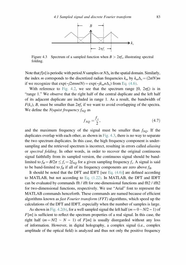
Note that f[n] is periodicwith periodN samples orNΔx in the spatial domain. Similarly,the index m corresponds to the discretized radian frequencies km by kmΔx¼ (2π/N)mif we recognize that exp(−j2πnm/N)¼ exp(−jkmnΔx) from Eq. (4.6).

With reference to Fig. 4.2, we see that the spectrum range [0, 2πfs) is in“range 1.” We observe that the right half of the central duplicate and the left halfof its adjacent duplicate are included in range 1. As a result, the bandwidth ofF(kx), B, must be smaller than 2πfs if we want to avoid overlapping of the spectra.We define the Nyquist frequency fNQ as

f NQ ¼ f s2, ð4:7Þ

and the maximum frequency of the signal must be smaller than fNQ. If theduplicates overlap with each other, as shown in Fig. 4.3, there is no way to separatethe two spectrum duplicates. In this case, the high frequency component is under-sampling and the retrieved spectrum is incorrect, resulting in errors called aliasingor spectral folding. In other words, in order to recover the original continuoussignal faithfully from its sampled version, the continuous signal should be band-limited to fB¼B/2π � fs¼ 2fNQ for a given sampling frequency fs. A signal is saidto be band-limited to fB if all of its frequency components are zero above fB.

It should be noted that the DFT and IDFT [see Eq. (4.6)] are defined accordingto MATLAB, but not according to Eq. (1.22). In MATLAB, the DFT and IDFTcan be evaluated by commands fft / ifft for one-dimensional functions and fft2 / ifft2for two-dimensional functions, respectively. We use “Arial” font to represent theMATLAB commands henceforth. These commands are named because of efficientalgorithms known as fast Fourier transform (FFT) algorithms, which speed up thecalculations of the DFT and IDFT, especially when the number of samples is large.

As shown in Fig. 4.2(b), for a well sampled signal the left half (m¼ 0 ~ N/2 − 1) ofF[m] is sufficient to reflect the spectrum properties of a real signal. In this case, theright half (m¼N/2 ~ N − 1) of F[m] is usually disregarded without any lossof information. However, in digital holography, a complex signal (i.e., complexamplitude of the optical field) is analyzed and thus not only the positive frequency

Figure 4.3 Spectrum of a sampled function when B > 2πfs, illustrating spectralfolding.


spectrum but also the negative frequency spectrum of F(kx) is necessary. In otherwords, we prefer to obtain the spectrum in range 2 rather than in range 1 in Fig. 4.2(b).Because the sampling period of f [n] is 1/Δx and the command fft generates thespectrum of the signal in the range given by [0, 2πfs), we have the distribution ofthe spectrum in the range kx¼ 2π(N/2 − 1)/NΔx ~ 2π(N − 1)/NΔx, which is the same asthat in the range kx¼ 2π(−N/2 − 1)/NΔx ~ 2π(−1)/NΔx. As a result, the full frequencyspectrum between�πfs can be obtained directly by swapping the right and left halvesof F[m]. After the swap, the spectrum is represented in�πfs, or (m¼−N/2 ~ N/2 − 1),and the zero frequency (m¼ 0) locates at the (N/2 þ 1) point of the swappedspectrum. In MATLAB, we can use the command fftshift to swap the data. Readersmay also apply the command ifftshift, which is useful if the data number is odd.

Example 4.1: Under-sampling and aliasing

In this example we will see the effect of aliasing. We sample a sine function sin(2πx/5), where x is in millimeters. The period of the function is 5 mm. Accordingto the sampling theorem, the sampling period must be smaller than 2.5 mm in orderto avoid aliasing. We use 0.1 mm, 0.2 mm, 0.4 mm, and 3 mm as the differentsampling periods. The sampled data are then transformed to the spectral domain sothat we can measure the frequency of the signal directly. In the continuous spatialdomain, using a one-dimensional version of the two-dimensional Fourier transform[see Eq. 1.22)], we can find that

F sinð2πx=5Þf g ¼ j½πδ kx þ 2π=5ð Þ−πδ kx−2π=5ð Þ�:Therefore, we expect to have two “peaks” at kx¼�2π/5 rad/mm or at 1/5¼ 0.2 mm−1

in the magnitude spectrum, i.e., jF sinð2πx=5Þf gj, of the signal. The magnitudespectra are plotted in Fig. 4.4 (a) to (c) for the sampling periods of 0.1 mm, 0.2 mm,and 0.4 mm, respectively, and we observe that the two peaks in the spectrum arealways at 0.2mm−1, which corresponds to the correct signal of period 5mm.When thesampling period is 3 mm, the peaks of the spectrum are at�0.133 mm−1 [Fig. 4.4(d)],which is incorrect due to aliasing. The MATLAB code is listed in Table 4.1.

Example 4.2: Sampling

We have an analog signal f (x) that is bandlimited to 100 cycle/mm. The signal isto be sampled at the Nyquist frequency. The frequency resolution required is tobe at 0.1 cycle/mm. Find the record length and the number of samples.

The Nyquist frequency is fNQ¼ 2�100 cycle/mm¼ 200 cycle/mm.To achieve a frequency resolution of 0.5 cycle/mm, the total record length isLx¼ 1/Δf¼ 1/0.1¼ 10mm. The resulting number of samples is thenN¼ Lx fNQ¼ 10�200¼ 2000 samples.


Example 4.3: Fourier transform of a rectangular function

We use a rectangular function and its Fourier transform as an example to show theimplementation of the DFT using MATLAB. Table 4.2 is the MATLAB code andFig. 4.5 shows the simulation results. At the first step, we center the aperture to theorigin of the axis, which is at the (N/2þ1) point of f [n]. Then we apply commandfftshift to f [n] so that the origin of the axis is re-located to the first point, which isthe requirement of the DFT (or IDFT) using MATLAB. Meanwhile, the –x portionof the rectangular function is moved to þx. This can be done because the periodof the phase in Eq. (4.6a) is N sampling points,

exp −j2πðnþ NÞm

N

� �¼ exp −

j2πnmN

� �•exp −

j2πNmN

� �¼ exp −

j2πnmN

� �: ð4:8Þ

Therefore in the DFT the phase contribution of the point at –x is identical to that ofthe point at (–xþNΔx), which is what we do using fftshift. After the spectrum hasbeen calculated using command fft, we perform fftshift again to re-locate the originof the spectrum domain at the center of the axis, i.e., the (N/2þ1) point.

Figure 4.4 Magnitude spectra of a sine function sampled with periods at(a) 0.1 mm, (b) 0.2 mm, (c) 0.4 mm, and (d) 3 mm. The measured spatialfrequencies are 0.2 mm−1 (a–c) and 0.133 mm−1 (d).


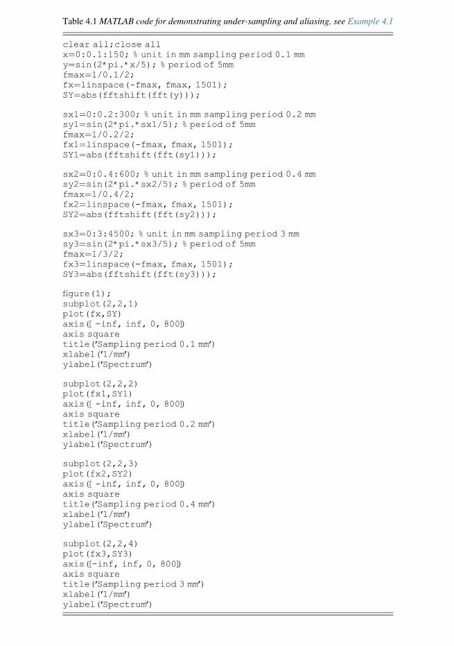
Table 4.1 MATLAB code for demonstrating under-sampling and aliasing, see Example 4.1

clear all;close allx¼0:0.1:150; % unit in mm sampling period 0.1 mmy¼sin(2*pi.*x/5); % period of 5mmfmax¼1/0.1/2;fx¼linspace(-fmax, fmax, 1501);SY¼abs(fftshift(fft(y)));

sx1¼0:0.2:300; % unit in mm sampling period 0.2 mmsy1¼sin(2*pi.*sx1/5); % period of 5mmfmax¼1/0.2/2;fx1¼linspace(-fmax, fmax, 1501);SY1¼abs(fftshift(fft(sy1)));

sx2¼0:0.4:600; % unit in mm sampling period 0.4 mmsy2¼sin(2*pi.*sx2/5); % period of 5mmfmax¼1/0.4/2;fx2¼linspace(-fmax, fmax, 1501);SY2¼abs(fftshift(fft(sy2)));

sx3¼0:3:4500; % unit in mm sampling period 3 mmsy3¼sin(2*pi.*sx3/5); % period of 5mmfmax¼1/3/2;fx3¼linspace(-fmax, fmax, 1501);SY3¼abs(fftshift(fft(sy3)));

figure(1);subplot(2,2,1)plot(fx,SY)axis([-inf, inf, 0, 800])axis squaretitle(’Sampling period 0.1 mm’)xlabel(’1/mm’)ylabel(’Spectrum’)

subplot(2,2,2)plot(fx1,SY1)axis([-inf, inf, 0, 800])axis squaretitle(’Sampling period 0.2 mm’)xlabel(’1/mm’)ylabel(’Spectrum’)

subplot(2,2,3)plot(fx2,SY2)axis([-inf, inf, 0, 800])axis squaretitle(’Sampling period 0.4 mm’)xlabel(’1/mm’)ylabel(’Spectrum’)

subplot(2,2,4)plot(fx3,SY3)axis([-inf, inf, 0, 800])axis squaretitle(’Sampling period 3 mm’)xlabel(’1/mm’)ylabel(’Spectrum’)

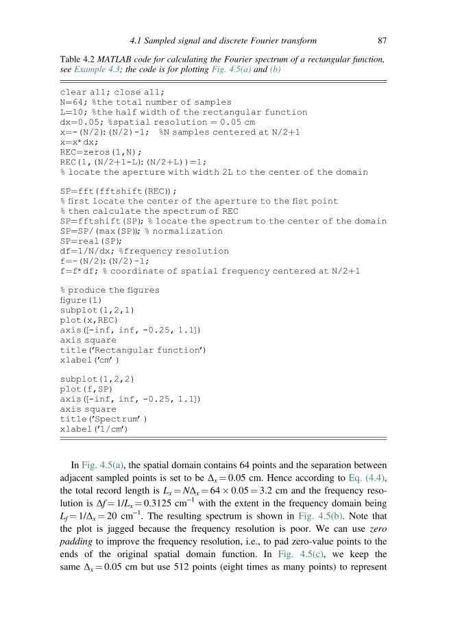
In Fig. 4.5(a), the spatial domain contains 64 points and the separation betweenadjacent sampled points is set to be Δx¼ 0.05 cm. Hence according to Eq. (4.4),the total record length is Lx¼NΔx¼ 64� 0.05¼ 3.2 cm and the frequency reso-lution is Δf¼ 1/Lx¼ 0.3125 cm−1 with the extent in the frequency domain beingLf¼ 1/Δx¼ 20 cm−1. The resulting spectrum is shown in Fig. 4.5(b). Note thatthe plot is jagged because the frequency resolution is poor. We can use zeropadding to improve the frequency resolution, i.e., to pad zero-value points to theends of the original spatial domain function. In Fig. 4.5(c), we keep thesame Δx¼ 0.05 cm but use 512 points (eight times as many points) to represent

Table 4.2 MATLAB code for calculating the Fourier spectrum of a rectangular function,see Example 4.3; the code is for plotting Fig. 4.5(a) and (b)

clear all; close all;N¼64; %the total number of samplesL¼10; %the half width of the rectangular functiondx¼0.05; %spatial resolution ¼ 0.05 cmx¼-(N/2):(N/2)-1; %N samples centered at N/2þ1x¼x*dx;REC¼zeros(1,N);REC(1,(N/2þ1-L):(N/2þL))¼1;% locate the aperture with width 2L to the center of the domain

SP¼fft(fftshift(REC));% first locate the center of the aperture to the fist point% then calculate the spectrum of RECSP¼fftshift(SP); % locate the spectrum to the center of the domainSP¼SP/(max(SP)); % normalizationSP¼real(SP);df¼1/N/dx; %frequency resolutionf¼-(N/2):(N/2)-1;f¼f*df; % coordinate of spatial frequency centered at N/2þ1

% produce the figuresfigure(1)subplot(1,2,1)plot(x,REC)axis([-inf, inf, -0.25, 1.1])axis squaretitle(’Rectangular function’)xlabel(’cm’)

subplot(1,2,2)plot(f,SP)axis([-inf, inf, -0.25, 1.1])axis squaretitle(’Spectrum’)xlabel(’1/cm’)


Figure 4.5 Rectangular function (left) and its Fourier spectrum (right). Thespatial resolution and sample numbers of (a), (c), (e) are (Δx, N) ¼ (0.05 cm,64), (0.05 cm, 512), and (0.00625 cm, 512), respectively.


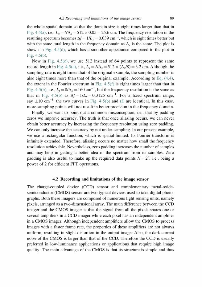
the whole spatial domain so that the domain size is eight times larger than that inFig. 4.5(a), i.e., Lx¼NΔx¼ 512� 0.05¼ 25.6 cm. The frequency resolution in theresulting spectrum becomes Δf¼ 1/Lx¼ 0.039 cm−1, which is eight times better butwith the same total length in the frequency domain as Δx is the same. The plot isshown in Fig. 4.5(d), which has a smoother appearance compared to the plot inFig. 4.5(b).

Now in Fig. 4.5(e), we use 512 instead of 64 points to represent the samerecord length in Fig. 4.5(a), i.e., Lx¼NΔx¼ 512� (Δx/8)¼ 3.2 cm. Although thesampling rate is eight times that of the original example, the sampling number isalso eight times more than that of the original example. According to Eq. (4.4),the extent in the Fourier spectrum in Fig. 4.5(f) is eight times larger than that inFig. 4.5(b), i.e., Lf¼ 8/Δx¼ 160 cm−1, but the frequency resolution is the same asthat in Fig. 4.5(b) as Δf¼ 1/Lx¼ 0.3125 cm−1. For a fixed spectrum range,say �10 cm−1, the two curves in Fig. 4.5(b) and (f) are identical. In this case,more sampling points will not result in better precision in the frequency domain.

Finally, we want to point out a common misconception, i.e., that by paddingzeros we improve accuracy. The truth is that once aliasing occurs, we can neverobtain better accuracy by increasing the frequency resolution using zero padding.We can only increase the accuracy by not under-sampling. In our present example,we use a rectangular function, which is spatial-limited. Its Fourier transform isinfinitely extended. Therefore, aliasing occurs no matter how small the frequencyresolution achievable. Nevertheless, zero padding increases the number of samplesand may help in getting a better idea of the spectrum from its samples. Zeropadding is also useful to make up the required data points N¼ 2n, i.e., being apower of 2 for efficient FFT operations.

4.2 Recording and limitations of the image sensor

The charge-coupled device (CCD) sensor and complementary metal-oxide-semiconductor (CMOS) sensor are two typical devices used to take digital photo-graphs. Both these imagers are composed of numerous light sensing units, namelypixels, arranged as a two-dimensional array. The main difference between the CCDimager and the CMOS imager is that the signal from all the pixels shares one orseveral amplifiers in a CCD imager while each pixel has an independent amplifierin a CMOS imager. Although independent amplifiers allow the CMOS to processimages with a faster frame rate, the properties of these amplifiers are not alwaysuniform, resulting in slight distortion in the output image. Also, the dark currentnoise of the CMOS is larger than that of the CCD. Therefore the CCD is usuallypreferred in low-luminance applications or applications that require high imagequality. The main advantage of the CMOS is that its structure is simple and thus

4.2 Recording and limitations of the image sensor 89

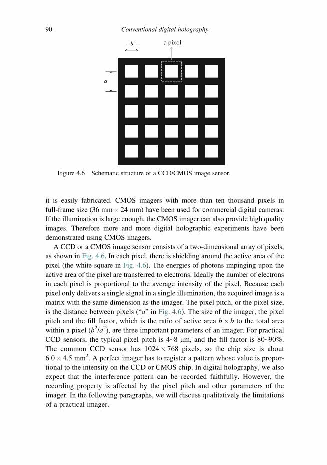
it is easily fabricated. CMOS imagers with more than ten thousand pixels infull-frame size (36 mm� 24 mm) have been used for commercial digital cameras.If the illumination is large enough, the CMOS imager can also provide high qualityimages. Therefore more and more digital holographic experiments have beendemonstrated using CMOS imagers.

A CCD or a CMOS image sensor consists of a two-dimensional array of pixels,as shown in Fig. 4.6. In each pixel, there is shielding around the active area of thepixel (the white square in Fig. 4.6). The energies of photons impinging upon theactive area of the pixel are transferred to electrons. Ideally the number of electronsin each pixel is proportional to the average intensity of the pixel. Because eachpixel only delivers a single signal in a single illumination, the acquired image is amatrix with the same dimension as the imager. The pixel pitch, or the pixel size,is the distance between pixels (“a” in Fig. 4.6). The size of the imager, the pixelpitch and the fill factor, which is the ratio of active area b� b to the total areawithin a pixel (b2/a2), are three important parameters of an imager. For practicalCCD sensors, the typical pixel pitch is 4~8 μm, and the fill factor is 80~90%.The common CCD sensor has 1024� 768 pixels, so the chip size is about6.0� 4.5 mm2. A perfect imager has to register a pattern whose value is propor-tional to the intensity on the CCD or CMOS chip. In digital holography, we alsoexpect that the interference pattern can be recorded faithfully. However, therecording property is affected by the pixel pitch and other parameters of theimager. In the following paragraphs, we will discuss qualitatively the limitationsof a practical imager.

Figure 4.6 Schematic structure of a CCD/CMOS image sensor.


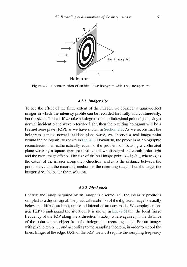
4.2.1 Imager size

To see the effect of the finite extent of the imager, we consider a quasi-perfectimager in which the intensity profile can be recorded faithfully and continuously,but the size is limited. If we take a hologram of an infinitesimal point object using anormal incident plane wave reference light, then the resulting hologram will be aFresnel zone plate (FZP), as we have shown in Section 2.2. As we reconstruct thehologram using a normal incident plane wave, we observe a real image pointbehind the hologram, as shown in Fig. 4.7. Obviously, the problem of holographicreconstruction is mathematically equal to the problem of focusing a collimatedplane wave by a square-aperture ideal lens if we disregard the zeroth-order lightand the twin image effects. The size of the real image point is ~λz0/Dx, where Dx isthe extent of the imager along the x-direction, and z0 is the distance between thepoint source and the recording medium in the recording stage. Thus the larger theimager size, the better the resolution.

4.2.2 Pixel pitch

Because the image acquired by an imager is discrete, i.e., the intensity profile issampled as a digital signal, the practical resolution of the digitized image is usuallybelow the diffraction limit, unless additional efforts are made. We employ an on-axis FZP to understand the situation. It is shown in Eq. (2.5) that the local fringefrequency of the FZP along the x-direction is x/λz0, where again z0 is the distanceof the point source object from the holographic recording plane. For an imagerwith pixel pitch ΔxCCD and according to the sampling theorem, in order to record thefinest fringes at the edge, Dx/2, of the FZP, we must require the sampling frequency

Figure 4.7 Reconstruction of an ideal FZP hologram with a square aperture.


fs ¼ 1=ΔxCCD � 2�ðDx=2Þ=λz0 ð4:9Þor

z0 � ΔxCCDDx

λ0: ð4:10Þ

Consequently, the reconstructed size of the real image point when the hologram issampled by the imager is the same as that in the analog case, i.e., λz0/Dx. Therefore,in digital holography the pixel size is also the minimum achievable resolved sizeof the reconstructed image, provided that the normal-incident plane wave is usedas the reference light. The result in Eq. (4.10) shows that if the object distance, z0,is smaller than ΔxCCDDx=λ0, the finer structures of the FZP cannot be resolved andaliasing occurs.

4.2.3 Modulation transfer function

We have just discussed the resolution limit due to the imager size and the samplingperiod. However, the image fidelity cannot be evaluated directly in the aboveanalysis. Similar to a lens, the quality of an imager can be evaluated in terms of themodulation transfer function (MTF), which describes the relative frequencyresponse of the output image of a system. The MTF of an imager mostly dependson the structure of the imager [1–4]. First, the periodic shielding structure (Fig. 4.6)can be regarded as a mask. Thus, presented in a one-dimensional case for simpli-city, the effective illumination on the imager can be written as

I0xð Þ ¼ I xð Þ�m xð Þ, ð4:11Þ

where I(x) is the illumination pattern on the imager and m(x) is the intensitytransmittance of the mask. Upon illumination of the active layer of the imager,photons are absorbed and electrons are excited simultaneously. Depending onthe material used, the thickness of the active layer, and the wavelength of theillumination, excited electrons will laterally diffuse, resulting in an electron densityD(x) given by

D xð Þ ¼ βI0 ðxÞ � GðxÞ, ð4:12Þ

where G(x) represents a Gaussian point spread function due to lateral diffusion,and β is a coupling constant, denoting the efficiency of the conversion of theelectrons released by the light illumination. Finally, the signal from a single pixelof an imager is proportional to the integration of the illumination pattern on thepixel, which can be expressed as


ðx0þ γΔxCCD

2

x0−γΔxCCD

2

D xð Þdx, ð4:13Þ

where γ is a linear fill factor, which is defined by b/a, and the ratio is illustrated inFig. 4.6; x0 is the location of the considered pixel. Equation (4.13) can be re-writtenusing the convolution operation as

ð∞−∞

D xð Þ•rect x−x0

γΔxCCD

� �dx ¼ D x

0�

� rect x0

γΔxCCD

� �¼ S x

0�

: ð4:14Þ

Thus for a one-dimensional image sensor containing N pixels, the nth pixel’soutput signal (n¼1~N) can be expressed as

S n½ � ¼ SðnΔxCCDÞ ¼ D nΔxCCDð Þ � rect nΔxCCD

γΔxCCD

!" #

¼ β

�IðnΔxCCDÞ�mðnΔxCCDÞ

� �� GðnΔxCCDÞ � rect

nΔxCCD

γΔxCCD

!�,

or in analog form as

SðxÞ ¼ β IðxÞ�mðxÞ½ � � GðxÞ � rect x

γΔxCCD

� �� : ð4:15Þ

For simplicity, we neglect the mask effect, i.e., letting m(x)¼ 1, so that we candefine the modulation transfer function (MTF) as

MTF ¼ jF SðxÞf g=F βIðxÞf gj ¼ F GðxÞ � rect x

γΔxCCD

� �� ,

or

MTF ¼ jF GðxÞf g�sinc γΔxCCDkx=2πð Þj, ð4:16Þwhich shows that the rectangular function and G(x) always act as lowpass filtersfor the illuminating pattern. For Si-based CCD imagers under short-wavelengthillumination (λ < 0.8 μm), the diffusion effect is minor [G(x) � δ(x)] andthe integrating effect of the pixel [Eq. (4.13)] dominates. A simulated MTFbased on Eq. (4.16) (ΔxCCD ¼ 5 μm; γ ¼ 0:9; λ ¼ 0:63 μm) is plotted in Fig. 4.8.It shows that the MTF is not zero when the frequency is larger than the Nyquistfrequency fNQ, where fNQ has been calculated according to Eq. (4.7) and is


labeled in the figure. Aliasing will occur if the illumination pattern containsspatial frequencies beyond fNQ.

It is difficult to apply the advanced model, that is Eq. (4.15), to determinequantitatively the MTF of a specific CCD imager because we do not usually haveenough information on m(x) and G(x). However, the MTF of a CCD imager can bemeasured by several experimental methods, which have been discussed in Refs.[5–7]. For general-purpose CCD imagers, high spatial frequency components areattenuated because of the roll-off of the MTF. Moreover, the response for frequen-cies larger than fNQ is not zero, causing aliasing errors. Figure 4.9 shows aphotograph of a FZP taken by a CCD imager (Kodak KAI-2020M). The centralcircular patterns are the true FZP structures while the darker circular patterns on thefour sides are the false (aliasing) structures due to undersampling of fine fringes.

Figure 4.9 Photograph of a FZP taken by a CCD imager. Aliasing is clearlyshown with the four faded circular patterns around the FZP.

Figure 4.8 Simulated MTF curve for a CCD imager.


4.3 Digital calculations of scalar diffraction

4.3.1 Angular spectrum method (ASM)

In scalar diffraction theory [see Section 1.3], the diffracted field ψp(x, y;z) can beobtained from the incident field, ψp0(x, y), according to Eq. (1.27),

ψpðx, y; zÞ ¼ F −1 F ψp0 x, yð Þn o

�H ðkx, ky; zÞn o

, ð4:17Þ

where H ðkx, ky; zÞ is the spatial frequency transfer function (SFTF) [see Eq. (1.26)].Equation (4.17) is the basic formula of the angular spectrummethod (ASM), which isalso called the convolution method or the double Fourier transform method.

Suppose that the sampling period along the x-axis is Δx with total M samples,and that the sampling period along the y-axis is Δy with total N samples, then thediscrete version of Eq. (4.17) is expressed as

ψp m, n½ � ¼ DFT2D IDFT2D ψp0 m, n½ �n o

�H p, q½ �n o

, ð4:18Þ

where

H p, q½ � ¼ exp −jk0z

ffiffiffiffiffiffiffiffiffiffiffiffiffiffiffiffiffiffiffiffiffiffiffiffiffiffiffiffiffiffiffiffiffiffiffiffiffiffiffi1−

ðpΔkxÞ2k20

−ðqΔkyÞ2

k20

s" #ð4:19Þ

and, according to Eq. (4.4), Δkx and Δky are the frequency resolution (radian/unit oflength) corresponding to sampling periods Δx and Δy along the x- and y-directions,respectively. Hence Δkx¼ 2π/MΔx and Δky¼ 2π/NΔy. In Eq. (4.18), (m, n) and(p, q) are the indices of the samples at the spatial domain and the Fourierdomain, respectively. Thus their ranges are: −M/2 � m � M/2 − 1, −N/2 � n �N/2 − 1, −M/2� p�M/2 − 1, and −N/2� q� N/2 − 1. DFT2D{•} and IDFT2D{•}denote the two-dimensional discrete Fourier transform and the two-dimensionalinverse discrete Fourier transform, respectively, and they are defined as

DFT2D f m, n½ �f g ¼ F p, q½ � ¼XM2−1m¼−M2

XN2−1n¼−N2

f m, n½ �•exp −j2πpm

Mþ qn

N

� h i, ð4:20aÞ

IDFT2D F½p, q�f g ¼ f m, n½ � ¼XM2−1p¼−M2

XN2−1q¼−N2

F½ p, q�•exp j2πpm

Mþ qn

N

� h i: ð4:20bÞ

Example 4.4: Diffraction of a rectangular aperture

In this example we simulate the diffraction of a rectangular aperture using theASM. Table 4.3 gives the corresponding MATLAB code. In MATLAB, the

4.3 Digital calculations of scalar diffraction 95

command fftshift(fft2(fftshift(.))) performs DFT2D{•}, and fftshift(ifft2(fftshift(.)))calculates IDFT2D{•}. We perform fftshift before and after calculating fft2 (ifft2)in MATLAB because the origins in Eqs. (4.18), (4.19), and (4.20) are at the centerof the coordinates. Also, the output from fft2 (ifft2) always gives the first point atthe origin of the coordinates. Here we conduct two simulations, one for thepropagation of 0.05 m and the other one for 0.2 m. The wavelength is 0.633 μm,and the size in the spatial domain is 512� 512 pixels. The simulated diffractionpatterns are shown in Fig. 4.10.

Note that because the size of the aperture (~0.14 mm) is much smaller than thepropagation distance, the example can be regarded as diffraction of a rectangularaperture in the Fraunhofer region [Section 1.3.2]. So the intensity of the diffractionpattern should be sinc squared. However, we found that for a long propagationdistance, grid-like artifacts appear in the diffraction pattern simulated using theASM [Fig. 4.10(b)]. From the example, we know that the simulation results ofEqs. (4.18) and (4.19) are not always correct. In the following subsection we willexplain why the simulations are sometimes incorrect. The validity of Eqs. (4.18)and (4.19) will be discussed as well.

Table 4.3 MATLAB code for calculating the diffraction field of a rectangular apertureusing ASM, see Example 4.4

clear all;close all;lambda ¼ 0.633*10 -̂6; %wavelength, unit:mdelta¼10*lambda; % sampling period, unit:mz¼0.2; % propagation distance; unit:mM¼512; % space size

c¼1:M;r¼1:M;[C, R]¼meshgrid(c, r);OB¼zeros(M);OB(246:267,246:267)¼1;% create the rectangular apertureSP_OB¼fftshift(ifft2(fftshift(OB)));deltaf¼1/M/delta;% sampling period in the spectrum domainc¼1:M;r¼1:M;[C, R]¼meshgrid(c, r);SFTF¼exp(-2i*pi*z.*((1/lambda) 2̂-((R-M/2- 1).*deltaf).̂2-. . .((C-M/2-1). *deltaf). 2̂). 0̂.5);

% the spatial frequency transfer function of propagation of light

DF¼fftshift(fft2(fftshift(SP_OB.*SFTF)));Intensity¼mat2gray((abs(DF)). 2̂);figure; imshow(Intensity);title(‘Intensity of the diffraction pattern’)


4.3.2 Validity of the angular spectrum method

In Example 4.4, we showed that sometimes errors occur in the calculations usingEq. (4.18). In fact, the errors come from aliasing due to under-sampling. To explainthe source of under-sampling, we first consider two arbitrary functions a(x) andb(x) band-limited to ka and kb, respectively. Then, what is the maximum spatialfrequency of their product, c(x)¼ a(x)� b(x)? With reference to Fig. 4.11, wesee that the spectrum of c(x) is equal to the convolution of the spectrum of a(x)and that of b(x). Consequently, c(x) is band-limited to kc¼ ka þ kb. So even whenthe two functions, a(x) and b(x), are respectively sampled to a[n] and b[n] withtheir respective Nyquist frequencies, i.e., ka < 2πfNQ,a and kb < 2πfNQ,b, we willundersample c[n]¼ a[n]� b[n] if employing similar sampling frequencies fNQ,a orfNQ,b. Intuitively, we can increase the sampling rate of a[n] and b[n] to satisfy thewell-sampling condition such that kc < 2πfNQ,c to avoid aliasing. This is the basicconcept of what we will investigate in the following diffraction problem.

According to the above explanation, to convert Eq. (4.17) into Eq. (4.18), ψp0(x, y)

and H ðkx, ky; zÞ must be well sampled. In addition, the product of F ψp0 x, yð Þn o

and

Figure 4.10 Intensity patterns of the diffracted field from a rectangular aperturesimulated using the ASM when the propagation distance is (a) z ¼ 0.05 mand (b) ¼ 0.20 m.

Figure 4.11 Product of two band-limited signals and spectrum of the resultingproduct.


H ðkx, ky; zÞ must be well sampled in the spectral domain. Because the product is

now in the spectral domain, we will analyze the properties of F ψp0 x, yð Þn o

and

H ðkx, ky; zÞ separately.The property of F ψp0 x, yð Þ

n ocan be understood from the following examples

where the signals contain only two pulses. In Fig. 4.12(a), we assume thatthe two pulses of signal f1(x) are at the edges of the measured range, Lx, andthe corresponding spectrum will be

F1 kð Þ ¼ F δ xþ Lx=2ð Þ þ δ x−Lx=2ð Þf g ¼ 2 coskxLx2

� �: ð4:21Þ

Therefore the “period” of F1(k) in the spectral domain is

s1 ¼ 4πLx

rad=length ð4:22Þ

and the “frequency” of F1(k) can be expressed as

1s1

¼ Lx4π

length=rad: ð4:23Þ

Note that the period described in Eq. (4.22) is consistent with our earlier conclu-sion in Section 4.1 that the resolution element (a period contains two resolutionelements) in the spectral domain is half of s1, i.e., 2π/Lx with Lx being therecord length in the spatial domain. In other words, the frequency resolution isΔf¼ 1/MΔx¼ 1/Lx in the spectral domain [Eq. (4.4)]. In Fig. 4.12(b), we assumeanother signal f2(x) also consisting of two pulses but with a smaller separation dx(dx< Lx). Accordingly, the period of F2(k) is s2¼ 4π/dx and the frequency is dx/4π.From these examples, we see that the larger the size of the signal in the spatialdomain, the higher the “frequency” it contains in the spectral domain.

Figure 4.12 Example of two functions and their spectra.


Now, let us consider a two-dimensional symmetric case (Δx¼Δy and M¼N).We assume that for the incident field ψp0 (x, y), only the central M0 �M0 pixelscontain non-zero values, where 0 < M0 � M. So according to Eq. (4.23), thefrequency of the finest fringe of its spectrum is M0Δx /4π. On the other hand, thelocal fringe frequency of H ðkx, ky; zÞ (similar to the definition given in Eq. (2.5)but now in the spectral domain) can be found to be

12π

d

dkr−jk0z

ffiffiffiffiffiffiffiffiffiffiffi1−

k2rk20

s" #¼ zkr

k0ffiffiffiffiffiffiffiffiffiffiffiffiffiffiffiffi1−k2r=k

20

q , ð4:24Þ

where kr ¼ffiffiffiffiffiffiffiffiffiffiffiffiffiffiffik2x þ k2y

qand the local fringe frequency of H p, q½ � along the horizon-

tal or the vertical axis is at the maximum when

kr ¼ Δkx�M=2 ¼ kmaxr , ð4:25Þwhere Δkx¼ 4π/MΔx. Consequently, according to Eq. (4.23), the maximum fre-

quency of the product of F ψp0 x, yð Þn o

and H ðkx, ky; zÞ should be smaller than

MΔx/4π:

M0Δx

4πþ zkmaxr

2πffiffiffiffiffiffiffiffiffiffiffiffiffiffiffiffiffiffiffiffiffiffik20− kmaxr

� 2q � MΔx

4π: ð4:26Þ

From the above, we obtain

z �ffiffiffiffiffiffiffiffiffiffiffiffiffiffi4Δ2

x−λ2

q2λ

M−M0

� Δx: ð4:27Þ

A correct simulation without the aliasing error can be obtained if the propagationdistance satisfies Eq. (4.27). If the desired propagation distance is too long tosatisfy Eq. (4.27), the sampling separation (Δx) can be increased, but the objectspectrum must be shortened accordingly. Another way of satisfying Eq. (4.27) is toretain the object size (M0) but use a larger pixel number (M). In other words, we canperform zero-padding prior to the simulation to avoid aliasing in the calculations ofthe diffracted field.

4.3.3 Fresnel diffraction method (FDM)

In this subsection we will introduce the Fresnel diffraction method (FDM),in which we apply the Fresnel diffraction formula to evaluate the diffracted field.The Fresnel diffraction formula, as introduced in Section 1.3.1, can be expressedusing a single Fourier transform,


ψp x, y; zð Þ ¼ jk0e−jk0z

2πze

−jk02z

x2 þ y2�

�F ψp0 x,yð Þexp −jk02z

x2 þ y2� " #( )

kx ¼ k0x

z

ky ¼ k0y

z

: ð4:28Þ

To calculate Eq. (4.28) in the discrete space, we still assume that the samplingperiod along the x-axis is Δx with total M samples, and that the sampling periodalong the y-axis is Δy with total N samples. At the diffraction plane, the numbersof samples remain, but the sampling periods (Δd

x ,Δdy ) change according to the

following relationships:

Δdx ¼

λzMΔx

, ð4:29aÞ

Δdy ¼

λzNΔy

: ð4:29bÞ

Consequently, the discrete version of the Fresnel diffraction formula is given by

ψp½p, q� ¼jk0e−jk0z

2πzQ2½p, q��IDFT2D ψp0 m, n½ �Q1 m, n½ �

n o, ð4:30Þ

where

Q1 m, n½ � ¼ exp−jk02z

m2Δ2x þ n2Δ2

y

� � �, ð4:31Þ

Q2½p, q� ¼ exp −jπλzp

MΔx

� �2

þ q

NΔy

� �2" #( )

ð4:32Þ

with (m, n) and (p, q) the indices of the samples in the spatial domain (objectplane) and in the Fourier domain (or diffraction plane), respectively. Thus theirranges are: −M/2 � m � M/2 − 1, −N/2 � n � N/2 − 1, −M/2 � p � M/2 − 1,and −N/2 � q � N/2 − 1. To obtain Eq. (4.30), we first replace (x, y) by(mΔx, nΔy) to get Q1[m, n]. We then replace (x, y) by ðpΔd

x , qΔdyÞ to get Q2[p, q]

so that ψp(x, y) becomes ψp[p, q]. In addition, it should also be noted thatthe IDFT is used in Eq. (4.30) instead of the DFT as the IDFT [see Eq. (4.6)]is defined according to MATLAB, but not according to Eq. (1.22). Note that we


usually set Δx¼Δy and M¼N so that the sampling periods of the two axeson the diffraction plane are at the same scale. In the following subsection weconsider this symmetrical case.

4.3.4 Validation of the Fresnel diffraction method

According to the discussion in Section 4.3.2, when we sample the product ofψp0(x, y) and exp[(−jk0/2z)(x

2 þ y2)] to obtain ψp0[m, n]Q1[m, n] in Eq. (4.30),we need to satisfy the following relationship for a given sampling period Δx:

highest frequency in ψp0ðx, yÞ þ highest frequency in

exp−jk02z

x2 þ y2� " #

� 12Δx

:

We can, for instance, assign half of the total bandwidth to each term on the lefthand side of the above equation. There is, however, a z-dependence on Q1[m, n]and we need to determine the range of validity in z for a given bandwidth so asto avoid aliasing. Q1[m, n] is a quadratic-phase exponential function, and thus itsspatial frequency can be evaluated in terms of the local fringe frequency. Whenevaluated at the edge of the field, i.e.,¼ (M/2)�Δx, the local fringe frequencyshould be smaller than 1/4Δx (because it only shares half of the samplingbandwidth), that is,

ðMΔx=2Þλz

� 14Δx

, ð4:33aÞ

or

z � 2MΔ2x

λ: ð4:33bÞ

Therefore there is a minimum limit for the propagation distance to avoid thealiasing error.

In Eq. (4.30), ψp[p, q] is proportional to the multiplication of the result ofthe inverse discrete Fourier transform and another quadratic-phase exponentialfunction, Q2[p, q]. The phase function Q2[p, q] can be ignored when the intensitydistribution of the diffracted field is measured. For example, in the digital recon-struction of a hologram, we only take the modulus of the reconstructed field. Ifthe phase of the diffracted field is of interest (e.g., holographic recording), Q2[p, q]cannot be ignored. Again, the maximum spatial frequency presented in thissituation is the sum of the maximum spatial frequencies of Q2[p, q] andIDFT2D{ψp0 [m, n]Q1[m, n]}. Usually the edge of the output spatial domain is


under-sampled as the local frequency increases linearly away from the center of thehologram. A simple way to alleviate under-sampling is to interpolate the array ofIDFT2D{ψp0[m, n]Q1[m, n]} before multiplying Q2[p, q]. What is meant by inter-polation, is to add more sampling points within the original adjacent samplingpoints. Thus the resulting sampling bandwidth can be improved. Another way is toperform zero-padding, that is, to pad zero pixels around the initial field before thecalculation. However, the calculation load increases significantly using these twomethods. Thus we recommend using the FDM to evaluate only the intensitydistribution of the diffracted field for a propagation distance longer than 2MΔ2

x=λ.

Example 4.5: Diffraction of a rectangular aperture (using FDM)

In this example we would like to simulate the diffraction of a rectangular apertureshown in Fig. 4.13(a). Table 4.4 gives the corresponding MATLAB code. Weconduct two simulations for the propagation distances of 0.02 m and 0.06 m.Again, the wavelength is 0.633 μm, and the space size is 512� 512 pixels.The results are shown in Fig. 4.13(b) and (c). In Fig. 4.13(b), the left side ofthe diffraction pattern moves to the right side of the window. This is due tounder-sampling in the spatial domain. As the propagation distance is longer,i.e., satisfying Eq. (4.33b), this error disappears, as shown in Fig. 4.13(c).

Figure 4.13 (a) Rectangular aperture, and modulus of the diffraction pattern at(b) z ¼ 0.02 m and (c) z ¼ 0.06 m.


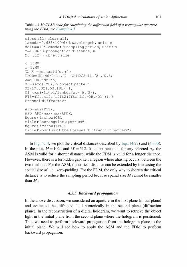
In Fig. 4.14, we plot the critical distances described by Eqs. (4.27) and (4.33b).In the plot, M¼ 1024 and M0 ¼ 512. It is apparent that, for any selected Δx, theASM is valid for a shorter distance, while the FDM is valid for a longer distance.However, there is a forbidden gap, i.e., a region where aliasing occurs, between thetwo methods. For the ASM, the critical distance can be extended by increasing thespatial sizeM, i.e., zero-padding. For the FDM, the only way to shorten the criticaldistance is to reduce the sampling period because spatial size M cannot be smallerthan M0.

4.3.5 Backward propagation

In the above discussion, we considered an aperture in the first plane (initial plane)and evaluated the diffracted field numerically in the second plane (diffractionplane). In the reconstruction of a digital hologram, we want to retrieve the objectlight in the initial plane from the second plane where the hologram is positioned.Thus we need to perform backward propagation from the hologram plane to theinitial plane. We will see how to apply the ASM and the FDM to performbackward propagation.

Table 4.4 MATLAB code for calculating the diffraction field of a rectangular apertureusing the FDM, see Example 4.5

close all; clear all;lambda¼0.633*10 -̂6; % wavelength, unit: mdelta¼10*lambda; % sampling period, unit: mz¼0.06; % propagation distance; mM0¼512; % object size

c¼1:M0;r¼1:M0;[C, R]¼meshgrid(c, r);THOR¼((R-M0/2-1). 2̂þ(C-M0/2-1). 2̂). 0̂.5;A¼THOR.*delta;OB¼zeros(M0); % object patternOB(193:321,53:181)¼1;Q1¼exp(-1i*pi/lambda/z.*(A. 2̂));FTS¼fftshift(ifft2(fftshift(OB.*Q1)));%Fresnel diffraction

AFD¼abs(FTS);AFD¼AFD/max(max(AFD));figure; imshow(OB);title(’Rectangular aperture’)figure; imshow(AFD);title(’Modulus of the Fresnel diffraction pattern’)


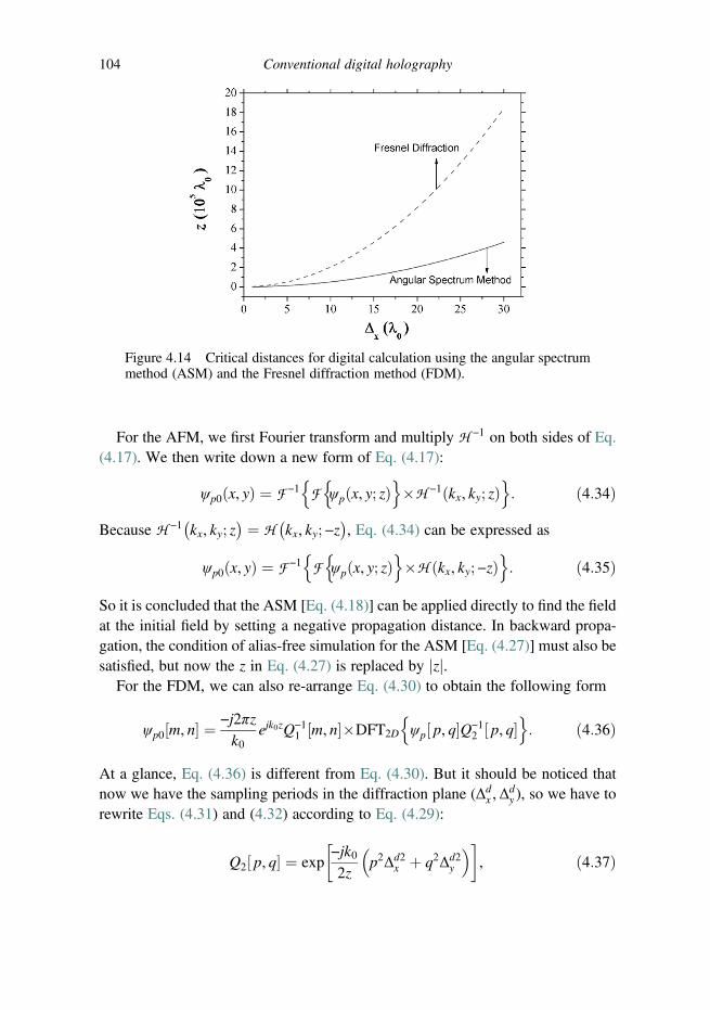
For the AFM, we first Fourier transform and multiply H −1 on both sides of Eq.(4.17). We then write down a new form of Eq. (4.17):

ψp0ðx, yÞ ¼ F −1 F ψp x, y; zð Þn o

�H −1ðkx, ky; zÞn o

: ð4:34Þ

Because H −1 kx, ky; z� ¼ H kx, ky; −z

� , Eq. (4.34) can be expressed as

ψp0ðx, yÞ ¼ F −1 F ψp x, y; zð Þn o

�H ðkx, ky;−zÞn o

: ð4:35Þ

So it is concluded that the ASM [Eq. (4.18)] can be applied directly to find the fieldat the initial field by setting a negative propagation distance. In backward propa-gation, the condition of alias-free simulation for the ASM [Eq. (4.27)] must also besatisfied, but now the z in Eq. (4.27) is replaced by jzj.

For the FDM, we can also re-arrange Eq. (4.30) to obtain the following form

ψp0 m, n½ � ¼ −j2πzk0

ejk0zQ−11 m, n½ ��DFT2D ψp½ p, q�Q−1

2 ½ p, q�n o

: ð4:36Þ

At a glance, Eq. (4.36) is different from Eq. (4.30). But it should be noticed thatnow we have the sampling periods in the diffraction plane (Δd

x ,Δdy ), so we have to

rewrite Eqs. (4.31) and (4.32) according to Eq. (4.29):

Q2 p, q½ � ¼ exp−jk02z

p2Δd2x þ q2Δd2

y

� � �, ð4:37Þ

Figure 4.14 Critical distances for digital calculation using the angular spectrummethod (ASM) and the Fresnel diffraction method (FDM).


Q1½m, n� ¼ exp −jπλzm

MΔdx

!2

þ n

NΔdy

!224

35

8<:

9=;: ð4:38Þ

Consequently, Eq. (4.36) can be re-expressed as

ψp0 m, n½ � ¼ −j2πzk0

ejk0zQ2ð−zÞ m, n½ ��DFT2D ψp½p, q�Q1ð−zÞ½ p, q�n o

, ð4:39Þ

where Q2ð−zÞ ¼ Q−12ðzÞ and Q1ð−zÞ ¼ Q−1

1ðzÞ. In comparison with Eq. (4.30) andEq. (4.39), we conclude that the FDM [Eq. (4.30)] can also be applied to findthe intensity distribution in the initial plane. Neglecting the proportionalityconstant, the only difference is that in Eq. (4.30) IDFT2D{•} is involved whilein Eq. (4.39) DFT2D{•} is involved. So in backward propagation using theFDM [Eq. (4.30)] with a negative propagation distance, the calculated intensitydistribution will be inverted. One can invert the calculation result manually toshow the correct diffraction pattern.

4.4 Optical recording of digital holograms

The recording of a digital hologram is simpler than recording on a holographicfilm. First, the sensitivity of a digital imager is several orders of magnitude higherthan that of holographic film. Thus the problem of vibration during holographicrecording in conventional holography is not serious in digital holography. Second,the response of a digital imager is linear so that problems of non-linearity associ-ated with the film [9, 10] are negligible in digital holography. However, the mainissue with digital holographic recording is that the maximum fringe frequency inthe hologram should be smaller than the Nyquist frequency associated with theimager. Otherwise, the fringes are under-sampled and aliasing occurs.

4.4.1 Recording geometry

On-axis Fresnel holography

The bandwidth of the holographic fringes depends on the form of the referencelight, the recording geometry, and the type of recording method. Here we takeon-axis Fresnel holography with a plane wave reference wave as an example.Assume that the CCD contains M�M pixels, so its size is MΔxCCD�MΔxCCD .The size of the object target is D and it is centered at the optical axis, as shownin Fig. 4.15. The distance between the object and the CCD sensor is z, and theplane wave reference wave is coupled to the object light via a beamsplitter (BS) ora half-silvered mirror. In the CCD plane, each object point together with the

4.4 Optical recording of digital holograms 105

reference wave forms a FZP. We can easily see that the ray of the object lightemitting from its lower edge to the upper edge of the CCD sensor (dashed linein Fig. 4.15) forms a maximum angle with respect to the z-axis (rays formingdiagonal connections between the object and the CCD sensor are ignored).Thus, the maximum transverse propagation distance of such a ray isðD=2þ MΔxCCDð Þ=2Þ, and the corresponding maximum local fringe frequency[see Eq. (2.5)] is ðDþMΔxCCDÞ=2λz. To avoid under-sampling of the holographicfringes, the maximum local fringe frequency must be smaller than the Nyquistfrequency [see Eq. (4.5)] associated with the CCD, that is

ðDþMΔxCCDÞ2λz

� 12ΔxCCD

, ð4:40aÞ

or

z � ΔxCCD

λDþMΔxCCDð Þ: ð4:40bÞ

Therefore, there is a minimum distance between the object and the CCD imagerif aliasing is to be avoided

Off-axis Fresnel holography

The above analysis can be extended to a generalized case in which the objectpattern is not located at the center of the optical axis, and the plane wave referencewave is tilted, as shown in Fig. 4.16. The minimum distance is found to be

z � ΔxCCD Dþ 2δþMΔxCCDð Þðλ−2 sinθΔxCCDÞ

, ð4:41Þ

where δ is the transverse shift of the object from its center, and θ is the offset angleof the reference wave. Note that in Eqs. (4.40) and (4.41), the zeroth-order beam

Figure 4.15 Setup of on-axis Fresnel holography.


and the twin image are not considered. In other words, the condition in Eq. (4.41)ensures only that the hologram is well sampled and it does not guarantee that allthese beams are separated in the reconstruction plane. We will discuss this aspectin Section 4.4.2.

Fourier holography

Figure 4.17 depicts the geometry of Fourier holography. Now the object and theCCD are at the front focal plane and the back focal plane of the Fourier lens,respectively. In this geometry, an off-axis object point produces a tilted plane waveon the CCD plane, resulting in a uniform sinusoidal fringe with the plane wavereference light [also see Fig. 3.7(a)]. However, the finest fringe is contributed bythe point source emitting at the margin of the object at x¼D/2. The finest fringeon the CCD plane therefore is given by [see Eq. (3.12)]

1þ e jkxD=22 ¼ 2þ 2 cos π

xD

λf

� �, ð4:42Þ

where kx¼ 2πx/λf. Thus to resolve the finest fringe, the local fringe frequency mustbe smaller than the Nyquist frequency associated with the CCD, that is,

Figure 4.17 Setup of Fourier holography.

Figure 4.16 Setup of off-axis Fresnel holography.


D

2λf� 1

2ΔxCCD, ð4:43aÞ

or

D � λfΔxCCD

, ð4:43bÞ

where f is the focal length of the Fourier transform lens. Note that the Fourierhologram can be regarded as a recording of the spectrum with resolutionΔk ¼ 2πΔxCCD=λf . So the size of the reconstruction space can be evaluated to be2π=Δk ¼ λf =ΔxCCD , which is consistent with Eq. 4.43(b). So the resolution, or thesampling distance Δx, of the reconstructed image is given by

Δx ¼ λfMΔxCCD

, ð4:44Þ

where MΔxCCD is the width of the CCD imager. Again, the twin image and thezeroth-order light are not taken into account in the above analysis.

4.4.2 Removal of the twin image and the zeroth-order light

Fourier holography

Here we consider separating the zeroth-order light and the twin image fromthe reconstructed image in a Fourier hologram. The Fourier hologram is recon-structed by performing a single Fourier transform. The zeroth-order light islocated at the center of the reconstruction plane, and the real image (the 1st order)appears at the location of the original object. The twin image (the −1st order) isflipped and a complex conjugate duplicate of the real image [see Fig. 3.7(b)].Similar to the spectrum of the off-axis Fresnel hologram (Fig. 3.4), the sizes ofthe real image and the twin image are the same, while the size of the zeroth-orderbeam is twice that of the real image. Consequently, the size of the real imageshould be smaller than one fourth of the size of the reconstruction space to ensurethat all the diffracted orders are separated on the reconstruction plane. In otherwords, in taking the Fourier hologram, the real image size as well as the objectsize should be smaller than λf =4ΔxCCD , according to Eq. (4.43b), and the objectmust be far from the center of the optical axis to avoid crosstalk betweendifferent diffracted orders.

Off-axis Fresnel holography

A single digital hologram acquired by a CCD imager is an amplitude hologramcontaining the real image, the virtual image, and the zeroth-order beam. Similar


to optical holography, the three diffracted orders can be separated in the off-axisgeometry (Fig. 4.16). In Section 3.2, we showed that the offset angle of thereference light should be large enough to avoid the interference between the 1storder and the zeroth-order beam, i.e.,

2πλ

sinθ � 32B, ð4:45Þ

where B is the bandwidth of the 1st and −1st orders of light. On the other hand,the angle of the reference light cannot be too large. Otherwise, the 1st order will beunder-sampled. Thus another condition is given by

2πλ

sinθ þ B

2� 2π

2ΔxCCD: ð4:46Þ

The bandwidth of the object light, B, depends on the light upon the CCD with thelargest incident angle. Similar to the analysis of Eq. (4.40), the bandwidth can bedetermined to be

B ¼ 2πðDþMΔxCCDÞ

λz: ð4:47Þ

Combining Eqs. (4.45), (4.46), and (4.47), the offset angle of the reference light islimited to the range

sin −1 3ðDþMΔxCCDÞ2z

� �� θ � sin −1 λ

2ΔxCCD−ðDþMΔxCCDÞ

2z

� �: ð4:48Þ

In Eq. (4.48), the critical condition occurs as the equals sign is selected, giving

3ðDþMΔxCCDÞ2z

¼ λ2ΔxCCD

−ðDþMΔxCCDÞ

2z: ð4:49Þ

After some manipulations, we can find the critical distance

zc ¼ 4ΔxCCDðDþMΔxCCDÞλ

, ð4:50Þ

which is also the minimum distance for successful off-axis holography. By substi-tuting Eq. (4.50) into Eq. (4.48), we can also find the critical offset angle

θc ¼ sin −1 3λ8ΔxCCD

� �: ð4:51Þ


Equations (4.50) and (4.51) describe the optimized recording conditions foroff-axis digital holography.

Example 4.6: Recording an off-axis digital hologram

We assume that a CCD contains 1024� 1024 pixels with pixel pitch 8 μm. Thesize of the object to be recorded is 1 cm, and the wavelength is 0.633 μm. Calculatethe optimized conditions for recording an off-axis digital hologram.

We can easily find the critical distance and the critical offset angle accordingto Eq. (4.50) and Eq. (4.51),

zc ¼ 4ð8 μmÞð104 μmþ 1024�8 μmÞ0:633 μm

¼ 92 cm

and

θc ¼ sin −1 3�0:633 μm8�8 μm

� �¼ 1:7:

So the offset angle is 1.7 and the minimum distance between the object andthe CCD is 92 cm in order to avoid aliasing. It should be noted that accordingto Section 4.2, the resolution of the reconstructed image, using Eq. (4.50),now is

λzMΔxCCD

¼ 4ðDþMΔxCCDÞM

¼ 4ð104 μmþ 1024�8 μmÞ1024

¼ 71μm,

which is much larger than the pixel pitch of the CCD. If a larger offset angle aswell as a larger propagation distance are selected, the resolution of the recon-structed image will be sacrificed further.

According to the above analysis, we can see that off-axis Fresnel holographyis not a satisfactory method for acquiring digital holograms because most ofthe bandwidth of the imager is wasted. In Fourier holography, the bandwidth ofthe reconstructed real image only depends on the size of the imager. However, theobject size is limited to one fourth of the field of view. Phase-shifting holography(PSH) is an efficient technique to alleviate the problem of the twin image and thezeroth-order light without sacrificing the bandwidth or the field of view. In PSH,several digital holograms with different phase shifts between them are used toretrieve the complex field of the object light. The details of PSH will be discussedin Section 5.1.


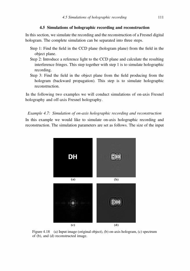
4.5 Simulations of holographic recording and reconstruction

In this section, we simulate the recording and the reconstruction of a Fresnel digitalhologram. The complete simulation can be separated into three steps.

Step 1: Find the field in the CCD plane (hologram plane) from the field in theobject plane.

Step 2: Introduce a reference light to the CCD plane and calculate the resultinginterference fringes. This step together with step 1 is to simulate holographicrecording.

Step 3: Find the field in the object plane from the field producing from thehologram (backward propagation). This step is to simulate holographicreconstruction.

In the following two examples we will conduct simulations of on-axis Fresnelholography and off-axis Fresnel holography.

Example 4.7: Simulation of on-axis holographic recording and reconstruction

In this example we would like to simulate on-axis holographic recording andreconstruction. The simulation parameters are set as follows. The size of the input

Figure 4.18 (a) Input image (original object), (b) on-axis hologram, (c) spectrumof (b), and (d) reconstructed image.

4.5 Simulations of holographic recording 111

Table 4.5 MATLAB code for simulation of on-axis holographic recording andreconstruction, see Example 4.7

clear all; close all;I¼imread(’DH256.bmp’,’bmp’); % 256�256 pixels, 8bit imageI¼double(I);

% parameter setupM¼256;deltax¼0.001; % pixel pitch 0.001 cm (10 um)w¼633*10 -̂8; % wavelength 633 nmz¼25; % 25 cm, propagation distance

%Step 1: simulation of propagation using the ASMr¼1:M;c¼1:M;[C, R]¼meshgrid(c, r);A0¼fftshift(ifft2(fftshift(I)));deltaf¼1/M/deltax;p¼exp(-2i*pi*z.*((1/w) 2̂-((R-M/2- 1).*deltaf). 2̂-. . .

((C-M/2-1).*deltaf). 2̂). 0̂.5);Az¼A0.*p;EO¼fftshift(fft2(fftshift(Az)));

%Step 2: interference at the hologram planeAV¼4*(min(min(abs(EO)))þmax(max(abs(EO))));% amplitude of reference light% the visibility can be controlled by modifying the amplitudeIH¼(EOþAV).*conj(EOþAV);figure; imshow(I);title(’Original object’)axis off

figure; imshow(mat2gray(IH));title(’Hologram’)axis off

SP¼abs(fftshift(ifft2(fftshift(IH))));figure; imshow(500.*mat2gray(SP));title(’Hologram spectrum’)axis off

%Step 3: reconstructionA1¼fftshift(ifft2(fftshift(IH)));Az1¼A1.*conj(p);EI¼fftshift(fft2(fftshift(Az1)));EI¼mat2gray(EI.*conj(EI));figure; imshow(EI);title(’Reconstructed image’)axis off


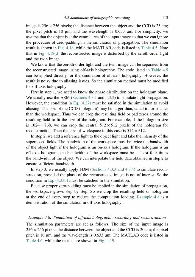
image is 256� 256 pixels; the distance between the object and the CCD is 25 cm;the pixel pitch is 10 μm, and the wavelength is 0.633 μm. For simplicity, weassume that the object is at the central area of the input image so that we can ignorethe procedure of zero-padding in the simulation of propagation. The simulationresult is shown in Fig. 4.18, while the MATLAB code is listed in Table 4.5. Notethat in Fig. 4.18(d) the reconstructed image is disturbed by the zeroth-order lightand the twin image.

We know that the zeroth-order light and the twin image can be separated fromthe reconstructed image using off-axis holography. The code listed in Table 4.5can be applied directly for the simulation of off-axis holography. However, theresult is noisy due to aliasing issues. So the simulation method must be modifiedfor off-axis holography.

First in step 1, we need to know the phase distribution on the hologram plane.We usually use the ASM (Sections 4.3.1 and 4.3.2) to simulate light propagation.However, the condition in Eq. (4.27) must be satisfied in the simulation to avoidaliasing. The size of the CCD (hologram) may be larger than, equal to, or smallerthan the workspace. Thus we can crop the resulting field or pad zeros around theresulting field to fit the size of the hologram. For example, if the hologram sizeis 1024� 768, we can crop the central 512� 512 pixels of the hologram forreconstruction. Then the size of workspace in this case is 512� 512.

In step 2, we add a reference light to the object light and take the intensity of thesuperposed fields. The bandwidth of the workspace must be twice the bandwidthof the object light if the hologram is an on-axis hologram. If the hologram is anoff-axis hologram, the bandwidth of the workspace must be at least four timesthe bandwidth of the object. We can interpolate the field data obtained in step 2 toensure sufficient bandwidth.

In step 3, we usually apply FDM (Sections 4.3.3 and 4.3.4) to simulate recon-struction, provided the phase of the reconstructed image is not of interest. So thecondition in Eq. (4.33b) must be satisfied in the simulation.

Because proper zero-padding must be applied in the simulation of propagation,the workspace grows step by step. So we crop the resulting field or hologramat the end of every step to reduce the computation loading. Example 4.8 is ademonstration of the simulation in off-axis holography.

Example 4.8: Simulation of off-axis holographic recording and reconstruction

The simulation parameters are set as follows. The size of the input image is256� 256 pixels; the distance between the object and the CCD is 20 cm; the pixelpitch is 10 μm, and the wavelength is 0.633 μm. The MATLAB code is listed inTable 4.6, while the results are shown in Fig. 4.19.

4.5 Simulations of holographic recording 113

Table 4.6 MATLAB code for simulation of off-axis holographic recording andreconstruction, see Example 4.8

clear all; close all;%% Reading input bitmap fileI0¼imread(’DH256.bmp’,’bmp’); % 256�256 pixels, 8bit imageI0¼double(I0);

% parameter setupM¼256;deltax¼0.001; % pixel pitch 0.001 cm (10 um)w¼633*10 -̂8; % wavelength 633 nmz¼20; % z¼M*deltax 2̂/w; % propagation distance

% Step 1: simulation of propagationr¼1:5*M;c¼1:5*M;[C, R]¼meshgrid(c, r);I¼zeros(5*M);I(513:768,513:768)¼I0;A0¼fftshift(ifft2(fftshift(I)));deltaf¼1/5/M/deltax;p¼exp(-2i*pi*z.*((1/w) 2̂-((R-641).*deltaf). 2̂-. . .

((C-641).*deltaf). 2̂). 0̂.5);Az¼A0.*p;EO¼fftshift(fft2(fftshift(Az)));EO¼EO(513:768,513:768); % reduce diffraction-plane size

% Step 2: interference at the hologram plane% zero-padding in the spectrum domainAz¼fftshift(ifft2(fftshift(EO)));Az2¼zeros(4*M);Az2(385:640,385:640)¼Az;EOf¼fftshift(fft2(fftshift(Az2)));

AV¼(min(min(abs(EOf)))þmax(max(abs(EOf))))/2;angle¼0.3; % reference beam angle; degreer2¼1:4*M;c2¼1:4*M;[C2, R2]¼meshgrid(c2, r2);

Ref¼AV*exp(1i*2*pi*sind(angle)*deltax/4.*. . .(R2-2*M-1)/wþ1i*2*pi*sind(angle)*deltax/4.*. . .(C2-2*M-1)/w);IH¼(EOfþRef).*conj(EOfþRef);IH¼IH(257:768,257:768); % reduce the hologram size

figure; imshow(mat2gray(IH));title(’Hologram’)


Table 4.6 (cont.)

axis offSP¼fftshift(ifft2(fftshift(IH)));figure; imshow(50.*mat2gray(abs(SP)));title(’Hologram spectrum’)axis off

% Step 3: reconstruction (Fresnel diffraction)r3¼1:2*M;c3¼1:2*M;[C3, R3]¼meshgrid(c3, r3);THOR¼((R3-M-1). 2̂þ(C3-M-1). 2̂). 0̂.5;A¼THOR.*deltax/4;QP¼exp(1i*pi/w/z.*(A. 2̂));FTS¼fftshift(fft2(fftshift(IH.*QP)));I2¼FTS.*conj(FTS);figure; imshow(5.*mat2gray(I2));title(’Reconstructed image’)axis off

Figure 4.19 (a) Off-axis hologram, (b) spectrum of (a), and (c) reconstructedimage.

Problems 115

Problems

4.1 Following Example 4.3, calculate and plot the spectrum of a shifted rectangu-lar function, i.e., the rectangular function is not centered at the axis origin.

4.2 Perform and plot the FFT of a rectangular function using MATLAB. Also plotthe spectrum of the rectangular function using the result from Table 1.1.Compare the two plots and if you are performing the calculations correctly,you will see that there is a little difference between the two curves.

4.3 Show that the spectrum of the sampled signal f ðxÞ�X∞

n¼−∞δðx−nΔxÞ is

periodic in the spectrum domain as follows:

F f ðxÞ�X∞n¼−∞

δðx−nΔxÞ( )

¼ 2πf sX∞n¼−∞

Fðkx−2πf snÞ,

where fs¼ 1/Δx.4.4 Using the Fresnel diffraction method (FDM) to calculate the diffracted field,

and if the sampling period on the object plane along the x-axis is Δx with totalM samples, and the sampling period along the y-axis is Δy with totalN samples, show that at the diffraction plane with the number of samplesbeing the same, the sampling periods (Δd

x ,Δdy ) change according to the

following relationships:

Δdx ¼

λzMΔx

, Δdy ¼

λzNΔy

,

as given by Eq. (4.29).4.5 Assume that an on-axis hologram is acquired according to the well-sampling

condition in Eq. (4.40), i.e., the distance between the object and the CCD is

z ¼ ΔxCCD

λDþMΔxCCDð Þ:

Ignore the problem of the zeroth-order light and the twin image. Calculatethe resolution of the reconstructed image.

4.6 In off-axis Fresnel holography and for aliasing-free calculations, show that theminimum distance of the object from the CCD is

z � ΔxCCD Dþ 2δþMΔxCCDð Þðλ−2 sin θΔxCCDÞ

, ð4:41Þ

where D is the size of the object, δ is the transverse shift of the object from thecenter of the object plane, and θ is the offset angle of the reference wave asshown in Fig. 4.16.


References

1. D. H. Seib, Carrier diffusion degradation of modulation transfer function in chargecoupled imagers, IEEE Transactions on Electron Devices 21, 210–217 (1974).

2. S. G. Chamberlain, and D. H. Harper, MTF simulation including transmittance effectsand experimental results of charge-coupled imagers, IEEE Transactions on ElectronDevices 25, 145–154 (1978).

3. J. C. Feltz, and M. A. Karim, Modulation transfer function of charge-coupled devices,Applied Optics 29, 717–722 (1990).

4. E. G. Stevens, A unified model of carrier diffusion and sampling aperture effectson MTF in solid-state image sensors, IEEE Transactions on Electron Devices 39,2621–2623 (1992).

5. M. Marchywka, and D. G. Socker, Modulation transfer function measurement tech-nique for small-pixel detectors, Applied Optics 31, 7198–7213 (1992).

6. A. M. Pozo, and M. Rubiño, Comparative analysis of techniques for measuring themodulation transfer functions of charge-coupled devices based on the generation oflaser speckle, Applied Optics 44, 1543–1547 (2005).

7. A. M. Pozo, A. Ferrero, M. Ubiño, J. Campos, and A. Pons, Improvements fordetermining the modulation transfer function of charge-coupled devices by the specklemethod, Optics Express 14, 5928–5936 (2006).

8. J.-P. Liu, Controlling the aliasing by zero-padding in the digital calculation of thescalar diffraction, Journal of the Optical Society of America A 29, 1956–1964 (2012).

9. A. A. Friesem, and J. S. Zelenka, Effects of film nonlinearities in holography, AppliedOptics 6, 1755–1759 (1967).

10. O. Bryngdail, and A. Lohmann, Nonlinear effects in holography, Journal of theOptical Society of America 58, 1325–1330 (1968).

References 117

5

Digital holography: special techniques

In Chapter 4, we introduced conventional digital holography, describing on-axisFresnel holograms, off-axis Fresnel holograms, and Fourier holograms. In thischapter we will introduce some important techniques in digital holography, includ-ing phase-shifting digital holography, low-coherence digital holography, tomo-graphic holography, and optical scanning holography.

5.1 Phase-shifting digital holography

In optical holography, the off-axis geometry is an effective configuration forseparating the zeroth-order light and the twin image. However, as indicated inSection 4.4, it is difficult to record a high-quality off-axis Fresnel hologrambecause of the limitation of the narrow bandwidth of the CCD. However, if theon-axis geometry is employed, it is necessary to eliminate the zeroth-order lightand the twin image. Among the various available techniques, phase-shiftingholography (PSH) is the most widely used technique to achieve this goal [1–3].Figure 5.1 depicts a typical setup for PSH. The setup is nearly the same as thatfor conventional on-axis digital holography. The only difference is that one ofthe mirrors is mounted on a piezoelectric transducer (PZT) in PSH so that theoptical path difference between the object light and the reference light can beadjusted. The phase difference should be precisely controlled through the PZT.Besides the use of a PZT, other phase-shifting mechanisms include the use ofan electro-optic modulator [4], an acousto-optic modulator [5], a wave plate[6], and a tilted slab [7]. Phase shifting can be applied to any holographicrecording geometry: on-axis holography, off-axis holography [8], or Gaborholography [9].

In PSH, we need to take multiple holograms corresponding to the various phasedifferences between the object light and the reference light. In general, the holo-gram can be expressed as

118

Iδ ¼ jψ0 þ ψrexp −jδð Þj2¼ jψ0j2 þ jψrj2 þ ψ0ψ

�rexp jδð Þ þ ψ�

0ψrexp −jδð Þ, ð5:1Þwhere ψ0 and ψr stand for the complex amplitude of the object light and thereference light, respectively; δ stands for the phase induced by the phase shifter.Multiple holograms are acquired sequentially and, upon complete acquisition, thecomplex amplitude of the object light can be derived from the holograms.

5.1.1 Four-step phase-shifting holography

In four-step PSH, four holograms are acquired sequentially. The phase differencesfor the four holograms are δ ¼ 0, δ ¼ π/2, δ ¼ π, and δ ¼ 3π/2. Therefore,according to Eq. (5.1), the four holograms can be expressed as

I0 ¼ jψ0j2 þ jψrj2 þ ψ0ψ�r þ ψ�

0ψr,

Iπ=2 ¼ jψ0j2 þ jψrj2 þ jψ0ψ�r − jψ

�0ψr,

Iπ ¼ jψ0j2 þ jψrj2 −ψ0ψ�r −ψ

�0ψr,

I3π=2 ¼ jψ0j2 þ jψrj2 − jψ0ψ�r þ jψ�

0ψr:

First, we can remove the zeroth-order light, jψ0j2 þ jψrj2, by the followingsubtractions:

I0−Iπ ¼ 2ψ0ψ�r þ 2ψ�

0ψr ð5:2aÞIπ=2−I3π=2 ¼ 2jψ0ψ

�r −2jψ

�0ψr: ð5:2bÞ

Then, the conjugate term of ψ0, i.e., ψ�0, can be removed by an additional subtrac-

tion as follows:

Figure 5.1 Schematic of phase-shifting holography. BE beam expander; BSbeam splitter.

5.1 Phase-shifting digital holography 119

I0 − Iπð Þ− jðIπ=2 − I3π=2Þ ¼ 4ψ0ψ�r : ð5:3Þ

Finally, the complex amplitude of the object light is given by

ψ0 ¼I0 − Iπð Þ− jðIπ=2 − I3π=2Þ

4ψ�r

: ð5:4Þ

In the field of digital holography, the complex amplitude of the object light issometimes referred to as the complex hologram because we can retrieve theamplitude distribution of the object light in the object plane from ψ0 by performingdigital back-propagation. Note that in Eq. (5.4) the complex amplitude of thereference light must be known in order to calculate ψ0. Otherwise, only the productof ψ0 and ψ�

r is retrieved. Usually, the reference light is a plane wave or a sphericalwave and therefore its phase is known without any measurement.

5.1.2 Three-step phase-shifting holography

Four-step PSH can be simplified to three-step PSH, in which only three hologramsare involved. The phase differences for the three holograms are δ ¼ 0, δ ¼ π/2, andδ¼ π. After some mathematical manipulation, the complex amplitude of the objectcan be found to be

ψ0 ¼ð1þ jÞ I0 − Iπ=2

� �þ ð j−1ÞðIπ − Iπ=2Þ4ψ�

r

: ð5:5Þ

5.1.3 Two-step phase-shifting holography

Could the steps of phase shifting be reduced further? The answer is affirmative,and there is two-step PSH. Suppose that two holograms with a zero phase shift anda π/2 phase shift are obtained [see Eq. (5.1)]. In addition, the intensities of theobject light, jψ0j2, and the reference light, jψrj2, are measured. We can remove thezeroth-order light from the two holograms as follows:

I0 − jψ0j2 − jψrj2 ¼ ψ0ψ�r þ ψ�

0ψr ð5:6aÞIπ=2 − jψ0j2 − jψrj2 ¼ jψ0ψ

�r − jψ

�0ψr: ð5:6bÞ

As a result, the complex amplitude of the object light is found to be

ψ0 ¼I0 − jψ0j2 − jψrj2

� �− j Iπ=2 − jψ0j2 − jψrj2� �

2ψ�r

: ð5:7Þ

Because in this case only two holograms with a zero phase shift and a π/2 phaseshift are needed, the technique is also called quadrature-phase shifting holography

120 Digital holography: special techniques

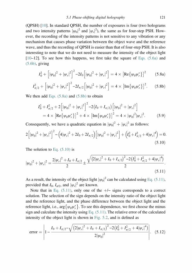
(QPSH) [10]. In standard QPSH, the number of exposures is four (two hologramsand two intensity patterns jψ0j2 and jψrj2), the same as for four-step PSH. How-ever, the recording of the intensity patterns is not sensitive to any vibration or anymechanism that causes phase variation between the object wave and the referencewave, and thus the recording of QPSH is easier than that of four-step PSH. It is alsointeresting to note that we do not need to measure the intensity of the object light[10–12]. To see how this happens, we first take the square of Eqs. (5.6a) and(5.6b), giving

I20 þ jψ0j2 þ jψrj2h i2

−2I0 jψ0j2 þ jψrj2h i

¼ 4� Re ψ0ψ�r

� �� 2 ð5:8aÞ

I2π=2 þ jψ0j2 þ jψrj2h i2

−2Iπ=2 jψ0j2 þ jψrj2h i

¼ 4� Im ψ0ψ�r

� �� 2: ð5:8bÞ

We then add Eqs. (5.8a) and (5.8b) to obtain

I20 þ I2π=2 þ 2 jψ0j2 þ jψrj2h i2

−2 I0 þ Iπ=2� � jψ0j2 þ jψrj2

h i¼ 4� Re ψ0ψ

�r

� �� 2 þ 4� Im ψ0ψ�r

� �� 2 ¼ 4� jψ0j2jψrj2: ð5:9ÞConsequently, we have a quadratic equation in jψ0j2 þ jψrj2 as follows:

2 jψ0j2þjψrj2h i2

− 4jψrj2þ2I0þ2Iπ=2� �

jψ0j2þjψrj2h i

þ I20þ I2π=2þ4jψrj4� �

¼ 0:

ð5:10ÞThe solution to Eq. (5.10) is

jψ0j2 þ jψrj2 ¼2jψrj2 þ I0 þ Iπ=2

2�

ffiffiffiffiffiffiffiffiffiffiffiffiffiffiffiffiffiffiffiffiffiffiffiffiffiffiffiffiffiffiffiffiffiffiffiffiffiffiffiffiffiffiffiffiffiffiffiffiffiffiffiffiffiffiffiffiffiffiffiffiffiffiffiffiffiffiffiffiffiffiffiffiffiffiffiffiffiffiffiffiffiffi�2jψrj2 þ I0 þ Iπ=2

�2−2

�I20 þ I2π=2 þ 4jψrj4

�q2

:

ð5:11ÞAs a result, the intensity of the object light jψ0j2 can be calculated using Eq. (5.11),provided that I0, Iπ/2, and jψrj2 are known.

Note that in Eq. (5.11), only one of the þ/− signs corresponds to a correctsolution. The selection of the sign depends on the intensity ratio of the object lightand the reference light, and the phase difference between the object light and thereference light, i.e., arg ψ0ψ

�r

� �. To see this dependence, we first choose the minus

sign and calculate the intensity using Eq. (5.11). The relative error of the calculatedintensity of the object light is shown in Fig. 5.2, and is defined as

error ¼ 1−I0 þ Iπ=2−

ffiffiffiffiffiffiffiffiffiffiffiffiffiffiffiffiffiffiffiffiffiffiffiffiffiffiffiffiffiffiffiffiffiffiffiffiffiffiffiffiffiffiffiffiffiffiffiffiffiffiffiffiffiffiffiffiffiffiffiffiffiffiffiffiffiffiffiffiffiffiffiffiffiffiffiffiffiffiffiffiffiffiffiffiffi�2jψrj2 þ I0 þ Iπ=2

�2−2

�I20 þ I2π=2 þ 4jψrj4

�q2jψ0j2

��: ð5:12Þ


In Fig. 5.2, the gray-level represents the amount of error. We can see that the errorin the range of 2π is small only when the relative intensity, defined as jψrj2/jψ0j2, islarger than 2. Accordingly, to ensure that the calculated intensity of the object lightat any pixel is correct, the intensity of the reference light must be at least two timeslarger than the maximum intensity of the object light. This demand limits thedynamic range of the acquired digital holograms, and thus limits the signal-to-noise ratio of the reconstructed images. When the plus sign in Eq. (5.11) is chosen,results indicate that not only the relative intensity but also arg ψ0ψ

�r

� �must be

limited to a small range to ensure a small error. So the minus sign in Eq. (5.11) isalways selected.

5.1.4 Phase step and phase error

In the above analysis, the phase step is always π/2 for four-step PSH, three-stepPSH, and two-step PSH. However, the complex object field can be reconstructedfor any phase step ranging between 0 and π. Here we take two-step PSH as anexample. For an arbitrary phase step δ, the two holograms acquired are

I1 ¼ jψ0j2 þ jψrj2 þ ψ0ψ�r þ ψ�

0ψr ð5:13aÞI2 ¼ jψ0j2 þ jψrj2 þ ψ0ψ

�r exp −jδð Þ þ ψ�

0ψr exp jδð Þ: ð5:13bÞ

Figure 5.2 Error of the calculated intensity of the object light as a function ofboth the phase difference, arg ψ0ψ

�r

� �, and the relative intensity, jψrj2/jψ0j2. See

Table 5.1 for the MATLAB code.


Equations (5.13a) and (5.13b) can be rearranged to become

ψoψ�r þ ψ�

oψr ¼ I1 − jψoj2 − jψrj2, ð5:14aÞψoψ

�rexp −jδð Þ þ ψ�

oψr exp jδð Þ ¼ I2 − jψoj2 − jψrj2: ð5:14bÞWe now subtract Eq. (5.14b) from Eq. (5.14a) after multiplying Eq. (5.14a) by exp(jδ). The result of the subtraction is

2ψ0ψ�r sin δð Þ ¼ I1 − jψ0j2 − jψrj2

� �exp jδð Þ− I2 − jψ0j2 − jψrj2

� �: ð5:15Þ

Consequently, the complex amplitude of the object wave can be retrieved by

ψ0 ¼I1 − jψ0j2 − jψrj2

� �exp jδð Þ− I2 − jψ0j2 − jψrj2

� �2ψ�

r sin δð Þ : ð5:16Þ

According to Eq. (5.16), the phase step δ can be arbitrary in the range 0 < δ < πor −π < δ < 0.

Equation (5.16) shows that the phase step can be arbitrary in a wide range.However, in practice, tolerance of the phase step in phase-shifting holography is aproblem. Tolerance may be due to the inaccuracy of the phase shifter, air turbu-lence, or vibration. It can be easily shown that for a fixed tolerance of the phasestep, the minimum error of the retrieved object field can be obtained when the π/2(or −π/2) phase step is applied.

Table 5.1 MATLAB code for calculating the error of QPSH, see Fig. 5.2

clear all; close all;ii¼logspace(-1,1,1024);theta¼linspace(0,2,1024);[I,T]¼meshgrid(ii,theta);

I1¼1þIþ2*(I.^0.5).*cos(T*pi);I2¼1þIþ2*(I.^0.5).*sin(T*pi);D¼8*I.*I2-(I1-I2-2*I).^2;

Io¼(I1þI2-D.^0.5)./2;err¼abs(Io-1);

figure; mesh(I,T,err);view(2)set(gca, ‘XScale’, ‘log’) ;xlabel(‘Relative Intensity of the reference light’);ylabel(‘Phase difference (\pi radian)’);colorbaraxis tight


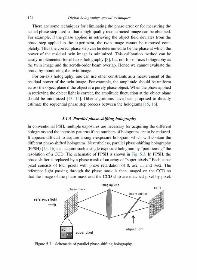
There are some techniques for eliminating the phase error or for measuring theactual phase step used so that a high-quality reconstructed image can be obtained.For example, if the phase applied in retrieving the object field deviates from thephase step applied in the experiment, the twin image cannot be removed com-pletely. Thus the correct phase step can be determined to be the phase at which thepower of the residual twin image is minimized. This calibration method can beeasily implemented for off-axis holography [8], but not for on-axis holography asthe twin image and the zeroth-order beam overlap. Hence we cannot evaluate thephase by monitoring the twin image.

For on-axis holography, one can use other constraints as a measurement of theresidual power of the twin image. For example, the amplitude should be uniformacross the object plane if the object is a purely phase object. When the phase appliedin retrieving the object light is correct, the amplitude fluctuation at the object planeshould be minimized [13, 14]. Other algorithms have been proposed to directlyestimate the sequential phase step process between the holograms [15, 16].

5.1.5 Parallel phase-shifting holography

In conventional PSH, multiple exposures are necessary for acquiring the differentholograms and the intensity patterns if the numbers of holograms are to be reduced.It appears difficult to acquire a single-exposure hologram which will contain thedifferent phase-shifted holograms. Nevertheless, parallel phase-shifting holography(PPSH) [15, 16] can acquire such a single-exposure hologram by “partitioning” theresolution of a CCD. The schematic of PPSH is shown in Fig. 5.3. In PPSH, thephase shifter is replaced by a phase mask of an array of “super pixels.” Each superpixel consists of four pixels with phase retardation of 0, π/2, π, and 3π/2. Thereference light passing through the phase mask is then imaged on the CCD sothat the image of the phase mask and the CCD chip are matched pixel by pixel.

Figure 5.3 Schematic of parallel phase-shifting holography.


In addition, the object light is also directed to the CCD by a beam splitter. As aresult, interferences on the four pixels of a super pixel correspond to four differentphase steps. Subsequently, we can calculate the complex amplitude of the objectwave using Eq. (5.4). The pixel size of the retrieved object light thus has the samesize as a super pixel, but is four times larger than the pixel size of the CCD.

The pixel-by-pixel imaging in Fig. 5.3 demands a high-precision alignment andis sensitive to environmental interference. An improvement is made by attachingthe phase mask directly against the CCD chip [17–19]. Alternatively, a randomphase mask can be used instead of a deterministic phase mask [20]. However,several pre-measurements must be performed in order to calibrate the phase of thereference light among super pixels.

Example 5.1: Simulation of four-step PSH

In this example we simulate the recording and reconstruction of four-step phase-shifting holography (PSH). Since PSH can be conducted using the geometry of on-axis holography, we adopt the simulation setup of on-axis holography (see Example4.7). The only difference is that we perform the recording four times, correspondingto the phase shifts 0, π/2, π, and 3π/2. The four holograms are shown in Fig. 5.4. Asthe holograms are recorded, we can find the complex holograms using Eq. (5.4) forfour-step PSH. The complex hologram can be reconstructed using standard back-ward propagation. The reconstructed image of the complex hologram is shown in

Figure 5.4 Four holograms for (a) δ¼ 0, (b) δ¼ π/2, (c) δ¼ π, and (d) δ¼ 3π/2.


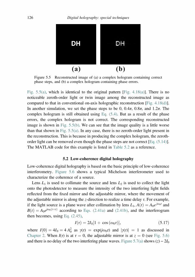
Fig. 5.5(a), which is identical to the original pattern [Fig. 4.18(a)]. There is nonoticeable zeroth-order light or twin image among the reconstructed image ascompared to that in conventional on-axis holographic reconstruction [Fig. 4.18(d)].In another simulation, we set the phase steps to be 0, 0.4π, 0.8π, and 1.2π. Thecomplex hologram is still obtained using Eq. (5.4). But as a result of the phaseerrors, the complex hologram is not correct. The corresponding reconstructedimage is shown in Fig. 5.5(b). We can see that the image quality is a little worsethan that shown in Fig. 5.5(a). In any case, there is no zeroth-order light present inthe reconstruction. This is because in producing the complex hologram, the zeroth-order light can be removed even though the phase steps are not correct [Eq. (5.14)].The MATLAB code for this example is listed in Table 5.2 as a reference.

5.2 Low-coherence digital holography

Low-coherence digital holography is based on the basic principle of low-coherenceinterferometry. Figure 5.6 shows a typical Michelson interferometer used tocharacterize the coherence of a source.

Lens L1 is used to collimate the source and lens L2 is used to collect the lightonto the photodetector to measure the intensity of the two interfering light fieldsreflected from the fixed mirror and the adjustable mirror, where the movement ofthe adjustable mirror is along the z-direction to realize a time delay τ. For example,if the light source is a plane wave after collimation by lens L1, A tð Þ ¼ A0e jω0t andB tð Þ ¼ A0ejω0ðtþτÞ according to Eqs. (2.41a) and (2.41b), and the interferogramthen becomes, using Eq. (2.45),

IðτÞ ¼ 2I0½1þ cos ω0τð Þ�, ð5:17Þwhere I 0ð Þ ¼ 4I0 ¼ 4 A2

0 as γ(τ) ¼ exp(jω0τ) and jγ(τ)j ¼ 1 as discussed inChapter 2. When I(τ) is at τ ¼ 0, the adjustable mirror is at z ¼ 0 (see Fig. 5.6)and there is no delay of the two interfering plane waves. Figure 5.7(a) shows (z) − 2I0

Figure 5.5 Reconstructed image of (a) a complex hologram containing correctphase steps, and (b) a complex hologram containing phase errors.


Table 5.2 MATLAB code for simulation of four-step PSH, see Example 5.1; the code isbased on simulation of an on-axis hologram (Example 4.7)

clear all; close all;I¼imread(‘DH256.bmp’,‘bmp’); % 256�256 pixels 8bit imageI¼double(I);

% parameter setupM¼256;deltax¼0.001; % pixel pitch 0.001 cm (10 um)w¼633*10^-8; % wavelength 633 nmz¼25; % 25 cm, propagation distancedelta¼pi/2; % phase step (change it to show part b)%Step 1: Simulation of propagation using the ASMr¼1:M;c¼1:M;[C, R]¼meshgrid(c, r);A0¼fftshift(ifft2(fftshift(I)));deltaf¼1/M/deltax;p¼exp(-2i*pi*z.*((1/w)^2-((R-M/2-1).*deltaf).^2-. . .

((C-M/2-1).*deltaf).^2).^0.5);Az¼A0.*p;EO¼fftshift(fft2(fftshift(Az)));

%Step 2: Interference at the hologram planeAV¼(min(min(abs(EO)))þmax(max(abs(EO))));% the amplitude of reference light

% Recording of Four phase-shifting hologramsI0¼(EOþAV).*conj(EOþAV);I1¼(EOþAV*exp(-1j*delta)).*conj(EOþAV*exp(-1j*delta));I2¼(EOþAV*exp(-2j*delta)).*conj(EOþAV*exp(-2j*delta));I3¼(EOþAV*exp(-3j*delta)).*conj(EOþAV*exp(-3j*delta));MAX¼max(max([I0, I1, I2, I3]));

figure(1); imshow(I);title(‘Original object’)axis offfigure(2)subplot(2,2,1)imshow(I0/MAX);axis offtitle(‘hologram 1’)subplot(2,2,2)imshow(I1/MAX);axis offtitle(‘hologram 2’)subplot(2,2,3)imshow(I2/MAX);axis offtitle(‘hologram 3’)

5.2 Low-coherence digital holography 127

versus τ, i.e., the bias has been subtracted from I(z) and only the intensity variationis plotted, for a plane wave source. In this case, we have complete coherence.

For a partially coherent source having a sinc-squared type power spectrum [seeEq. (2.63)], we have

IðτÞ ¼ 2I0 1þ Λττ0

� cos ω0τð Þ

� �ð5:18Þ

Table 5.2 (cont.)

subplot(2,2,4)imshow(I3/MAX);axis offtitle(‘hologram 4’)

%Step 3: ReconstructionCH¼(I0-I2)-1j*(I1-I3); % the complex hologram (4-step PSH)A1¼fftshift(ifft2(fftshift(CH)));Az1¼A1.*conj(p);EI¼fftshift(fft2(fftshift(Az1)));EI¼(EI.*conj(EI));EI¼EI/max(max(EI));figure(3);imshow(EI);title(‘Reconstructed image of 4-step PSH’)axis off

Figure 5.6 Michelson interferometer used to characterize the coherence of a source


according to Eq. (2.49). Figure 5.7(b) shows the intensity variation as a functionof τ, a phenomenon in which an interference pattern forms only when the opticalpath difference between the two incident fields is less than the coherence lengthof the light source, ℓc ¼ c • τ0. Low-coherence holography uses this phenomenonto allow for interference between the object wave and the reference wave.The thickness of the layer of the object that can be holographically recorded isabout half of the coherence length owing to the reflection setup. Since ℓc can bemade short by using an appropriate source, the thickness of the layer of a thickobject being recorded can be made small. The capability of imaging only a thinsection optically without any out-of-focus haze, i.e., noise coming from sectionsother than the section being imaged, is called optical sectioning [21–24]. Weshall adopt the holographic microscope investigated by Lin et al. [21] to illustratethe principle of low-coherence holography.

The principle of low-coherence holography is easily understood now thatwe have discussed low-coherence interferometry. The experimental setup of alow-coherence phase-shifting digital holographic microscope for measuring sec-tional images is shown in Fig. 5.8. It consists of a modified Michelson interfer-ometer with a PZT-driven mirror in the reference arm and a high resolutionCCD sensor (pixel number, 1280 � 1024; pixel size, 5.2 μm � 5.2 μm). Themotorized linear stage is moved longitudinally step by step to different depthsof the sample to capture holograms at different layers. Then, the PZT-driven

Figure 5.7 I(τ) − 2I0 versus τ for (a) a complete coherent source, and (b) a sourcehaving a sinc-squared type power spectrum.


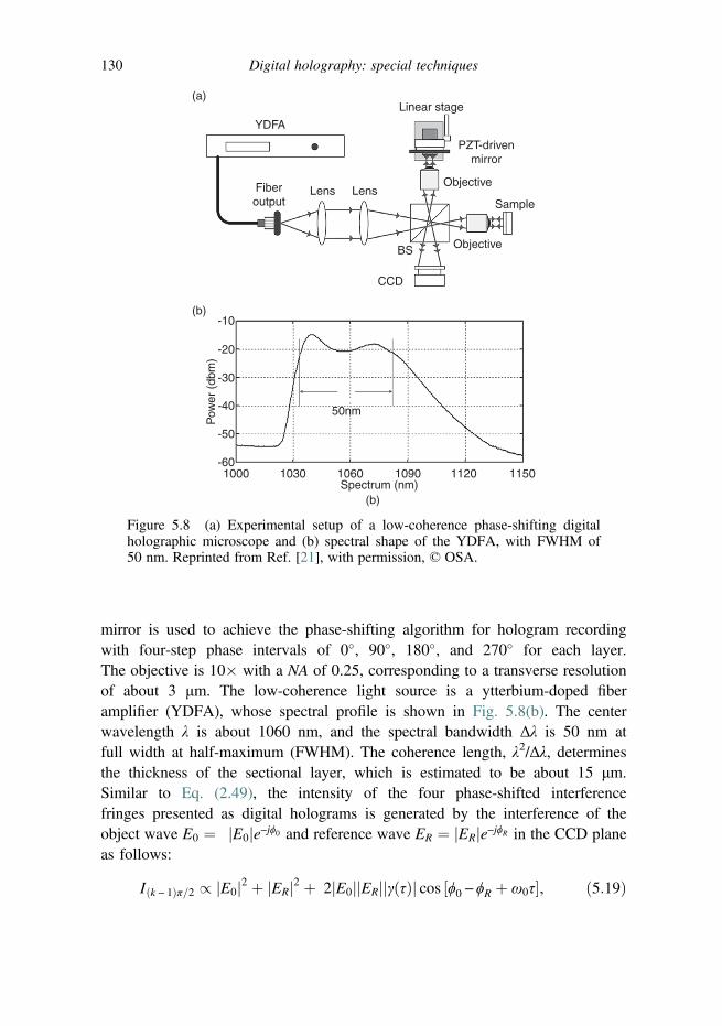
mirror is used to achieve the phase-shifting algorithm for hologram recordingwith four-step phase intervals of 0�, 90�, 180�, and 270� for each layer.The objective is 10� with a NA of 0.25, corresponding to a transverse resolutionof about 3 μm. The low-coherence light source is a ytterbium-doped fiberamplifier (YDFA), whose spectral profile is shown in Fig. 5.8(b). The centerwavelength λ is about 1060 nm, and the spectral bandwidth Δλ is 50 nm atfull width at half-maximum (FWHM). The coherence length, λ2/Δλ, determinesthe thickness of the sectional layer, which is estimated to be about 15 μm.Similar to Eq. (2.49), the intensity of the four phase-shifted interferencefringes presented as digital holograms is generated by the interference of theobject wave E0 ¼ jE0je−jϕ0 and reference wave ER ¼ jERje−jϕR in the CCD planeas follows:

Iðk − 1Þπ=2 / jE0j2 þ jERj2 þ 2jE0jjERjjγ τð Þj cos ½ϕ0 −ϕR þ ω0τ�, ð5:19Þ

YDFA

Linear stage

PZT-drivenmirror

Objective

ObjectiveBS

LensLensFiberoutput

CCD

-10

-20

-30

-40

-50

-601000 1030 1060 1090 1120 1150

Spectrum (nm)

50nm

Pow

er (

dbm

)

(a)

(b)

(b)

Sample

Figure 5.8 (a) Experimental setup of a low-coherence phase-shifting digitalholographic microscope and (b) spectral shape of the YDFA, with FWHM of50 nm. Reprinted from Ref. [21], with permission, © OSA.


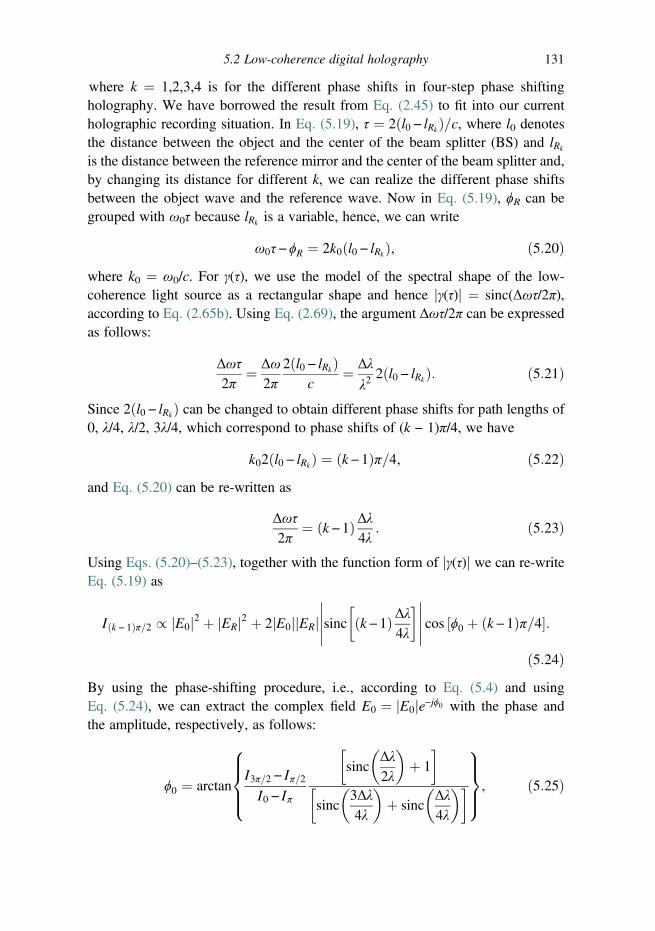
where k ¼ 1,2,3,4 is for the different phase shifts in four-step phase shiftingholography. We have borrowed the result from Eq. (2.45) to fit into our currentholographic recording situation. In Eq. (5.19), τ ¼ 2ðl0 − lRkÞ=c, where l0 denotesthe distance between the object and the center of the beam splitter (BS) and lRk

is the distance between the reference mirror and the center of the beam splitter and,by changing its distance for different k, we can realize the different phase shiftsbetween the object wave and the reference wave. Now in Eq. (5.19), ϕR can begrouped with ω0τ because lRk is a variable, hence, we can write

ω0τ −ϕR ¼ 2k0ðl0 − lRkÞ, ð5:20Þwhere k0 ¼ ω0/c. For γ(τ), we use the model of the spectral shape of the low-coherence light source as a rectangular shape and hence jγ(τ)j ¼ sinc(Δωτ/2π),according to Eq. (2.65b). Using Eq. (2.69), the argument Δωτ/2π can be expressedas follows:

Δωτ2π

¼ Δω2π

2ðl0 − lRkÞc

¼ Δλ

λ22ðl0 − lRkÞ: ð5:21Þ

Since 2ðl0 − lRkÞ can be changed to obtain different phase shifts for path lengths of0, λ/4, λ/2, 3λ/4, which correspond to phase shifts of (k − 1)π/4, we have

k02ðl0 − lRkÞ ¼ ðk −1Þπ=4, ð5:22Þand Eq. (5.20) can be re-written as

Δωτ2π

¼ k −1ð ÞΔλ4λ

: ð5:23Þ

Using Eqs. (5.20)–(5.23), together with the function form of jγ(τ)j we can re-writeEq. (5.19) as

Iðk − 1Þπ=2 / jE0j2 þ jERj2 þ 2jE0jjERj sinc k − 1ð ÞΔλ4λ

� �� cos ½ϕ0 þ k −1ð Þπ=4�:

ð5:24ÞBy using the phase-shifting procedure, i.e., according to Eq. (5.4) and usingEq. (5.24), we can extract the complex field E0 ¼ jE0je−jϕ0 with the phase andthe amplitude, respectively, as follows:

ϕ0 ¼ arctanI3π=2 − Iπ=2I0 − Iπ

sincΔλ2λ

� þ 1

� �

sinc3Δλ4λ

� þ sinc

Δλ4λ

� � �8>><>>:

9>>=>>;, ð5:25Þ


and

jE0j ¼

ffiffiffiffiffiffiffiffiffiffiffiffiffiffiffiffiffiffiffiffiffiffiffiffiffiffiffiffiffiffiffiffiffiffiffiffiffiffiffiffiffiffiffiffiffiffiffiffiffiffiffiffiffiffiffiffiffiffiffiffiffiffiffiffiffiffiffiffiffiffiffiffiffiffiffiffiffiffiffiffiffiffiffiffiffiffiffiffiffiffiffiffiffiffiffiffiffiffiffiffiffiffiffiffiffiffiffiffiffiffiffiffiffiffiffiffiffiffiffiffiffiffiffiffiffiffiffiffiffiffiffiffiffiffiffiffiffiffiffiffiffiffiI3π=2−Iπ=2� �

sincΔλ2λ

� þ1

� �� 2

þ I0−Iπð Þ sinc3Δλ4λ

� þ sinc

Δλ4λ

� � �� 2s

2 sincΔλ2λ

� þ1

� �sinc

3Δλ4λ

� þ sinc

Δλ4λ

� � �ð5:26Þ

by assuming ER ¼ 1.Figure 5.9 shows a tranquilized zebra fish. Holograms were captured using the

CCD at 2.5 frames/second. Figure 5.10(a) shows a portion of the tail of the zebrafish where holograms were captured, and Fig. 5.10(b) – (d) show three opticalsections. Clearly, in Fig. 5.10(d), we see the outline of the spine at that section.Figure 5.11 shows the phase plot at the section z ¼ 60 μm, where the spine isclearly outlined.

Current low-coherence holographic recording systems have a sectioning cap-ability of about 10–20 μm as is the case shown in the above results. When using anultra-wideband source, such as a supercontinuum of spectral bandwidth of about500 nm, a very short coherence length of the order of 1 μm is possible.

Figure 5.9 Image of a zebra fish. Reprinted from Ref. [21], with permission,© OSA.

Reconstruction (low coherence)

85µm 85µm 85µm

(a)

(b) (c) (d)z=0 µm z=30 µm z=60 µm

Figure 5.10 (a) Portion of the tail to be recorded holographically. (b)–(d)Optical sections at three different sections. Reprinted from Ref. [21], withpermission, © OSA.


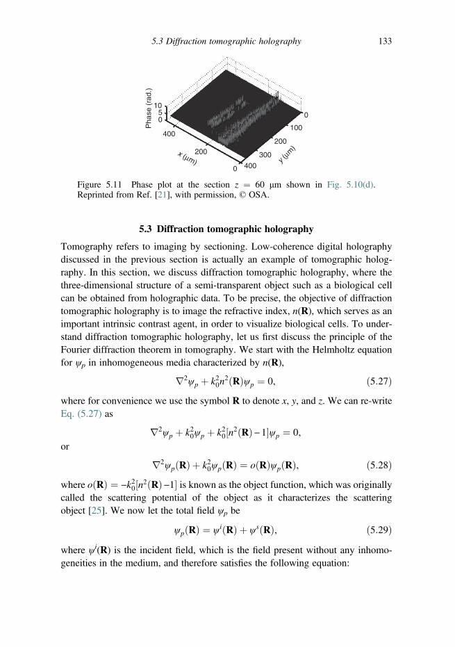
5.3 Diffraction tomographic holography

Tomography refers to imaging by sectioning. Low-coherence digital holographydiscussed in the previous section is actually an example of tomographic holog-raphy. In this section, we discuss diffraction tomographic holography, where thethree-dimensional structure of a semi-transparent object such as a biological cellcan be obtained from holographic data. To be precise, the objective of diffractiontomographic holography is to image the refractive index, n(R), which serves as animportant intrinsic contrast agent, in order to visualize biological cells. To under-stand diffraction tomographic holography, let us first discuss the principle of theFourier diffraction theorem in tomography. We start with the Helmholtz equationfor ψp in inhomogeneous media characterized by n(R),

r2ψp þ k20n2ðRÞψp ¼ 0, ð5:27Þ

where for convenience we use the symbol R to denote x, y, and z. We can re-writeEq. (5.27) as

r2ψp þ k20ψp þ k20½n2 Rð Þ−1�ψp ¼ 0,

or

r2ψp Rð Þ þ k20ψpðRÞ ¼ o Rð ÞψpðRÞ, ð5:28Þwhere o Rð Þ ¼ −k20½n2 Rð Þ−1� is known as the object function, which was originallycalled the scattering potential of the object as it characterizes the scatteringobject [25]. We now let the total field ψp be

ψp Rð Þ ¼ ψi Rð Þ þ ψs Rð Þ, ð5:29Þwhere ψi(R) is the incident field, which is the field present without any inhomo-geneities in the medium, and therefore satisfies the following equation:

Pha

se (

rad.

)

0

105

200

400

0y (

µm)

x (µm) 400

300

200

100

0

Figure 5.11 Phase plot at the section z ¼ 60 μm shown in Fig. 5.10(d).Reprinted from Ref. [21], with permission, © OSA.

5.3 Diffraction tomographic holography 133

r2ψi Rð Þ þ k20ψiðRÞ ¼ 0: ð5:30Þ

ψs(R) is the scattered field, which is attributed entirely to the inhomogeneities. Bysubstituting Eq. (5.29) into Eq. (5.28), together with Eq. (5.30), we can obtain thefollowing equation for the scattered field:

r2ψs Rð Þ þ k20ψsðRÞ ¼ o Rð ÞψpðRÞ: ð5:31Þ

A solution to the above scalar Helmholtz equation can be written in terms of theGreen function. The Green function, G(R, R0), is a solution of the followingequation:

r2G R,R0ð Þ þ k20GðR,R0Þ ¼ δðR−R0Þ ð5:32Þwith

G R,R0ð Þ ¼ −e−jk0jR −R0j

4πjR−R0j ¼ G jR−R0jð Þ:

Now, the source term in Eq. (5.31) can be written as a collection of impulsesweighted by o(R0) ψp(R0) and shifted by R0:

o Rð Þψp Rð Þ ¼ðo R0ð Þψp R0ð Þδ R−R0ð Þd3R0: ð5:33Þ

Therefore, the solution to Eq. (5.31) can be written as

ψs Rð Þ ¼ðG R−R0ð Þo R0ð Þψp R0ð Þd3R0: ð5:34Þ

Note that in Eq. (5.34), we still have the unknown total field, ψp(R0). To find thesolution to the scattered field, we make use of one of the simplest approximationscalled the first Born approximation. Other approximations such as the first Rytovapproximation have also been used to estimate the solution to the scattered field[26]. The first Born approximation states that the scattered field is much weakerthan the incident field, i.e.,

ψs Rð Þ � ψp Rð Þ: ð5:35ÞUnder this approximation, we can replace ψp(R) by ψi(R) in Eq. (5.34) to obtainthe Born approximation of the scattered field, given by

ψs Rð Þ ¼ðG R−R0ð Þo R0ð Þψi R0ð Þd3R0: ð5:36Þ

Based on the above result, we will now derive what is known as the Fourierdiffraction theorem in tomography. The theorem will relate the Fourier transformof the scattered field to the three-dimensional Fourier transform of the object


function. The Green function is a spherical wave and we now introduce Weyl’splane wave expansion of a spherical wave [27]:

G jR−R0jð Þ ¼ −e−jk0jR −R0j

4πjR−R0j ¼j

8π2

ðð∞−∞

e−j½kx x − x0ð Þþky y − y0ð Þþkz z − z0ð Þ�ffiffiffiffiffiffiffiffiffiffiffiffiffiffiffiffiffiffiffiffiffik20 − k

2x − k

2y

q dkx dky, ð5:37Þ

where kz ¼ffiffiffiffiffiffiffiffiffiffiffiffiffiffiffiffiffiffiffiffiffik20 − k

2x − k

2y

qunder the restriction that k2x þ k2y þ k2z < k20 so that

evanescent waves are ignored. Now assuming that the incident field is a planewave propagating along the z-direction, i.e., ψi Rð Þ ¼ e−jk0z, and measuring thescattered field at z ¼ l as shown in Fig. 5.12, Eq. (5.36) becomes

ψs x, y; z¼ lð Þ ¼ðð ð∞

−∞

j

8π2

ðð∞−∞

e−j kx x − x0ð Þþky y − y0ð Þþkz l − z0ð Þ½ �ffiffiffiffiffiffiffiffiffiffiffiffiffiffiffiffiffiffiffiffiffik20−k

2x −k

2y

q dkx dky o x0, y0, z0ð Þe−jk0z0264

375

dx0dy0dz0: ð5:38Þ

We evaluate the primed variables first, having the following three-dimensionalFourier transform of o x, y, zð Þe−jk0z:

Figure 5.12 The two-dimensional scattered field spectrum along the plane z ¼ lis related to the Fourier transform of the object on the surface of the Ewald sphere.

5.3 Diffraction tomographic holography 135

ððð∞−∞

ejkxx0þjkyy0þjkzz0o x0, y0, z0ð Þe−jk0z0 dx0dy0dz0 ¼ F 3D o x, y, z,ð Þe−jk0z� �

¼ O kx, ky, kz − k0� �

: ð5:39ÞPutting the above result into Eq. (5.38), we have

ψs x, y; z ¼ lð Þ ¼ j

8π2

ðð∞−∞

O kx, ky, kz − k0� �ffiffiffiffiffiffiffiffiffiffiffiffiffiffiffiffiffiffiffiffiffik20 − k

2x − k

2y

q e−jkxx − jkyy − jkzldkx dky

¼ j

2F −1 O kx, ky, kz − k0

� �ffiffiffiffiffiffiffiffiffiffiffiffiffiffiffiffiffiffiffiffiffik20 − k

2x − k

2y

q e − jffiffiffiffiffiffiffiffiffiffiffiffiffiffiffiffik20 − k2x − k2y

pl

8><>:

9>=>;,

which can be recognized as a two-dimensional Fourier transform as shown in thelast step of the equation. By taking the two-dimensional Fourier transform of theabove equation, we have

−2jF ψs x, y; z ¼ lð Þf gejffiffiffiffiffiffiffiffiffiffiffiffiffiffiffiffiffik20 − k2x − k2y

pl

ffiffiffiffiffiffiffiffiffiffiffiffiffiffiffiffiffiffiffiffiffik20 − k

2x − k

2y

q¼ O kx, ky, kz − k0

� �, ð5:40Þ

where we have used kz ¼ffiffiffiffiffiffiffiffiffiffiffiffiffiffiffiffiffiffiffiffiffik20 − k

2x − k

2y

q: Equation (5.40) is the Fourier diffraction

theorem as it relates the three-dimensional Fourier transform of the object functionto the two-dimensional Fourier transform of the field measured at the recordingdevice. Note that

kz ¼ffiffiffiffiffiffiffiffiffiffiffiffiffiffiffiffiffiffiffiffiffik20 − k

2x − k

2y

qð5:41Þ

is the Ewald equation, which says that the frequency spectrum is limited to a sphere,k2x þ k2y þ k2z ¼ k20 in the frequency domain, the so-called Ewald sphere. Hence,Eq. (5.40) states that the two-dimensional scattered field spectrum along the planez ¼ l is related to the Fourier transform of the object on the surface of the Ewaldsphere. The situation is shown in Fig. 5.12. For brevity, we only illustrate along twodirections x and z and therefore kx and kz, accordingly. The solid line of the Ewaldsphere can be considered transmission tomography, whereas the dotted line indi-cates reflection tomography where the measured field is on the plane z ¼ −l.

The power of diffraction tomography is that on rotating the object by 360degrees, each rotation will map different regions of the three-dimensional fre-quency spectrum of the object function. After a complete mapping by rotating, wecan take the inverse three-dimensional Fourier transform of the object function toget the three-dimensional complex refractive index. Figure 5.13 summarizes the


process of diffraction tomography, where the three-dimensional spectrum is filledwith eight rotations as an example with the object being rotated on the x–z plane.

In diffraction holographic tomography, we just need to record the complexscattered field ψs(x, y; z ¼ l) holographically for many incident angles and thenperform the Fourier diffraction theorem for reconstruction of the three-dimensionalobject.

5.4 Optical scanning holography

Optical scanning holography (OSH) is a unique digital holographic recordingtechnique proposed by Poon and Korpel [28, 29]. In OSH, a structured opticalbeam is produced by interference and the object target to be measured is rasterscanned using the interference pattern. Meanwhile, the hologram data are acquiredpixel by pixel. The hologram data can be directly displayed on a real-time

Figure 5.13 Summary of Fourier diffraction tomography.

5.4 Optical scanning holography 137

electronic device, such as a cathode-ray tube (CRT) monitor. Alternatively, thehologram data can be digitized and stored as a digital hologram in a computer.

OSH has several unique merits in comparison with conventional digitalholographic recording techniques. First, OSH does not rely on the interferencebetween the light scattered from an object and a reference light. So OSH can beapplied to remote sensing applications. In addition, OSH can be operated ineither the coherent mode or the incoherent mode. In the incoherent mode, thephase information of the object target is lost but the three-dimensional infor-mation is still recorded. So the incoherent-mode OSH can be used to acquirefluorescence holograms [30–33] in the field of bio-sensing. Moreover, theacquired hologram as well as the interference pattern applied in OSH canbe modified by adjusting the functional forms of the pupils in the OSH setup –

this is known as pupil-engineering or PSF-engineering [34, 35]. Using pupil-engineering, coding [34], cryptography [35], recognition [36], and filtering [37]can be performed on the fly during hologram acquisition. Moreover, superresolution [38, 39] and sectional reconstruction [40, 41] can be realized byemploying OSH. OSH also finds numerous applications in three-dimensionaldisplay and storage.

In this section we will only introduce the fundamental concept of OSH. Theadvanced properties and applications of OSH can be found in the above mentionedreferences or in Refs. [42–45].

5.4.1 Fundamental principles

Figure 5.14 depicts the typical setup of an optical scanning holographic system.The laser beam operated at angular frequency ω0 is separated into two beams by abeamsplitter (BS1). The transmitted light from BS1 (beam 1) is first collimated andthen passes through pupil p1 at the front focal plane of lens L1. The frequency ofthe reflected light from BS1 (beam 2) is shifted to ω0 þ Ω by an acousto-opticfrequency shifter (AOFS). The light is also collimated and passes through pupil p2at the front focal plane of lens L1. Beam 1 and beam 2 are combined bybeamsplitter BS2 in front of lens L1. Consequently, the complex field on theobject plane is given by

S x, y, zð Þ ¼ P1zk0x

f,k0y

f

� exp jω0tð Þ þ P2z

k0x

f,k0y

f

� exp j ω0 þ Ωð Þt½ �, ð5:42Þ

where Piz(k0x/f, k0y/f) is the optical field of beam 1 or 2 at a distance z awayfrom the back focal plane of L1, and through Fresnel diffraction [Eq. (1.35)], it isgiven by


Pizk0x

f,k0y

f

� ¼ Pi

k0x

f,k0y

f

� � h x, y; zð Þ, i ¼ 1, 2: ð5:43Þ

In the above equation Pi(k0x/f, k0y/f) is the optical field at the back focal plane oflens L1. According to the setup described in Fig. 5.14, and knowing that theFourier transform of the pupil in the front focal plane of a lens is the fielddistribution at the back focal plane of the lens [see Eq. (1.45)], we have

Pik0x

f,k0y

f

� ¼ F piðx,yÞf gj

kx¼k0xf ,ky¼

k0yf, i ¼ 1, 2 ð5:44Þ

where pi(x, y) is the pupil function at the front focal plane of L1.To find the complex field at the object plane, we consider a typical case, namely

the first pupil is considered clear, i.e., p1(x, y) ¼ 1, and the second pupil is apinhole, p2(x, y) ¼ δ(x, y). Therefore, beam 1 becomes a spherical wave behindlens L1, while beam 2 becomes a plane wave, as shown in Fig. 5.14. The opticalfield at z away from the focal plane of lens L1 is thus given by

S x, y; zð Þ ¼ jk02πz

exp−jk02z

x2 þ y2� ��

exp jω0tð Þ þ a exp j ω0 þ Ωð Þt½ �, ð5:45Þ

where a is a proportionality constant. The above equation is similar to Eq. (2.3) fora point-source hologram. The intensity on the object plane is

Figure 5.14 Schematic of optical scanning holography. BS beamsplitter;M mirror; BE beam expander; L lens; PD photodetector; BPF band-pass filter.


jS x,y; zð Þj2 ¼ jk02πz

exp

�−jk02z

x2 þ y2� ��

exp jω0tð Þ þ a exp j ω0 þ Ωð Þt½ ��

��2

¼ DC þ B sin

�k02z

x2 þ y2� �þ Ωt

�, ð5:46Þ

where B is also a proportionality constant. The pattern described in Eq. (5.46) is astatic Fresnel zone plate given by Eq. (2.4) when there is no temporal frequencyoffset between the two interfering beams, i.e., Ω ¼ 0, but when Ω 6¼ 0 we haverunning fringes that will be moving toward the center of the zone pattern and wecall this dynamic pattern the time-dependent Fresnel zone plate (TDFZP).

Upon producing the TDFZP, we use it to scan an object target with an amplitudetransparency of T(x, y; z). Scanning can be realized by moving the object target ona two-dimensional motorized stage, as shown in Fig. 5.14. Alternatively, we canalso move the TDFZP using x–y mirror galvanometer scanners. In both cases, arelative movement is produced between the object target and the TDFZP. At anymoment of the movement, there is a shift between the object target and the TDFZP.Assuming that the center of the object is moved from (x, y)¼ (0, 0) to (x, y)¼ (x0, y0),the light transmitted through (if the object target is transparent or semi-transparent)or scattered away from (if the object target is diffusely reflecting) the object targetwill be proportional to S(x, y; z)T(x − x0, y − y0; z). The lens L2 is used to collectthe transmitted or scattered light, while photodetector PD1 detects the light. Thephotodetector detects the intensity and integrates the intensity over its active surface,giving the output current i as

i x0, y0ð Þ / ΔjS x,y; zð ÞT xþ x0,yþ y0; zð Þj2dx dy dz: ð5:47ÞIn the above equation, we have modeled the three-dimensional object target as acollection of infinitely thin sections z away from the back focal plane of lens L1.Hence the integration over z, i.e., along the depth of the object, corresponds to therecording of a three-dimensional object. By substituting Eq. (5.45) into Eq. (5.47),we can separate Eq. (5.47) into two terms, the baseband current (DC current) iDCand the heterodyne current iΩ:

iDC x0, y0ð Þ /ðjP1zj2 � jTj2dzþ

ðjP2zj2 � jTj2dz, ð5:48aÞ

iΩ x0, y0ð Þ /ðP1zP

�2ze

−jΩt � jT j2dzþðP2zP

�1ze

jΩt � jT j2dz, ð5:48bÞ

where � denotes correlation involving the x0 and y0 coordinates. We can use abandpass filter (BPF) to filter out the DC current iDC. The remaining heterodynecurrent iΩ oscillating at frequency Ω is sent to a standard lock-in amplifier.


A diagram of the core circuit of the lock-in amplifier is shown in Fig. 5.15. Thiscircuit performs the so-called synchronous demodulation. Basically, a referencesignal, sin(Ωt), also oscillating at frequency Ω, is applied to the lock-in amplifier todemodulate the signal of interest. In practice, the reference signal comes fromanother fixed photodetector PD2, as shown in Fig. 5.14. In this way, any unwantedphase fluctuation within the interferometer (formed by beamsplitters BS1, BS2,and mirrors M1 and M2) can be compensated significantly.

For a general dual-channel lock-in amplifier, there are two outputs given by

Out1 / LPF iΩ � sin ðΩtÞf g, ð5:49aÞand

Out2 / LPF iΩ � cos ðΩtÞf g, ð5:49bÞwhere LPF{•} stands for the operator of lowpass filtering, i.e., any frequency ofΩ or higher will be filtered out and will not be present at the output of the filter.For convenience, we let P ¼ P1zP�

2z ¼ jPjexpðjΦÞ. Thus Eq. (5.48b) can be re-written as

iΩ ¼ ReðP� jT j2e−jΩtdz

n o¼

ðjPj cos ðΦ−ΩtÞ � jT j2dz: ð5:50Þ

By substituting Eq. (5.50) into Eqs. (5.49a) and (5.49b) and evoking the operationof lowpass filtering, we have

Out1 ¼ðjPj sinΦ� jT j2dz, ð5:51aÞ

Out2 ¼ðjPj cosΦ� jTj2dz, ð5:51bÞ

for the outputs of the lock-in amplifier. The two outputs can be converted to digitalsignals by an analog-to-digital converter (ADC), and therefore can be transmittedor processed digitally.

Figure 5.15 Circuit diagram of a lock-in amplifier.


5.4.2 Hologram construction and reconstruction

To construct a hologram of the scanned object target, we can combine the twooutputs from Eqs. (5.51a) and (5.51b) digitally to generate a digital complexhologram Hc as

Hc ¼ Out2 þ j� Out1 ¼ðP� jT j2dz: ð5:52Þ

To see the effect of retrieving the three-dimensional location of the object target,we assume that the object is located at z ¼ z0 and its amplitude transmittance canbe expressed as T(x, y; z) ¼ T(x, y) � δ(z − z0). Hence Eq. (5.52) can be reduced to

Hcðx, yÞ ¼ Pðx, y; z0Þ � jTðx,yÞj2, ð5:53Þwhere P x, y; z0ð Þ ¼ P1z0P

�2z0 : In the typical case described in Fig. 5.14, beam 1 is a

spherical wave on the object target, i.e., p1(x, y) ¼ 1, and beam 2 is a plane wave,i.e., p2(x, y) ¼ δ(x, y), and according to Eq. (5.43) we have

P x, y; z0ð Þ ¼ P1z0 ¼ h x, y; z0ð Þ: ð5:54ÞAs a result, Eq. (5.53) can be expressed as

Hcðx, yÞ ¼ h x, y; z0ð Þ � jTðx,yÞj2: ð5:55ÞWe can easily identify Hc(x, y) as the complex hologram of jT(x, y)j2. Thus we canapply the Fresnel diffraction formula [Eq. (1.35)] to retrieve the field distribution atany plane of interest away from the hologram, i.e.,

ψp x, y; zrð Þ / h x, y; zrð Þ � h x, y; z0ð Þ � jT x,yð Þj2h i

, ð5:56Þ

where zr is the distance measured from the hologram plane. Apparently, theintensity distribution of the object target can be reconstructed at zr ¼ z0 becauseψp(x, y; z0)¼ jT(x, y)j2. This is a real image of the reconstruction [see Problem 5.5].If we reconstruct H�

cðx, yÞ, the reconstruction is a virtual image.It is noted that the reconstruction process of optical scanning holography (OSH)

is exactly the same as that in conventional holography. But in OSH there is noannoying zeroth-order beam and twin image among the reconstructed field. This isthe main merit of the complex hologram. Also we note that in the above processonly the intensity distribution of the object target jT(x, y)j2 is retrieved. Indeed,because the phase of the object T(x, y) is not recorded, OSH is operated in theincoherent mode. However, the phase of the object target can also be recorded,provided a pinhole mask is attached to photodetector PD1 located at the back focalplane of lens L2 [46]. We will not discuss the details here but only show theresults. The resulting two outputs become


Out1 ¼ðjPj sinΦ� T dz, ð5:57aÞ

Out2 ¼ðjPj cosΦ� T dz: ð5:57bÞ

Similar to the incoherent mode, we can combine the two outputs to produce Hc,

Hc ¼ Out2 þ j� Out1 ¼ðP� T dz: ð5:58Þ

It is noted that now Hc is the complex hologram of T and OSH is operated in thecoherent mode. Figure 5.16 shows the reconstruction of a complex hologram givenby Eq. (5.58), which is recorded in the coherent mode [47], while in Fig. 5.17 weshow the holograms and reconstruction of a diffusely reflecting object (a die),illustrating the incoherent operation of optical scanning holography as the recon-struction is free of the speckle noise commonly exhibited in coherent opticalsystems [48]. Figure 5.7(a) and (b) are the real and imaginary parts of the complexhologram given by Eq. (5.52), respectively, where the real part of the hologram isgiven by Eq. (5.51b) and the imaginary part is given by Eq. (5.51a). Digitalreconstruction of the complex hologram is shown in Fig. 5.7(c), which is obviouslynot contaminated by speckle noise as compared to the image shown in Fig. 5.17(d)where the image is observed by a CCD camera upon coherent illumination of thedie. Reference [49] is the most recent review paper on optical scanningholography.

0

20

40

60

80

100

1200 20 40 60

(a) (b)

80 100 120

10

0

-10150

150

100

100

5050

0 0

phas

e (r

ad)

x (µm) y (µm) x (µm)

y (µ

m)

Figure 5.16 Reconstruction of a hologram recorded in coherent mode. Thespecimen is a good phase object: siliceous three-pronged spongilla spicule. (a)Absolute value of the reconstruction amplitude, and (b) three-dimensional phaseprofile of the specimen. Reprinted from Ref. [47], with permission.


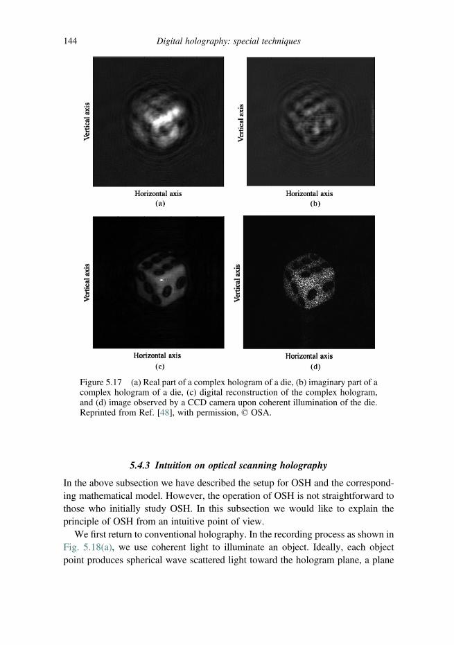
5.4.3 Intuition on optical scanning holography

In the above subsection we have described the setup for OSH and the correspond-ing mathematical model. However, the operation of OSH is not straightforward tothose who initially study OSH. In this subsection we would like to explain theprinciple of OSH from an intuitive point of view.

We first return to conventional holography. In the recording process as shown inFig. 5.18(a), we use coherent light to illuminate an object. Ideally, each objectpoint produces spherical wave scattered light toward the hologram plane, a plane

Figure 5.17 (a) Real part of a complex hologram of a die, (b) imaginary part of acomplex hologram of a die, (c) digital reconstruction of the complex hologram,and (d) image observed by a CCD camera upon coherent illumination of the die.Reprinted from Ref. [48], with permission, © OSA.


Figure 5.18 Recording for (a) a conventional hologram, (b) a scanning holo-gram at x10, and (c) a scanning hologram at x20.


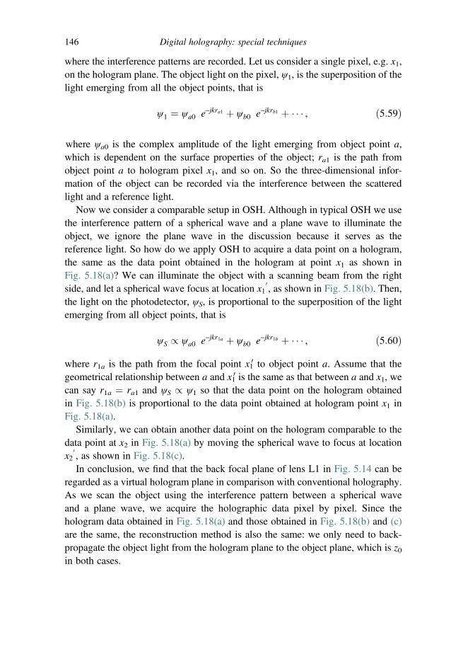
where the interference patterns are recorded. Let us consider a single pixel, e.g. x1,on the hologram plane. The object light on the pixel, ψ1, is the superposition of thelight emerging from all the object points, that is

ψ1 ¼ ψa0 e−jkra1 þ ψb0 e−jkrb1 þ , ð5:59Þ

where ψa0 is the complex amplitude of the light emerging from object point a,which is dependent on the surface properties of the object; ra1 is the path fromobject point a to hologram pixel x1, and so on. So the three-dimensional infor-mation of the object can be recorded via the interference between the scatteredlight and a reference light.

Now we consider a comparable setup in OSH. Although in typical OSH we usethe interference pattern of a spherical wave and a plane wave to illuminate theobject, we ignore the plane wave in the discussion because it serves as thereference light. So how do we apply OSH to acquire a data point on a hologram,the same as the data point obtained in the hologram at point x1 as shown inFig. 5.18(a)? We can illuminate the object with a scanning beam from the rightside, and let a spherical wave focus at location x1

0, as shown in Fig. 5.18(b). Then,

the light on the photodetector, ψS, is proportional to the superposition of the lightemerging from all object points, that is

ψS / ψa0 e−jkr1a þ ψb0 e−jkr1b þ , ð5:60Þ

where r1a is the path from the focal point x10 to object point a. Assume that thegeometrical relationship between a and x10 is the same as that between a and x1, wecan say r1a ¼ ra1 and ψS / ψ1 so that the data point on the hologram obtainedin Fig. 5.18(b) is proportional to the data point obtained at hologram point x1 inFig. 5.18(a).

Similarly, we can obtain another data point on the hologram comparable to thedata point at x2 in Fig. 5.18(a) by moving the spherical wave to focus at locationx2

0, as shown in Fig. 5.18(c).In conclusion, we find that the back focal plane of lens L1 in Fig. 5.14 can be

regarded as a virtual hologram plane in comparison with conventional holography.As we scan the object using the interference pattern between a spherical waveand a plane wave, we acquire the holographic data pixel by pixel. Since thehologram data obtained in Fig. 5.18(a) and those obtained in Fig. 5.18(b) and (c)are the same, the reconstruction method is also the same: we only need to back-propagate the object light from the hologram plane to the object plane, which is z0in both cases.


Problems

5.1 Show that, in three-step phase-shifting holography, the complex amplitude ofthe object is given by

ψo ¼ð1þ jÞ I0−Iπ=2

� �þ ð j−1ÞðIπ−Iπ=2Þ4ψ�

r

,

where the three holograms are

Iδ ¼ jψo þ ψr exp −jδð Þj2

with phase steps δ ¼ 0, δ ¼ π/2, and δ ¼ π. ψr is the complex amplitude of thereference light.

5.2 If the phase steps in three-step phase-shifting holography are 0, δ1, and δ2, findthe complex amplitude of the object, ψo, in terms of two intensity maps, i.e.,jψoj2 and jψrj2, three holograms, and two phase steps δ1 and δ2. ψr is thecomplex amplitude of the reference light.

5.3 Prove that for two-step phase-shifting holography [Eq. (5.16)], π/2 is the phasestep that is most insensitive to the phase error.

5.4 The heterodyne current from optical scanning holography is given byEq. (5.50) as follows:

iΩ ¼ ReðP� jT j2e−jΩtdz

n o:

Show that the two outputs from a dual channel lock-in amplifier are given by

Out1 ¼ðjPj sinΦ� jT j2dz,

Out2 ¼ðjPj cosΦ� jTj2dz:

5.5 (a) Prove that

f 1 xð Þ � f 2 xð Þ ¼ f �1 −xð Þ � f 2 xð Þ,

where � and * are the operators of correlation and convolution, respectively,and defined according to Table 1.1.(b) Apply the result in part (a), and prove that

h x, y; z0ð Þ � h x, y; z0ð Þ � jT x,yð Þj2h i

¼ jT x,yð Þj2:

Problems 147

References

1. I. Yamaguchi, and T. Zhang, Phase-shifting digital holography, Optics Letters 22,1268–1270 (1997).

2. T. Zhang, and I. Yamaguchi, Three-dimensional microscopy with phase-shiftingdigital holography, Optics Letters 23, 1221–1223 (1998).

3. I. Yamaguchi, J.-I. Kato, S. Ohta, and J. Mizuno, Image formation in phase-shiftingdigital holography and applications to microscopy, Applied Optics 40, 6177–6186(2001).

4. J. Rosen, G. Indebetouw, and G. Brooker, Homodyne scanning holography, OpticsExpress 14, 4280–4285 (2006).

5. M. Gross, and M. Atlan, Digital holography with ultimate sensitivity, Optics Letters32, 909–911 (2007).

6. P. Guo, and A. J. Devaney, Digital microscopy using phase-shifting digital holog-raphy with two reference waves, Optics Letters 29, 857–859 (2004).

7. J.-P. Liu, T.-C. Poon, G.-S. Jhou, and P.-J. Chen, Comparison of two-, three-, andfour-exposure quadrature phase-shifting holography, Applied Optics 50, 2443–2450(2011).

8. M. Atlan, M. Gross, and E. Absil, Accurate phase-shifting digital interferometry,Optics Letters 32, 1456–1458 (2007).

9. V. Micó, J. García, Z. Zalevsky, and B. Javidi, Phase-shifting Gabor holography,Optics Letters 34, 1492–1494 (2009).

10. J.-P. Liu, and T.-C. Poon, Two-step-only quadrature phase-shifting digital holography,Optics Letters 34, 250–252 (2009).

11. X. F. Meng, L. Z. Cai, X. F. Xu, X. L. Yang, X. X. Shen, G. Y. Dong, and Y. R.Wang, Two-step phase-shifting interferometry and its application in image encryption,Optics Letters 31, 1414–1416 (2006).

12. X. F. Meng, X. Peng, L. Z. Cai, A. M. Li, J. P. Guo, and Y. R. Wang, Wavefrontreconstruction and three-dimensional shape measurement by two-step dc-term-suppressed phase-shifted intensities, Optics Letters 34, 1210–1212 (2009).

13. C.-S. Guo, L. Zhang, H.-T. Wang, J. Liao, and Y. Y. Zhu, Phase-shifting error andits elimination in phase-shifting digital holography, Optics Letters 27, 1687–1689(2002).

14. W. Chen, C. Quan, C. J. Tay, and Y. Fu, Quantitative detection and compensation ofphase-shifting error in two-step phase-shifting digital holography, Optics Communi-cations 282, 2800–2805 (2009).

15. Y. Awatsuji, T. Tahara, A. Kaneko, T. Koyama, K. Nishio, S. Ura, T. Kubota, and O.Matoba, Parallel two-step phase-shifting digital holography, Applied Optics 47,D183–D189 (2008).

16. Y. Awatsuji, A. Fujii, T. Kubota, and O. Matoba, Parallel three-step phase-shiftingdigital holography, Applied Optics 45, 2995–3002 (2006).

17. T. Tahara, K. Ito, T. Kakue, M. Fujii, Y. Shimozato, Y. Awatsuji, K. Nishio, S. Ura, T.Kubota, and O. Matoba, Parallel phase-shifting digital holographic microscopy,Biomedical Optics Express 1, 610–616 (2010).

18. T. Kakue, Y. Moritani, K. Ito, Y. Shimozato, Y. Awatsuji, K. Nishio, S. Ura, T.Kubota, and O. Matoba, Image quality improvement of parallel four-step phase-shifting digital holography by using the algorithm of parallel two-step phase-shiftingdigital holography, Optics Express 18, 9555–9560 (2010).

19. T. Tahara, K. Ito, M. Fujii, T. Kakue, Y. Shimozato, Y. Awatsuji, K. Nishio, S. Ura, T.Kubota, and O. Matoba, Experimental demonstration of parallel two-step phase-shifting digital holography, Optics Express 18, 18975–18980 (2010).


20. T. Nomura, and M. Imbe, Single-exposure phase-shifting digital holography using arandom-phase reference wave, Optics Letters 35, 2281–2283 (2010).

21. Y.-C. Lin, C.-J. Cheng, and T.-C. Poon, Optical sectioning with a low-coherence phase-shifting digital holographic microscope, Applied Optics 50, B25–B30 (2011).

22. P. Massatsch, F. Charrière, E. Cuche, P. Marquet, and C. D. Depeursinge, Time-domain optical coherence tomography with digital holographic microscopy, AppliedOptics 44, 1806–1812 (2005).

23. S. Tamano, Y. Hayasaki, and N. Nishida, Phase-shifting digital holography witha low-coherence light source for reconstruction of a digital relief object hiddenbehind a light-scattering medium, Applied Optics 45, 953–959 (2006).

24. G. Pedrini, and H. J. Tiziani, Short-coherence digital microscopy by use of a lenslessholographic imaging system, Applied Optics 41, 4489–4496 (2002).

25. E. Wolf, Three-dimensional structure determination of semi-transparent objects fromholographic data, Optics Communications 1, 153–156 (1969).

26. Y. Sung, W. Choi, C. Fang-Yen, K. Badizadegan, R. R. Dasari, and M. S. Feld,Optical diffraction tomography for high resolution live cell imaging, Optics Express17, 266–277 (2009).

27. J. J. Stamnes, Focusing of a perfect wave and the airy pattern formula, OpticsCommunications 37, 311–314 (1981).

28. T.-C. Poon, and A. Korpel, Optical transfer function of an acousto-optic heterodyningimage processor, Optics Letters 4, 317–319 (1979).

29. T.-C. Poon, Scanning holography and two-dimensional image processing by acousto-optic two-pupil synthesis, Journal of the Optical Society of America A 2, 521–527(1985).

30. G. Indebetouw, T. Kim, T.-C. Poon, and B. W. Schilling, Three-dimensional locationof fluorescent inhomogeneities in turbid media by scanning heterodyne holography,Optics Letters 23, 135–137 (1998).

31. B. W. Schilling, T.-C. Poon, G. Indebetouw, B. Storrie, K. Shinoda, Y. Suzuki, andM. H. Wu, Three-dimensional holographic fluorescence microscopy, Optics Letters22, 1506–1508 (1997).

32. G. Indebetouw, and W. Zhong, Scanning holographic microscopy of three-dimensional fluorescent specimens, Journal of the Optical Society of America A 23,1699–1707 (2006).

33. G. Indebetouw, A posteriori quasi-sectioning of the three-dimensional reconstructionsof scanning holographic microscopy, Journal of the Optical Society of America A 23,2657–2661 (2006).

34. Y. Shinoda, J.-P. Liu, P. Sheun Chung, K. Dobson, X. Zhou, and T.-C. Poon, Three-dimensional complex image coding using a circular Dammann grating, Applied Optics50, B38–B45 (2011).

35. T.-C. Poon, T. Kim, and K. Doh, Optical scanning cryptography for secure wirelesstransmission, Applied Optics 42, 6496–6503 (2003).

36. T.-C. Poon, and T. Kim, Optical image recognition of three-dimensional objects,Applied Optics 38, 370–381 (1999).

37. J.-P. Liu, C.-C. Lee, Y.-H. Lo, and D.-Z. Luo, Vertical-bandwidth-limited digitalholography, Optics Letters 37, 2574–2576 (2012).

38. G. Indebetouw, A. El Maghnouji, and R. Foster, Scanning holographic microscopywith transverse resolution exceeding the Rayleigh limit and extended depth of focus,Journal of the Optical Society of America A 22, 892–898 (2005).

Problems 149

39. G. Indebetouw, Y. Tada, J. Rosen, and G. Brooker, Scanning holographic microscopywith resolution exceeding the Rayleigh limit of the objective by superposition ofoff-axis holograms, Applied Optics 46, 993–1000 (2007).

40. H. Kim, S.-W. Min, B. Lee, and T.-C. Poon, Optical sectioning for optical scanningholography using phase-space filtering with Wigner distribution functions, AppliedOptics 47, D164–D175 (2008).

41. E. Y. Lam, X. Zhang, H. Vo, T.-C. Poon, and G. Indebetouw, Three-dimensionalmicroscopy and sectional image reconstruction using optical scanning holography,Applied Optics 48, H113–H119 (2009).

42. T.-C. Poon, Optical Scanning Holography with MATLAB (Springer, New York, 2007).43. G. Indebetouw, The multi-functional aspect of scanning holographic microscopy:

a review, Chinese Optics Letters 7, 1066–1071 (2009).44. T.-C. Poon, Recent progress in optical scanning holography, Journal of Holography

and Speckle 1, 6–25 (2004).45. T.-C. Poon, Optical scanning holography: principles and applications, in Three-

Dimensional Holographic Imaging, C. J. Kuo, and M. H. Tsai, eds. (John Wiley &Sons, New York, 2002), pp. 49–75.

46. T.-C. Poon, and G. Indebetouw, Three-dimensional point spread functions of anoptical heterodyne scanning image processor, Applied Optics 42, 1485–1492 (2003).

47. G. Indebetouw, Y. Tada, and J. Leacock, Quantitative phase imaging with scanningholographic microscopy: an experimental assessment, BioMedical EngineeringOnLine 5, 63 (2006).

48. Y. S. Kim, T. Kim, S. S. Woo, H. Kang, T.-C. Poon, and C. Zhou, Speckle-free digitalholographic recording of a diffusely reflecting object, Optics Express 21, 8183–8189(2013).

49. T.-C. Poon, Optical scanning holography – a review of recent progress, Journal of theOptical Society of Korea 13, 406–415 (2009).


6

Applications in digital holography

In this chapter, we discuss some of the important and modern applications indigital holography, including holographic microscopy, sectioning, phase extrac-tion, optical contouring, and deformation measurements.

6.1 Holographic microscopy

The first Gabor hologram was invented as a new microscopic technique [1], but itsuffers from the problem of twin image. In 1965, a successful holographic micro-scope was demonstrated by E. Leith and J. Upatnieks [2]. However, the use ofholographic microscopy is limited by its inconvenient chemical developing pro-cedures. This drawback is apparently disappearing in the era of digital holography.Digital holographic microscopy (DHM) has unique merits in comparison withtraditional optical microscopy. DHM can acquire the three-dimensional informa-tion of a sample simultaneously, and the phase of the sample can be determinedquantitatively. DHM has become one of the most important applications in digitalholography. In DHM, some effort must be made to achieve micrometer or submicro-meter resolution. According to the recording geometry, DHM can be categorizedinto three types [OSH, see Section 5.4, is not taken into account here]: microscope-based DHM [3–8], Fourier-based DHM [9–14], and spherical-reference-basedDHM [15]. In the following sections, we discuss the three kinds of DHM.

6.1.1 Microscope-based digital holographic microscopy

Figure 6.1 depicts the setup of a typical transmission-type microscope-baseddigital holographic microscope. The mirror (M) in the reference arm can be tiltedfor off-axis holographic recording, or can be movable for phase-shifting record-ings. In the specimen arm, a microscope objective (MO) is used to produce amagnified image of the specimen. The digital holographic recording geometry can

151

also be realized as a reflection-type setup, as shown in Fig. 6.2. In the reflection-type setup, the object light is back-scattered to provide the object field to the CCD.Because the MO is in the path of the back-scattered object field, lens L is usedadditionally to provide uniform illumination of the specimen.

For both cases, the geometrical relation between the specimen and its image isshown in Fig. 6.3(a). Note that we do not need to focus the image on the CCDplane because the image is holographically recorded. Under the paraxial approxi-mation, the lateral magnification of the image is defined as

MLat ¼ −dido

¼ −θoθi, ð6:1Þ

Figure 6.1 Setup of a transmission-type microscope-based digital holographicmicroscope. BE beam expander; BS beamsplitter; M mirror; MO microscopeobjective.

Figure 6.2 Setup of a reflection-type microscope-based digital holographicmicroscope. BE beam expander; BS beamsplitter; M mirror; L lens; MO micro-scope objective.

152 Applications in digital holography

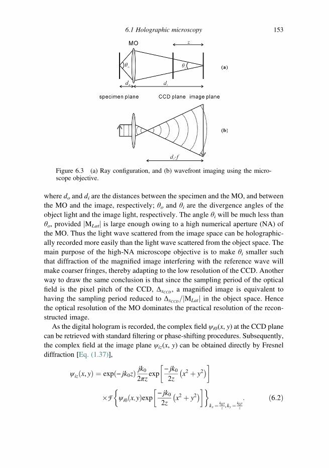
where do and di are the distances between the specimen and the MO, and betweenthe MO and the image, respectively; θo and θi are the divergence angles of theobject light and the image light, respectively. The angle θi will be much less thanθo, provided jMLatj is large enough owing to a high numerical aperture (NA) ofthe MO. Thus the light wave scattered from the image space can be holographic-ally recorded more easily than the light wave scattered from the object space. Themain purpose of the high-NA microscope objective is to make θi smaller suchthat diffraction of the magnified image interfering with the reference wave willmake coarser fringes, thereby adapting to the low resolution of the CCD. Anotherway to draw the same conclusion is that since the sampling period of the opticalfield is the pixel pitch of the CCD, ΔxCCD , a magnified image is equivalent tohaving the sampling period reduced to ΔxCCD=jMLatj in the object space. Hencethe optical resolution of the MO dominates the practical resolution of the recon-structed image.

As the digital hologram is recorded, the complex field ψi0(x, y) at the CCD planecan be retrieved with standard filtering or phase-shifting procedures. Subsequently,the complex field at the image plane ψiz(x, y) can be obtained directly by Fresneldiffraction [Eq. (1.37)],

ψizðx, yÞ ¼ exp − jk0zð Þ jk02πz

exp

�− jk02z

x2 þ y2� ��

�F ψi0 x,yð Þexp�− jk02z

x2 þ y2� ��

kx ¼ k0xz ,ky ¼

k0yz

: ð6:2Þ

Figure 6.3 (a) Ray configuration, and (b) wavefront imaging using the micro-scope objective.

6.1 Holographic microscopy 153

However, since conventional digital holographic recordings like that beingdiscussed are coherent imaging, the phase distribution of the magnified imageneeds to be considered carefully. According to geometrical optics and referring toFig. 6.3(a), we can find the image plane according to

1do

þ 1di

¼ 1f, ð6:3Þ

where f is the focal length of the MO. On the other hand, wavefront imaging by theMO is shown in Fig. 6.3(b), where we assume a flat object wavefront beingcoherently imaged. We note that on the image plane, there is a quadratic phaseerror. This phase error can be calculated rigorously using Fourier optics [16].Intuitively, we can say that the phase error is due to a divergent sphericalwavefront emitting from the back focal point, as shown in Fig. 6.3(b). Hence thephase error on the image plane can be expressed as

exp− jk0

2 di − fð Þ x2 þ y2� ��

: ð6:4Þ

As a result, we can multiply the field ψiz (x, y) by a phase mask to compensate for theinherent phase error. The corrected complex field of the image is thus given by [4, 5]:

ψciz x, yð Þ ¼ ψiz x, yð Þ � PM, ð6:5Þ

where

PM ¼ expjk02L

x2 þ y2� ��

, ð6:6Þ

and L ¼ di − f ¼ d2i =ðdi þ doÞ. With the help of Fig. 6.3(b), we know that theinherent phase error can be compensated not only at the image plane but also at theCCD plane. In addition, we can apply other phase masks, obtained digitally oroptically, to compensate for any high-order aberrations in the reconstructionprocedure [6, 17, 18].

6.1.2 Fourier-based digital holographic microscopy

Figure 6.4 depicts the setup of a typical Fourier-based digital holographic micro-scope. The object and the reference light are arranged in the geometry of lenslessFourier holography (Fig. 3.9). In microscope-based DHM, the object light ismanipulated to alleviate the problem caused by the low resolution of the recordingCCD. In Fourier-based DHM, the reference point source and the object are locatedon the same plane and the distance of this plane to the CCD is manipulated.Because at the CCD plane the curvatures of the object light and the reference light


are matched, a higher spatial frequency of the object light can possibly be recorded.We assume that the reference light is at the optical axis, and that phase shifting isperformed to remove the zeroth-order light and the conjugate image. The complexhologram Hc is thus expressed as

Hc x, yð Þ ¼ F ψp0 x,yð Þ exp −; jk02z0

x2 þ y2� ��

kx ¼ k0xz0,ky ¼ k0y

z0

: ð6:7Þ

We used Eq. (3.15) to obtain the above equation with x0 ¼ 0 due to the assumedon-axis point reference source and we have also eliminated the conjugate termthrough the action of phase shifting. In Eq. (6.7), ψp0 (x, y) is the complex field ofthe object, and z0 is the distance between the object and the CCD. The complexfield of the object, ψp0 (x, y), can be reconstructed digitally by taking the inversetransform of Eq. (6.7) to obtain

ψp0 x, yð Þ ¼ expjk02z0

x2 þ y2� ��

� F −1 Hckxz0k0

,kyz0k0

� � �: ð6:8Þ

Note that the sampling of the hologram by the CCD is in the Fourier domainof the object. Considering one dimension for simplicity, kx and x are related bykx ¼ k0x/z0 according to Eq. (6.7). Hence

Δk ¼ k0ΔxCCD

z0,

where ΔxCCD is the pixel pitch of the CCD. On the other hand, as the spectrum istransformed to the spatial domain (reconstruction plane) by FFT, there is a

Figure 6.4 Setup of a Fourier-based digital holographic microscope. BE beamexpander; BS beamsplitter; M mirror; L lens.


relationship between the frequency resolution Δk and the sampling distance Δx inthe spatial domain, which is Δk ¼ 2π/MΔx. Thus we have

k0ΔxCCD

z0¼ 2π

MΔx, ð6:9aÞ

or

Δx ¼ z0λ0Dx

, ð6:9bÞ

where MΔxCCD ¼ Dx with M being the number of samples and Dx the width of theCCD. Since Δx is the sampling period in the reconstruction plane, for a given CCDchip, a short object distance, z0, is required to achieve good resolution. Now2π=Δk ¼ MΔx ¼ z0λ0=ΔxCCD gives the size of the reconstructed field (also theillumination area of the object).

6.1.3 Spherical-reference-based digital holographic microscopy

In the above analysis, the focus spot of the reference light is assumed to be at thesame plane as the specimen. If this is not the case, Eq. (6.7) cannot be applieddirectly, and the system becomes a spherical-reference-based digital holographicmicroscope. The setup is similar to that shown in Fig. 6.4, and the relationshipbetween the specimen and the reference light is illustrated in Fig. 6.5(a). Thecomplex hologram obtained is expressed as

Figure 6.5 (a) Recording, and (b) reconstruction configurations for spherical-reference-light DHM.


Hc x, yð Þ ¼ exp−; jk02

�1z0−1zr

x2 þ y2� ��

�F ψp0 x,yð Þ exp�−; jk02z0

x2 þ y2� ��

kx ¼ k0xz0,ky ¼ k0y

z0

, ð6:10Þ

where z0 and zr are the distances between the specimen and the CCD and betweenthe reference point source and the CCD, respectively. As the complex hologram isobtained, we recommend first interpolating the hologram before multiplying by adigital spherical wave, Rm(x, y), to reconstruct the complex hologram. As shown inFig. 6.5(b), the spherical reconstruction light is given by

Rm x, yð Þ ¼ exp−; jk02zm

x2 þ y2� ��

, ð6:11Þ

where zm is the distance between the reconstruction point source and the CCD.Finally, we perform free-space propagation to obtain the reconstructed image. Wecan set zm¼ zr, resulting in a field at the hologram plane as

ψ x, yð Þ ¼ exp

�−; jk02z0

x2 þ y2� ��

�F ψp0 x,yð Þ exp�−; jk02z0

x2 þ y2� ��

kx¼k0xz0,ky¼k0y

z0

: ð6:12Þ

Note that Eq. (6.12) is in the form of Fresnel diffraction. Thus the object light atthe specimen plane ψp0(x, y) can be retrieved from backward propagation by settingz ¼ −z0 (Section 4.3.5). As described in Section 2.3, we can also set zm 6¼ zr tointroduce a magnification of the reconstructed image [15]. However, the resolutionachieved of the specimen is still limited to λz0/Dx (Section 4.2), where Dx is the sizeof the CCD. By using a spherical reference light, the distance from the specimen tothe CCD can be significantly reduced. Thus high-resolution reconstruction can beachieved.

Besides the above mentioned techniques, Gabor holography can also be applied toDHM.Figure 6.6 shows a typical setup of aGabor digital holographicmicroscope.Weassume that the specimen is illuminated with a spherical wave. The spherical waveitself serves as the referencewave, and the light scattered from the small particles in thespecimen is the objectwave. The setup is very simple, and the relationship between theobject wave and the reference wave is similar to that of spherical-reference-basedDHM. As a result, we can apply the same reconstruction method to the hologramobtained by aGabor digital holographicmicroscope. Indeed, the zeroth-order light andthe twin image associated with the Gabor hologram can be removed by phase-shifting


techniques [19, 20]. If the specimen is moving, the zero-order light can be removed bysubtracting two holograms obtained sequentially [21–23].

6.2 Sectioning in holography

Figure 6.7 illustrates the imaging of a three-dimensional specimen by a simpleobjective lens. The objective lens focuses the object plane on the image planesharply but on the image plane there are other contributions from out-of-focusplanes above and below the “object plane.” These out-of-focus contributions areusually termed out-of-focus haze in three-dimensional microscopy. Hence theimage plane contains the in-focus as well as the out-of-focus information, andextraction of the in-focus information from the image plane, known as sectioningin three-dimensional microscopy, is required. Once a particular image plane isfocused and consequently sectioned, the specimen can be moved up or down sothat the other object planes within the specimen can be focused and sectioned inorder to cover the whole three-dimensional specimen.

The advantage of holography is its ability to capture three-dimensional infor-mation from a large volume at high resolution. In contrast, the advantage ofsectioning is the ability to section a thin image slice and eliminate contributionsfrom other image sections within a three-dimensional volume.

Figure 6.6 Setup for Garbor holography DHM.

Image plane

Objective lens

Object plane

Thick specimen

Figure 6.7 Imaging a three-dimensional specimen.


These two advantages are seemingly incompatible. Recently, attempts havebeen made to reconcile the advantage of holography with that of sectioning. Asdiscussed in Section 5.3, many designs using a low-coherence light source instandard digital holographic microscopes have a sectioning capability of about10–20 µm, and sectioning capability with submicrometer accuracy has beendemonstrated with optical scanning holography (OSH) but only with simplefluorescent beads [24] (see also Section 5.4 on optical scanning holography). Togain an appreciation of the type of work involved in sectioning, let us formulatethe problem of sectioning in the context of optical scanning holography (OSH) asan example.

Let us assume that we have an object with complex amplitude T(x, y; z). Thecomplex Fresnel zone plate hologram obtained by OSH is given by [Eq. (5.55)]

Hc x, yð Þ ¼ðjT x,y; zð Þj2 � k0

2πzexp j

k02z

x2 þ y2� ��

dz, ð6:13Þ

which can be represented in a discrete form when we discretize the object into Nsections at locations z1, z2, . . ., zN :

Hc x, yð Þ ¼ XNi¼1

T x,y; zið Þ2 � k02πzi

exp jk02zi

x2 þ y2� ��

: ð6:14Þ

To reconstruct a section, say, at z1, we simply convolve the complex hologramwith a spatial impulse response in Fourier optics,

h x, y; zð Þ ¼ exp −; jk0zð Þ jk02πz

exp−; jk02z

x2 þ y2� ��

,

at z ¼ z1 since

k02πzi

exp jk02zi

x2 þ y2� ��

� h x, y; z ¼ zið Þ / δ x, yð Þ: ð6:15Þ

Hence the reconstruction at z ¼ z1 is given by

Hc x, yð Þ � h x, y; z1ð Þ¼XN

i¼1


exp

�jk02zi

x2 þ y2� �� h x, y; z ¼ z1ð Þ

¼ jT x,y; z1ð Þj2 þXNi¼2


exp

�jk02zi

x2 þ y2� �� h x, y; z ¼ z1ð Þ,

ð6:16Þwhere we have used Eq. (6.15) to extract the section at z ¼ z1, which is the firstterm of the above equation. The second term in Eq. (6.16) is what has been referred

6.2 Sectioning in holography 159

to as the out-of-focus haze. The idea of sectioning in holography is to extract thefirst term from the hologram and at the same time to reject the second term.

Example 6.1: Demonstration of the out-of-focus haze

Although Eq. (6.14) is based on the principle of optical scanning holography(OSH), it can be regarded as a general form of complex hologram because itrepresents the summation of the object light diffracted from different planes. In thisexample, two rectangular objects (or two slits) at different depths are simulated.The setup is shown in Fig. 6.8, in which object 1 is a vertical slit z1 ¼ 30 cm fromthe hologram plane; object 2 is a horizontal slit z2 ¼ 15 cm from the hologramplane. The spatial domain is 512 � 512 pixels with pixel size of 10 μm, and thewavelength is 0.6328 μm. The complex hologram is generated according toEq. (6.14), using the angular spectrum method. The simulation results are shownin Fig. 6.9, while the MATLAB code is listed in Table 6.1.

The real part and the imaginary part of the complex hologram are shownrespectively in Fig. 6.9(a) and (b), which are also the two outputs, Out1 and Out2,of the optical holographic system in Fig. 5.14 [see Eq. (5.57)]. As we have thecomplex hologram, we can use Eq. (6.16) to focus (reconstruct) the hologram at anydepth of interest. In Fig. 6.9(c) the focused depth is at z¼ z1. We can see the verticalslit is sharply reconstructed but the horizontal slit is blurred. Similarly, when thefocused depth is at z ¼ z2 in Fig. 6.9(d), the horizontal slit is sharp but the verticalslit is blurred. It should be noted that although the out-of-focus image is blurred, it isstill apparent and thus may disturb the measurement of the in-focus portion.

Sectioning in digital holography is a relatively new topic. Research in this areaseems to have started worldwide in 2006. Asundi and Singh from Singapore [25]proposed sectioning in-line digital holograms to display only the in-focus planeusing information from a single out-of-focus plane. The method seems to workonly for very fine particles. Leith’s group from the USA [26] discussed opticalsectioning in the context of optical scanning holography (OSH). Kim from Korea[27] proposed the use of Wiener filtering to reduce the defocus noise in thereconstruction of a three-dimensional image from a complex hologram obtained

Figure 6.8 Geometry for a hologram of two rectangular objects at differentdepths.


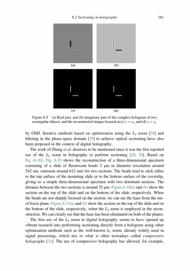
by OSH. Iterative methods based on optimization using the L2 norm [28] andfiltering in the phase-space domain [29] to achieve optical sectioning have alsobeen proposed in the context of digital holography.

The work of Zhang et al. deserves to be mentioned since it was the first reporteduse of the L2 norm in holography to perform sectioning [28, 30]. Based onEq. (6.16), Fig. 6.10 shows the reconstruction of a three-dimensional specimenconsisting of a slide of fluorescent beads 2 μm in diameter (excitation around542 nm, emission around 612 nm) for two sections. The beads tend to stick eitherto the top surface of the mounting slide or to the bottom surface of the coverslip,giving us a simple three-dimensional specimen with two dominant sections. Thedistance between the two sections is around 35 μm. Figure 6.10(a) and (b) show thesection on the top of the slide and on the bottom of the slide, respectively. Whenthe beads are not sharply focused on the section, we can see the haze from the out-of-focus plane. Figure 6.11(a) and (b) show the section on the top of the slide and onthe bottom of the slide, respectively, when the L2 norm is employed in the recon-struction. We can clearly see that the haze has been eliminated on both of the planes.

The first use of the L2 norm in digital holography seems to have opened upvibrant research into performing sectioning directly from a hologram using otheroptimization methods such as the well-known L1 norm, already widely used insignal processing, which ties to what is often nowadays called compressiveholography [31]. The use of compressive holography has allowed, for example,

Figure 6.9 (a) Real part, and (b) imaginary part of the complex hologram of tworectangular objects, and the reconstructed images focused at (c) z¼ z1, and (d) z¼ z2.


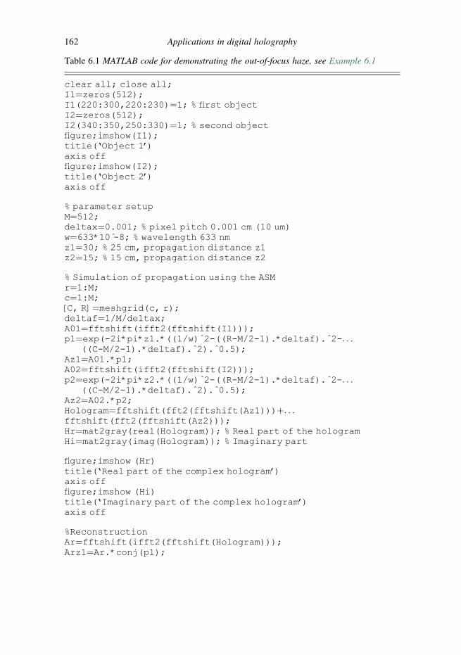
Table 6.1 MATLAB code for demonstrating the out-of-focus haze, see Example 6.1

clear all; close all;I1¼zeros(512);I1(220:300,220:230)¼1; % first objectI2¼zeros(512);I2(340:350,250:330)¼1; % second objectfigure;imshow(I1);title(‘Object 1’)axis offfigure;imshow(I2);title(‘Object 2’)axis off

% parameter setupM¼512;deltax¼0.001; % pixel pitch 0.001 cm (10 um)w¼633*10 -̂8; % wavelength 633 nmz1¼30; % 25 cm, propagation distance z1z2¼15; % 15 cm, propagation distance z2

% Simulation of propagation using the ASMr¼1:M;c¼1:M;[C, R]¼meshgrid(c, r);deltaf¼1/M/deltax;A01¼fftshift(ifft2(fftshift(I1)));p1¼exp(-2i*pi*z1.*((1/w)^2-((R-M/2-1).*deltaf).^2-. . .

((C-M/2-1).*deltaf).^2).^0.5);Az1¼A01.*p1;A02¼fftshift(ifft2(fftshift(I2)));p2¼exp(-2i*pi*z2.*((1/w)^2-((R-M/2-1).*deltaf).^2-. . .

((C-M/2-1).*deltaf).^2).^0.5);Az2¼A02.*p2;Hologram¼fftshift(fft2(fftshift(Az1)))þ. . .fftshift(fft2(fftshift(Az2)));Hr¼mat2gray(real(Hologram)); % Real part of the hologramHi¼mat2gray(imag(Hologram)); % Imaginary part

figure;imshow (Hr)title(‘Real part of the complex hologram’)axis offfigure;imshow (Hi)title(‘Imaginary part of the complex hologram’)axis off

%ReconstructionAr¼fftshift(ifft2(fftshift(Hologram)));Arz1¼Ar.*conj(p1);


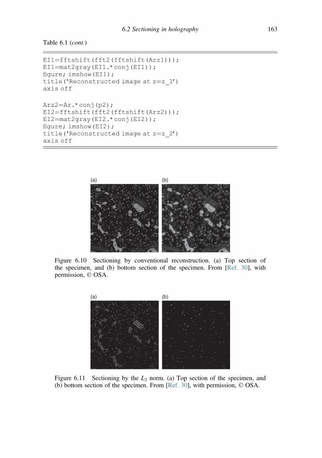
Table 6.1 (cont.)

EI1¼fftshift(fft2(fftshift(Arz1)));EI1¼mat2gray(EI1.*conj(EI1));figure; imshow(EI1);title(‘Reconstructed image at z¼z_1’)axis off

Arz2¼Ar.*conj(p2);EI2¼fftshift(fft2(fftshift(Arz2)));EI2¼mat2gray(EI2.*conj(EI2));figure; imshow(EI2);title(‘Reconstructed image at z¼z_2’)axis off

(a) (b)

Figure 6.10 Sectioning by conventional reconstruction. (a) Top section ofthe specimen, and (b) bottom section of the specimen. From [Ref. 30], withpermission, © OSA.

(a) (b)

Figure 6.11 Sectioning by the L2 norm. (a) Top section of the specimen, and(b) bottom section of the specimen. From [Ref. 30], with permission, © OSA.


rejection of the twin image noise as well as out-of-focus haze for on-axis holo-grams. Most recently, Zhao et al. have proposed an adaptively iterative shrinkage-thresholding algorithm to show that the performance of the algorithm in terms ofsectioning capability is better than that of the L2 norm method [32]. In addition, theproposed algorithm can section well even when using only half of the data of acomplex hologram. It is expected that compressive holography will continue toflourish, for example, with better and faster algorithms, for application tosectioning and to different challenges in holography.

6.3 Phase extraction

One of the most important merits of digital holography is that the phase of thesample can be determined quantitatively. This may find important applications inmicroscopy for biological specimens. We assume that the complex field at thesample plane is ψs¼ jψsjexp( jϕs), which can be retrieved from a complex hologramobtained by digital holography. Consequently, the phase of ψs can be obtained by

ϕw ¼ tan −1 Re ψsf gIm ψsf g

� �: ð6:17Þ

However, the output range of the arctangent is between −π and π. The phaseobtained from Eq. (6.17) is thus wrapped to −π ~ π, as shown in Fig. 6.12. So evenif we have ϕw, the actual phase ϕs can be ϕw þ 2πl for any integer l. To eliminatethis ambiguity, we must extract the continuous phase distribution from thewrapped phase. This procedure is called phase-unwrapping or phase-tracking.

A straightforward method for phase-unwrapping is to detect and compensate forthe phase jump. Here we consider a one-dimensional case as an example. First wecalculate the phase difference between adjacent pixels,

Figure 6.12 The original phase and the wrapped phase.


Δ½n� ¼ ϕw½n�−ϕw½n−1�, ð6:18Þwhere n ¼ 1 ~ N is the pixel index. If Δ[n] is larger than þπ or smaller than −π,then the phase jumps to the lower or upper 2π range, respectively. We must,therefore, add −2π or 2π to the phase of all the following pixels. If none of theabove conditions is valid, the phase value remains unchanged. This procedure canbe done by introducing an intermediate function, g[n],

g½n� ¼g½n−1�−2π for Δ½n� > πg½n−1� þ 2π for Δ½n� < −πg½n−1� otherwise:

8<: ð6:19Þ

By setting the initial conditions ϕuw[1] ¼ ϕw[1], Δ[1] ¼ 0, and g[1] ¼ 0, theunwrapped phase ϕuw[n] can be obtained sequentially by

ϕuw½n� ¼ ϕw½n� þ g½n�: ð6:20Þ

It has also been indicated that Eqs. (6.19) and (6.20) can be expressed using asingle formula as [33]

ϕuw½n� ¼ ϕw½1� þXn−1

m¼1W Δ m½ �f g, ð6:21Þ

where W{�} is the wrapping operator. The wrapping operator can be regarded as anon-linear calculation as

W Δ½m�f g ¼ Δ½m� þ 2πl½m�, ð6:22Þwhere l[m] 2 {. . ., −1, 0, 1, . . .}, i.e., it is a sequence of integers chosen to ensurethat the wrapped function, W{Δ[m]}, is between −π and π. The last term inEq. (6.21) represents a summation of the wrapped phase difference Δ[n]. Equation(6.21) is usually called the Itoh algorithm.

Example 6.2: Phase unwrapping of a wrapped phase map

In this example, a phase function

ϕs x, yð Þ ¼ 15� sinx−225ð Þ2 þ y−200ð Þ2

1000

" #þ x−100ð Þ2 þ y−37ð Þ2

500

" #

is first produced in the range x¼ 0 ~ 256, y¼ 0 ~ 256, and wrapped. The samplingseparation is 0.5, and so the wrapped phase function contains 513 � 513 pixels.The wrapped phase is then unwrapped using the Itoh algorithm.

In this example, we do not write the MATLAB code for implementingEq. (6.21), rather we use directly the MATLAB command unwrap to unwrap the

6.3 Phase extraction 165

wrapped phase function. It should be noted, however, that unwrap only applies to asingle dimension. So we must apply unwrap twice, once for the columns and oncefor the rows. The simulation results are shown in Fig. 6.13, and the MATLABcode is listed in Table 6.2. Figure 6.13(a) shows the original phase ranging from−15 to 150 radians. The wrapped phase, shown in Fig. 6.13(b), ranges from −3.14to 3.14 radians. The unwrapped phase is shown in Fig. 6.13(c), which is nearly thesame as the phase shown in Fig. 6.13(a). Because the phase ϕuw is unwrapped fromsome start point, there is a difference at the start point, ϕuw[n] − ϕs[n], betweenthe unwrapped phase ϕuw and the exact phase ϕs. In the current example of atwo-dimensional phase function, we find the phase difference ϕuw[1,1] − ϕs[1,1] ¼2.92 − 28.05 ¼ −25.13 radians, where we have used the start point at coordinates(x, y) ¼ (0,0) to find the phase difference. Indeed ϕuw[1,1] is the first point when(x, y) ¼ (0,0). We can also use other start points to wrap the phase function butfor this we need to write a code instead of using the MATLAB command. So in

Figure 6.13 (a) The original phase, (b) the wrapped phase, and (c) theunwrapped phase.


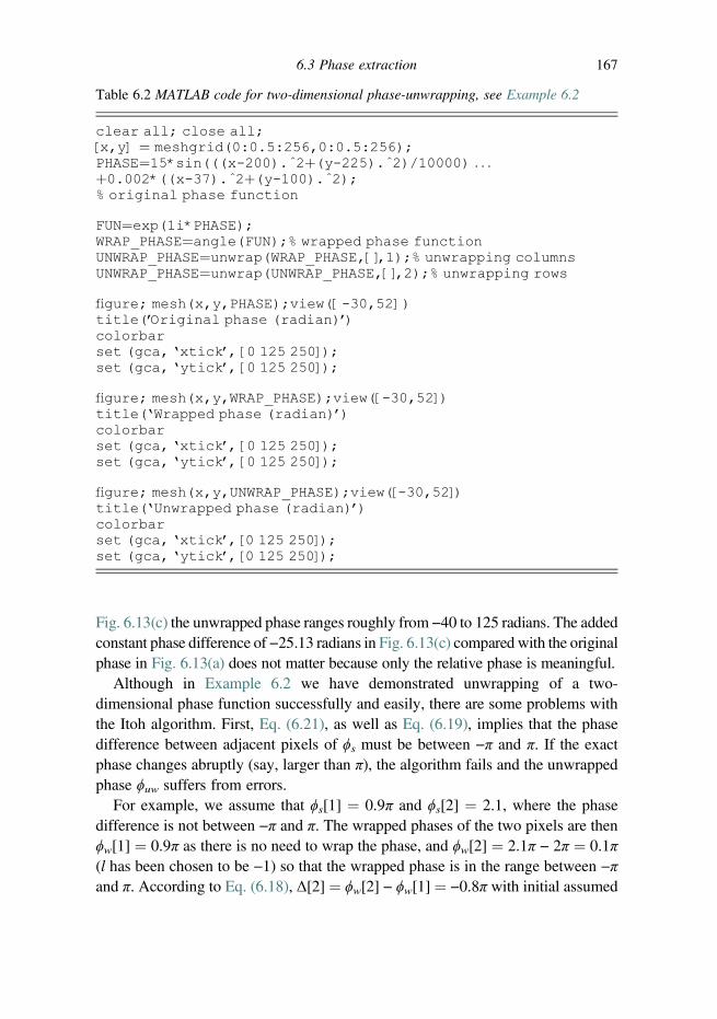
Fig. 6.13(c) the unwrapped phase ranges roughly from −40 to 125 radians. The addedconstant phase difference of −25.13 radians in Fig. 6.13(c) compared with the originalphase in Fig. 6.13(a) does not matter because only the relative phase is meaningful.

Although in Example 6.2 we have demonstrated unwrapping of a two-dimensional phase function successfully and easily, there are some problems withthe Itoh algorithm. First, Eq. (6.21), as well as Eq. (6.19), implies that the phasedifference between adjacent pixels of ϕs must be between −π and π. If the exactphase changes abruptly (say, larger than π), the algorithm fails and the unwrappedphase ϕuw suffers from errors.

For example, we assume that ϕs[1] ¼ 0.9π and ϕs[2] ¼ 2.1, where the phasedifference is not between −π and π. The wrapped phases of the two pixels are thenϕw[1] ¼ 0.9π as there is no need to wrap the phase, and ϕw[2] ¼ 2.1π − 2π ¼ 0.1π(l has been chosen to be −1) so that the wrapped phase is in the range between −πand π. According to Eq. (6.18), Δ[2] ¼ ϕw[2] − ϕw[1] ¼ −0.8π with initial assumed

Table 6.2 MATLAB code for two-dimensional phase-unwrapping, see Example 6.2

clear all; close all;[x,y] ¼ meshgrid(0:0.5:256,0:0.5:256);PHASE¼15*sin(((x-200).^2þ(y-225).^2)/10000) . . .þ0.002*((x-37).^2þ(y-100).^2);% original phase function

FUN¼exp(1i*PHASE);WRAP_PHASE¼angle(FUN);% wrapped phase functionUNWRAP_PHASE¼unwrap(WRAP_PHASE,[],1);% unwrapping columnsUNWRAP_PHASE¼unwrap(UNWRAP_PHASE,[],2);% unwrapping rows

figure; mesh(x,y,PHASE);view([-30,52])title(’Original phase (radian)’)colorbarset (gca,‘xtick’, [0 125 250]);set (gca,‘ytick’, [0 125 250]);

figure; mesh(x,y,WRAP_PHASE);view([-30,52])title(‘Wrapped phase (radian)’)colorbarset (gca,‘xtick’, [0 125 250]);set (gca,‘ytick’, [0 125 250]);

figure; mesh(x,y,UNWRAP_PHASE);view([-30,52])title(‘Unwrapped phase (radian)’)colorbarset (gca,‘xtick’, [0 125 250]);set (gca,‘ytick’, [0 125 250]);

6.3 Phase extraction 167

Δ[1] ¼ 0. Hence according to Eq. (6.19), g[2] ¼ g[1] ¼ 0. We can now, fromEq. (6.20), find ϕuw[1] ¼ ϕw[1] þ g[1] ¼ 0.9π, which is correct. But ϕuw[2] ¼ϕw[2] þ g[2] ¼ 0.1π, which is incorrect.

In addition, in practice the actual acquired phase image is usually contaminatedwith noise. Any noisy pixel may affect the judgment described in Eq. (6.19), andthe phase may be shifted incorrectly up or down. What is worse is that incorrectdetermination of the phase on the nth pixel will propagate to the following (n þ 1,n þ 2,. . .) pixels. Many ingenious, noise-immune unwrapping methods have beenproposed. For example, the noisy pixels are usually detected and excluded from theunwrapping procedure (e.g., [34, 35]).

6.4 Optical contouring and deformation measurement

Because of its fast, non-contact, and three-dimensional imaging ability, digitalholography can be applied to profile measurements or optical contouring. Weassume that the digital hologram is taken using the on-axis, reflection-type digitalholography, as shown in Fig. 6.2. For simplicity, we also assume that complexholograms are obtained by phase shifting or using an off-axis technique. Thecomplex holograms are then reconstructed and unwrapped, and finally the continu-ous phase on the specimen is extracted. In Fig. 6.14, we only show the object beamof the reflection-type microscope-based digital holographic microscope of Fig. 6.2for the following analysis. We consider a plane wave emitting from referenceplane A, which illuminates the specimen and retro-reflects back to plane A. Thephase delay of the light is proportional to the optical path, and thus the unwrappedphase can be expressed as

ϕuw½n� ¼ −2k0dð Þ− −2k0h½n�ð Þ, ð6:23Þ

Figure 6.14 Optical contouring geometry.


where d is the separation between plane A and another reference plane, plane B;h is the height of the specimen measured from plane B. Therefore, the height of thespecimen is given by

h n½ � ¼ ϕuw n½ � þ 2k0d2k0

¼ ϕbuw n½ �2k0

, ð6:24Þ

where ϕbuw½n� is the unwrapped phase found by setting a zero reference phase atplane B. Thus the height separation between 2π phase contouring is

Δhλ ¼ 2π2k0

¼ λ2, ð6:25Þ

which is also called the height sensitivity of the system. Hence we can see that eachcontour is the locus of all points on the surface of the specimen that lie at someconstant height above a reference plane.

Whenever the height difference of the specimen is less than Δhλ/2 ¼ λ/4, wehave ϕbuw½n� ¼ ϕs as the phase difference between adjacent pixels is always lessthan π. In other words, successful unwrapping is achievable if the height variationof a specimen is less than λ/4. However, such height sensitivity in the system beingconsidered is rather small and is sometimes impractical. Hence there is a need tohave a system of large height sensitivity. Two-wavelength contouring, to bediscussed next, is a solution.

6.4.1 Two-wavelength contouring

To extend the range of height measurement without the ambiguity in the procedureof phase-unwrapping, one can use multiple light sources with different wave-lengths to acquire digital holograms sequentially [36–38]. Here we take two-wavelength contouring as an example. We assume that the continuous phasefunctions corresponding to the two wavelengths λ1 and λ2 (λ1 > λ2) are ϕ1s andϕ2s , respectively, where

ϕ1s ½n� ¼ −2k1d½ � þ 2k1h½n�, ð6:26aÞϕ2s ½n� ¼ −2k2d½ � þ 2k2h½n�: ð6:26bÞ

The phase difference is

Δϕs½n� ¼ ϕ2s ½n�−ϕ1s ½n� ¼ 2ðk2−k1Þh½n� þ 2d k1−k2ð Þ: ð6:27ÞOn the right hand side of Eq. (6.27), the second term is a constant phase, and thefirst term can be regarded as the phase delay of light with a synthetic wavelength orequivalent wavelength

6.4 Optical contouring and deformation measurement 169

Λ ¼ λ1λ2λ1−λ2

: ð6:28Þ

By setting λ1 − λ2 ¼ Δλ� λ1, the synthetic wavelength, Λ � λ21=Δλ, is much largerthan λ1. And, according to Eq. (6.25), the height sensitivity is

ΔhΛ ¼ Λ2� λ21

2Δλ: ð6:29Þ

For example, supposing that λ1 ¼ 640.2 nm and λ2 ¼ 640 nm, we will have Δhλ �320 nm and ΔhΛ � 1024 μm. Thus the measurement range of height is signifi-cantly extended.

The two-wavelength procedure begins with two wrapped phase functionsobtained by digital holography,

ϕ1w½n� ¼ W ϕ1s ½n�� ¼ ϕ1s ½n� þ 2πl1½n�, ð6:30aÞ

ϕ2w½n� ¼ W ϕ2s ½n�� ¼ ϕ2s ½n� þ 2πl2½n�, ð6:30bÞ

where l1 and l2 are integers to ensure ϕ1w and ϕ2w are in the �π range, respectively.Note that again according to the Itoh algorithm, ϕ1w or ϕ2w cannot be unwrapped to acorrect unwrapped phase function provided the phase jump between adjacent pixelsof ϕ1s or ϕ

2s is larger than π. The difference between the two wrapped functions is

Δϕw n½ � ¼ ϕ2w n½ �−ϕ1w n½ �¼ ϕ2s ½n�−ϕ1s ½n� þ 2π

l2½n�−l1½n�

�¼ Δϕs½n� þ 2π

l2½n�−l1½n�

�:

ð6:31Þ

Consequently, by unwrapping Δϕw[n], a continuous function Δϕs[n] can beobtained. Similar to Eq. (6.24), the final profile of the specimen can be given by

h n½ � ¼ Δϕs nð Þ2� 2π=Λ

¼ Δϕs nð Þ4π

Λ: ð6:32Þ

Although two-wavelength contouring can efficiently extend the measurement rangeof height, there are two remaining problems. First, the method cannot correctlymeasure structures with a sharp height difference of more than Λ/4 because a phasejump of more than �π occurs at the edges of the element. The other problem is thatthe height error due to the phase error will be amplified in the subtraction process[see Eq. (6.31)]. The two problems can be eliminated together by involving a thirdor more wavelengths [37, 39–41], i.e., multi-wavelength contouring.

Example 6.3: One-dimensional example of two-wavelength optical contouring

In this example, we would like to demonstrate two-wavelength optical contouringin a one-dimensional case. The simulation results are shown in Fig. 6.15, and


Figure 6.15 Two-wavelength optical contouring. (a) Specimen profile; (b)wrapped phase for a single wavelength; (c) unwrapped phase from (b);(d) wrapped phase for a synthetic wavelength; (e) unwrapped phase from (d);(f) recovered profile.

6.4 Optical contouring and deformation measurement 171

the MATLAB code is given in Table 6.3. The profile of a one-dimensionalspecimen is described by

h n½ � ¼ 700−n−201ð Þ21000

μm

in the range n¼ 1 ~ 1000, as shown in Fig. 6.15(a). The two wavelengths involvedin the example are λ1 ¼ 0.650 μm and λ2 ¼ 0.652 μm. Thus the syntheticwavelength is Λ ¼ 212 μm, according to Eq. (6.28). Figure 6.15(b) shows thewrapped phase for λ1. It looks tumultuous because the actual phase differencebetween adjacent pixels exceeds the �π limit. As a result, using the Itoh algorithm,the unwrapped phase shown in Fig. 6.15(c) cannot correctly represent the profile ofthe specimen. Figure 6.15(d) shows the phase difference Δϕw. Note that becauseboth ϕ1w and ϕ2w range between �π, their difference, Δϕw, is between �2π. In otherwords, the difference of l2 and l1, i.e., l2 − l1 in Eq. (6.31), is not always the properparameter for wrapping Δϕs to the �π range. For example, assume that Δϕs[1] ¼0.2π and Δϕs[2] ¼ 0.5π. The phase obtained by Eq. (6.31) is Δϕw[1] ¼ 0.2π, butΔϕw[2] might have wrapped to the range beyond�π because of improper choice ofthe parameter (l2 − l1), and hence Δϕw[2]¼ 0.5π − 2π¼ −1.5π. By setting Δ[1]¼ 0,and g[1] ¼ 0, we can get Δ[2] ¼ Δϕw[2] − Δϕw[1] ¼ −1.5π − 0.2π ¼ −1.7πaccording to Eq. (6.17), and thus g[2] ¼ g[1] þ 2π ¼ 2π according to Eq. (6.18).Finally, from Eq. (6.19) the unwrapped phase will be Δϕuw[2] ¼ Δϕw[2] þ g[2] ¼−1.5π þ 2π ¼ 0.5π, which is the correct phase. So we can still apply theItoh algorithm to unwrap Δϕw, yielding a continuous phase Δϕs, as shown inFig. 6.15(e). Finally, we apply Eq. (6.32) to convert the phase distribution to aprofile function in Fig. 6.15(f), which is identical to Fig. 6.15(a).

6.4.2 Two-illumination contouring

If for some reason we cannot apply two light sources in the holographic system, wecan employ the two-illumination contouring method [42, 43]. Again, the objectarm of the holographic system is highlighted in Fig. 6.16. The geometry is similarto that shown in Fig. 6.14 but now the plane-wave illumination is tilted from thenormal at an angle θ. The light emitting from reference plane A illuminates thespecimen (plane C) and reflects back to plane A again. The phase delay is

ϕ1s ¼ −k0 sin θx−k0 cos θðd−hÞ½ � þ −k0ðd−hÞ½ �, ð6:33Þwhere the first two terms correspond to the optical path from plane A to plane C,and the third term corresponds to the optical path from plane C to plane A. In thesecond recording, the angle of illumination light is changed to θ þ Δθ. The phasedelay becomes


Table 6.3 MATLAB code for demonstrating two-wavelength optical contouring,see Example 6.3

clear all; close all;x¼1:1:1000;h¼ones(1,1000);h¼700-h.*((x-201). 2̂)/1000;h¼h-min(h); % Sample profile in um

L1¼0.650; % first wavelength in umL2¼0.652; % second wavelength in umLs¼L1*L2/(L2-L1); % synthetic wavelength in um

%Phase function for the two wavelengthsPHASE1¼4*pi*h/L1-4*pi*700/L1;PHASE2¼4*pi*h/L2-4*pi*700/L2;FUN1¼exp(1i*PHASE1);WRAP_PHASE1¼angle(FUN1);% wrapped phase function 1FUN2¼exp(1i*PHASE2);WRAP_PHASE2¼angle(FUN2);% wrapped phase function 2

% unwrapping phase function 1UNWRAP_PHASE1¼unwrap(WRAP_PHASE1,[],2);

% difference between two wrapped phase functionsPHASE3¼WRAP_PHASE1-WRAP_PHASE2;

UNWRAP_PHASE3¼unwrap(PHASE3,[],2);% unwrapping synthetic phase function

UNWRAP_PHASE3¼UNWRAP_PHASE3-min(UNWRAP_PHASE3);H¼UNWRAP_PHASE3*Ls/4/pi;% calculate the corresponding height

figure; plot (h);title(’Sample profile’)xlabel(’pixel’);ylabel(’height (\mum )’)figure; plot (WRAP_PHASE1);title(’Wrapped phase 1’)xlabel(’pixel’);ylabel(’Phase (radian )’)figure; plot (UNWRAP_PHASE1);title(’Unwrapped phase 1’)xlabel(’pixel’);ylabel(’Phase (radian )’)figure; plot (PHASE3);title(’Wrapped phase for synthetic wavelength’)xlabel(’pixel’);ylabel(’Phase (radian )’)figure; plot (UNWRAP_PHASE3);title(’Unwrapped phase for synthetic wavelength’)xlabel(’pixel’);ylabel(’Phase (radian )’)figure; plot (H);title(’Recovered profile of the sample’)xlabel(’pixel’);ylabel(’height (\mum )’)

ϕ2s ¼ −k0 sin θ þ Δθð Þx−k0 cos θ þ Δθð Þðd−hÞ½ � þ −k0ðd−hÞ½ �: ð6:34ÞThe difference of the two phase functions is thus

Δϕs ¼ ϕ2s−ϕ1s ¼ 2k0 sin

Δθ2

sin θ þ Δθ2

� ðd−hÞ− cos θ þ Δθ

2

� x

� �ð6:35Þ

by applying two identities

sin α− sin β ¼ 2 cos

�αþ β2

cos

�α−β2

,

cos α− cos β ¼ −2 sin

�αþ β2

sin

�α−β2

:

The x-dependent term in Eq. (6.35) is a familiar carrier term as in a carrier-frequency hologram [see Eq. (3.5b)] and its phase term (the first term of the righthand side of the equation) can be extracted to yield a height-dependent phase as

Δϕs0 ¼ 2k0 sin

Δθ2

sin θ þ Δθ2

� ðd−hÞ: ð6:36Þ

Therefore, the specimen height can be retrieved by

h ¼ d−Δϕs

0

2k0 sinΔθ2

sin θ þ Δθ2

� : ð6:37Þ

Accordingly, the height sensitivity corresponding to 2π contouring is

Δh ¼ λ

2 sinΔθ2

sin θ þ Δθ2

� � λΔθ sin θ

ð6:38Þ

for a small tilt angle Δθ. For example, for λ ¼ 640 nm, θ ¼ 20, and Δθ ¼ 0.05,the height sensitivity is Δh ¼ 2144 μm.

Figure 6.16 Two-illumination contouring geometry.


6.4.3 Deformation measurement

Sometimes, such as measurement of the Young modulus of a material, it is theprofile deformation instead of the whole profile which is of interest. Deformationmeasurement can also be realized using the setup shown in Fig. 6.16 [44]. First ahologram corresponding to the original profile is recorded. The retrieved phasefunction is described by Eq. (6.33). The specimen undergoes a small deformation,and a second hologram is recorded. The retrieved phase function of the secondhologram is

ϕ2s ¼ −k0 sin θx−k0 cos θðd−h−δhÞ½ � þ −k0ðd−h−δhÞ½ �, ð6:39Þwhere δh denotes the height deformation of the specimen. As a result, the differ-ence between the first and second phase functions is

Δϕs ¼ ϕ2s−ϕ1s ¼ k0ð1þ cos θÞδh: ð6:40Þ

The height deformation is thus given by

δh ¼ Δϕsk0 1þ cos θð Þ : ð6:41Þ

In two-illumination contouring, some portions of the specimen may be shadowedbecause the illumination light is tilted. This problem together with any additivenoise can be eliminated by applying more than two illuminations with differentillumination directions [45, 46].

Problems

6.1 A CCD imager contains 1000 � 1000 pixels with a pixel pitch of 6 μm, and itis used in spherical-reference-based DHM. Find a combination of (z0, zr),where the distances z0 and zr are defined in Fig. 6.5(a), so that the acquiredhologram is well sampled and the lateral resolution in the object space is betterthan 1.2 μm. Assume that phase-shifting procedures have been applied toextract a complex hologram and the wavelength used is λ0 ¼ 0.6 μm.

6.2 The CCD described in Problem 6.1 is applied in Fourier-based DHM. Find theobject distance z0 and the size of reconstructed field when a lateral resolutionbetter than 1.2 μm is required. Assume that phase-shifting procedures havebeen applied to extract a complex hologram and the wavelength used isλ0 ¼ 0.6 μm.

References

1. D. Garbor, A new microscopic principle, Nature 161, 777–778 (1948).2. E. N. Leith, and J. Upatnieks, Microscopy by wavefront reconstruction, Journal of the

Optical Society of America 55, 569 (1965).

References 175

3. T. Zhang, and I. Yamaguchi, Three-dimensional microscopy with phase-shiftingdigital holography, Optics Letters 23, 1221–1223 (1998).

4. E. Cuche, P. Marquet, and C. Depeursinge, Simultaneous amplitude-contrast andquantitative phase-contrast microscopy by numerical reconstruction of Fresnel off-axis holograms, Applied Optics 38, 6994–7001 (1999).

5. P. Ferraro, S. De Nicola, A. Finizio, G. Coppola, S. Grilli, C. Magro, and G. Pierattini,Compensation of the inherent wave front curvature in digital holographic coherentmicroscopy for quantitative phase-contrast imaging, Applied Optics 42, 1938–1946(2003).

6. T. Colomb, E. Cuche, F. Charrière, J. Kühn, N. Aspert, F. Montfort, P. Marquet,and C. Depeursinge, Automatic procedure for aberration compensation in digitalholographic microscopy and applications to specimen shape compensation, AppliedOptics 45, 851–863 (2006).

7. K. J. Chalut, W. J. Brown, and A. Wax, Quantitative phase microscopy with asyn-chronous digital holography, Optics Express 15, 3047–3052 (2007).

8. J. W. Kang, and C. K. Hong, Phase-contrast microscopy by in-line phase-shiftingdigital holography: shape measurement of a titanium pattern with nanometer axialresolution, Optical Engineering 46, 040506 (2007).

9. W. S. Haddad, D. Cullen, J. C. Solem, J. W. Longworth, A. McPherson, K. Boyer,and C. K. Rhodes, Fourier-transform holographic microscope, Applied Optics 31,4973–4978 (1992).

10. C. Wagner, S. Seebacher, W. Osten, and W. Jüptner, Digital recording and numericalreconstruction of lensless Fourier holograms in optical metrology, Applied Optics 38,4812–4820 (1999).

11. D. Dirksen, H. Droste, B. Kemper, H. Deleré, M. Deiwick, H. H. Scheld, and G. vonBally, Lensless Fourier holography for digital holographic interferometry onbiological samples, Optics and Lasers in Engineering 36, 241–249 (2001).

12. G. Pedrini, and H. J. Tiziani, Short-coherence digital microscopy by use of a lenslessholographic imaging system, Applied Optics 41, 4489–4496 (2002).

13. M. Sebesta, and M. Gustafsson, Object characterization with refractometric digital-Fourier holography, Optics Letters 30, 471–473 (2005).

14. L. Granero, V. Micó, Z. Zalevsky, and J. García, Superresolution imaging methodusing phase-shifting digital lensless Fourier holography, Optics Express 17, 15008–15022 (2009).

15. I. Yamaguchi, J.-I. Kato, S. Ohta, and J. Mizuno, Image formation in phase-shiftingdigital holography and applications to microscopy, Applied Optics 40, 6177–6186(2001).

16. J. W. Goodman, Introduction to Fourier Optics (McGraw-Hill, New York, 2005),pp. 108–115.

17. T. Colomb, J. Kühn, F. Charrière, C. Depeursinge, P. Marquet, and N. Aspert, Totalaberrations compensation in digital holographic microscopy with a referenceconjugated hologram, Optics Express 14, 4300–4306 (2006).

18. J. Di, J. Zhao, W. Sun, H. Jiang, and X. Yan, Phase aberration compensation of digitalholographic microscopy based on least squares surface fitting, Optics Communications282, 3873–3877 (2009).

19. V. Micó, J. García, Z. Zalevsky, and B. Javidi, Phase-shifting Gabor holography,Optics Letters 34, 1492–1494 (2009).

20. V. Micó, L. Granero, Z. Zalevsky, and J. García, Superresolved phase-shiftingGabor holography by CCD shift, Journal of Optics A, Pure and Applied Optics 11,125408 (2009).


21. W. Xu, M. H. Jericho, H. J. Kreuzer, and I. A. Meinertzhagen, Tracking particles in fourdimensions with in-line holographic microscopy, Optics Letters 28, 164–166 (2003).

22. J. Garcia-Sucerquia, W. Xu, S. K. Jericho, P. Klages, M. H. Jericho, and H. J. Kreuzer,Digital in-line holographic microscopy, Applied Optics 45, 836–850 (2006).

23. W. Xu, M. H. Jericho, I. A. Meinertzhagen, and H. J. Kreuzer, Digital in-lineholography of microspheres, Applied Optics 41, 5367–5375 (2002).

24. G. Indebetouw, A posteriori quasi-sectioning of the three-dimensional reconstructionsof scanning holographic microscopy, Journal of the Optical Society of America 23,2657–2661 (2006).

25. A. Anand, and S. Vijay Raj, Sectioning of amplitude images in digital holography,Measurement Science and Technology 17, 75–78 (2006).

26. W.-C. Chien, D. S. Dilworth, E. Liu, and E. N. Leith, Synthetic-aperture chirpconfocal imaging, Applied Optics 45, 501–510 (2006).

27. T. Kim, Optical sectioning by optical scanning holography and a Wiener filter,Applied Optics 45, 872–879 (2006).

28. X. Zhang, E. Y. Lam, and T.-C. Poon, Reconstruction of sectional images in holog-raphy using inverse imaging, Optics Express 16, 17215–17226 (2008).

29. H. Kim, S.-W. Min, B. Lee, and T.-C. Poon, Optical sectioning for optical scanningholography using phase-space filtering with Wigner distribution functions, AppliedOptics 47, D164–D175 (2008).

30. E. Y. Lam, X. Zhang, H. Vo, T.-C. Poon, and G. Indebetouw, Three-dimensionalmicroscopy and sectional image reconstruction using optical scanning holography,Applied Optics 48, H113–H119 (2009).

31. J. Hahn, S. Lim, K. Choi, R. Horisaki, and D. J. Brady, Video-rate compressiveholographic microscopic tomography, Optics Express 19, 7289–7298 (2011).

32. F. Zhao, X. Qu, X. Zhang, T.-C. Poon, T. Kim, Y. S. Kim, and J. Liang, Solvinginverse problems for optical scanning holography using an adaptively iterativeshrinkage-thresholding algorithm, Optics Express 20, 5942–5954 (2012).

33. K. Itoh, Analysis of the phase unwrapping algorithm, Applied Optics 21, 2470–2470(1982).

34. D. C. Ghiglia, and M. D. Pritt, Two-Dimensional Phase Unwrapping: Theory, Algo-rithms, and Software (John Wiley & Sons, New York, 1998).

35. T. R. Judge, and P. J. Bryanston-Cross, A review of phase unwrapping techniques infringe analysis, Optics and Lasers in Engineering 21, 199–239 (1994).

36. I. Yamaguchi, T. Ida, M. Yokota, and K. Yamashita, Surface shape measurement byphase-shifting digital holography with a wavelength shift, Applied Optics 45, 7610–7616 (2006).

37. D. Parshall, and M. K. Kim, Digital holographic microscopy with dual-wavelengthphase unwrapping, Applied Optics 45, 451–459 (2006).

38. G. Pedrini, P. Fröning, H. J. Tiziani, and M. E. Gusev, Pulsed digital holographyfor high-speed contouring that uses a two-wavelength method, Applied Optics 38,3460–3467 (1999).

39. C. Wagner, W. Osten, and S. Seebacher, Direct shape measurement by digitalwavefront reconstruction and multiwavelength contouring, Optical Engineering 39,79–85 (2000).

40. A. Wada, M. Kato, and Y. Ishii, Multiple-wavelength digital holographic interfer-ometry using tunable laser diodes, Applied Optics 47, 2053–2060 (2008).

41. A. Wada, M. Kato, and Y. Ishii, Large step-height measurements using multiple-wavelength holographic interferometry with tunable laser diodes, Journal of theOptical Society of America A 25, 3013–3020 (2008).

References 177

42. I. Yamaguchi, S. Ohta, and J.-I. Kato, Surface contouring by phase-shifting digitalholography, Optics and Lasers in Engineering 36, 417–428 (2001).

43. D. Velásquez Prieto, and J. Garcia-Sucerquia, Three-dimensional surface contouringof macroscopic objects by means of phase-difference images, Applied Optics 45,6381–6387 (2006).

44. I. Yamaguchi, J.-I. Kato, and H. Matsuzaki, Measurement of surface shape anddeformation by phase-shifting image digital holography, Optical Engineering 42,1267–1271 (2003).

45. S. Seebacher, T. Baumbach, W. Osten, and W. P. O. Jueptner, Combined 3D-shapeand deformation analysis of small objects using coherent optical techniques on thebasis of digital holography, SPIE Proceedings 4101, 510–521 (2000).

46. S. M. Solís, F. M. Santoyo, and M. D. S. Hernández-Montes, 3D displacementmeasurements of the tympanic membrane with digital holographic interferometry,Optics Express 20, 5613–5621 (2012).


7

Computer-generated holography

Computer-generated holography deals with the methods used for the generation ofholograms digitally. The hologram can be subsequently printed on a film or loadedonto a spatial light modulator (SLM) for holographic reconstruction. Computer-generated holograms (CGHs) have the advantage that the three-dimensionalobjects do not have to exist in the real world. In other words, the objectswhich one wants to display can be fictitious. For generating CGHs, differentcalculation methods have been developed for fitting various display devices andreconstruction methods. In this chapter, we first discuss some of the historicalmethods of generating computer-generated holograms and then we describe somemodern approaches for fast calculations as well as ways to process holographicinformation. Finally, we discuss three-dimensional holographic display andaddress some of the issues involving display with SLMs.

7.1 The detour-phase hologram

In the early history of computer-generated holography, neither gray-tone plottersnor SLMs were available. Therefore, it was necessary to reconstruct aquality image from a binary, amplitude-only hologram. The first such CGH wasthe Fourier-type detour-phase hologram, which was invented by Brown andLohmann [1, 2].

Figure 7.1 shows the setup for reconstructing a Fourier hologram through aFourier transform lens of focal length f. We are not concerned with the zeroth-orderlight and the twin image in the following discussion. As we know, the hologramH(x, y) and the complex amplitude of the reconstructed image ψ(x, y) are related by

ψðx, yÞ ¼ F H x,yð Þψr x,yð Þf gkx ¼ k0x

f , ky ¼ k0yf, ð7:1Þ

179

where ψr (x, y) ¼ exp (−jk0 sinθx) denotes the complex amplitude of a plane wavereconstruction light, and θ is the tilt angle.

In general, the hologram is a complex function, that is H(x, y) ¼ a(x, y)exp[–jϕ(x, y)], where a(x, y) and ϕ(x, y) are the modulus and the phase ofthe hologram, respectively. Hence the goal is to devise a binary (opaque ortransparent) amplitude pattern Hb(x, y) to approximate the complex hologramH(x, y). This seems a formidable problem, but if our concern is limited to awindow of size dx � dy at the reconstruction plane, it is possible to find Hb(x, y)such that

F Hb x, yð Þψr x, yð Þf g � F H x, yð Þψr x, yð Þf g ð7:2Þwithin the window.

First, the area of the hologram is divided into an array of unit cells, and the sizeof each cell is w � w, as shown in Fig. 7.2. For the complex hologram H(x, y),suppose that both a(x, y) and ϕ(x, y) vary slowly within any cell; the cells can thenbe replaced by an array of point sources, yielding a sampled complex hologram as

Hsðx, yÞ ¼Xm, n

amne−jϕmn � δ x − xm, y − ynð Þ, ð7:3Þ

where (m, n) indexes the cell centered at xm ¼ mw, yn ¼ nw; amn ¼ a(xm, yn) andϕmn ¼ ϕ(xm, yn). Under the illumination of a tilted plane wave, each point source inthe sampled hologram produces a plane wave on the reconstruction plane, giving acomplex field in the reconstruction plane as

ψs x, yð Þ ¼ F expð−jk0 sin θxÞHs x,yð Þf gkx ¼ k0x

f , ky ¼ k0yf¼Xm, n

amne−jϕmne−jk0 sin θxme

hjk0f ðxmxþ ynyÞ

i:

ð7:4Þ

Figure 7.1 Reconstruction scheme for the detour-phase hologram.

180 Computer-generated holography

We can eliminate the effect of the unwanted phase term exp (−jk0 sinθxm) inEq. (7.4) by designing the width of the unit cell to be

w ¼ 2πℓk0 sin θ

, ℓ 2 1, 2, 3 . . . ð7:5Þ

as exp(−j2πℓm) ¼ 1, yielding

ψs x, yð Þ ¼Xm, n

amne−jϕmne

hjk0f xmxþ ynyð Þ

i, ð7:6Þ

which represents the approximation of a Fourier transform of the sampled complexhologram amne−jϕmn :

Figure 7.2 Cell description of (a) a complex hologram, and (b) a detour-phasebinary hologram.

7.1 The detour-phase hologram 181

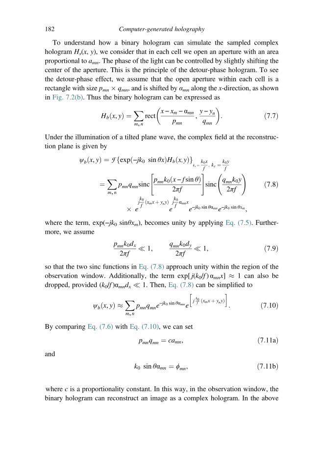
To understand how a binary hologram can simulate the sampled complexhologram Hs(x, y), we consider that in each cell we open an aperture with an areaproportional to amn. The phase of the light can be controlled by slightly shifting thecenter of the aperture. This is the principle of the detour-phase hologram. To seethe detour-phase effect, we assume that the open aperture within each cell is arectangle with size pmn � qmn, and is shifted by αmn along the x-direction, as shownin Fig. 7.2(b). Thus the binary hologram can be expressed as

Hb x, yð Þ ¼Xm, n

rectx − xm − αmn

pmn,y − ynqmn

� �: ð7:7Þ

Under the illumination of a tilted plane wave, the complex field at the reconstruc-tion plane is given by

ψb x, yð Þ ¼ F expð−jk0 sin θxÞHb x,yð Þf gkx ¼

k0x

f, ky ¼ k0y

f

¼Xm, n

pmnqmnsincpmnk0 x − f sin θð Þ

2πf

" #sinc

qmnk0y

2πf

!

� ejk0f

xmxþ ynyð Þejk0fαmnx

e−jk0 sin θαmne−jk0 sin θxm ,

ð7:8Þ

where the term, exp(−jk0 sinθxm), becomes unity by applying Eq. (7.5). Further-more, we assume

pmnk0dx2πf

� 1,qmnk0dy2πf

� 1, ð7:9Þ

so that the two sinc functions in Eq. (7.8) approach unity within the region of theobservation window. Additionally, the term exp[ j(k0/f ) αmnx] � 1 can also bedropped, provided (k0/f )αmndx � 1. Then, Eq. (7.8) can be simplified to

ψb x, yð Þ �Xm, n

pmnqmne−jk0 sin θαmne

hjk0f xmx þ ynyð Þ

i: ð7:10Þ

By comparing Eq. (7.6) with Eq. (7.10), we can set

pmnqmn ¼ camn, ð7:11aÞand

k0 sin θαmn ¼ ϕmn, ð7:11bÞ

where c is a proportionality constant. In this way, in the observation window, thebinary hologram can reconstruct an image as a complex hologram. In the above


analysis, the aperture in the cell is rectangular, but it can be any shape, such ascircular, with an area proportional to amn. From Eqs. (7.5) and (7.11b), we candetermine the shift of the aperture within each cell by

αmn ¼ ϕmnk0 sin θ

¼ ϕmn2π

w

ℓ: ð7:12Þ

Because ϕmn is wrapped between π and −π, the range of αmn is within �w/2ℓ.

Example 7.1: Generation of a detour-phase CGH

In this example we will generate a detour-phase CGH. In the detour-phasehologram, the structure in a cell must be controlled. So we use 16 � 16 pixels toconstruct a cell, and the hologram consists of 64 � 64 cells. So there is a totalof 1024 � 1024 pixels in the hologram. The 64 � 64-pixel object is shown inFig. 7.3(a). It is noted that we must attach a random-phase mask against the objectin order to broaden its spectrum. Otherwise, most of the energy will concentrate inthe zeroth-order beam and the effective dynamic range of the produced hologramwill be reduced. The random-phase-added object is transformed to the Fourierdomain also with 64 � 64 pixels. The value of each pixel is complex, and will

Figure 7.3 (a) Original object, (b) detour-phase hologram of (a), (c) recon-structed image, and (d) enlarged reconstructed image with selected diffractedorder from (c).

7.1 The detour-phase hologram 183

Table 7.1 MATLAB code for generating a detour-phase CGH, see Example 7.1

clear all; close all;I¼imread(’DH64.bmp’, ’bmp’);% please prepare a 8 bit, 64x64 pixels input image% otherwise the code must adjusted accordingly

I¼double(I);figure; imshow(abs(I));title(’Original object’)

PH¼rand([64,64]);I¼I.*exp(2i*pi*PH);% add a random phase to the object

FTS¼fftshift(ifft2(fftshift(I)));A¼abs(FTS);figure;imshow(mat2gray(A));title(’Object spectrum’)

A¼A./max(max(A))*15;A¼round(A);% The amplitude is divided into 16 levelsB¼angle(conj(FTS));B¼B-min(min(B));B¼B./max(max(B))*7;B¼round(B);% The phase is divided into 8 levelsH¼zeros(1024);

for m¼1:64;for n¼1:64;

P¼zeros(16);a¼A(m,n);b¼B(m,n);c¼fix(a/2);d¼rem(a,2);P(9-c:8þcþd,(1þb):(9þb))¼1;H(16*(m-1)þ1:16*(m-1)þ16,16*(n-1)þ1:16*(n-1)þ16)¼P;

endend

figure; imshow(H)title(’Detour-phase CGH’)imwrite(H, ’1AA.jpg’,’jpg’)

%Reconstruction (FFT)R¼fftshift(ifft2(fftshift(H)));figure; imshow(100.*mat2gray(abs(R)));title(’Reconstructed image’)


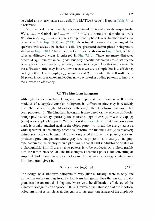
be coded to a binary pattern as a cell. The MATLAB code is listed in Table 7.1 asa reference.

First, the modulus and the phase are quantized to 16 and 8 levels, respectively.We set pmn ¼ 9 pixels, and qmn ¼ 1 ~ 16 pixels to represent 16 modulus levels.We also select αmn ¼ −4 ~ 3 pixels to represent 8 phase levels. In other words, weselect ℓ ¼ 2 in Eqs. (7.5) and (7.12). By using this setup, the opening of theaperture will always be inside a cell. The produced detour-phase hologram isshown in Fig. 7.3(b). The reconstructed image is shown in Fig. 7.3(c), while aselected diffracted order is enlarged in Fig. 7.3(d). There are many diffractedorders of light due to the cell grids, but only specific diffracted orders satisfy theassumptions in our analysis, resulting in quality images. Note that in the examplethe diffraction efficiency is very low because we use a simple but low-efficiencycoding pattern. For example, pmn cannot exceed 9 pixels while the cell width, w, is16 pixels in our present example. One may devise other coding patterns to improvethe diffraction efficiency.

7.2 The kinoform hologram

Although the detour-phase hologram can represent the phase as well as themodulus of a sampled complex hologram, its diffraction efficiency is relativelylow. To achieve high diffraction efficiency, the kinoform hologram hasbeen proposed [3]. The kinoform hologram is also based on the scheme of Fourierholography. Generally speaking, the Fourier hologram H(x, y) ¼ a(x, y) exp[−jϕ(x, y)] is a complex hologram. We mentioned in Example 7.1 that a random-phasemask is usually attached against the object pattern to spread the energy across awide spectrum. If the energy spread is uniform, the modulus a(x, y) is relativelyunimportant and can be ignored. So we only need to extract the phase ϕ(x, y) andproduce a gray-tone pattern whose gray-level is proportional to ϕ(x, y). The gray-tone pattern can be displayed on a phase-only spatial light modulator or printed ona photographic film. If a gray-tone pattern is to be produced on a photographicfilm, the film is bleached and the bleaching is a chemical process for converting anamplitude hologram into a phase hologram. In this way, we can generate a kino-form hologram given by

Hp x, yð Þ ¼ exp −jϕðx, yÞ½ �: ð7:13ÞThe design of a kinoform hologram is very simple. Ideally, there is only onediffraction order emitting from the kinoform hologram. Thus the kinoform holo-gram can be an on-axis hologram. Moreover, the diffraction efficiency of thekinoform hologram can approach 100%. However, the fabrication of the kinoformhologram is not as simple as its design. First, the gray-tone fringes of the amplitude

7.2 The kinoform hologram 185

hologram must be plotted correctly. Second, the amplitude transmittance must beconverted to phase retardation linearly. And finally, the phase retardation mustbe precise in the range 0 ~ 2π (integral multiples of 2π radians are subtracted forany point in the hologram to be within 2π radians). Otherwise, the diffractionefficiency drops and the zeroth-order light appears. In computer-generated holog-raphy, kinoform holograms are easy to generate as we simply extract the phaseinformation from the computed complex field of an object and display on a phase-only SLM. To demonstrate the principle, we use a pattern shown in Fig. 7.4(a) asthe input. We also attach a random-phase mask against the pattern. The random-phase mask is shown in Fig. 7.4(b). The phase of the spectrum of the object withthe random-phase mask is shown in Fig. 7.4(c). Although the energy spreads outby the random phase in the spectrum domain, the spectrum is locally non-uniform.While we still assume a uniform modulus to generate a kinoform hologram,the corresponding reconstructed image is shown in Fig. 7.4(d). The MATLABcode is listed in Table 7.2. There is notable speckle noise in the reconstructedimage. This is a consequence of the non-uniform modulus of the spectrum.The problem can be avoided by using specific object patterns. Alternatively,optimization procedures, such as the iterative Fourier transform algorithm (Section7.3), can be applied to improve the image quality [4, 5].

Figure 7.4 (a) Original object, (b) random-phase mask with phase rangingfrom −π to π, (c) spectrum of the object with the random-phase mask, and(d) reconstructed image of the kinoform (phase-only) hologram.


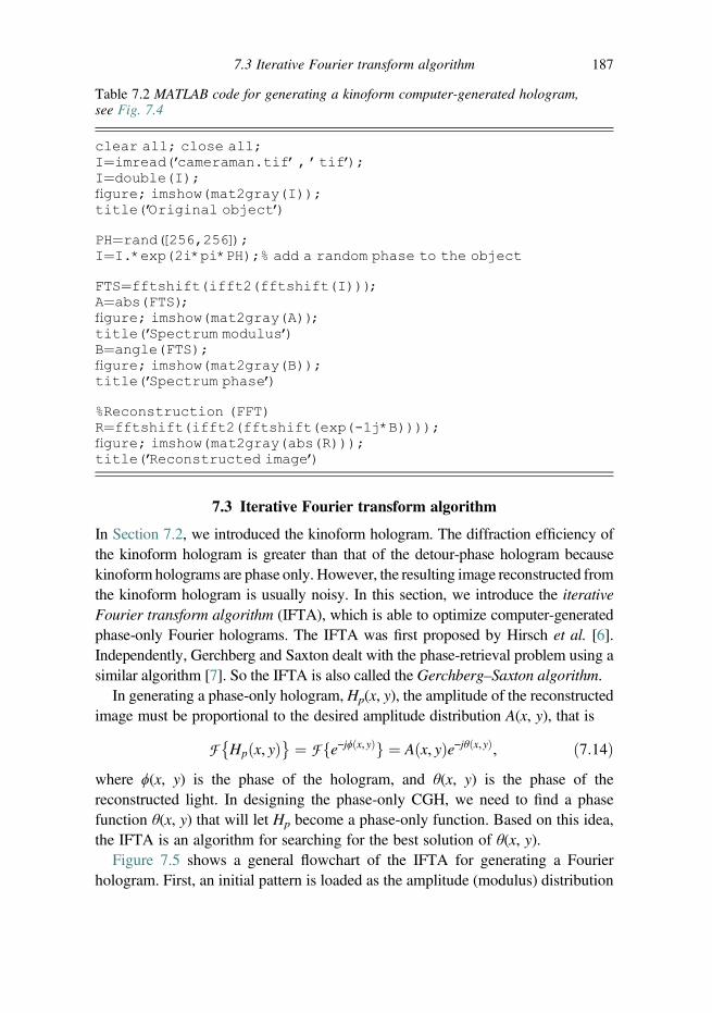
7.3 Iterative Fourier transform algorithm

In Section 7.2, we introduced the kinoform hologram. The diffraction efficiency ofthe kinoform hologram is greater than that of the detour-phase hologram becausekinoform holograms are phase only. However, the resulting image reconstructed fromthe kinoform hologram is usually noisy. In this section, we introduce the iterativeFourier transform algorithm (IFTA), which is able to optimize computer-generatedphase-only Fourier holograms. The IFTA was first proposed by Hirsch et al. [6].Independently, Gerchberg and Saxton dealt with the phase-retrieval problem using asimilar algorithm [7]. So the IFTA is also called the Gerchberg–Saxton algorithm.

In generating a phase-only hologram,Hp(x, y), the amplitude of the reconstructedimage must be proportional to the desired amplitude distribution A(x, y), that is

F Hp x, yð Þ� � ¼ F fe−jϕ x,yð Þg ¼ Aðx, yÞe−jθðx,yÞ, ð7:14Þwhere ϕ(x, y) is the phase of the hologram, and θ(x, y) is the phase of thereconstructed light. In designing the phase-only CGH, we need to find a phasefunction θ(x, y) that will let Hp become a phase-only function. Based on this idea,the IFTA is an algorithm for searching for the best solution of θ(x, y).

Figure 7.5 shows a general flowchart of the IFTA for generating a Fourierhologram. First, an initial pattern is loaded as the amplitude (modulus) distribution

Table 7.2 MATLAB code for generating a kinoform computer-generated hologram,see Fig. 7.4

clear all; close all;I¼imread(’cameraman.tif’, ’tif’);I¼double(I);figure; imshow(mat2gray(I));title(’Original object’)

PH¼rand([256,256]);I¼I.*exp(2i*pi*PH);% add a random phase to the object

FTS¼fftshift(ifft2(fftshift(I)));A¼abs(FTS);figure; imshow(mat2gray(A));title(’Spectrum modulus’)B¼angle(FTS);figure; imshow(mat2gray(B));title(’Spectrum phase’)

%Reconstruction (FFT)R¼fftshift(ifft2(fftshift(exp(-1j*B))));figure; imshow(mat2gray(abs(R)));title(’Reconstructed image’)

7.3 Iterative Fourier transform algorithm 187

A(x, y) of the target reconstructed field. If desired, one can also apply a phase maskon the input pattern as the initial field. The initial field is then Fourier transformedto the spectrum domain. The spectrum is modified according to a constraint. In ourproblem the constraint is that the spectrum modulus must be uniform. So we set thespectrum modulus to become unity without altering its phase. The modifiedspectrum is transformed back to the spatial domain. We then apply a constrainton the resulting field in the spatial domain, thereby obtaining a new field. In our

Figure 7.5 Flowchart of the IFTA.


problem the constraint in the spatial domain is the given modulus distribution,A(x, y). So we enforce the modulus of the field to be A(x, y) without alteringits phase. The resulting field is then regarded as the initial field in the next iteration.Iterations are repeated until the goal (e.g., iteration number) is achieved.

When using the IFTA, it is important to hold sufficient degrees of freedom.If the constraint in either the spatial domain or the spectrum domain is too severe,there will be no satisfactory solution. If the constraint is proper, the resulting fieldwill converge to an optimized solution. Note that the IFTA only searches for asmall region of the phase-function set. For example, for a 512 � 512-pixel phasefunction with 256 phase levels, there are a total of 256512�512 phase functions.Thus, the solution found by the IFTA may be only locally optimized, i.e., it is thebest solution within the searched region, but not a globally optimized solution(the best solution in the complete set). Additional algorithms must be includedin the IFTA to search for a globally optimized solution [8, 9].

Example 7.2: Phase-only Fourier hologram by IFTA

In this example, we use the image shown in Fig. 7.4(a) as the initial pattern. TheMATLAB code for the IFTA is listed in Table 7.3. First, the initial input image istransformed to the spectrum domain, and the phase spectrum is extracted andtransformed back to the spatial domain. To monitor the quality of the resultingreconstructed image of the hologram, we measure the root-mean-square error(RMSE), which is defined as

RMSE ¼ 1MN

Xm,n

�jψðm,nÞj−Aðm,nÞ�2( )0:5

, ð7:15Þ

where A(m, n) is the target image, ψ(m, n) is the evaluated field, (m, n) are thesampling indices, andM andN are the sampling numbers along the x-axis and y-axis,respectively. Figure 7.6(a) shows the RMSE as a function of the iteration number.In the example, the total number of iterations is 100. The error decreases graduallyas the number of iterations increases. The resulting reconstructed image after 100 iter-ations is shown in Fig. 7.6(b). Note that it is comparable to Fig. 7.4(a).

7.4 Modern approach for fast calculations and holographicinformation processing

7.4.1 Modern approach for fast calculations

Holography is a technique for recording thewavefront of a three-dimensional scene ona two-dimensional recording device such as a photographic film or CCD camera.A few decades ago, the recording process could only be accomplished by opticalmeans by mixing the object wave with a reference wave, and recording the resulting

7.4 Calculations and holographic information processing 189

Table 7.3 MATLAB code for generating a phase-only Fourier hologram using the IFTA,see Example 7.2

clear all; close all;I¼imread(’cameraman.tif’, ’tif’);I¼double(I);I¼I./max(max(I));avg1¼mean(mean(I));figure;imshow(mat2gray(I));title(’Original object’);figure;axis([0,101,0,1]);xlabel(’Number of iterations’)ylabel(’RMSE’)hold onI1¼I;for n¼1:100; % iterations to optimize the phase hologram

H¼fftshift(fft2(fftshift(I1)));I2¼fftshift(ifft2(fftshift(exp(1j.*angle(H)))));avg2¼mean(mean(abs(I2)));I2¼(I2./avg2).*avg1;rmse¼(mean(mean((abs(I2)-I). 2̂))) 0̂.5;plot(n,rmse, ’o’);pause(0.3); % To see the error in each iteration.I1¼I.*exp(1j*angle(I2));endhold offI2¼I2./max(max(abs(I2)));figure;imshow(abs(I2));title(’Reconstructed image’)

Figure 7.6 (a) RMSE as a function of iteration number, (b) reconstructed imageafter 100 iterations.


fringe pattern on a recording device. With the rapid advancement of computingtechnologies in recent years, the optical hologram formation process can now besimulated by numerical means. Such an approach, commonly referred to ascomputer-generated holography [1], computes the diffraction pattern emitted from athree-dimensional object and adds a referencewave to produce a digital hologram. Thehologram can be displayed on electronic addressable devices (e.g., spatial lightmodulator) [10], or printed with laser [11] or fringe printers [12], and subsequentlyreconstructed to give a three-dimensional scene upon suitable illumination. Digitalholography is likely to be a promising solution in the next generation of three-dimensional display. At the same time, such optimism is masked by a number ofpractical problems which are difficult to solve in the foreseeable future. Many of theseproblems can be traced back to the fine pixel size of a hologram, which is of the orderof the wavelength of light. For example, a small 10 mm � 10 mm hologram with asquare pixel size of 5 μm � 5 μm, is made up of over 4 � 106 points, which is abouttwo times more than the number of pixels in a domestic high-definition television of1920 � 1080 pixels. One can easily imagine the formidable amount of computationassociated with the generation and processing of a large hologram digitally. In thissection, we will first discuss research based on a modern framework of digitalholography known as the wavefront recording plane (WRP), which is generalized asthe virtual diffraction plane (VDP), if digital processing of holographic data is desired.We will then cover the framework based on the VDP in the subsequent section.

The concept and theory of the WRP were first proposed by a group of research-ers into fast generation of digital holograms [13, 14]. Traditional approaches(for example, [15–17]) aimed at enhancing the speed of generating a hologramdirectly from an object scene, whereas the WRP approach considers a hypotheticalvirtual window that is parallel to the plane of the hologram and placed at closeproximity to the object scene [18]. The situation is shown in Fig. 7.7.

An effective method in computer-generated holography is the point-lightconcept, which is a numerical realization of the zone-plate approach to holography

Figure 7.7 Spatial relation between the 3-D object space, the 2-D WRP, and thehologram. From Ref. [18], with permission, © Chinese Optics Letters.


[19]. Briefly, an object is assumed to be composed of self-illuminated pointseach contributing to an elementary hologram known as a Fresnel zone plate(FZP). The hologram of a three-dimensional object is generated by summing theFZP corresponding to each individual object point. A hologram generated usingthis method is known as a Fresnel hologram. Given a set of three-dimensionalobject points

O x, y, zð Þ ¼ �o0�x0, y0, z0, o1�x1, y1, z1, . . . , oN−1�xN − 1, yN − 1, zN − 1

�:

The intensity of each point, and its axial distance (depth) from the hologram aregiven by ai and zi, respectively. The Fresnel hologram, H(x, y), is given by

H x,yð Þ 0 � x < X0 � y < Y

¼XN − 1

i¼0

airi

exp −j2πλri

� �, ð7:16Þ

where X and Y are the horizontal and vertical extents of the hologram, respectively,and are assumed to be identical to that of the object scene. λ is the wavelength ofthe optical beam which is used to generate the complex hologram. The term

ri ¼ffiffiffiffiffiffiffiffiffiffiffiffiffiffiffiffiffiffiffiffiffiffiffiffiffiffiffiffiffiffiffiffiffiffiffiffiffiffiffiffiffiffiffiffiffiffiffix − xið Þ2 þ y − yið Þ2 þ z2i

qis the distance of an ith object point at position

(xi, yi) to a point at (x, y) on the hologram. From Eq. (7.16), we can see thateach object point is contributing to the entire hologram, and the evaluation of eachhologram pixel involves the complicated expression enclosed in the summationoperation. In the framework of the WRP, as evident from Fig. 7.7, wavefrontsemitted from a self-illuminating point will diverge to cover the entire hologram andintercept the WRP in its path. If the WRP is near to the object point, the coverageof the object wavefronts on the WRP is limited to a small virtual window.For simplicity, the virtual window is assumed to be a square of size W � W. TheFresnel diffraction equation in Eq. (7.16) can be applied, with slight modification,to compute the diffraction pattern uw(x, y) on the WRP within the virtual window.Let di denote the axial distance from the ith object point to the WRP, then we havethe field distribution on the virtual window given by

uw x, yð Þ ¼XN−1i¼0

Fi ð7:17Þ

where

Fi ¼aiRwi

exp −j2πλRwi

!for jx − xij and jy − yij < 1

2W

0 otherwise,

8><>:


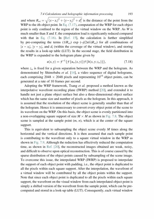
and where Rwi ¼ffiffiffiffiffiffiffiffiffiffiffiffiffiffiffiffiffiffiffiffiffiffiffiffiffiffiffiffiffiffiffiffiffiffiffiffiffiffiffiffiffiffiffiffiffiffiffix − xið Þ2 þ y − yið Þ2 þ d2i

qis the distance of the point from the

WRP to the ith object point. In Eq. (7.17), computation of the WRP for each objectpoint is only confined to the region of the virtual window on the WRP. As W ismuch smaller than X and Y, the computation load is significantly reduced comparedwith that in Eq. (7.16). In [Ref. 15], the calculation is further simplifiedby pre-computing the terms (1/Rwi) exp (−j(2π/λ)Rwi) for all combinations ofjx − xij, jy − yij, and di (within the coverage of the virtual window), and storingthe results in a look-up table (LUT). In the second stage, the field distribution inthe WRP is expanded to the hologram plane given by

uðx, yÞ ¼ F −1 F uw x, yð Þf gF h x, y; zwð Þf gf g, ð7:18Þwhere zw is fixed for a given separation between the WRP and the hologram. Asdemonstrated by Shimobaba et al. [14], a video sequence of digital holograms,each comprising 2048 � 2048 pixels and representing 1014 object points, can begenerated at a rate of 10 frames per second.

Adopting the WRP framework, Tsang et al. proposed a method known as theinterpolative wavefront recording plane (IWRP) method [20], and extended it tohandle not just a plane object surface but also a three-dimensional object surfacewhich has the same size and number of pixels as the hologram. In this approach, itis assumed that the resolution of the object scene is generally smaller than that ofthe hologram. Hence it is unnecessary to convert every object point of the scene toits wavefront on the WRP. On this basis, the object scene is evenly partitioned intoa non-overlapping square support of size M � M as shown in Fig. 7.8. The objectscene is sampled at the sample point (m, n), which is at the center of the squaresupport.

This is equivalent to subsampling the object scene evenly M times along thehorizontal and the vertical directions. It is then assumed that each sample pointis contributing to the wavefront only to a square virtual window in the WRP asshown in Fig. 7.9. Although the reduction has effectively reduced the computationtime, as shown in Ref. [20], the reconstructed images obtained are weak, noisy,and difficult to observe upon optical reconstruction. This is of course caused by thesparse distribution of the object points caused by subsampling of the scene image.To overcome this issue, the interpolated WRP (IWRP) is proposed to interpolatethe support of each object point with padding, i.e., the object point is duplicated toall the pixels within each square support. After the interpolation, the wavefront ofa virtual window will be contributed by all the object points within the support.Note that since each object point is duplicated to all the pixels within each squaresupport, the wavefront on the visual window from each interpolated object point issimply a shifted version of the wavefront from the sample point, which can be pre-computed and stored in a look-up table (LUT). Consequently, each virtual window


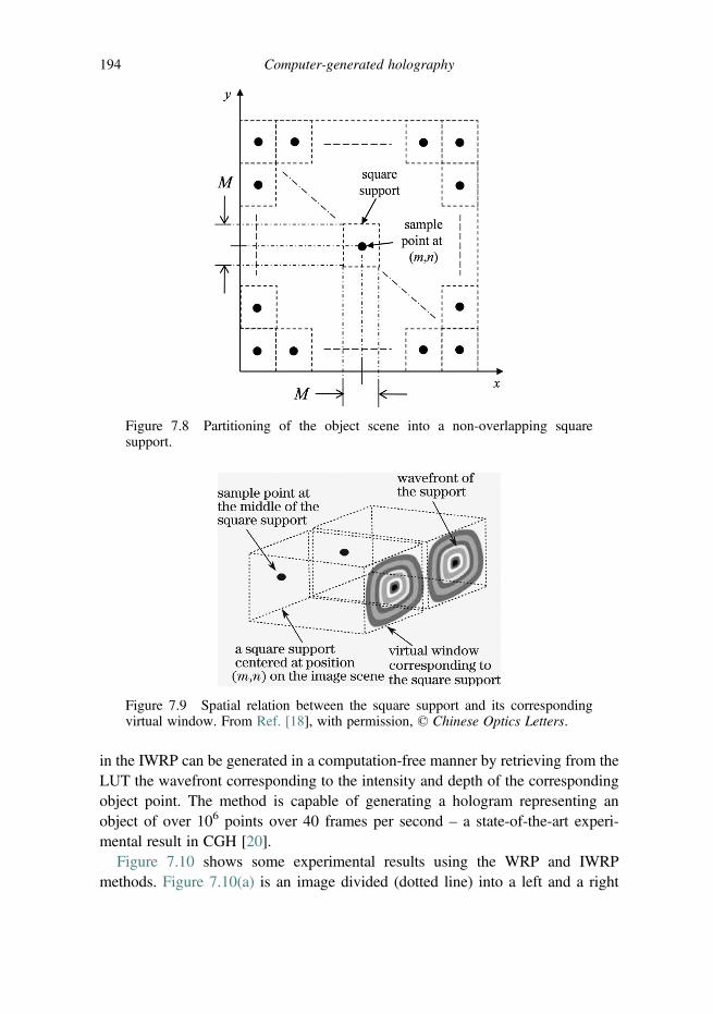
in the IWRP can be generated in a computation-free manner by retrieving from theLUT the wavefront corresponding to the intensity and depth of the correspondingobject point. The method is capable of generating a hologram representing anobject of over 106 points over 40 frames per second – a state-of-the-art experi-mental result in CGH [20].

Figure 7.10 shows some experimental results using the WRP and IWRPmethods. Figure 7.10(a) is an image divided (dotted line) into a left and a right

Figure 7.9 Spatial relation between the square support and its correspondingvirtual window. From Ref. [18], with permission, © Chinese Optics Letters.

Figure 7.8 Partitioning of the object scene into a non-overlapping squaresupport.


part, positioned at distances of z1 ¼ 0.005 m and z2 ¼ 0.01 m from theWRP/IWRP. The image is of 2048 � 2048 square pixels each with a size of9 � 9 μm2 and quantized with 8 bits. Each pixel in the image is taken to generatethe hologram, constituting a total of around 4 � 106 object points. Figure 7.10 (b)to (d) are optically reconstructed real off-axis holograms. The hologram H x, yð Þ isgenerated by multiplying a planar reference wave e−jk0y sin θ (illuminating atan inclined angle θ ¼ 1.2° on the hologram) by u(x, y), and taking the real partof the result given by

H x, yð Þ ¼ Re�u x, yð Þe−jk0y sin θ�, ð7:19Þ

where Re[�] denotes taking the real part of the complex function in brackets. Thehologram is displayed on a liquid crystal on silicon (LCOS) modified from theSony VPL-HW15 Bravia projector. The projector has a horizontal and verticalresolution of 1920 and 1080, respectively. Due to the limited size and resolution ofthe LCOS, only part of the hologram (and hence the reconstructed image) can bedisplayed. Employing the WRP method, the reconstructed images corresponding

Figure 7.10 (a) An image divided (dotted line) into left and right parts, pos-itioned at z1 ¼ 0.005 m (left) and z2 ¼ 0.01 m (right) from the WRP/IWRP,respectively. The WRP/IWRP is positioned at zw ¼ 0.4 m from the hologram; (b)optically reconstructed upper half of the image using the WRP method, (c) sameas (b) but for the lower half of the image, (d) optically reconstructed upper half ofthe image using the IWRP method, and (e) same as (d) but for the lower half ofthe image. From Ref. [20], with permission, © OSA.


to the upper half and the lower half of the hologram are shown in Figs. 7.10(b) and7.10(c), respectively. We observe that the images are extremely weak and noisy.Next we repeat the above process using the IWRP method with M � M ¼ 8 � 8.The reconstructed images are shown in Figs. 7.10(d) and 7.10(e). Evidently, thereconstructed image is much clearer in appearance. To illustrate further the useful-ness of the method, a sequence of holograms of a rotating globe rendered with thetexture of the Earth was generated. The radius of the globe is around 0.005 m, andthe front tip of the globe is located at 0.01 m from the IWRP. The IWRP is at adistance of 0.4 m from the hologram. For a hologram (as well as image size) of2048 � 2048 pixels, the method is capable of attaining a generation speed of over40 frames per second [20].

7.4.2 Holographic information processing

Aside from the rejection of the zeroth-order light and the twin image, in recentyears, the post-processing of digital holographic information, i.e., processing ofrecorded holographic information, has been most studied. Research in this area, forexample sectioning in digital holography, seems to have started in 2006 [21–23]and recent work on optimization using the L2 norm method has led to impressivesectioning results [24], which has motivated the use of the L1 norm, eventuallyleading to what is commonly known as compressive holography [25]. In thissection, we discuss recent innovations in post-processing. Post-processing is basedon the principle of the virtual diffraction plane (VDP) – a generalization of theWRP previously discussed. The principle of VDP-based holographic processinghas three stages as shown in Fig. 7.11.

The conceptual idea of VDP-based holographic processing can be visualizedphysically with the help of Fig. 7.7, where we introduced the concept of the WRP.Now, as shown in Fig. 7.11, we first back-project the hologram to a virtual planecalled the virtual diffraction plane (VDP). In a sense the WRP is now called theVDP. The VDP is close to the original three-dimensional object. Due to the closeproximity, the wave emitted from each object point will only cover a small,localized area on the VDP (in contrast with the wave projected onto the hologram,

Figure 7.11 Hologram post-processing based on the VDP framework.


which covers the entire area). As a result, the overall diffraction pattern on theVDP, which is the summation of the contribution of individual object points, canbe deduced with a very small amount of computation. The rationale is that the VDPis found to carry the diffraction fringes of the entire hologram, but at the same timeit carries similar optical properties as the object scene. Generally speaking, thisimplies that modifying the brightness and contrast on the VDP will lead to almostidentical changes in the pictorial contents it represents. Along this line of thinking,a hologram can revert into a VDP. The information on the VDP can be conveni-ently processed using many existing image processing techniques and tools.Therefore, in the second stage shown in Fig. 7.11, we perform image processingon the VDP. After processing, the VDP can be easily expanded into the ultimatehologram by forward projection, which is further away from the object scene.

Let us now formulate the idea mathematically. Suppose the VDP is located at anaxial distance zv from the hologram, the complex wavefront uVDP(x, y) on the VDPis back-propagated from the hologram t(x, y) given by

uVDP x, yð Þ ¼ t x, yð Þ h x, y; −zvð Þ ¼ t x, yð Þ h x, y; zvð Þ: ð7:20ÞIn the second stage, a selected region(s) on the VDP, denoted by S, is processedwith a given function P[.]. After the modification, the diffraction pattern on theVDP becomes

v x, yð Þ ¼ P uVDP x, yð Þ½ � ðx, yÞ 2 SuVDP x, yð Þ otherwise:

�ð7:21Þ

In the third stage of the VDP processing framework, the modified or the processedwavefront v(x, y) is forward projected onto a hologram plane by convolving withthe spatial impulse response in Fourier optics given by

tP x, yð Þ ¼ v x, yð Þ h x, y; zvð Þ: ð7:22ÞWe can realize Fourier transformation in Eqs. (7.20) and (7.22), and the Fouriertransform of h(x, y; zv) and h

*(x, y; zv) can be pre-computed in advance. Hence, theprocessing of a hologram with the VDP framework mainly involves a pair offorward and inverse Fourier transform operations. The rest of the process isnegligible with regard to computation time. Based on a commercial graphicprocessing unit (GPU) to conduct the Fourier transform, a medium size digitalhologram comprising 2048 � 2048 pixels can be processed in less than 10 ms,equivalent to a rate of over 100 frames per second [26].

Figure 7.12 shows an example of VDP-based processing of the hologram. Apartfrom readjusting the brightness and contrast of the image represented in a holo-gram, sometimes it is also necessary to enhance the sharpness in certain regions toincrease the visibility of the high frequency contents. This process can be achieved


by applying a high-boost filter to the selected area on the VDP of the hologram.High-boost filtering is performed by amplifying the original input image and thensubtracting a lowpass image, which is given by

v x,yð Þjðx,yÞ2S ¼hAuVDP x, yð Þ−BuLVDPðx, yÞ

i, ð7:23Þ

where uLVDPðx, yÞ is a lowpass version of the region S. Each pixel in uLVDPðx, yÞ isderived from the average value of a 3 � 3 window centered at the correspondingpixel according to

uLVDP x, yð Þ ¼ 19

X1m¼−1

X1n¼−1

uVDP xþ m, yþ nð Þ: ð7:24Þ

The terms A and B are constant values. The larger the values of A and B, the higherwill be the brightness and sharpness of the region S, respectively. Other types ofsharpening filters can be applied under the same principle. The hologramsharpening process is illustrated by a hemisphere with the texture of the Earth asshown in Fig. 7.12. The hemisphere has a radius of 5 mm with its tip located at0.3 m from the hologram. Once the digital hologram is obtained, the VDP isgenerated using Eq. (7.20). The high-boost filter in Eq. (7.23) is applied to theVDP, and subsequently forward projected into a hologram using Eq. (7.22). Thereconstructed image of the modified hologram, focused at 0.3 m (which causesslight de-focusing around the rim of the hemisphere), is shown in Fig. 7.12(b). Itcan be seen that the edge on the left side of the reconstructed image isstrengthened, and the rest of the reconstructed image is not affected as S, theregion to be processed, has been chosen to the right half of the plane.

Figure 7.12 (a) A hemisphere rendered with the texture of the Earth positionedat 0.3 m from the hologram plane. (b) Numerical reconstructed image of thehologram representing the image in (a) after direct application of high-boostfiltering to the left side of the virtual diffraction plane. From Ref. [26], withpermission, © OSA.


7.5 Three-dimensional holographic display using spatial light modulators

Static holograms with high fidelity have been achievable for a long time, but thereal-time display of high-quality digital holograms remains a challenge due to thelimitations of modern SLMs. The real-time display of digital holograms demandsspatial light modulators (SLMs) of high resolution and with the capability ofupdating frames at video rate [27]. In this section, we consider some of the issuesin real-time holographic display. Of course, other practical issues such as phaseuniformity over the SLM surface (which is important as high-quality read-outemploys coherent light) and large-area format would also need to be taken intoaccount for any practical real-time display system.

7.5.1 Resolution

To consider the high resolution issue, for simplicity, let us display an on-axis pointsource hologram as an example. According to Chapter 2, the on-axis point sourcehologram is given by

t x, yð Þ ¼ Aþ B sink02z0

x2 þ y2� �

: ð7:25Þ

Again, z0 is the distance of the point source from the hologram. An instantaneousspatial frequency along the x-direction within the hologram is

f inst xð Þ ¼ 12π

d

dx

k02z0

x2 �

¼ x

λz0: ð7:26Þ

Assuming the SLM is limited to the size xmax with spatial resolution f0, then thehighest spatial frequency of the hologram fringes is finst (xmax) ¼ xmax/λz0 and if wewant to record it, we must set

f inst xmaxð Þ ¼ xmaxλz0

¼ f 0: ð7:27Þ

Hence, for a given spatial resolution of the SLM, we can find the limiting aperture,xmax, of the hologram on the SLM. We define the numerical aperture of thehologram as

NA ¼ sinθ2

� �¼ xmaxffiffiffiffiffiffiffiffiffiffiffiffiffiffiffiffiffiffi

x2max þ z20p ¼ xmax

z01þ xmax

z0

� �2" #−0:5

, ð7:28Þ

where θ is the viewing angle as shown in Fig. 7.13, as the on-axis hologram isreconstructed with a real point source located z0 away from the hologram.

7.5 Display using spatial light modulators 199

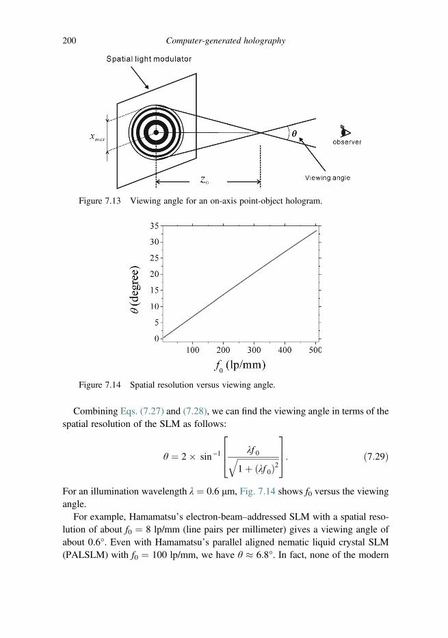
Combining Eqs. (7.27) and (7.28), we can find the viewing angle in terms of thespatial resolution of the SLM as follows:

θ ¼ 2� sin −1 λf 0ffiffiffiffiffiffiffiffiffiffiffiffiffiffiffiffiffiffiffiffi1þ λf 0ð Þ2

q264

375: ð7:29Þ

For an illumination wavelength λ ¼ 0.6 μm, Fig. 7.14 shows f0 versus the viewingangle.

For example, Hamamatsu’s electron-beam–addressed SLM with a spatial reso-lution of about f0 ¼ 8 lp/mm (line pairs per millimeter) gives a viewing angle ofabout 0.6°. Even with Hamamatsu’s parallel aligned nematic liquid crystal SLM(PALSLM) with f0 ¼ 100 lp/mm, we have θ � 6.8°. In fact, none of the modern

Figure 7.14 Spatial resolution versus viewing angle.

Figure 7.13 Viewing angle for an on-axis point-object hologram.


SLMs, typically with a spatial resolution of about 100 lp/mm, are suitable for largeviewing angle three-dimensional display. Since 1 lp/mm means there are twopixels in 1 mm, 100 lp/mm means the pixel size is about 1

2 � 1100 mm or 5 μm for

modern SLMs. The situation becomes even worse if off-axis holography isemployed because the SLM needs to resolve the carrier frequency. For an offsetangle of 45°, the spatial carrier frequency is sin 45°/λ � 1000 lp/mm or a pixel sizeof about 0.5 μm, well beyond modern SLM capability. Hence high resolutionholographic display with SLMs is an important area of research.

An effective solution for higher resolution holographic display has beenrealized through the integration of optically addressed SLMs and the active tiltingmethod [28, 29]. But both the cost and complexity of such systems are high.Here we discuss a modern approach to address the issue of low resolutionSLMs. The type of novel digital hologram generated is called a binary maskprogrammable hologram (BMPH) [30].

7.5.2 Digital mask programmable hologram

In contrast to the classical digital Fresnel hologram, a BMPH comprises a static,high resolution binary grating, G(x, y), which is overlaid with a lower resolutionbinary mask,M(x, y). The reconstructed image of the BMPH can be programmed toapproximate a target image (including both intensity and depth information) byconfiguring the pattern of the binary mask with a simple genetic algorithm (SGA).As the low resolution binary mask can be realized using less stringent displaytechnology, the method allows the development of simple and economical holo-graphic video display. Figure 7.15 shows the structure of the BMPH. The patternG(x, y) is a static, high resolution binary diffraction grating where each pixel iseither transparent or opaque. A checkerboard pattern is used for G(x, y) so thatthe frequency of the grating pattern is maximum along both the horizontal andvertical directions to provide uniform diffraction efficiency along the two directions.The pattern M(x, y) is a binary mask pattern that is lower in resolution than thegrating, and is evenly partitioned into square blocks each with a size k � k pixels,where k is an integer that is larger than unity. Within each square block, all thepixels are identical and set to be either transparent or opaque. As such, the resolutionof the mask pattern is (1/k)th of that of G(x, y) along the horizontal and verticaldirections. Superposition of the pair of images results in the BMPH given by

B x, yð Þ ¼ Gðx, yÞMðx, yÞ: ð7:30ÞFor a given B(x, y) as a hologram, we can determine the location where the

image is reconstructed using the diffraction theory developed in Chapter 2. Withreference to Eq. (1.30), for a given spectrum of the field distribution Ψp0 kx, ky

� ,


which is the Fourier transform of the field ψp0 x, yð Þ at z ¼ 0, we write the complexfield at z given by

ψp x, y; zð Þ ¼ F −1 Ψp0 kx, ky�

exp −jk0zzð Þ� �with k0z ¼ k0

ffiffiffiffiffiffiffiffiffiffiffiffiffiffiffiffiffiffiffiffiffiffiffiffiffiffiffiffiffiffiffiffiffiffiffiffiffiffiffi1 − k2x=k

20 − k

2y=k

20

� �rfor waves propagating in the positive

z-direction. By substituting Ψp0 kx, ky� ¼ F ψp0 x, yð Þ

n ointo the above equation,

we can express ψp(x, y;z) as

ψp x, y; zð Þ ¼ ψp0 x, yð Þ hr x, y; zð Þ ¼ðð∞−∞

ψp0 x0, y0ð Þhr x − x0, y − y0; zð Þdx0dy0, ð7:31Þ

where

hr x, y; zð Þ ¼ F −1 exp −jk0

ffiffiffiffiffiffiffiffiffiffiffiffiffiffiffiffiffiffiffiffiffiffiffiffiffiffiffiffiffiffiffiffiffiffiffiffiffiffiffi1 − k2x=k

20 − k

2y=k

20

� �rz

�� :

hr(x, y;z) is called the spatial impulse response of propagation of light [31]. Theexact inverse transform has been given but is fairly complicated. For z that is manywavelengths away from ψp0(x, y) and with the paraxial approximation in the spatialdomain, i.e., x2 þ y2 � z2, for any amplitude factors, hr(x, y;z) becomes

hr x, y; zð Þ ¼jk0 exp −jk0

ffiffiffiffiffiffiffiffiffiffiffiffiffiffiffiffiffiffiffiffiffiffiffiffix2 þ y2 þ z2

ph i2πz

: ð7:32Þ

Figure 7.15 Structure of the binary mask programmable hologram, a lowresolution binary mask overlaid onto a high resolution binary grating.From Ref. [30], with permission, © OSA.


If we go further using the paraxial approximation in the phase factor aboveas well, we recover h(x, y;z), the spatial impulse response in Fourier optics[see Eq. (1.34), or [31]]. Now, incoporating Eq. (7.31) into Eq. (7.32),we have

ψp x, y; zð Þ ¼ jk02πz

ðð∞−∞

ψp0 x0, y0ð Þexp −jk0

ffiffiffiffiffiffiffiffiffiffiffiffiffiffiffiffiffiffiffiffiffiffiffiffiffiffiffiffiffiffiffiffiffiffiffiffiffiffiffiffiffiffiffiffiffiffiffiðx − x0Þ2 þ ðy − y0 Þ2 þ z2

q �dx0dy0, ð7:33Þ

which becomes the Fresnel diffraction formula in Eq. (1.35) when x2 þ y2 � z2 isused in the phase term for the approximation. We shall use Eq. (7.33) to formulatethe solution for the BMPH.

When the BMPH hologram, B(x, y), is illuminated with an on-axis planarcoherent beam, the magnitude of the reconstructed image at distance zd can beexpressed as

Id x, yð Þ ¼XX − 1

p¼ 0

XY − 1

q¼ 0

Bðp, qÞexp −jk0

ffiffiffiffiffiffiffiffiffiffiffiffiffiffiffiffiffiffiffiffiffiffiffiffiffiffiffiffiffiffiffiffiffiffiffiffiffiffiffiffiffiffiffiffiffiffiffiffiffiffiffiffiffiffiffiffiffiffiffiffiðx − pÞδd½ �2 þ ðy − qÞδd½ �2 þ z2d

q �, ð7:34Þ

where X � δd and Y � δd are the horizontal and vertical extents of the hologram,respectively, as δd is the width and the height of a pixel in B(x, y). Note that theabove equation in double summations is simply a discrete version of Eq. (7.33),where we have neglected any constants in front of the integration. Without loss ofgenerality, we assume that the hologram and the image scene have identicalhorizontal and vertical extents. From Eqs. (7.30) and (7.34), we can deduce thatthe reconstructed image is dependent on the binary mask pattern, M(x, y). How-ever, given Id(x, y) there is no explicit inverse formulation to compute M(x, y).In view of this, the inverse problem has been treated as an optimization process todetermine the mask pattern that best approximates the target reconstructed image.To begin with, an objective function Od is defined to determine the root-mean-square error (RMSE) [see Eq. (7.15)] between the reconstructed image Id(x, y) anda planar target image Td(x, y) which is located at a distance zd from the hologramsuch that

Od ¼ffiffiffiffiffiffiffiffiffiffiffiffiffiffiffiffiffiffiffiffiffiffiffiffiffiffiffiffiffiffiffiffiffiffiffiffiffiffiffiffiffiffiffiffiffiffiffiffiffiffiffiffiffiffiffiffiffiffiffiffiffi1XY

XX − 1

p¼ 0

XY−1q¼ 0

Td p,qð Þ− Idðp,qÞ½ �2vuut : ð7:35Þ

The goal is to determine M(x, y) so that the value of Od is minimized. It isimportant to point out that this is different from determining a binary hologramB(x, y) that matches the binary hologram of a given target image Td(x, y). If this is


the case, the resolution of B(x, y) will have to be identical to that of the highresolution grating. In this method, a low resolution mask M(x, y) is determinedso that when it is coupled with the grating, it will result in a reconstructed imagethat is similar to the target. This is a formidable problem that cannot be solved withbrute-force means (such as blind search), as there are 2XY=k

2combinations on the

mask pattern that can be represented in M(x, y). For example, for a modest squarehologram with X and Y both equal to 256, and k ¼ 4, the total number of patternsthat can be generated is 24096. In view of this, a simple genetic algorithm (SGA)has been employed [32], a method that mimics the evolutionary mechanism inbiological species, to determine the optimal mask pattern. Past research hasdemonstrated that the SGA is effective in solving complicated optimization prob-lems in many engineering applications [33]. As the principles and details of theSGA have been described in the literature, we shall only present results here.The effect of the use of a low resolution SLM for holographic display is shown inFig. 7.16. Obviously, the low resolution SLM with 20 μm pixel size has problemsreconstructing the hologram as shown in Fig. 7.16(c), whereas the SLM with 5 μmpixel size can display the hologram reasonably well.

When the BMPH is generated for the target image shown in Fig. 7.16(a) withgrating size 256 � 256 pixels and pixel size 5 μm square, and a binary mask of64 � 64 pixels (shown in Fig. 7.17(a)) with pixel size 20 μm, which is four timesworse than that of the Fresnel hologram as k ¼ 4, the reconstructed image is asshown in Fig. 7.17(b).

The main feature of a MPBH is that the target image it represents canbe composed by simply changing the pattern on the binary mask. As the binarymask can be implemented with less stringent electronic devices, the method canbe used for holographic display where high resolution SLMs are simply notavailable.

Figure 7.16 (a) A planar image placed at 0.4 m from the hologram. (b) Simulatedreconstructed image of the hologram display by a SLM of pixel size 5 μm at0.4 m. (c) Same as (b) but with SLM of pixel size 20 μm. The number ofhologram samples is 256 � 256 and the wavelength of light used is 0.65 μm.From Ref. [30], with permission, © OSA.


7.5.3 Real-time display

For a given spatial resolution of a SLM, f0, and according to the Nyquist samplingtheorem, the sampling interval of the displayed hologram is Δx¼ 1/2f0. In terms ofthe NA, we have Δx ¼ λ/2NA. Assuming the size of the SLM is L � L, the numberof samples or resolvable pixels for full parallax is therefore

NFull−p ¼ L

Δx

� �2

¼ L� 2NAλ

� �2

: ð7:36Þ

For a full parallax L� L¼ 30 mm� 30 mm on-axis hologram presented on a SLM,and a viewing angle of θ ¼ 60°, the required number of resolvable pixels is about2.25� 109 for λ¼ 0.6328 μm. So we are talking about a 2.25 gigapixel SLM and, toput things into perspective, some of the best modern CCD cameras are about 22megapixels, that is about two orders ofmagnitude difference between the two devicesin terms of the required numbers of pixels. Indeed the required number of resolvablepixels is well beyond the current capabilities of SLMs.Now ifwewant to update sucha SLM with 8-bit resolution at 30 frames per second, a serial data rate of 2.25 gigasamples/frame � 8 bits/sample � 30 frames/second ¼ 0.54 terabits/second isrequired and even with state-of-the-art 40 gigabit Ethernet connectivity, it falls shortof what we need for the transfer rate. Holographic information reduction has thusbecome one of the most important topics in real-time holographic display research.

Horizontal parallax-only (HPO) holography is an excellent way to reduce holo-graphic information [34, 35]. The basic idea is that since we are used to looking at theworld with our two eyes more or less on a horizontal level, we are usually satisfiedwith only horizontal parallax. Hence for 256 vertical lines, the number of pixelsrequired is

NHPO ¼ 256� L

Δx

� �� 12:1 million, ð7:37Þ

Figure 7.17 (a) Binary mask corresponding to the target image in Fig. 7.16(a).(b) Reconstructed image of the BMPH at 0.4 m. From Ref. [30], with permission,© OSA.


compared to the case of full parallax of 2.4 gigapixels. The serial data rate reduces to12.1 million samples/frame � 8 bits/sample � 30 frames/second ¼ 2.9 gigabits/second, which is quite manageable with a modern Ethernet connection. HenceHPO holography aims to record and reconstruct HPO information andmany HPO holographic systems have been proposed and studied [34, 35].The first computer-generated HPO digital holographic system was proposed andconstructed by St. Hilaire et al. [36]. The authors achieved a displayedimage of 5 cm � 3 cm � 3 cm with a viewing angle of about 15°. However, thefirst digital holographic recording technique to be investigated regarding the HPOapproach was that proposed by Poon et al. [37]. The HPO digital holographic systemis based on the principle of optical scanning holography. The idea is fairly simple.Instead of scanning a three-dimensional object with a full two-dimensionaltime-dependent Fresnel zone plate [see Eq. (5.46)] to obtain holographic information,a one-dimensional time-dependent Fresnel zone plate is used to generate HPOholograms. However, these slit-type holograms for each point of the object producevertical spreading and require the use of a cylindrical lens to compensate for thisspreading during reconstruction. Recently, a computer algorithm has been proposedto convert a full parallax hologram to an off-axis HPO hologram for three-dimensional display [38], and three-dimensional display has been achieved [39].However, the display is confined to simple point objects.

7.5.4 Lack of SLMs capable of displaying a complex function

The reconstruction of the complex hologram is free of the zeroth-order light and thetwin image [40]. Unfortunately, modern SLMs can modulate either the phase or theamplitude of incident light, but not both [41, 42]. A brute-force method is to use twoSLMs to display a complex hologram by cascading the SLMs, one for amplitudemodulation and the other for phase modulation [43–45]. Alternatively, a beamsplitter can be used to combine the beams from two SLMs [see Eq. (5.52)], one fordisplaying the real part and the other the imaginary part of the complex hologram[46–48]. Recently, a method has been proposed to display a complex hologram usinga single intensity-modulated hologram [10]. The method involves a standard coher-ent image processing systemwith a grating at the Fourier plane. Two position-shiftedamplitude holograms displayed on a single SLM can be coupled via the grating andautomatically overlapped at the output plane of the image processing system tosynthesize a complex hologram. The processing system is shown in Fig. 7.18.

The two position-shifted holograms, Hr(x − d, y0) and Hi(yþ d, y0) separated bya distance 2d, are displayed on the x0−y0 plane, where Hr(x, y) and Hi(x, y) arethe real part and imaginary part of a complex hologram Hc(x, y) ¼ jHcje jϑ,respectively, given by


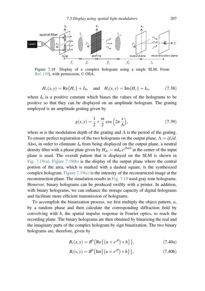
Hrðx, yÞ ¼ Re Hcf g þ I0, and Hiðx, yÞ ¼ Im Hcf g þ I0, ð7:38Þwhere I0 is a positive constant which biases the values of the holograms to bepositive so that they can be displayed on an amplitude hologram. The gratingemployed is an amplitude grating given by

g x, yð Þ ¼ 12þ m

2cos 2π

x

Λ

� �, ð7:39Þ

where m is the modulation depth of the grating and Λ is the period of the grating.To ensure perfect registration of the two holograms on the output plane, Λ ¼ λf1/d.Also, in order to eliminate I0 from being displayed on the output plane, a neutraldensity filter with a phase plate given by Hdc ¼ mI0 e

j5π/4 at the center of the inputplane is used. The overall pattern that is displayed on the SLM is shown inFig. 7.19(a). Figure 7.19(b) is the display of the output plane where the centralportion of the area, which is marked with a dashed square, is the synthesizedcomplex hologram. Figure 7.19(c) is the intensity of the reconstructed image at thereconstruction plane. The simulation results in Fig. 7.19 used gray tone holograms.However, binary holograms can be produced swiftly with a printer. In addition,with binary holograms, we can enhance the storage capacity of digital hologramsand facilitate more efficient transmission of holograms.

To accomplish the binarization process, we first multiply the object pattern, u,by a random phase and then calculate the corresponding diffraction field byconvolving with h, the spatial impulse response in Fourier optics, to reach therecording plane. The binary holograms are then obtained by binarizing the real andthe imaginary parts of the complex hologram by sign binarization. The two binaryholograms are, therefore, given by

Brðx, yÞ ¼ B0 Re u� e jθ� h� ��

, ð7:40aÞBiðx, yÞ ¼ B0 Im u� e jθ

� h� �� , ð7:40bÞ

Figure 7.18 Display of a complex hologram using a single SLM. FromRef. [10], with permission, © OSA.


Figure 7.19 (a) Designed input pattern at the SLM, (b) optical field at the outputplane, and (c) intensity of the reconstructed image at the reconstruction plane.From Ref. [10], with permission, © OSA.

Figure 7.20 (a) Binary hologram Br(x, y), (b) binary hologram Bi(x, y), (c) imagereconstruction using Br(x, y), and (d) image reconstruction using the complexhologram, Br(x, y) þ jBi(x, y). From Ref. [10], with permission, © OSA.See Table 7.4 for the MATLAB code.


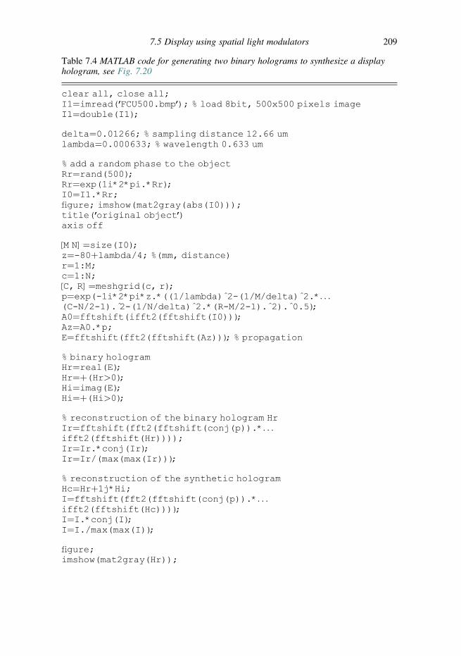
Table 7.4 MATLAB code for generating two binary holograms to synthesize a displayhologram, see Fig. 7.20

clear all, close all;I1¼imread(’FCU500.bmp’); % load 8bit, 500x500 pixels imageI1¼double(I1);

delta¼0.01266; % sampling distance 12.66 umlambda¼0.000633; % wavelength 0.633 um

% add a random phase to the objectRr¼rand(500);Rr¼exp(1i*2*pi.*Rr);I0¼I1.*Rr;figure; imshow(mat2gray(abs(I0)));title(’original object’)axis off

[M N]¼size(I0);z¼-80þlambda/4; %(mm, distance)r¼1:M;c¼1:N;[C, R]¼meshgrid(c, r);p¼exp(-1i*2*pi*z.*((1/lambda) 2̂-(1/M/delta) 2̂.*. . .(C-N/2-1). 2̂-(1/N/delta) 2̂.*(R-M/2-1). 2̂). 0̂.5);A0¼fftshift(ifft2(fftshift(I0)));Az¼A0.*p;E¼fftshift(fft2(fftshift(Az))); % propagation

% binary hologramHr¼real(E);Hr¼þ(Hr>0);Hi¼imag(E);Hi¼þ(Hi>0);

% reconstruction of the binary hologram HrIr¼fftshift(fft2(fftshift(conj(p)).*. . .ifft2(fftshift(Hr))));Ir¼Ir.*conj(Ir);Ir¼Ir/(max(max(Ir)));

% reconstruction of the synthetic hologramHc¼Hrþ1j*Hi;I¼fftshift(fft2(fftshift(conj(p)).*. . .ifft2(fftshift(Hc))));I¼I.*conj(I);I¼I./max(max(I));

figure;imshow(mat2gray(Hr));


where θ is a random phase function between 0 and 2π and B0{.} is the binarizationoperator with the threshold value set to zero, i.e., if the input value is larger thanzero, then the output value is 1, otherwise the output value is zero. The purpose ofthe random phase is to reduce the edge effect caused by binarization.

The two binary holograms Br(x, y) and Bi(x, y) for the text “FCU” are shown inFigs. 7.20(a) and (b), respectively. Figure 7.20(c) is the reconstruction of a singlebinary hologram, while Fig. 7.20(d) shows the reconstruction of the synthesizedcomplex hologram. The MATLAB code is listed in Table 7.4. Although someartifacts due to the binarization process exist, most of the background noise,such as the noise due to the twin image, has been removed, as shown inFig. 7.20(d). For optical reconstruction of Br(x, y) and Bi(x, y) using the systemshown in Fig 7.18, readers are encouraged to check Ref. [10].

Problems

7.1 Generate a detour-phase CGH in MATLAB by setting ℓ ¼ 1 in Eq. (7.12).Note that there may now be crosstalk between adjacent cells.

7.2 In developing the detour-phase CGH, we have applied some approximations,and they are

pmnk0dx2πf

� 1,qmnk0dy2πf

� 1, f sin θ � dxpmn sin θ � λ,

andk0fαmndx � 1:

Table 7.4 (cont.)

title(’Binary hologram B_r’)axis off

figure;imshow(mat2gray(Hi));title(’Binary hologram B_i’)axis off

figure;imshow(3*Ir);title(’reconstructed image of B_r’)axis off

figure;imshow(3*I);title(’Reconstructed image of the syntheti chologram’)axis off


Propose a design strategy (i.e., determine the hologram size, cell size, windowsize. . .) so that all the approximations can be satisfied.

7.3 Equation (7.26) is a formula derived under the paraxial approximation. Derivethe local fringe frequency of the interferogram formed by a plane wave and aspherical wave without applying the paraxial approximation. Then go on toshow that the viewing angle becomes

θ ¼ 2� sin −1 λf 0½ �instead of the angle derived under the paraxial approximation given byEq. (7.29). Finally plot θ versus f0 for f0 up to 1000 lp/mm at λ ¼ 0.6 μm.

References

1. B. R. Brown, and A. W. Lohmann, Complex spatial filtering with binary masks,Applied Optics 5, 967–969 (1966).

2. A. W. Lohmann, and D. P. Paris, Binary Fraunhofer holograms, generated by com-puter, Applied Optics 6, 1739–1748 (1967).

3. L. B. Lesem, P. M. Hirsch, and J. A. Jordan, The kinoform: a new wavefrontreconstruction device, IBM Journal of Research and Development 13, 150–155(1969).

4. N. C. Gallagher, and B. Liu, Method for computing kinoforms that reduces imagereconstruction error, Applied Optics 12, 2328–2335 (1973).

5. B. Liu, and N. C. Gallagher, Convergence of a spectrum shaping algorithm, AppliedOptics 13, 2470–2471 (1974).

6. P. M. Hirsch, J. J. A. Jordan, and L. B. Lesem, Method of making an object-dependentdiffuser, U.S. patent 3,619,022 (1971).

7. R. W. Gerchberg, and W. O. Saxton, A practical algorithm for the determination ofphase from image and diffraction plane pictures, Optik 35, 237–246 (1972).

8. J. R. Fienup, Phase retrieval algorithms: a comparison, Applied Optics 21, 2758–2769(1982).

9. J. R. Fienup, Phase retrieval algorithms: a personal tour [Invited], Applied Optics 52,45–56 (2013).

10. J.-P. Liu, W.-Y. Hsieh, T.-C. Poon, and P. Tsang, Complex Fresnel hologram displayusing a single SLM, Applied Optics 50, H128–H135 (2011).

11. L. C. Ferri, Visualization of 3D information with digital holography using laserprinters, Computer & Graphics 25, 309–321 (2001).

12. H. Yoshikawa, and M. Tachinami, Development of direct fringe printer for computer-generated holograms, Proceedings SPIE 5742, 259–266 (2005).

13. T. Shimobaba, N. Masuda, and T. Ito, Simple and fast calculation algorithm forcomputer-generated hologram with wavefront recording plane, Optics Letters 34,3133–3135 (2009).

14. T. Shimobaba, H. Nakayama, N. Masuda, and T. Ito, Rapid calculation algorithm ofFresnel computer-generated-hologram using look-up table and wavefront-recordingplane methods for three-dimensional display, Optics Express 18, 19504–19509(2010).

15. T. Yamaguchi, G. Okabe, and H. Yoshikawa, Real-time image plane full-color andfull-parallax holographic video display system, Optical Engineering 46, 125801(2007).

References 211

16. P. Tsang, J.-P. Liu, W.-K. Cheung, and T.-C. Poon, Fast generation of Fresnelholograms based on multirate filtering, Applied Optics 48, H23–H30 (2009).

17. S.-C. Kim, J.-H. Kim, and E.-S. Kim, Effective reduction of the novel look-uptable memory size based on a relationship between the pixel pitch and reconstruc-tion distance of a computer-generated hologram, Applied Optics 50, 3375–3382(2011).

18. P. W. M. Tsang, and T. C. Poon, Review on theory and applications of wavefrontrecording plane framework in generation and processing of digital holograms, ChineseOptics Letters 11, 010902 (2013).

19. T.-C. Poon, On the fundamentals of optical scanning holography, American Journal ofPhysics 76, 739–745 (2008).

20. P. Tsang, W. K. Cheung, T. C. Poon, and C. Zhou, Holographic video at 40 framesper second for 4-million object points, Optics Express 19, 15205–15211 (2011).

21. A. Anand, and S. Vijay Raj, Sectioning of amplitude images in digital holography,Measurement Science and Technology 17, 75–78 (2006).

22. W.-C. Chien, D. S. Dilworth, E. Liu, and E. N. Leith, Synthetic-aperture chirpconfocal imaging, Applied Optics 45, 501–510 (2006).

23. T. Kim, Optical sectioning by optical scanning holography and a Wiener filter,Applied Optics 45, 872–879 (2006).

24. X. Zhang, E. Y. Lam, and T.-C. Poon, Reconstruction of sectional images in holog-raphy using inverse imaging, Optics Express 16, 17215–17226 (2008).

25. D. J. Brady, K. Choi, D. L. Marks, R. Horisaki, and S. Lim, Compressive holography,Optics Express 17, 13040–13049 (2009).

26. P. W. M. Tsang, T. C. Poon, and K. W. K. Cheung, Enhancing the pictorial content ofdigital holograms at 100 frames per second, Optics Express 20, 14183–14188 (2012).

27. T.-C. Poon, Three-dimensional television using optical scanning holography, Journalof Information Display 3, 12–16 (2002).

28. M. Stanley, R. W. Bannister, C. D. Cameron, S. D. Coomber, I. G. Cresswell, J. R.Hughes, V. Hui, P. O. Jackson, K. A. Milham, R. J. Miller, D. A. Payne, J. Quarrel,D. C. Scattergood, A. P. Smith, M. A. G. Smith, D. L. Tipton, P. J. Watson, P. J.Webber, and C. W. Slinger, 100-megapixel computer-generated holographic imagesfrom active tiling: a dynamic and scalable electro-optic modulator system, Proceed-ings SPIE 5005, 247–258 (2003).

29. H.-S. Lee, H. Song, S. Lee, N. Collings, and D. Chu, High resolution spatial lightmodulator for wide viewing angle holographic 3D display, in Collaborative Confer-ence on 3D Research (CC3DR), (2012), pp. 71–72.

30. P. W. M. Tsang, T. C. Poon, C. Zhou, and K. W. K. Cheung, Binary mask program-mable hologram, Optics Express 20, 26480–26485 (2012).

31. T.-C. Poon, and T. Kim, Engineering Optics with MATLAB (World Scientific,Singapore, 2006).

32. D. Goldberg, Genetic Algorithms in Search, Optimization, and Machine Learning(Addison-Wesley, Boston, MA, 1989).

33. A. M. Zalzala, and P. J. Fleming, eds., Genetic Algorithms in Engineering Systems(Institution of Electrical Engineers, Stevenage, UK, 1997).

34. S. A. Benton, The mathematical optics of white light transmission holograms, inInternational Symposium on Display Holography (Lake Forest College, Lake Forest,July 1982).

35. C. P. Grover, R. A. Lessard, and R. Tremblay, Lensless one-step rainbow holographyusing a synthesized masking slit, Applied Optics 22, 3300–3304 (1983).


36. P. St. Hilaire, S. A. Benton, and M. Lucente, Synthetic aperture holography: a novelapproach to three-dimensional displays, Journal of the Optical Society of America A 9,1969–1977 (1992).

37. T.-C. Poon, T. Akin, G. Indebetouw, and T. Kim, Horizontal-parallax-only electronicholography, Optics Express 13, 2427–2432 (2005).

38. T. Kim, Y. S. Kim, W. S. Kim, and T.-C. Poon, Algorithm for converting full-parallaxholograms to horizontal-parallax-only holograms, Optics Letters 34, 1231–1233(2009).

39. Y. S. Kim, T. Kim, T.-C. Poon, and J. T. Kim, Three-dimensional display of ahorizontal-parallax-only hologram, Applied Optics 50, B81–B87 (2011).

40. T.-C. Poon, T. Kim, G. Indebetouw, B. W. Schilling, M. H. Wu, K. Shinoda, andY. Suzuki, Twin-image elimination experiments for three-dimensional images inoptical scanning holography, Optics Letters 25, 215–217 (2000).

41. B. E. A. Saleh, and K. Lu, Theory and design of the liquid crystal TV as an opticalspatial phase modulator, Optical Engineering 29, 240–246 (1990).

42. J. A. Coy, M. Zaldarriaga, D. F. Grosz, and O. E. Martinez, Characterization of aliquid crystal television as a programmable spatial light modulator, Optical Engineer-ing 35, 15–19 (1996).

43. L. G. Neto, D. Roberge, and Y. Sheng, Full-range, continuous, complex modulationby the use of two coupled-mode liquid-crystal televisions, Applied Optics 35, 4567–4576 (1996).

44. R. Tudela, I. Labastida, E. Martin-Badosa, S. Vallmitjana, I. Juvells, and A. Carnicer,A simple method for displaying Fresnel holograms on liquid crystal panels, OpticsCommunications 214, 107–114 (2002).

45. M.-L. Hsieh, M.-L. Chen, and C.-J. Cheng, Improvement of the complex modulatedcharacteristic of cascaded liquid crystal spatial light modulators by using a novelamplitude compensated technique, Optical Engineering 46, 070501 (2007).

46. R. Tudela, E. Martín-Badosa, I. Labastida, S. Vallmitjana, I. Juvells, and A. Carnicer,Full complex Fresnel holograms displayed on liquid crystal devices, Journal of OpticsA: Pure and Applied Optics 5, S189 (2003).

47. R. Tudela, E. Martín-Badosa, I. Labastida, S. Vallmitjana, and A. Carnicer, Wavefrontreconstruction by adding modulation capabilities of two liquid crystal devices, OpticalEngineering 43, 2650–2657 (2004).

48. S.-G. Kim, B. Lee, and E.-S. Kim, Removal of bias and the conjugate image inincoherent on-axis triangular holography and real-time reconstruction of the complexhologram, Applied Optics 36, 4784–4791 (1997).

References 213

Index

aliasing 83 (see also spectral folding)amplitude 27amplitude transmittance 5 (see also transparency

function)angular plane wave spectrum 8angular spectrum method (ASM) 95

(see also convolution method, double Fouriertransform method)

bipolar point spread function 21

charge-coupled device (CCD) 89–90chromatic aberration 40–2coherence length 46, 50transverse 53

coherence time 46, 50coherent image processing 17coherent optical system 17coherent point spread function (CPSF) 16coherent transfer function (CTF) 16complementary metal-oxide- semiconductor (CMOS)

89–90complex amplitude 5, 27complex degree of coherence 43complex degree of mutual coherence 52complex degree of self coherence 52conjugate beam 73contour 169contouringtwo-wavelength 169–70two-illumination 172–4

convolution integral 10convolution method 95 (see also angular spectrum

method, double Fourier transform method)

double Fourier transform method 95 (see also angularspectrum method, convolution method)

equivalent wavelength 169 (see also syntheticwavelength)

Ewald equation 136Ewald sphere 136

fill factor 90first Born approximation 134first Rytov approximation 134four-f system 15Fourier plane 15Fourier transform

discrete (DFT) 82, 95fast 83inverse 6inverse discrete (IDFT) 82, 95inverse temporal 47one-dimensional temporal 47spectroscopy 49three-dimensional 135two-dimensional 6

Fraunhofer approximation 12Fraunhofer diffraction formula 12frequency resolution 81Fresnel diffraction formula 10, 203Fresnel diffraction method (FDM) 99Fresnel zone plate (FZP) 30, 91

time-dependent (TDFZP) 140fringe visibility 44 (see also visibility)

Gerchberg–Saxton algorithm 187 (see also iterativeFourier transform algorithm)

graphic processing unit (GPU) 197Green’s function 134

height sensitivity 169Helmholtz equation 5, 133hologram 28

binary mask programmable (BMPH) 201carrier frequency 62 (see also hologram, off-axis)complex 120, 142detour-phase 179Fourier 68

214

Fresnel 68Gabor 59image 64kinoform 185lensless Fourier 70off-axis 61 (see also hologram, carrier frequency)rainbow 73

holography 27compressive 161computer-generated 179diffraction tomographic 133horizontal-parallax-only (HPO) 205low-coherence digital 126optical scanning (OSH) 137parallel phase-shifting (PPSH) 124phase-shifting (PSH) 118quadrature phase shifting (QPSH) 120

ideal thin lens 14incoherent image processing 20incoherent optical system 19incoherent spatial filtering 23intensity 27intensity point spread function (IPSF) 20interpolative wavefront recording plane method

(IWRP) 193iterative Fourier transform algorithm (IFTA) 187

(see also Gerchberg–Saxton algorithm)Itoh algorithm 165

L1 norm 161L2 norm 161Laplacian operatorin Cartesian coordinates 2in spherical coordinates 3

liquid crystal on silicon (LCOS) 195local fringe frequency 30, 99lock-in amplifier 140look-up table (LUT) 193

magnificationholographic 38–9of an image 152

modulation transfer function (MTF) 22, 92

Nyquist frequency 83

object wave 27, 29optical sectioning 129 (see also sectioning)optical transfer function (OTF) 21orthoscopic image 32 (see also pseudoscopic image)out-of-focus haze 160

paraxial approximation 9paraxial spherical wave 29phase 27phase tracking 164 (see also phase-unwrapping)phase unwrapping 164 (see also phase-tracking)photograph 27

pixel pitch 90pixel size 83 (see also pixel pitch)plane wave 3power spectrum 47propagation vector 3pseudoscopic image 32 (see also orthoscopic image)PSF engineering 138 (see also pupil engineering)pupil function 15pupil engineering 138 (see also PSF engineering)

quasi-monochromatic light 43, 45, 51

reconstruction wave 30record length 81reference wave 29resolution 91root-mean-square error (RMSE) 189, 203

sampling frequency 81sampling period 81sectioning 158 (see also optical sectioning)simple genetic algorithm (SGA) 204spatial carrier frequency 61spatial coherence 51–4spatial filtering 16spatial frequency transfer function in Fourier optics 9spatial frequency transfer function of propagation 8, 95spatial impulse response in Fourier optics 9, 203spatial impulse response of propagation of light 202spatial light modulator (SLM) 199spectral folding 83 (see also aliasing)spectrum 14spherical wave 4synchronous demodulation 141synthetic wavelength 169 (see also equivalent

wavelength)

temporal coherence 43–50three-dimensional scalar wave equation 2time-average integral 43translational distortion 39transparency function 5 (see also amplitude

transmittance)twin image 32, 108

under-sampling 83unit impulse sequence 81

Van Cittert–Zernike theorem 54viewing angle 63virtual diffraction plane (VDP) 191visibility 44 (see also fringe visibility)

wavefront recording plane (WRP) 191wave number 3Wiener–Khinchin theorem 47

zero padding 87zeroth-order beam 31, 108

Index 215

Date post:	26-Apr-2020
Category:	Documents
Upload:	others
View:	17 times
Download:	5 times

INTRODUCTION TO MODERN DIGITAL HOLOGRAPHY to Modern... · 7.5 Three-dimensional holographic display...

Documents