37
Pierpaolo Protti Introduction to Modern Voltammetric and Polarographic Analisys Techniques IV Edition, 2001

Pierpaolo Protti
Introduction to Modern Voltammetric
and Polarographic Analisys Techniques
IV Edition, 2001
!

AMEL srl – Introduction to Voltammetry 1
Qualitative and quantitative analysis in Voltammetry
Voltammetry is an analytical technique based on the measure of the current
flowing through an electrode dipped in a solution containing electro-active
compounds, while a potential scanning is imposed upon it.
This electrode, is called working electrode and could be made with several
materials. Usually, it has a very little surface in order to assume quickly and
accurately the potential imposed by the electrical circuit. The electrode can be solid
(gold, platinum or glassy carbon) or formed by a drop of mercury hanging from a tip
of a capillary. If the electrode is formed by a drop of mercury rhythmically dropping
from a capillary, the analytical technique is called Polarography.
Voltammetry is a versatile technique for research purposes, it allow to search
into several aspects of the electrochemical reactions, namely those reactions in which
electrons exchanges are involved between reagents and products. For those reactions
it is possible to investigate on the laws governing the dependence of the current by
the potential imposed on an electrode dipped into the reaction environment.
Generally those laws are very complicated, just like the redox reactions and the
environment in which they take place are.
The use of the voltammetric techniques is the basis of the comprehension of
the laws concerning several electrochemical phenomena and has a great importance
in several thecnological fields, like:
- Research of corrosion proof materials (corrosion is a consequence of a
series of electro – chemical reactions)
- Research of new electrodic processes for chemical industries (in fact, for
example, million of tons of aluminium, chlorine, soda are produced by
means of electrochemical reactions)
- Production of new type of batteries that can store rapidly a great quantities
of energy.
One of the most important application of Voltammetry is the quantitative
analysis of trace of metals (or, anyway, of those reducible or oxidizable chemicals) at
µg/L levels or less.
This introduction deals with the quali – quantitative aspects of the
voltammetric analysis of trace of heavy metals and of organic substances in solution.
1. DISCHARGE PROCESS AT A CONSTANT POTENTIAL ELECTRODE
For a complete comprehension of the mechanism on which the voltammetric
technique is based on, we can consider a simple model:
we can suppose that a working electrode is dipped in a solution containing an
electro-active compound, Aox, that can be reducible (or is able to gain an
electron at the electrode) accordingly to the following reaction:
Aox + ne Ared
(i.e.: Pb2+
+ 2e Pb)
AMEL srl – Introduction to Voltammetry 2
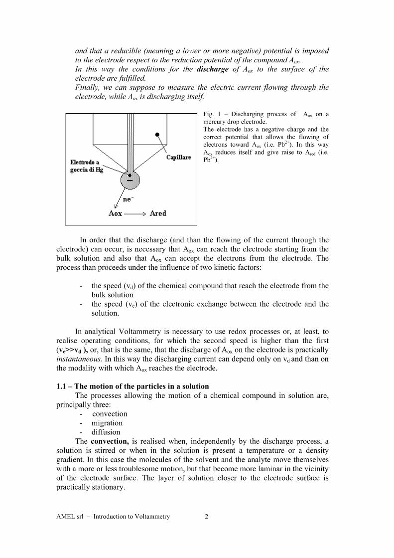
and that a reducible (meaning a lower or more negative) potential is imposed
to the electrode respect to the reduction potential of the compound Aox.
In this way the conditions for the discharge of Aox to the surface of the
electrode are fulfilled.
Finally, we can suppose to measure the electric current flowing through the
electrode, while Aox is discharging itself.
Fig. 1 – Discharging process of Aox on a
mercury drop electrode.
The electrode has a negative charge and the
correct potential that allows the flowing of
electrons toward Aox (i.e. Pb2+
). In this way
Aox reduces itself and give raise to Ared (i.e.
Pb2+
).
In order that the discharge (and than the flowing of the current through the
electrode) can occur, is necessary that Aox can reach the electrode starting from the
bulk solution and also that Aox can accept the electrons from the electrode. The
process than proceeds under the influence of two kinetic factors:
- the speed (vd) of the chemical compound that reach the electrode from the
bulk solution
- the speed (ve) of the electronic exchange between the electrode and the
solution.
In analytical Voltammetry is necessary to use redox processes or, at least, to
realise operating conditions, for which the second speed is higher than the first
(ve>>vd ), or, that is the same, that the discharge of Aox on the electrode is practically
instantaneous. In this way the discharging current can depend only on vd and than on
the modality with which Aox reaches the electrode.
1.1 – The motion of the particles in a solution
The processes allowing the motion of a chemical compound in solution are,
principally three:
- convection
- migration
- diffusion
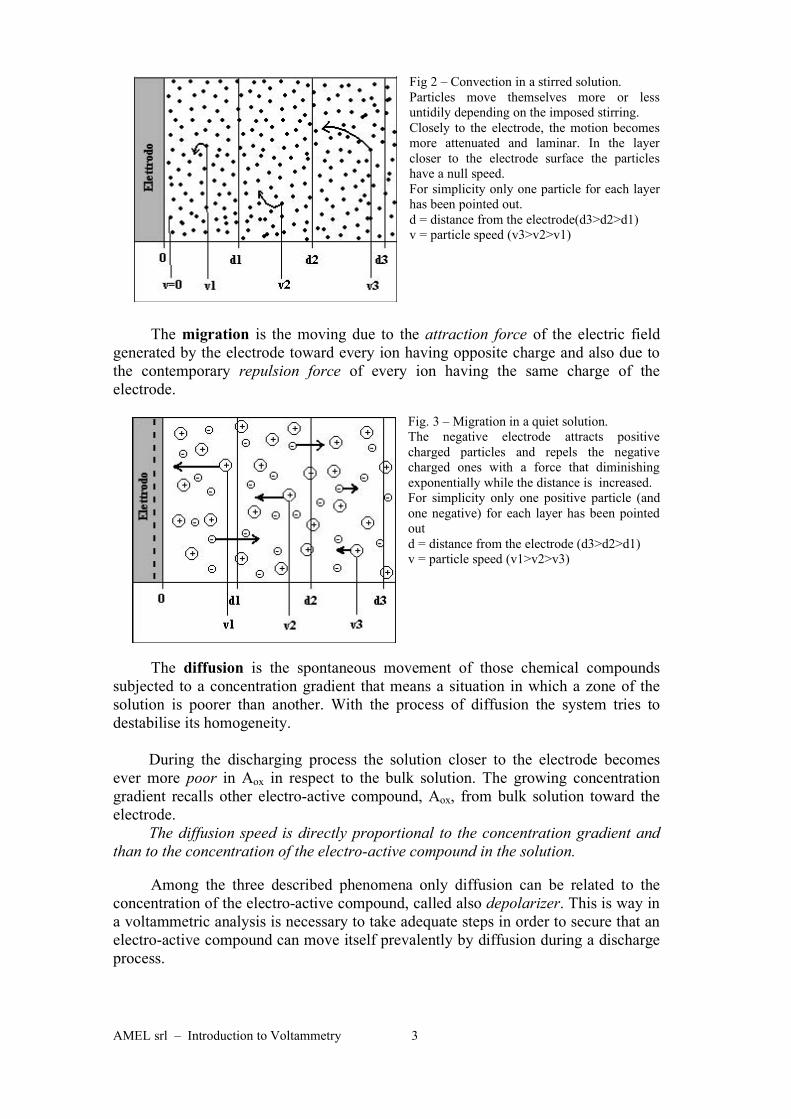
The convection, is realised when, independently by the discharge process, a
solution is stirred or when in the solution is present a temperature or a density
gradient. In this case the molecules of the solvent and the analyte move themselves
with a more or less troublesome motion, but that become more laminar in the vicinity
of the electrode surface. The layer of solution closer to the electrode surface is
practically stationary.
AMEL srl – Introduction to Voltammetry 3
Fig 2 – Convection in a stirred solution.
Particles move themselves more or less
untidily depending on the imposed stirring.
Closely to the electrode, the motion becomes
more attenuated and laminar. In the layer
closer to the electrode surface the particles
have a null speed.
For simplicity only one particle for each layer
has been pointed out.
d = distance from the electrode(d3>d2>d1)
v = particle speed (v3>v2>v1)
The migration is the moving due to the attraction force of the electric field
generated by the electrode toward every ion having opposite charge and also due to
the contemporary repulsion force of every ion having the same charge of the
electrode.
Fig. 3 – Migration in a quiet solution.
The negative electrode attracts positive
charged particles and repels the negative
charged ones with a force that diminishing
exponentially while the distance is increased.
For simplicity only one positive particle (and
one negative) for each layer has been pointed
out
d = distance from the electrode (d3>d2>d1)
v = particle speed (v1>v2>v3)
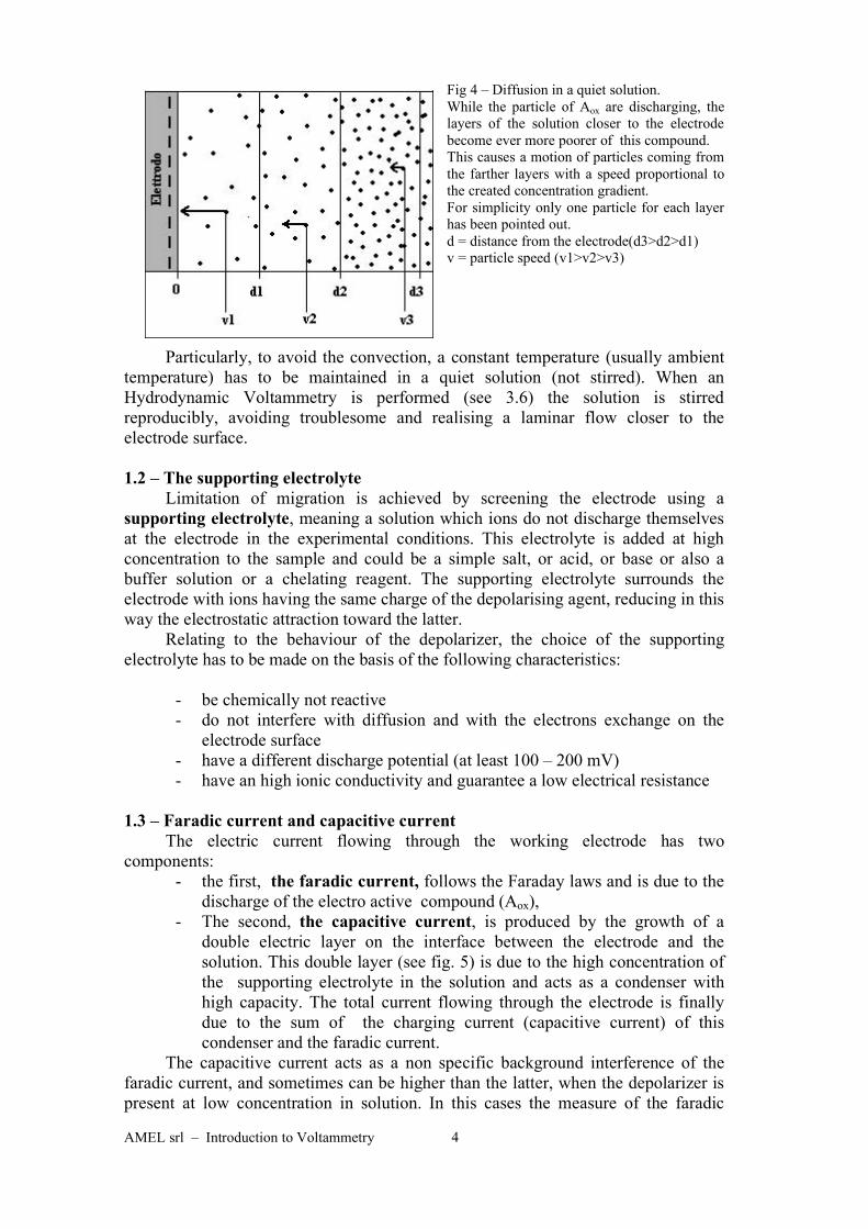
The diffusion is the spontaneous movement of those chemical compounds
subjected to a concentration gradient that means a situation in which a zone of the
solution is poorer than another. With the process of diffusion the system tries to
destabilise its homogeneity.
During the discharging process the solution closer to the electrode becomes
ever more poor in Aox in respect to the bulk solution. The growing concentration
gradient recalls other electro-active compound, Aox, from bulk solution toward the
electrode.
The diffusion speed is directly proportional to the concentration gradient and
than to the concentration of the electro-active compound in the solution.
Among the three described phenomena only diffusion can be related to the
concentration of the electro-active compound, called also depolarizer. This is way in
a voltammetric analysis is necessary to take adequate steps in order to secure that an
electro-active compound can move itself prevalently by diffusion during a discharge
process.
AMEL srl – Introduction to Voltammetry 4
Fig 4 – Diffusion in a quiet solution.
While the particle of Aox are discharging, the
layers of the solution closer to the electrode
become ever more poorer of this compound.
This causes a motion of particles coming from
the farther layers with a speed proportional to
the created concentration gradient.
For simplicity only one particle for each layer
has been pointed out.
d = distance from the electrode(d3>d2>d1)
v = particle speed (v1>v2>v3)
Particularly, to avoid the convection, a constant temperature (usually ambient
temperature) has to be maintained in a quiet solution (not stirred). When an
Hydrodynamic Voltammetry is performed (see 3.6) the solution is stirred
reproducibly, avoiding troublesome and realising a laminar flow closer to the
electrode surface.
1.2 – The supporting electrolyte
Limitation of migration is achieved by screening the electrode using a
supporting electrolyte, meaning a solution which ions do not discharge themselves
at the electrode in the experimental conditions. This electrolyte is added at high
concentration to the sample and could be a simple salt, or acid, or base or also a
buffer solution or a chelating reagent. The supporting electrolyte surrounds the
electrode with ions having the same charge of the depolarising agent, reducing in this
way the electrostatic attraction toward the latter.
Relating to the behaviour of the depolarizer, the choice of the supporting
electrolyte has to be made on the basis of the following characteristics:
- be chemically not reactive
- do not interfere with diffusion and with the electrons exchange on the
electrode surface
- have a different discharge potential (at least 100 – 200 mV)
- have an high ionic conductivity and guarantee a low electrical resistance
1.3 – Faradic current and capacitive current
The electric current flowing through the working electrode has two
components:
- the first, the faradic current, follows the Faraday laws and is due to the
discharge of the electro active compound (Aox),
- The second, the capacitive current, is produced by the growth of a
double electric layer on the interface between the electrode and the
solution. This double layer (see fig. 5) is due to the high concentration of
the supporting electrolyte in the solution and acts as a condenser with
high capacity. The total current flowing through the electrode is finally
due to the sum of the charging current (capacitive current) of this
condenser and the faradic current.
The capacitive current acts as a non specific background interference of the
faradic current, and sometimes can be higher than the latter, when the depolarizer is
present at low concentration in solution. In this cases the measure of the faradic
AMEL srl – Introduction to Voltammetry 5
current is difficult and some electronic adjustment has to be used. That’s why
Polarography (and Voltammetry) is growth, as analytical technique, only after the
progress in the electronic field: so we can now affirm that the development of this
technique is strictly linked to the tentative to electronically overcome problems due
to capacitive current.
Fig. 5 – Simplified double electric layer.
When a negative potential is applied to the
electrode and in the solution the concentration
of positive ions is high, a double electric layer
take place onto the surface of the electrode.
This works just like a condenser.
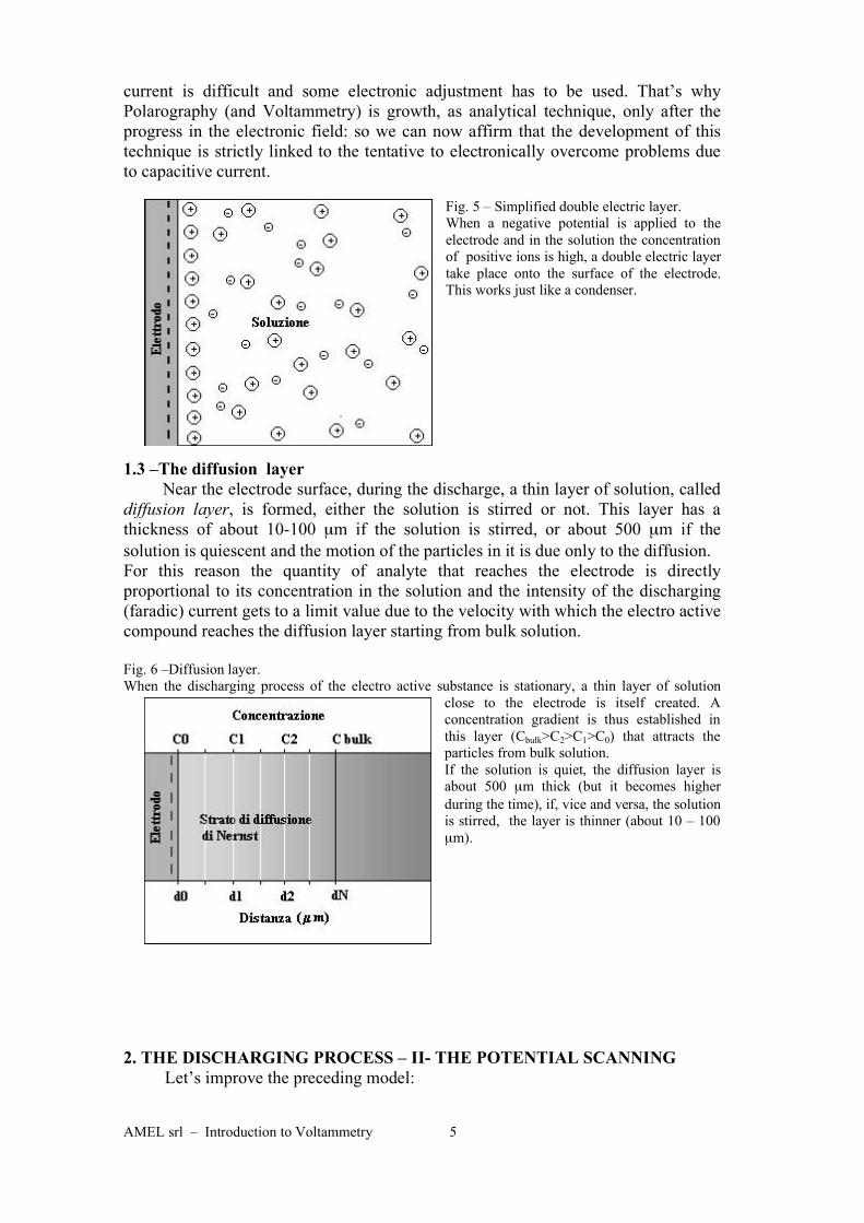
1.3 –The diffusion layer
Near the electrode surface, during the discharge, a thin layer of solution, called
diffusion layer, is formed, either the solution is stirred or not. This layer has a
thickness of about 10-100 µm if the solution is stirred, or about 500 µm if the
solution is quiescent and the motion of the particles in it is due only to the diffusion.
For this reason the quantity of analyte that reaches the electrode is directly
proportional to its concentration in the solution and the intensity of the discharging
(faradic) current gets to a limit value due to the velocity with which the electro active
compound reaches the diffusion layer starting from bulk solution.
Fig. 6 –Diffusion layer.
When the discharging process of the electro active substance is stationary, a thin layer of solution
close to the electrode is itself created. A
concentration gradient is thus established in
this layer (Cbulk>C2>C1>C0) that attracts the
particles from bulk solution.
If the solution is quiet, the diffusion layer is
about 500 µm thick (but it becomes higher
during the time), if, vice and versa, the solution
is stirred, the layer is thinner (about 10 – 100
µm).
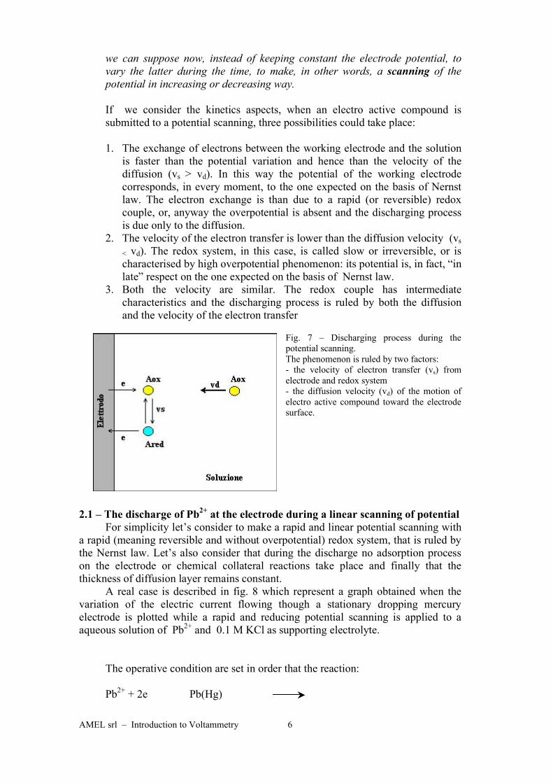
2. THE DISCHARGING PROCESS – II- THE POTENTIAL SCANNING
Let’s improve the preceding model:
AMEL srl – Introduction to Voltammetry 6
we can suppose now, instead of keeping constant the electrode potential, to
vary the latter during the time, to make, in other words, a scanning of the
potential in increasing or decreasing way.
If we consider the kinetics aspects, when an electro active compound is
submitted to a potential scanning, three possibilities could take place:
1. The exchange of electrons between the working electrode and the solution
is faster than the potential variation and hence than the velocity of the
diffusion (vs > vd). In this way the potential of the working electrode
corresponds, in every moment, to the one expected on the basis of Nernst
law. The electron exchange is than due to a rapid (or reversible) redox
couple, or, anyway the overpotential is absent and the discharging process
is due only to the diffusion.
2. The velocity of the electron transfer is lower than the diffusion velocity (vs
< vd). The redox system, in this case, is called slow or irreversible, or is
characterised by high overpotential phenomenon: its potential is, in fact, “in
late” respect on the one expected on the basis of Nernst law.
3. Both the velocity are similar. The redox couple has intermediate
characteristics and the discharging process is ruled by both the diffusion
and the velocity of the electron transfer
Fig. 7 – Discharging process during the
potential scanning.
The phenomenon is ruled by two factors:
- the velocity of electron transfer (vs) from
electrode and redox system
- the diffusion velocity (vd) of the motion of
electro active compound toward the electrode
surface.
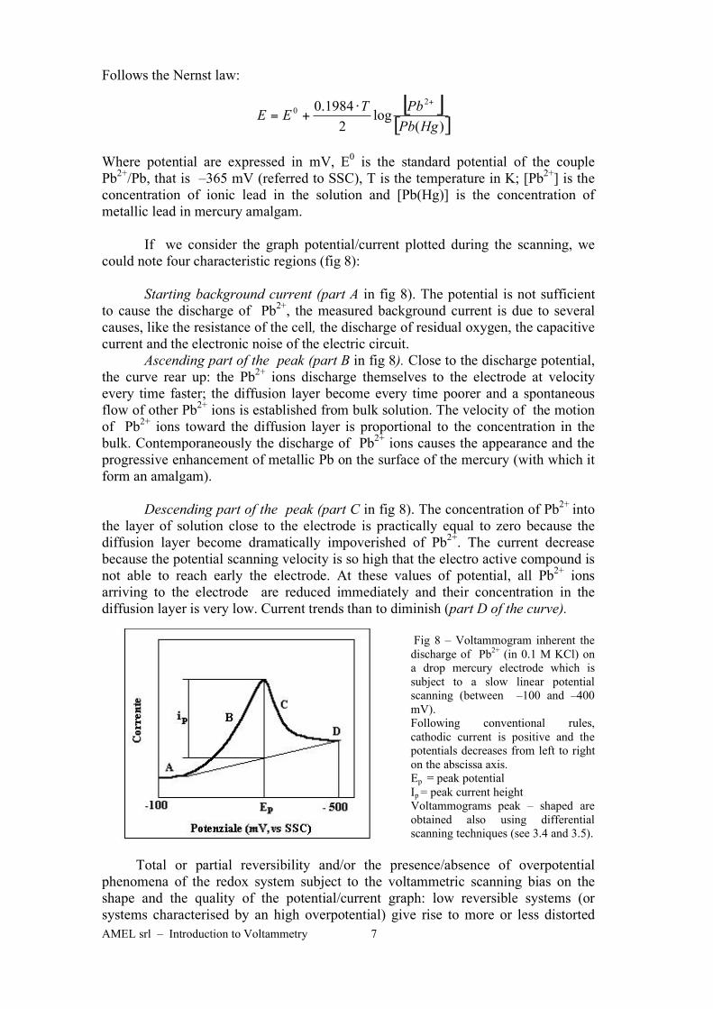
2.1 – The discharge of Pb2+
at the electrode during a linear scanning of potential
For simplicity let’s consider to make a rapid and linear potential scanning with
a rapid (meaning reversible and without overpotential) redox system, that is ruled by
the Nernst law. Let’s also consider that during the discharge no adsorption process
on the electrode or chemical collateral reactions take place and finally that the
thickness of diffusion layer remains constant.
A real case is described in fig. 8 which represent a graph obtained when the
variation of the electric current flowing though a stationary dropping mercury
electrode is plotted while a rapid and reducing potential scanning is applied to a
aqueous solution of Pb2+
and 0.1 M KCl as supporting electrolyte.
The operative condition are set in order that the reaction:
Pb2+
+ 2e Pb(Hg)
AMEL srl – Introduction to Voltammetry 7
Follows the Nernst law:
Where potential are expressed in mV, E0 is the standard potential of the couple
Pb2+
/Pb, that is –365 mV (referred to SSC), T is the temperature in K; [Pb2+
] is the
concentration of ionic lead in the solution and [Pb(Hg)] is the concentration of
metallic lead in mercury amalgam.
If we consider the graph potential/current plotted during the scanning, we
could note four characteristic regions (fig 8):
Starting background current (part A in fig 8). The potential is not sufficient
to cause the discharge of Pb2+
, the measured background current is due to several
causes, like the resistance of the cell, the discharge of residual oxygen, the capacitive
current and the electronic noise of the electric circuit.
Ascending part of the peak (part B in fig 8). Close to the discharge potential,
the curve rear up: the Pb2+
ions discharge themselves to the electrode at velocity
every time faster; the diffusion layer become every time poorer and a spontaneous
flow of other Pb2+
ions is established from bulk solution. The velocity of the motion
of Pb2+
ions toward the diffusion layer is proportional to the concentration in the
bulk. Contemporaneously the discharge of Pb2+
ions causes the appearance and the
progressive enhancement of metallic Pb on the surface of the mercury (with which it
form an amalgam).
Descending part of the peak (part C in fig 8). The concentration of Pb2+
into
the layer of solution close to the electrode is practically equal to zero because the
diffusion layer become dramatically impoverished of Pb2+
. The current decrease
because the potential scanning velocity is so high that the electro active compound is
not able to reach early the electrode. At these values of potential, all Pb2+
ions
arriving to the electrode are reduced immediately and their concentration in the
diffusion layer is very low. Current trends than to diminish (part D of the curve).
Fig 8 – Voltammogram inherent the
discharge of Pb2+
(in 0.1 M KCl) on
a drop mercury electrode which is
subject to a slow linear potential
scanning (between –100 and –400
mV).
Following conventional rules,
cathodic current is positive and the
potentials decreases from left to right
on the abscissa axis.
Ep = peak potential
Ip = peak current height
Voltammograms peak – shaped are
obtained also using differential
scanning techniques (see 3.4 and 3.5).
Total or partial reversibility and/or the presence/absence of overpotential
phenomena of the redox system subject to the voltammetric scanning bias on the
shape and the quality of the potential/current graph: low reversible systems (or
systems characterised by an high overpotential) give rise to more or less distorted
[ ][ ])(
log2
1984.0 20
HgPb
PbTEE
+!
+=
AMEL srl – Introduction to Voltammetry 8
peaks, but completely irreversible systems (or systems characterised by a very high
overpotential) cannot give rise to a significant peak.
2.2 – Peak potential
The higher point of a peak correspond to the point in which the half quantity
of Pb2+
ions that reach the electrode discharge themselves, then the ratio Pb2+
/Pb(Hg)
at the electrode/solution interface become equal to 1. It can be demonstrated that the
measured potential is not so far from the redox potential of the redox couple
(obviously, in the supporting electrolyte solution…). The potential peak is than the
analytical parameter that allows to make a qualitative characterisation a redox
couple in a solution..
2.3 - Peak current height - Peak height (hpeak)
The peak current height is proportional to the concentration of the electro
active compound in the solution:
ip = K![Pb2+
]
and than correspond to the analytical parameter useful for a quantitative analysis.
AMEL srl – Manuale di Voltammetria 9
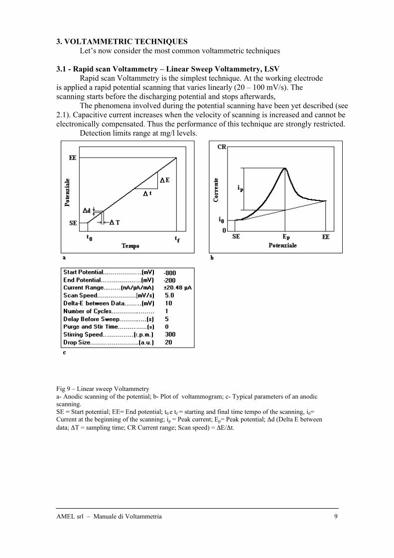
3. VOLTAMMETRIC TECHNIQUES
Let’s now consider the most common voltammetric techniques
3.1 - Rapid scan Voltammetry – Linear Sweep Voltammetry, LSV
Rapid scan Voltammetry is the simplest technique. At the working electrode
is applied a rapid potential scanning that varies linearly (20 – 100 mV/s). The
scanning starts before the discharging potential and stops afterwards,
The phenomena involved during the potential scanning have been yet described (see
2.1). Capacitive current increases when the velocity of scanning is increased and cannot be
electronically compensated. Thus the performance of this technique are strongly restricted.
Detection limits range at mg/l levels.
Fig 9 – Linear sweep Voltammetry
a- Anodic scanning of the potential; b- Plot of voltammogram; c- Typical parameters of an anodic
scanning.
SE = Start potential; EE= End potential; t0 e tf = starting and final time tempo of the scanning, i0=
Current at the beginning of the scanning; ip = Peak current; Ep= Peak potential; !d (Delta E between
data; !T = sampling time; CR Current range; Scan speed) = !E/!t.
AMEL srl – Manuale di Voltammetria 10
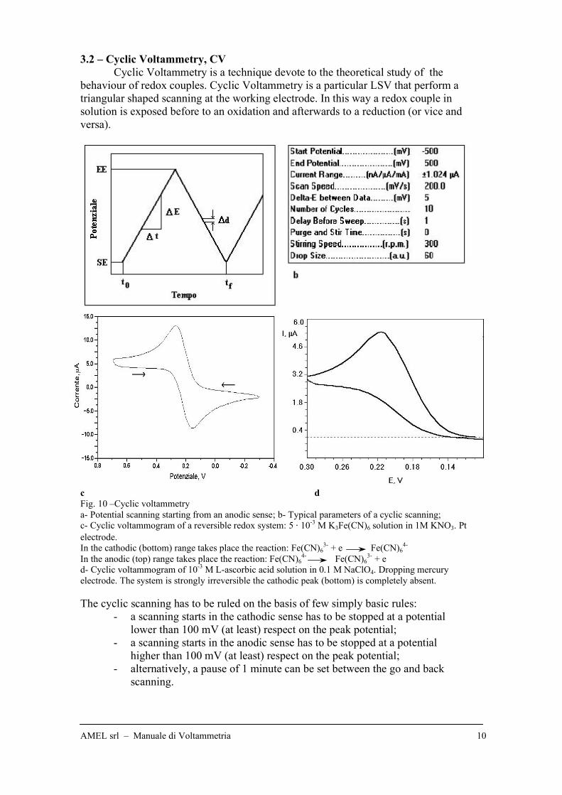
3.2 – Cyclic Voltammetry, CV
Cyclic Voltammetry is a technique devote to the theoretical study of the
behaviour of redox couples. Cyclic Voltammetry is a particular LSV that perform a
triangular shaped scanning at the working electrode. In this way a redox couple in
solution is exposed before to an oxidation and afterwards to a reduction (or vice and
versa).
c d
Fig. 10 –Cyclic voltammetry
a- Potential scanning starting from an anodic sense; b- Typical parameters of a cyclic scanning;
c- Cyclic voltammogram of a reversible redox system: 5 " 10-3
M K3Fe(CN)6 solution in 1M KNO3. Pt
electrode.
In the cathodic (bottom) range takes place the reaction: Fe(CN)63-
+ e Fe(CN)64-
In the anodic (top) range takes place the reaction: Fe(CN)64-
Fe(CN)63-
+ e
d- Cyclic voltammogram of 10-3
M L-ascorbic acid solution in 0.1 M NaClO4. Dropping mercury
electrode. The system is strongly irreversible the cathodic peak (bottom) is completely absent.
The cyclic scanning has to be ruled on the basis of few simply basic rules:
- a scanning starts in the cathodic sense has to be stopped at a potential
lower than 100 mV (at least) respect on the peak potential;
- a scanning starts in the anodic sense has to be stopped at a potential
higher than 100 mV (at least) respect on the peak potential;
- alternatively, a pause of 1 minute can be set between the go and back
scanning.
AMEL srl – Manuale di Voltammetria 11
The plot of a cyclic voltammetry consist on a close curve: reversible redox couples
show both as cathodic and anodic peak, while irreversible redox systems show only
one peak.
The following relations can be useful to establish the standard potential of a
reversible redox couple and the number of electrons involved in the discharge
process:
and
where Epa= anodic peak potential , in mV e Epc= cathodic peak potential.
Generally this technique is not used for quantitative analysis because its poor
sensitivity
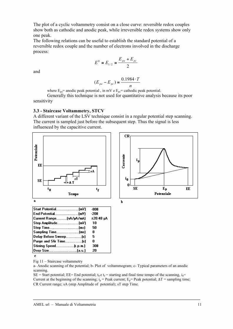
3.3 - Staircase Voltammetry, STCV
A different variant of the LSV technique consist in a regular potential step scanning.
The current is sampled just before the subsequent step. Thus the signal is less
influenced by the capacitive current.
Fig 11 – Staircase voltammetry
a- Anodic scanning of the potential; b- Plot of voltammogram; c- Typical parameters of an anodic
scanning.
SE = Start potential; EE= End potential; t0 e tf = starting and final time tempo of the scanning, i0=
Current at the beginning of the scanning; ip = Peak current; Ep= Peak potential; !T = sampling time;
CR Current range; sA (step Amplitude of potential); sT step Time.
n
TEE pcpa
!"#
1984.0)(
22/1
0 pcpa EEEE
+!!
AMEL srl – Manuale di Voltammetria 12
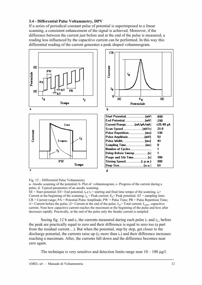
3.4 - Differential Pulse Voltammetry, DPV
If a series of periodical constant pulse of potential is superimposed to a linear
scanning, a consistent enhancement of the signal is achieved. Moreover, if the
difference between the current just before and at the end of the pulse is measured, a
reading less influenced by the capacitive current can be performed. In this way this
differential reading of the current generates a peak shaped voltammogram.
Fig. 12 – Differential Pulse Voltammetry
a- Anodic scanning of the potential; b- Plot of voltammogram; c- Progress of the current during a
pulse; d- Typical parameters of an anodic scanning.
SE = Start potential; EE= End potential; t0 e tf = starting and final time tempo of the scanning, i0=
Current at the beginning of the scanning; ip = Peak current; Ep= Peak potential; !T = sampling time;
CR = Current range; PA = Potential Pulse Amplitude; PW = Pulse Time; PR = Pulse Repetition Time;
i1= Current before the pulse; i2= Current at the end of the pulse; Itot= Total current; Icapac= capacitive
current. Note how capacitive current reaches the maximum at the beginning of the pulse and how after
decreases rapidly. Practically, at the end of the pulse only the faradic current is sampled.
Seeing fig. 12 b and c, the currents measured during each pulse i1 and i2,, before
the peak are practically equal to zero and their difference is equal to zero too (a part
from the residual current…). But when the potential, step by step, get closer to the
discharge potential, the currents raise up (i2 more than i1) and their difference increases
reaching a maximum. After, the currents fall down and the difference becomes near
zero again.
The technique is very sensitive and detection limits range near 10 – 100 µg/l.
AMEL srl – Manuale di Voltammetria 13
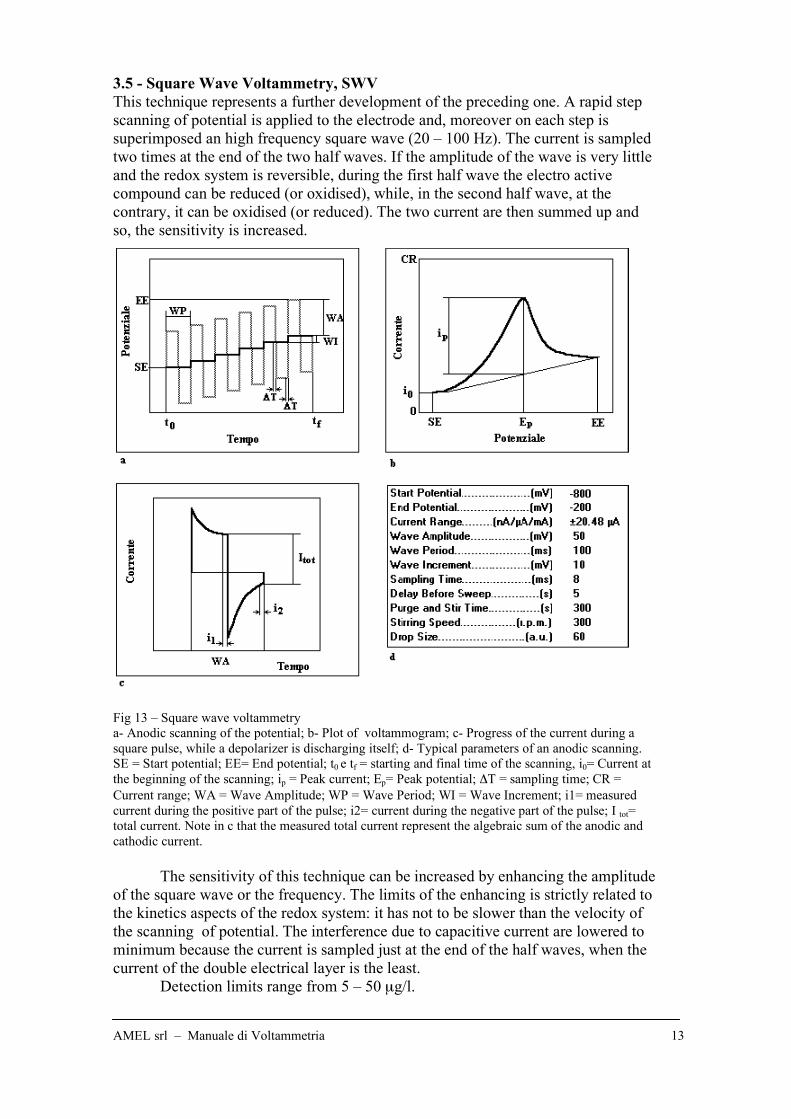
3.5 - Square Wave Voltammetry, SWV
This technique represents a further development of the preceding one. A rapid step
scanning of potential is applied to the electrode and, moreover on each step is
superimposed an high frequency square wave (20 – 100 Hz). The current is sampled
two times at the end of the two half waves. If the amplitude of the wave is very little
and the redox system is reversible, during the first half wave the electro active
compound can be reduced (or oxidised), while, in the second half wave, at the
contrary, it can be oxidised (or reduced). The two current are then summed up and
so, the sensitivity is increased.
Fig 13 – Square wave voltammetry
a- Anodic scanning of the potential; b- Plot of voltammogram; c- Progress of the current during a
square pulse, while a depolarizer is discharging itself; d- Typical parameters of an anodic scanning.
SE = Start potential; EE= End potential; t0 e tf = starting and final time of the scanning, i0= Current at
the beginning of the scanning; ip = Peak current; Ep= Peak potential; !T = sampling time; CR =
Current range; WA = Wave Amplitude; WP = Wave Period; WI = Wave Increment; i1= measured
current during the positive part of the pulse; i2= current during the negative part of the pulse; I tot=
total current. Note in c that the measured total current represent the algebraic sum of the anodic and
cathodic current.
The sensitivity of this technique can be increased by enhancing the amplitude
of the square wave or the frequency. The limits of the enhancing is strictly related to
the kinetics aspects of the redox system: it has not to be slower than the velocity of
the scanning of potential. The interference due to capacitive current are lowered to
minimum because the current is sampled just at the end of the half waves, when the
current of the double electrical layer is the least.
Detection limits range from 5 – 50 µg/l.
AMEL srl – Manuale di Voltammetria 14
3.6 – Hydrodynamic Voltammetry
Rotating Disk Voltammetry, RDV - Rotating Ring-Disk Voltammetry, RRDV
In the hydrodynamic techniques the scanning of the potential takes place
while the solution is in motion toward the electrode. In this way the solution closed
to the Nernst (practically quiet) layer is continuously renewed.
The motion is actuated in 3 different ways:
- the electrode is stationary and the solution is stirred. This technique has
low reproducibility and is practically not used.
- the solid electrode rotates around the own axis, the solution is than stirred.
The electrode is a disk or a disk coupled with a ring.
- The solution flows into a tubular electrode at constant velocity. This
system is used as voltammetric detector in HPLC.
The obtained voltammogram is a wave. In fact (see fig. 15 b) the plot
potential /current is characterised by an initial residual current (A) that grows up just
in correspondence (B) of the discharging potential (E1/2, half wave potential).
Successively the current increases, but slowly until a stationary level is reached. At
this values of potential the ions reaching the electrode discharge themselves
immediately, thus the concentration of the analyte in the diffusion layer is practically
null. The continuos flowing of ions onto the diffusion layer, due to the stirring,
maintains a constant current (C)
Fig. 15 – Hydrodynamic voltammetry
a- Rotating electrode; b- typical hydrodynamic voltammogram wave shaped.
3.7 - Stripping Voltammetry, SV
Anodic Stripping Voltammetry, ASV – Cathodic Stripping Voltammetry, CSV
Some metals forms an amalgam with the working electrode and some anions
forms insoluble salts with it. The stripping voltammetry is based upon these
properties.
The technique follows two main steps:
- A pre-concentration of the analyte onto the electrode
- The successive stripping of the cumulate compound onto the electrode
toward the solution.
AMEL srl – Manuale di Voltammetria 15
The stripping takes place during a scanning with the usual techniques (linear
or differential pulsed or square wave scanning).
The usual working electrode is a dropping (or a film) mercury and the most
common technique is the anodic stripping, meaning that a negative potential is
applied to the electrode and the cations are discharged as metallic atoms into the
mercury (amalgam). Successively the metal atoms are oxidised again, during an
anodic scanning of potential. During the scanning of the potential, the current is
measured and plotted, so the resulting voltammogram is a peak shaped graphic. The
position and the heght of this peak are related, respectively, to the type and to the
concentration of the analyte.
The analysis of anions on mercury takes place following a inverse way: first
mercury oxidise itself and forms a insoluble salt with the anion and after, by applying
a cathodic scanning, mercury reduce itself and the anion come back in solution.
Exemple:
2Hg + 2Cl- Hg2Cl2 + 2e pre-concentration
Hg2Cl2 + 2e 2Hg + 2Cl- reducing (cathodic) scanning
This technique allows to considerably enhance the sensitivity because during
the pre-concentration step a great quantity of analyte in a small volume of electrode
(the mercury drop) and the measured stripping currents are greater than the ones
obtained using a non accumulative voltammetric techniques.
In this way detection limits below µg/l are achieved.
Fig. 16 – Anodic stripping voltammetry in a solution containing Pb2+
, Cd2+
e Cu2+
.
a- Potential scanning ; b- Voltammogram.
The scanning in the figure is linear but could be also a differential pulse or square wave ones.
Deposition potential = Starting potential (SE) = -800 mV; End potential (EE) = +300 mV; deposition
time = 60 sec. For the other parameters see the relatives techniques (LSV, DPV or SWV).
3.8 - Adsorbtive Voltammetry, AdV - Adsorbtive Stripping Voltammetry, AdSV
Some metallic complex and some organic substances are adsorbed onto the
surface of the electrode at specific potential. This phenomenon can be useful
exploited when metals do not form amalgam onto the mercury, but form complex
that can be adsorbed onto the latter and analysed with a direct scanning or a stripping
technique. The detection limits are below the µg/l, while the linear range is often
short.
AMEL srl – Manuale di Voltammetria 16
3.9 - Adsorbtive Stripping Tensammetry, AdST
Some organic substances, like surfactants, are not electrically active, but
show an electrical activity at the solution/electrode interface, while a pulsed or a
rapid linear scanning is applied to the electrode. In correspondence of the
desorbtion/adsorbtion potential a tensammetric peak is obtained. The analyte can be
so analysed at mg/l levels.
3.10 – Polarographic techniques
Classical Polarography, developed by Heyrowsky, is now an obsolete
technique. In the following pages are reported only few techniques that are already
used.
3.10.1 - Rapid DC Polarography
The mercury drops fall down, rhythmically, from the capillary with a imposed
rhythm, while a linear scanning is imposed to the electrode. The obtained polarogram
is a wave characterised by strong oscillations due to the rhythmic falling of the drop
(that means a rhythmic interruption of the electrical circuit).
a b Fig. 17 - Rapid DC polarography.
a- Rapid DC polarogram of Cd2+
e Pb2+
(50 mg/l each) in 0.1 M KCl solution.
b- Polarogram of the same solution plotted as first derivative.
3.10.2 - Sampled (or Test) DC Polarography - Staircase Polarography
The interference of capacitive current in the previous technique is strong. Capacitive current reach its maximum in the first moments of life of the drop and
goes to the minimum just before the drop fall down.
In this technique, the potential is increased (or decreased) at the beginning by
a step and maintained constant during the life of each drop. The current is measured
in the last moment of life of the drop. A stepped wave polarogram, with a smaller
noise, is thus obtained.
AMEL srl – Manuale di Voltammetria 17
3.10.3 - Normal Pulse Polarography, NPP - Differential Pulse Polarography,
DPP
Pulsed techniques allow to reduce the capacitive current. In the Normal Pulse
Polarography a potential pulse is imposed to the drop during its last moment of life.
The pulse height is linearly increased during the time. In the Differential Pulse
Polarography the potential pulse is constant but is over imposed to a linear
scanning of the potential (see DPV).
The polarogram is a wave in NPP and a peak in DPP and the height of both
are related to the concentration of the analyte.
DPP was been, for a long time, the most used technique and it has allowed to
develop the first procedures and is the basis for the further developments of the
analytical voltammetric techniques.
Fig. 18 - Potential scanning during : a- Staircase Polarography, b- NPP c- DPP
SE = Start potential; EE= End potential; ; t0 e tf = starting and final time of the scanning ; !T = Sampling Time;
tg = dropping time; sA: height of potential step.
AMEL srl – Manuale di Voltammetria 18
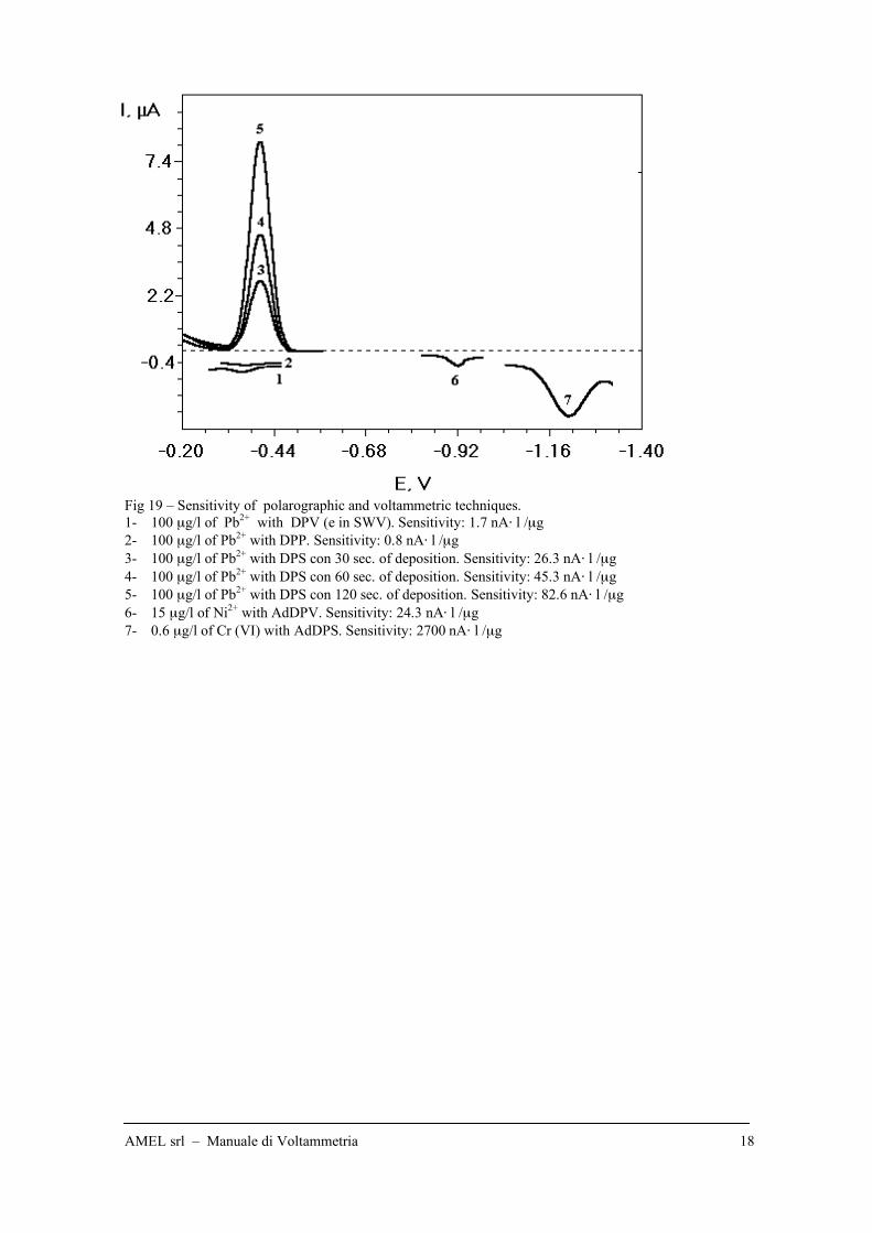
Fig 19 – Sensitivity of polarographic and voltammetric techniques.
1- 100 µg/l of Pb2+
with DPV (e in SWV). Sensitivity: 1.7 nA" l /µg
2- 100 µg/l of Pb2+
with DPP. Sensitivity: 0.8 nA" l /µg
3- 100 µg/l of Pb2+
with DPS con 30 sec. of deposition. Sensitivity: 26.3 nA" l /µg
4- 100 µg/l of Pb2+
with DPS con 60 sec. of deposition. Sensitivity: 45.3 nA" l /µg
5- 100 µg/l of Pb2+
with DPS con 120 sec. of deposition. Sensitivity: 82.6 nA" l /µg
6- 15 µg/l of Ni2+
with AdDPV. Sensitivity: 24.3 nA" l /µg
7- 0.6 µg/l of Cr (VI) with AdDPS. Sensitivity: 2700 nA" l /µg
AMEL srl – Introduction to Voltammetry 20
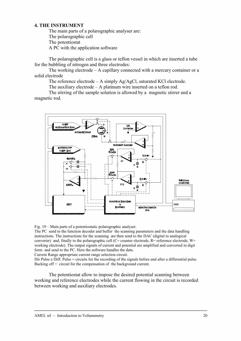
4. THE INSTRUMENT
The main parts of a polarographic analyser are:
The polarographic cell
The potentiostat
A PC with the application software
The polarographic cell is a glass or teflon vessel in which are inserted a tube
for the bubbling of nitrogen and three electrodes:
The working electrode – A capillary connected with a mercury container or a
solid electrode
The reference electrode – A simply Ag/AgCl, saturated KCl electrode.
The auxiliary electrode – A platinum wire inserted on a teflon rod.
The stirring of the sample solution is allowed by a magnetic stirrer and a
magnetic rod.
Fig. 19 – Main parts of a potentiostatic polarographic analyser.
The PC send to the function decoder and buffer the scanning parameters and the data handling
instructions. The instructions for the scanning are then send to the DAC (digital to analogical
converter) and, finally to the polarographic cell (C= counter electrode, R= reference electrode, W=
working electrode). The output signals of current and potential are amplified and converted in digit
form and send to the PC. Here the software handles the data.
Current Range appropriate current range selection circuit.
Dir Pulse e Diff. Pulse = circuits for the recording of the signals before and after a differential pulse.
Backing off = circuit for the compensation of the background current.
The potentiostat allow to impose the desired potential scanning between
working and reference electrodes while the current flowing in the circuit is recorded
between working and auxiliary electrodes.
AMEL srl – Introduction to Voltammetry 21
The PC is interfaced to measuring system and the software has the following
functions:
- send to the potentiostatic analyser the scanning parameters
- check if the execution of the scanning is correct or not
- handle the output data (current and potential).
4.1 – Working electrode
The operating range of a potential scanning depends on:
- kind of solvent
- chemical structure of the electrode
- surface characteristics of the electrode
- supporting solution
- sensitivity of the instrument
In water solution this range restricted in the cathodic side by the hydrogen
discharge:
2H+ + 2 e H2
While, in the anodic side by the oxidation of water:
O2 + 4H+ + 4 e
2H2O
or by the discharge of the constituent material of the electrode i. e.
Hg2+
+ 2e Hg
The potentials of the two discharging processes above described, can shift
considerably depending on the overpotential phenomena due to chemical structure of
the electrode.
Let’s now consider the most important materials for electrodes.
4.2 – Mercury electrode
Mercury is the best metal for cathodic scanning because of the large
overpotential that the hydrogen discharge undergo on this element. The density of the
discharge of the hydrogen on mercury is 109 time less than the platinum and gold
ones. On mercury the hydrogen discharge occur at -1 V (Vs SSC, in acidic solution)
or at – 2 V (Vs SSC, in alkaline solution), instead of a theoretical potential of –0.2 V
(Vs SSC).
In the anodic side the operating limit is restricted by the discharge of mercury
itself:
Hg22+
+ 2 e 2Hg
Hg2+
+ 2 e Hg
Practically, it is impossible use the mercury electrode above 0.3 V (Vs. SSC).
Another advantage on the use of mercury as electrode is due to the
opportunity of eliminate a drop of this element at the end of the scanning. In this
way the surface of the electrode can be renewed before each analysis.
AMEL srl – Introduction to Voltammetry 22
On the other hand, mercury is a toxic metal, rather volatile. Anyway the
modern instruments are perfectly sealed and the volume of the mercury container is
very small.
The latest version of this electrode, the Static Mercury Dropping Electrode,
SMDE is a capillary (0.15 – 0.2 mm ID) connected to the mercury container. A
valve, operated by a PC, adjust the dimension of the drop, while a platinum wire
ensure the electrical connection with the electrical circuit. The older DME (Dropping Mercury Electrode), in which the mercury flowed down simply by gravity
or the HMDE (Hanging Mercury Dropping Electrode), in which a piston developed the drop are not in
use. The SMDE (Long Lasting Sessile Dropping Mercury Electrode) is still used when then scanning
has to be prolonged at values smaller than –1.4 V. At these potentials the drop on the SMDE inclines
to fall down for electrostatic phenomena.
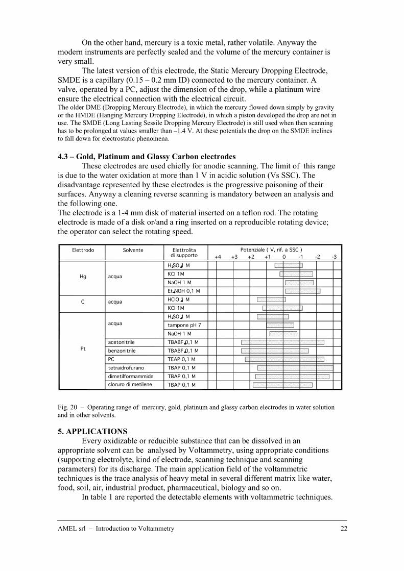
4.3 – Gold, Platinum and Glassy Carbon electrodes
These electrodes are used chiefly for anodic scanning. The limit of this range
is due to the water oxidation at more than 1 V in acidic solution (Vs SSC). The
disadvantage represented by these electrodes is the progressive poisoning of their
surfaces. Anyway a cleaning reverse scanning is mandatory between an analysis and
the following one.
The electrode is a 1-4 mm disk of material inserted on a teflon rod. The rotating
electrode is made of a disk or/and a ring inserted on a reproducible rotating device;
the operator can select the rotating speed.
Fig. 20 – Operating range of mercury, gold, platinum and glassy carbon electrodes in water solution
and in other solvents.
5. APPLICATIONS
Every oxidizable or reducible substance that can be dissolved in an
appropriate solvent can be analysed by Voltammetry, using appropriate conditions
(supporting electrolyte, kind of electrode, scanning technique and scanning
parameters) for its discharge. The main application field of the voltammetric
techniques is the trace analysis of heavy metal in several different matrix like water,
food, soil, air, industrial product, pharmaceutical, biology and so on.
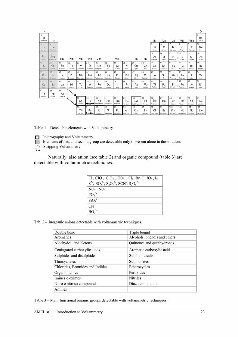
In table 1 are reported the detectable elements with voltammetric techniques.
Elettrodo Solvente
H SO 1 M
tampone pH 7
acetonitrile
benzonitrile
PC
tetraidrofurano
dimetilformammide
cloruro di metilene
acqua
Elettrolita
+4
Pt
acquaHg
C acqua
-1 -2 -3
Potenziale ( V, rif. a SSC )
+3 +2 +1 0di supporto
KCI 1M
NaOH 1 M
Et NOH 0,1 M
HCIO 1 M
KCI 1M
H SO 1 M
NaOH 1 M
TBABF 0,1 M
TBABF 0,1 M
TEAP 0,1 M
TBAP 0,1 M
TBAP 0,1 M
TBAP 0,1 M
AMEL srl – Introduction to Voltammetry 23
Table 1 – Detectable elements with Voltammetry
Polarography and Voltammetry
Elements of first and second group are detectable only if present alone in the solution.
Stripping Voltammetry
Naturally, also anion (see table 2) and organic compound (table 3) are
detectable with voltammetric techniques.
Cl
-, ClO
-, ClO2
-, ClO3
-, Cl2, Br
-, I
-, IO3
-, I2
S2-
, SO3
2-, S2O3
2-, SCN
-, S2O8
2-
NO2-, NO3
-
PO43-
SiO32-
CN-
BO33-
Tab. 2 - Inorganic anions detectable with voltammetric techniques.
Double bond Triple bound
Aromatics Alcohols, phenols and ethers
Aldehydes and Ketons Quinones and quinhydrones
Coniugated carboxylic acids Aromatic carboxylic acids
Sulphides and disulphides Sulphonic salts
Thiocyanates Sulphonates
Chlorides, Bromides and Iodides Etherocycles
Organomellics Peroxides
Imines e oximes Nitriles
Nitro e nitroso compounds Diazo compounds
Amines
Table 3 – Main functional organic groups detectable with voltammetric techniques.
H
Li Be
Na Mg
K Ca Sc Ti
Rb Sr
Cs Ba
Y
La Hf
Zr
AcRaFr
Ta
Nb
V Cr
Mo
W Re
Tc
Mn
Os
Ru
Fe Co
Rh
Ir Pt
Pd
Ni Cu
Ag
Au
Zn
Cd
Hg Tl
In
Ga
Pb
Sn
Ge
Bi
Sb
As
Al
B C N
PSi
O
S Cl
F Ne
Ar
He
KrBrSe
Te I Xe
Po At Rn
Ce Pr Nd Pm Sm
PuNpUPaTh
Eu Gd
Am Cm
Tb
Bk Cf
Dy Lu
Lw
Yb
NoMd
TmEr
FmEs
Ho
1
3 4
1211
19 20 21
3837 39
5655
87 88 89
57 72
22 23 24
40 41 42
73 74
25 26 27
43 44 45
75 76 77 78 79 80
46 47 48
28 29 30 31 32 33 34 35
49 50 51
81 82 83
52 53 54
84 85 86
36
5 6 7 8 9
13 14 15 16 17
2
10
18
58 59 60 61
90 91 92 93
62
94
63 64 65
95 96 97
66
98 99
67 68
100
69 70
101 102
71
103
Iridio
Manganese
Ia
IIa
IIIb IVb Vb VIb VIIb VIII Ib IIb
IIIa IVa Va VIa VIIa
O
Hydrogen
Lithium Beryllium
Sodium Magnesium
Potassium Calcium
Rubidium Strontium
Cesium Barium
Francium Radium Actinium
Lanthanum
Yttrium
Scandium Titanium
Zirconium
Hafnium
Vanadium
Columbium
Tantalum
Chromium
Molybdenum
Tungsten Rhenium
Technetium
Osmium
Ruthenium Rhodium
CobaltIron Nickel
Palladium
Platinum
Silver
Gold Mercury
Cadmium
ZincCopper
Thallium Lead
Indium Tin
Gallium Germanium
Bismuth Polonium
TelluriumAntimony
Arsenic Selenium
Radon
XenonIodine
Astatine
Bromine Krypton
ArgonChlorine
Fluorine Neon
Helium
Boron Carbon Nitrogen Oxigen
SulfurPhosphorusSiliconAluminum
Cerium Neodymium Samarium
UraniumThorium Neptunium Plutonium
Promethium Europium Gadolinium
Americium Curium Berkelium
Terbium Dysprosium
Californium
Holmium
Einsteinium
Erbium
Fermium
Lutetium
Lawrencium
YtterbiumThulium
Mendelevium Nobelium
AMEL srl – Introduction to Voltammetry 24
6. COMPARING VOLTAMMETRY WITH ATOMIC ABSORPTION
SPECTROPHOTOMETRY AND INDUCTIVELY COUPLED PLASMA
SPECTROMETRY
Detection limits and reproducibility of the voltammetric techniques are
comparable with those of Graphite Furnace Atomic Absorption Spectrophotometry
and Inductively Coupled Plasma Spectrometry.
Voltammetry is a electrochemical technique, otherwise the others are optical
techniques.
Optical techniques allow to analyse only metals (and also sulphur and
phosphorous), in solution, while voltammetric techniques allow to analyse also
oxidizable or reducible anions and organic compounds.
Optical techniques allow to analyse total metals, while voltammetric
techniques allow to analyse also metals at different oxidation numbers (i. e. Cr (III)
and Cr(VI), Fe(II) and Fe(III), As(III) and As(V) ).
The spare parts and the costs of a single analysis using optical techniques are
very high, while the Voltammetry is cheaper.
GFAAS needs an accurate adjusting of the analytical method when the
sample matrix is rich in compounds. GFAAS needs therefore very expert analysts
and also a great number of lamps (virtually one for each detectable element). For a
better reproducibility of GFAAS an automatic sampler and injection system is
strictly necessary. Furthermore GFAAS needs a frequent replacement of graphite
tubes and a lot of waste of inert gas (argon).
ICP and ICP-MS suffer for a great waste of argon and for necessity to use
very diluted solutions. ICP-MS needs very expert analysts, principally for the mass
spectrometry. Furthermore the injection system of a ICP is very easily getting dirty
or broken and also is very expensive.
Voltammetric techniques need analysts specialised in electrochemistry and
don not allow to analyse metals of first and second group (Na, K, Li, Ca, Mg, Ba, Sr
…). Furthermore it’s not possible to use automatic sampler. The most replaceable
part is the capillary, but, anyway the spare parts of a Voltammeter are cheaper than
the optical techniques ones. Solutions to be analysed must have a pH lower than 10
and higher than 1 to save the functionality of the capillary. At the moment of the
analysis a supporting solution has to be added to the sample to adjust the reaction
environment and also the discharging condition of the analyte. The times for an
analysis is higher in Voltammetry, but the technique is not destructive and the
sample can be analysed for several time and different analytes. Mercury is a toxic
pollutant and must be recovered in a proper way.
Sensitivity for some elements like Pb, Cd and Se is greater in Voltammetry
than in Optical techniques. And some element. like i.e. Ni, can be analysed in sea
water only using Voltammetry.
The correct analytical method for Voltammetric analysis is the standard
addition method (single or multiple); this allows to compensate the matrix effect of
the sample (see par. 8).
Finally, a voltammetric system for metal trace analysis is recommended for
medium little laboratories with low number of samples with a large variety of
elements or other compounds) to process, or is mandatory for large laboratories when
an alternative (to the optical techniques) methods has to be used for sensitivity or
matrix problems or when a validation of the method is request.
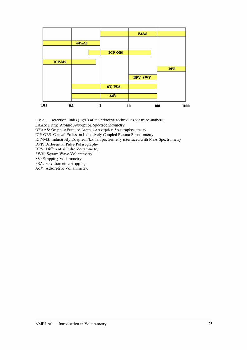
AMEL srl – Introduction to Voltammetry 25
Fig 21 – Detection limits (µg/L) of the principal techniques for trace analysis.
FAAS: Flame Atomic Absorption Spectrophotometry
GFAAS: Graphite Furnace Atomic Absorption Spectrophotometry
ICP-OES: Optical Emission Inductively Coupled Plasma Spectrometry
ICP-MS: Inductively Coupled Plasma Spectrometry interfaced with Mass Spectrometry
DPP: Differential Pulse Polarography
DPV: Differential Pulse Voltammetry
SWV: Square Wave Voltammetry
SV: Stripping Voltammetry
PSA: Potentiometric stripping
AdV: Adsorptive Voltammetry.
AMEL srl – Introduction to Voltammetry 26
7. QUALITATIVE ANALYSIS
Voltammetry is not dedicated to the quantitative analysis. In fact the peak
potential or the half wave potential can vary depending on the sample matrix, the
type of supporting electrolyte and on the presence of chelating reagents. When
necessary the presence/absence of an analyte is proved by the enrichment technique,
namely, by adding an aliquot of standard solution.
8. QUANTITATIVE ANALYSIS
The peak (or wave) height is proportional to the concentration of the analyte,
as it is shown in table 4.
Quantitative analysis is than performed considering the peak (or wave) height
and using the (single or multiple) standard addition method. This is in fact the best
method for lowering the matrix interference. When the sample matrix is very simple
or reproducible the calibration curve methods could be used.
8.1 – Standard addition method
The unknown concentration of a sample can be established with usual
quantitative methods if only some kind of interference don’t take place • During the titration, for example, the titrant has to react exclusively with the
analyte. If one or more substances that could react with the analyte are present in
the sample matrix, this interference has to be removed or, at least, neutralised.
• If an analyst prepare a calibration curve using standard solution in distilled water,
some difficulties could be encountered if the sample to be analysed has a complex
matrix (meaning a matrix rich of general chemical compounds). In fact, these
substances can vary significantly some physical characteristics of the solution,
(like viscosity, or refraction index and so on), or they can vary the not specific
background instrumental signal or the analyte signal, or, finally, they could
increase or decrease the analytical signal, reacting with the analyte or with the
specifying reagent added to the solution in order to give rise to the instrumental
signal. Also in this case, attempts have to be made to remove or neutralise the
effect of the interfering substances, or instead, to prepare standard solutions in a
matrix similar to the sample one. Anyway, whatever the analytical method is used, the interference affects are to be removed, avoiding analytical errors. The best method to avoid some matrix interference is the multiple standard addition method or, simpler, the single standard addition method. These methods, unfortunately, cannot allow to compensate the not specific interference that raise the background signal. The only valid strategy to compensate this kind of interference is to measure the signal as difference between the analytical signal and a background of a blank solution, or, at least, to zero the signal with an appropriate blank solution. Essential condition for the use of the standard addition in Voltammetry is to
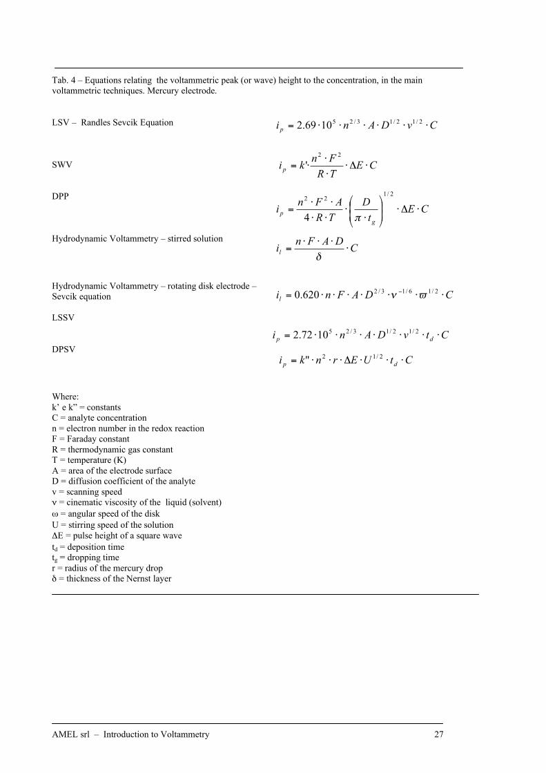
make the scanning related to each addition using the same parameters. In table 4 are
reported the equations correlating the concentration to the peak (or wave) height for
the most important voltammetric techniques. As can be seen, several are the
parameters to be considered in order to keep constant the proportionality between
concentration and peak (or wave) height among different scanning.
Another important condition is to work in the linear range of the relation
between concentration and peak (or wave) height. This range, in some case is very
narrow.
AMEL srl – Introduction to Voltammetry 27
Tab. 4 – Equations relating the voltammetric peak (or wave) height to the concentration, in the main
voltammetric techniques. Mercury electrode.
LSV – Randles Sevcik Equation
SWV
DPP
Hydrodynamic Voltammetry – stirred solution
Hydrodynamic Voltammetry – rotating disk electrode –
Sevcik equation
LSSV
DPSV
Where:
k’ e k” = constants
C = analyte concentration
n = electron number in the redox reaction
F = Faraday constant
R = thermodynamic gas constant
T = temperature (K)
A = area of the electrode surface
D = diffusion coefficient of the analyte
v = scanning speed
! = cinematic viscosity of the liquid (solvent)
" = angular speed of the disk
U = stirring speed of the solution
#E = pulse height of a square wave
td = deposition time
tg = dropping time
r = radius of the mercury drop
$ = thickness of the Nernst layer
CvDAnip !!!!!!=2/12/13/25
1069.2
CETR
Fnkip !"!
!
!!=
22
'
CEt
D
TR
AFni
g
p !"!##
$
%
&&
'
(
!!
!!
!!=
2/122
4 )
CDAFn
il
!!!!
="
CDAFnil
!!!!!!!=" 2/16/13/2
620.0 #$
CtvDAni dp !!!!!!!=2/12/13/25
1072.2
CtUErnki dp !!!"!!!=2/12
"
AMEL srl – Introduction to Voltammetry 28
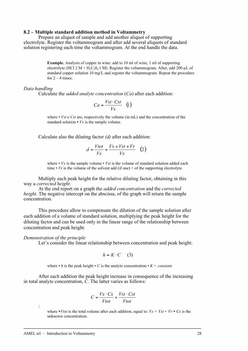
8.2 – Multiple standard addition method in Voltammetry Prepare an aliquot of sample and add another aliquot of supporting electrolyte. Register the voltammogram and after add several aliquots of standard solution registering each time the voltammogram. At the end handle the data.
Example. Analysis of copper in wine: add to 10 ml of wine, 1 ml of supporting
electrolyte (HCl 2 M + H2C204 1 M). Register the voltammogram. After, add 200 µL of
standard copper solution 10 mg/L and register the voltammogram. Repeat the procedure
for 2 – 4 times.
Data handling Calculate the added analyte concentration (Ca) after each addition:
where • Vst e Cst are, respectively the volume (in mL) and the concentration of the
standard solution • Vx is the sample volume.
Calculate also the diluting factor (d) after each addition:
where • Vx is the sample volume • Vst is the volume of standard solution added each
time • Vr is the volume of the solvent add (if one) + of the supporting electrolyte.
Multiply each peak height for the relative diluting factor, obtaining in this way a corrected height. At the end report on a graph the added concentration and the corrected height. The negative intercept on the abscissa, of the graph will return the sample concentration.
This procedure allow to compensate the dilution of the sample solution after
each addition of a volume of standard solution, multiplying the peak height for the
diluting factor and can be used only in the linear range of the relationship between
concentration and peak height. Demonstration of the principle Let’s consider the linear relationship between concentration and peak height:
where • h is the peak height • C is the analyte concentration • K = constant.
After each addition the peak height increase in consequence of the increasing in total analyte concentration, C. The latter varies as follows:
: where !Vtot is the total volume after each addition, equal to: Vx + Vst + Vr ! Cx is the
unknown concentration.
( )1Vx
CstVstCa
!=
( )2Vx
VrVstVx
Vx
Vtotd
++==
)3(CKh !=
Vtot
CstVst
Vtot
CxVxC
!+
!=
AMEL srl – Introduction to Voltammetry 29
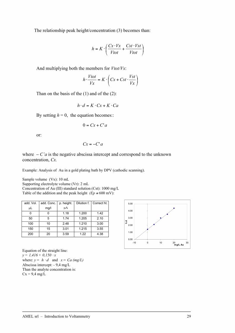
The relationship peak height/concentration (3) becomes than:
And multiplying both the members for Vtot/Vx:
Than on the basis of the (1) and of the (2):
By setting h = 0, the equation becomes::
or:
where – C’a is the negative abscissa intercept and correspond to the unknown
concentration, Cx.
Example: Analysis of Au in a gold plating bath by DPV (cathodic scanning).
Sample volume (Vx): 10 mL
Supporting electrolyte volume (Vr): 2 mL
Concentration of Au (III) standard solution (Cst): 1000 mg/L
Table of the addition and the peak height (Ep ! 600 mV):
add. Vol. add. Conc. p. height. Dilution f. Correct ht.
µL mg/l µ%
0 0 1.18 1.200 1.42
50 5 1.74 1.205 2.10
100 10 2.48 1.210 3.00
150 15 3.01 1.215 3.55
200 20 3.59 1.22 4.38
Equation of the straight line:
y = 1,416 + 0,150 " x
where: y = h " d and x = Ca (mg/L)
Abscissa intercept: - 9,4 mg/L
Than the analyte concentration is:
Cx = 9,4 mg/L
!"
#$%
& '+
''=
Vtot
VstCst
Vtot
VxCxKh
!"
#$%
&'+'='Vx
VstCstCxK
Vx
Vtoth
CaKCxKdh !+!=!
aCCx '0 +=
aCCx '!=
0.00
1.00
2.00
3.00
4.00
5.00
-10 0 10 20 30mg/L Au
h.d
AMEL srl – Introduction to Voltammetry 30
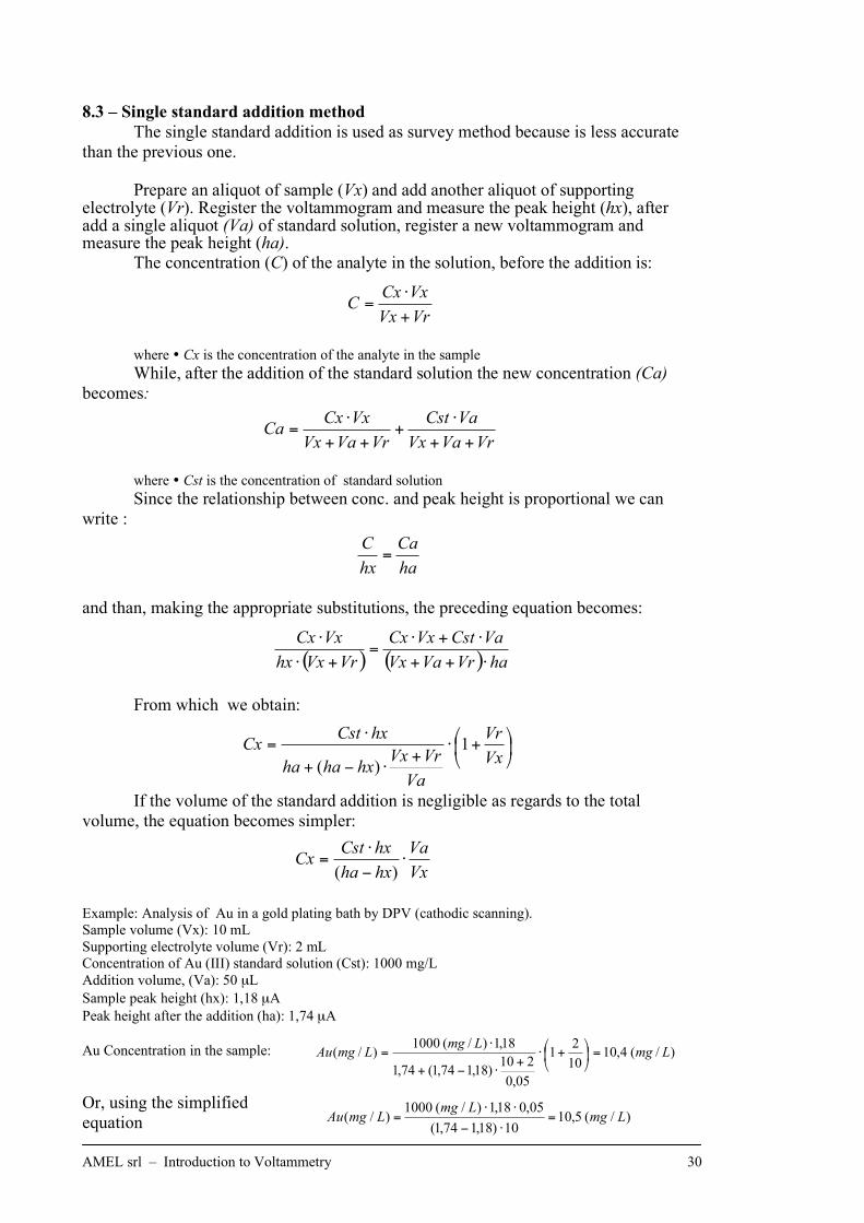
8.3 – Single standard addition method
The single standard addition is used as survey method because is less accurate
than the previous one.
Prepare an aliquot of sample (Vx) and add another aliquot of supporting electrolyte (Vr). Register the voltammogram and measure the peak height (hx), after add a single aliquot (Va) of standard solution, register a new voltammogram and measure the peak height (ha).
The concentration (C) of the analyte in the solution, before the addition is:
where ! Cx is the concentration of the analyte in the sample
While, after the addition of the standard solution the new concentration (Ca)
becomes:
where ! Cst is the concentration of standard solution Since the relationship between conc. and peak height is proportional we can
write :
and than, making the appropriate substitutions, the preceding equation becomes:
From which we obtain:
If the volume of the standard addition is negligible as regards to the total
volume, the equation becomes simpler:
Example: Analysis of Au in a gold plating bath by DPV (cathodic scanning).
Sample volume (Vx): 10 mL
Supporting electrolyte volume (Vr): 2 mL
Concentration of Au (III) standard solution (Cst): 1000 mg/L
Addition volume, (Va): 50 µL
Sample peak height (hx): 1,18 µA
Peak height after the addition (ha): 1,74 µA
Au Concentration in the sample:
Or, using the simplified
equation
VrVx
VxCxC
+
!=
VrVaVx
VaCst
VrVaVx
VxCxCa
++
!+
++
!=
ha
Ca
hx
C=
( ) ( ) haVrVaVx
VaCstVxCx
VrVxhx
VxCx
!++
!+!=
+!
!
!"
#$%
&+'
+'(+
'=
Vx
Vr
Va
VrVxhxhaha
hxCstCx 1
)(
Vx
Va
hxha
hxCstCx !
"
!=
)(
)/(4,1010
21
05,0
210)18,174,1(74,1
18,1)/(1000)/( Lmg
LmgLmgAu =!
"
#$%
&+'
+'(+
'=
)/(5,1010)18,174,1(
05,018,1)/(1000)/( Lmg
LmgLmgAu =
!"
!!=
AMEL srl – Introduction to Voltammetry 31
9. STEPS IN A VOLTAMMETRIC ANALYSIS
Sample treatment
For a voltammetric analysis the sample has to be a solution. If the sample is
solid, it has to be dissolved in a proper way. Liquids with complex matrix and low
soluble solids are to be digested or extracted. Rarely, it is not necessary to digest
complex matrices, i.e. the analysis of ascorbic acid in fruit juice can be performed
without any treatment.
At the end of any treatment the obtained solution has to have the following
characteristics:
- No suspended solids. If present they have to be eliminated by filtering or
centrifuging. The separate solid can be analysed separately.
- No colloids. Colloids compete with electrochemical processes, sometime
stopping them or keeping them not reproducible. Often a simple oxidising
treatment with UV lamp is sufficient to overcome this interference.
- No surfactants, because they also can stop the electrochemical processes
or decreasing the sensitivity of the method. Also in this case a simple
oxidising treatment with UV lamp is sufficient to overcome this
interference.
- pH between 1 and 10 (also 12 in NaOH is not present) and atmosphere
neither too much oxidising nor too much reducing, otherwise the mercury
electrode can react or give raise to a very noisy signal. This latter
phenomena effect also solids electrode. Digested solutions have to be
accurately neutralised or buffered. It is necessary also to boil the digested
solution until the nitrous or hydrogen peroxide not react or other vapours
are removed from solution.
- If the analysis is performed in a solvent different from water, when
possible, an electrolyte has to be added increasing the electrical
conductivity of the solution
Addition of the supporting electrolyte
Every analysis has to be performed using a typical supporting electrolyte. The characteristics of this
solution is described in the manual or reported in literature.
Bubbling of the solution with nitrogen
Oxygen is always present in solution and give rise to 2 voltammetric peaks; the first at 0 V and the
other one at 1 V. This gas has to be eliminated from the solution before the analysis, by a prolonged
bubbling of nitrogen. Lower is the analyte concentration to be found, greater has to be the bubbling
time.
Pause (delay)
Solution has to be leave quiescent stopping after the bubbling.
Electrode cleaning
- Mercury electrode: some drops are discharged
- Solid electrode: an inverse scanning has to be performed
Scanning and registration of the sample voltammogram
Addition of standard solution of analyte
AMEL srl – Introduction to Voltammetry 32
Scanning and registration of the voltammogram after the addition (the process is repeated 2-
8times)
Measure of the all peak (or wave) heights
Drawing the graph
Reading of the unknown concentration
10. TRACE ANALYSIS OF METALS
10.1 – Cleaning procedure for glassware and working area
Trace analysis need sophisticated and very sensitive instruments. Results
cannot reach the same reproducibility as for high concentration analysis. In fact,
typical percentages of standard deviation of results in trace analysis are in the range
of 15-20%.
Moreover, lead, zinc, iron and sodium are environmental pollutants. These
metals are very widespread and it is very difficult to find any material completely
lacking in these metals. Distilled and deionized water, acids and chemicals normally
used for the preparation of solutions or for the sample treatment are anyway polluted
with these metals. A also in the air powder is polluted and some time some particle
of pollutants can fall down in sample or standard solutions, before or during the
analysis.
For these reasons is mandatory to adopt strict cleaning procedure, especially
for the analysis of lead, zinc, iron and sodium. The best strategy to avoid errors
consist in:
- the cleaning of the glassware for the analysis,
- the analysis of the blank solutions
- the control of the analytical data.
Finally, the analysis of mercury has to be performed with dedicated glassware
to avoid any pollution. (don’t use the same glassware used for the analysis with
mercury drop or film electrode). Stock gold electrode and cells far from mercury and
accurately clean Pt and reference electrodes, magnetic rod and the top of the cell.
Obviously analyse Pt using a glassy carbon reference electrode (instead a Pt one… )
10.2 – Glassware cleaning
Stock the glassware (volumetric flasks, pipette and bottles) dedicated to the
preparation of standard solutions far from the one for the sample treatments.
Clean the glassware with copious distilled water, then with 1-2% HNO3 and
finally, again with copious distilled water.
Dip the cells in 1-5% HNO3 at the end of the analysis till a new analytical
session. Don’t use the same cell for the following analysis.
Accurately clean the instrument and the working area (pay attention to the
powder falling down from old fume hood….)
Copiously wash the electrodes and the top of the cell at the end of the
analysis.
Preferably start with low concentration sample analysis and continue with
high concentration ones.
AMEL srl – Introduction to Voltammetry 33
11. MAINTENANCE AND CLEANING
11.1 - Mercury drop electrode
- At the end of each analysis, wash the capillary with distilled water; take care to
avoid to aim the water flow directly on the tip of the capillary. Clean while the
mercury valve (function n. 6 of the supporting block: Start to open mercury
valve). Pay attention to avoid the water flows into the capillary and to avoid the
scattering of mercury drops on the working area.
- At the end of a working day, accurately wash the capillary, dry it and leave the
capillary with a drop dropping from the tip (use function n. 6 of the supporting
block: Start to open mercury valve) in a clean and dry cell. Check that there are
not salt deposits nearby the tip of the capillary.
- During long periods of inactivity it is better to make a scanning with an
indifferent supporting electrolyte (i.e. 0.1 M KCl) every week (or two) avoiding
the stagnation of mercury in the capillary.
- If the capillary is obstructed , or if the current don’t flow in the circuit, or if the
noise of the signal is very high, try to set it free applying the vacuum pump at the
end of the capillary. When the maximum of the vacuum is reached, open the
mercury valve (use function n. 6 of the supporting block: Start to open mercury
valve). Aspirate some mercury drop and disconnect the tube of the vacuum pump
(remember: don’t close the water tap before disconnecting the tube). If the
problem cannot to be solved, change the capillary.
- Stock the exhausted mercury in a strictly closed polythene bottles, under a
water layer. Don’t leave the bottle open !
- Mercury waste can occur during the maintenance procedure or during the
replacement of the capillary. Due to the mercury toxicity and vapour pressure the
scattered drops must be recovered using a vacuum pump and the working area
must be cleaned using proper devices (cleaning kits are available).
11.2 - Gold, platinum and glassy carbon electrodes
Main sources of surface pollution for solid electrodes are fat (or hydrophobic
compounds), arising typically from the fingers of the operator. Clean solid electrodes
carefully rubbing the active surface with soft paper imbibed with acetone or thin
abrasive paste (i.e. 0.3 µ alumina powder in distilled water). Rinse finally with
distilled water and check that the electrode surface is mirrored using a lens.
Deep incrusted electrodes in 2 M HNO3 and rinse with distilled water.
After the cleaning and, anyway, every time a new electrode is used, make a
cathodic cleaning at a potential which can discharge any metallic impurity. It’s better
to make the cathodic cleaning also before each potential scanning, during an
analysis.
Store clean and dry electrodes at the air, without any further particular care.
Quality of the electrode surface can be controlled analysing a blank or a
reference solution.
11.3 - Auxiliary platinum electrode
The auxiliary platinum electrode has to be cleaned and stored just like the
other solid electrodes. The cathodic cleaning is no necessary.
11.4 - Reference electrode
Reference electrode contains a concentrated solution of a salt (normally KCl)
which ions have the same mobility to diminish the junction. Those solution is, of
AMEL srl – Introduction to Voltammetry 34
course, saturated of AgCl. During analysis is mandatory to check that the ions of the
sample don’t interfere with the ones present in the internal reference electrode
solution. It could happen in the following situations:
analysis of traces of silver
analysis of chloride
analysis of sulphide, bromide and iodide that can react with Ag developing
insoluble salts and obstructing the diaphragm and, at the end, increasing the junction
potential.
These problems can be overcome using a double junction reference electrode,
containing a KNO3 solution as a final junction.
Moreover the level of the internal solution of the reference electrode has to be
higher than the level of the external sample solution in the cell assuring a very low
flow of solution from the inner toward the outer (and not vice and versa). In this way
the pollution of the internal solution of the reference electrode is reduced and the
potential readings are more reproducible.
When a diaphragm is obstructed (that means that the peak position fluctuate
among different scanning) it is better to change completely the glassy body of the
electrode.
After periods of inactivity the electrode cover itself by a white layer of KCl.
Simply wash the electrode with distilled water and if necessary add more 3 M KCl
internal solution.
11.5 - Cells
Clean glass and Teflon cells using distilled water or acid solution.
Dip the cells in 5 – 10% HNO3 for 2 –3 days before the trace analyse of
metals.
12. PREPARING FILM ELECTRODES
12.1 - Mercury film on glassy carbon electrode
- Dip the clean glassy carbon electrode in a 800 mg/l in 1.3 M HC1 Hg2+
solution, or
in a 1000 mg/l Hg2+
solution for AA Spectrophotometry
- Bring the electrode potential at -1100 mV for 2 minutes
- Rinse with distilled water.
- Never leave the electrode to dry
- Don’t touch the Hg film for any reason film
- Check if the surface of the film is uniform, grey and opaque before the use. If not,
clean the electrode using soft paper, rinse with water and depose another film.
- Store the Hg film electrode in distilled water until next analysis. Before starting a
new series of analysis, check the electrode performances (see KCl test).
- After the first time it is necessary to run a series of scanning before the electrode
rise to a complete settlement.
Maintenance and cleaning of mercury film electrode on glassy carbon
Store the mercury film electrode dipped in distilled water. When in use, leave
it on air only for short periods.
When the film is clearly scratched or striped, clean it with soft paper, rinse
with distilled water and depose e new film.
AMEL srl – Introduction to Voltammetry 35
12.2 - Gold film electrode on glassy carbon
- Dip the clean glassy carbon electrode in a Au3+
solution (1000 mg/l in 1 M HC1)
- Bring the electrode potential at -400 mV for 2 minutes i.
- Rinse with distilled water.
- Never leave the electrode to dry
- Don’t touch the Au film for any reason film
- Check if the surface of the film is uniform, gilded before the use. If not, clean the
electrode using soft paper, rinse with water and depose another film.
- Store the Au film electrode in distilled water until next analysis. Before starting a
new series of analysis, check the electrode performances.
Maintenance e cleaning of gold film electrode
Store the gold film electrode dipped in distilled water. When in use, leave it
on air only for short periods.
When the film is clearly scratched or striped, clean it with very thin abrasive
paste on soft paper, rinse with distilled water and depose e new film.
13. REAGENTS FOR TRACE ANALYSIS
Use only reagents for trace analysis grade. If this is not possible analyse blank
solution before sample analysis.
13.1 – Preparing standard solutions
Buy directly the concentrated standard solution of metals (1 g/l of the
analyte). The solution for AAS are generally suitable.
Prepare standard solutions anions or organic compounds starting from a pure,
analytical grade substance. Dry the substance in a oven at 110°C eliminating the
humidity if this procedure do not compromise the stability of the compound.
Prepare diluted standard solutions starting from the concentrated ones. Add 1-
2% HNO3 unless it is differently specified.
Throw away the standard solutions less than 100 mg/l at the end of an
analytical session.
13.2 – Preparing supporting electrolytes
Prepare supporting electrolytes using pure, analytical grade reagents. It’s
better to check the presence of the analyte in the blank, before starting the analysis.
The most common supporting electrolyte and buffer are the following:
0.1 M EDTA solution
Dissolve 37.2 g of EDTA-Na2 in 1 l of distilled water, in a volumetric flask.
0.1 or 1 M HCl solution
Dilute 8.2 (or 82) ml of 37% HCl in 1 l of distilled water, in a volumetric flask.
0.1 or 1 M KCl solution
Dissolve 7.5 (o 75) g of KCl in 1 l of distilled water, in a volumetric flask.
0.1 M KCNS solution
Dissolve 9.72 g of KCNS in 1 l of distilled water, in a volumetric flask.
AMEL srl – Introduction to Voltammetry 36
0.1 o 1 M KNO3 solution
Dissolve 10 (o 100) g of KNO3 in 1 l of distilled water, in a volumetric flask.
0.1 M LiCl / LiOH solution
Dissolve 2.4 g of LiOH and 4.3 g of LiCl in 1 l of distilled water, in a volumetric
flask.
1 M NaF solution
Dissolve 42 g of NaF in 1 l of distilled water, in a volumetric flask. Heat if
necessary.
0.1 M acetate buffer solution at pH 4.5 (CH3COONa / CH3COOH)
Dissolve 8.2 g of anhydrous CH3COONa (or 13.6 g of CH3COONa&3H2O) in 800 ml
of distilled water. Add 5.75 ml of glacial CH3COOH. Check the pH. Bring to mark
volume in a 1 l volumetric flask with distilled water.
0.1 M ammonia buffer solution at pH 9.4 (NH4Cl / NH3)
Dissolve 5.4 g of NH4Cl in 900 ml of water. Add 6.9 ml of 26% NH3. Check the pH.
Bring to mark in a 1 l volumetric flask with distilled water.
0.1 M borate buffer solution at pH 9.5 (NaH2BO3 / H3BO3)
Dissolve 5.1 g of H3BO3 in 900 ml of water. Add 2 g of NaOH. Check the pH. Bring
to mark in a 1 l volumetric flask with distilled water.
Britton Robinson buffer solution at various pH
Common solution
Mix:
- 100 ml of 0.04 M H3BO3 (2.04 g / 100 ml) aqueous solution.
- 100 ml of 0.04 M CH3COOH (2.3 ml of glacial CH3COOH / 100 ml) aqueous
solution.
- 100 ml of 0.04 M H3PO4 ( 2.8 ml of 85% H3PO4 / 100 ml) aqueous solution.
Solutions at desired pH:
Bring the preceding solution at the desired pH Using a 0.2 M NaOH solution.
0.2 M ammonia citrate buffer solution at pH 3 (ammonia citrate / citric acid)
Dissolve 42.5 g of mono hydrate citric acid in 800 ml of water. Add 26% NH3 until
pH 3. Bring to mark in a 1 l volumetric flask with distilled water.
0.2 M sodium citrate buffer solution at pH 3 (sodium citrate / citric acid)
Dissolve 42.5 g of mono hydrate sodium citrate in 800 ml of water. Add 20% NaOH
until pH 3. Bring to mark in a 1 l volumetric flask with distilled water.
0.2 M phosphate buffer solution at pH 6.8
Dissolve 24 g of NaH2PO4&H2O in 800 ml of water. Add 85% H3PO4 until pH 6.8.
Bring to mark in a 1 l volumetric flask with distilled water.
0.2 M ammonia tartrate buffer solution at pH 9 (ammonia tartrate / tartaric acid)
Dissolve 300 g of tartaric acid in 800 ml of water. Add 26% NH3 until pH 9. Bring to
mark in a 1 l volumetric flask with distilled water.
AMEL srl – Introduction to Voltammetry 37
0.2 M sodium tartrate buffer solution at pH 9 (sodium tartrate / tartaric acid)
Dissolve 300 g of tartaric acid in 800 ml of water. Add 20% NaOH until pH 9. Bring
to mark in a 1 l volumetric flask with distilled water.
0.3 M TEA / 0.1 M KOH buffer solution
Dissolve 45 g of TEA (triethanolamine) and 5.6 g of KOH in 1 l of distilled water, in
a volumetric flask.
0.3 M TEA / 0.1 M NaOH buffer solution
Dissolve 45 g of TEA (triethanolamine) and 8 g of NaOH in 1 l of distilled water, in
a volumetric flask.
14. CHECKING THE POLAROGRAPH PERFORMANCES
14.1 - 0.1 M KCl test
The following test allows to check if the instrument (particularly the
capillary) works correctly and maintains the his performances for a long the time.
Activate this procedure immediately, just before the instrument reach your
laboratory, collecting in this way an “historical” data series as reference.
Reagents
- 10 mg/l Cadmium standard solution. Prepare a fresh solution before each analysis,
starting from a 1000 mg/l standard solution.
- 0.1 M KCl checking solution. Dissolve 15 g of KCl in 2 litres of 1% HNO3 (20 ml
of 65% HNO3 in 2 l of distilled water), in a volumetric flask, add 100 µl of Cd
standard solution (1 g/l). Store this solution in a polythene bottle. Use the same solid
KCl, stored in a polythene bottle, if prolonged check are needed.
Procedure
Every time an analytical series start (it means each day, or week…) pour 10 ml of
checking solution in the cell. Bubble nitrogen for 5 minutes. Analyse Cadmium using
single (quicker) or multiple (longer) standard addition (100 µl of 10 mg/1 Cd each
addition).
Prepare a control chart after 10 – 15 analysis,.
Results control
- The peak position has to be constant, into a specific confidential range. Use
statistics and control chart for this purpose.
If the peak position significantly varies check the conditions of the reference
electrode
- During the time, the results of the analysis have to agree to each other, into a
confidential range. Use statistics and control chart for this purpose.
If the results do not agree to each other verify the following:
- quality of the solutions (KCl and Cd standard solutions)
- the conditions of the capillary
- the cleaning procedure for the glassware, the instrument and the operator
Warning ! Strong smokers have the finger dirty of high level of Cadmium. If
necessary, change the analyte of the checking procedure (avoid anyway lead,
iron and zinc because they are environmental pollutant anyway !)


