John von Neumann Institute for Computing

Introduction to Molecular Dynamics Simulation

Michael P. Allen

published in

Computational Soft Matter: From Synthetic Polymers to Proteins,Lecture Notes,Norbert Attig, Kurt Binder, Helmut Grubmuller, Kurt Kremer (Eds.),John von Neumann Institute for Computing, Julich,NIC Series, Vol. 23, ISBN 3-00-012641-4, pp. 1-28, 2004.

c© 2004 by John von Neumann Institute for ComputingPermission to make digital or hard copies of portions of this workfor personal or classroom use is granted provided that the copiesare not made or distributed for profit or commercial advantage andthat copies bear this notice and the full citation on the first page. Tocopy otherwise requires prior specific permission by the publishermentioned above.

http://www.fz-juelich.de/nic-series/volume23

Introduction to Molecular Dynamics Simulation

Michael P. Allen

Centre for Scientific Computing and Department of Physics,University of Warwick, Coventry CV4 7AL, United Kingdom

E-mail: m.p.allen@warwick.ac.uk

In this chapter a summary is given of the key ingredients necessary to carry out a molecular

dynamics simulation, with particular emphasis on macromolecular systems. We discuss the

form of the intermolecular potential for molecules composed of atoms, and of non-spherical

sub-units, giving examples of how to compute the forces and torques. We also describe some

of the MD algorithms in current use. Finally, we briefly refer to the factors that influence the

size of systems, and length of runs, that are needed to calculate statistical properties.

1 The Aims of Molecular Dynamics

We carry out computer simulations in the hope of understanding the properties of assem-

blies of molecules in terms of their structure and the microscopic interactions between

them. This serves as a complement to conventional experiments, enabling us to learn

something new, something that cannot be found out in other ways. The two main families

of simulation technique are molecular dynamics (MD) and Monte Carlo (MC); addition-

ally, there is a whole range of hybrid techniques which combine features from both. In

this lecture we shall concentrate on MD. The obvious advantage of MD over MC is that it

gives a route to dynamical properties of the system: transport coefficients, time-dependent

responses to perturbations, rheological properties and spectra.

Computer simulations act as a bridge (see Fig. 1) between microscopic length and time

scales and the macroscopic world of the laboratory: we provide a guess at the interactions

between molecules, and obtain ‘exact’ predictions of bulk properties. The predictions are

‘exact’ in the sense that they can be made as accurate as we like, subject to the limita-

tions imposed by our computer budget. At the same time, the hidden detail behind bulk

measurements can be revealed. An example is the link between the diffusion coefficient

and velocity autocorrelation function (the former easy to measure experimentally, the latter

much harder). Simulations act as a bridge in another sense: between theory and experi-

ment. We may test a theory by conducting a simulation using the same model. We may

test the model by comparing with experimental results. We may also carry out simulations

on the computer that are difficult or impossible in the laboratory (for example, working at

extremes of temperature or pressure).

Ultimately we may want to make direct comparisons with experimental measurements

made on specific materials, in which case a good model of molecular interactions is essen-

tial. The aim of so-called ab initio molecular dynamics is to reduce the amount of fitting

and guesswork in this process to a minimum. On the other hand, we may be interested

in phenomena of a rather generic nature, or we may simply want to discriminate between

good and bad theories. When it comes to aims of this kind, it is not necessary to have a

perfectly realistic molecular model; one that contains the essential physics may be quite

suitable.

1

IntermolecularT

r

t

c(t)

P

Structure

Dynamics

Phasess

lg

g(r)

r

v(r)

potentialComplex Fluid(real system)

Complex Fluid

(model system)

Make modelSimulation

ExperimentalResults

Results

PredictionsTheoretical

Test theory

Test model

Figure 1. Simulations as a bridge between (a) microscopic and macroscopic; (b) theory and experiment.

2 Molecular Interactions

Molecular dynamics simulation consists of the numerical, step-by-step, solution of the

classical equations of motion, which for a simple atomic system may be written

miri = f i f i = − ∂

∂riU (1)

For this purpose we need to be able to calculate the forces f i acting on the atoms, and these

are usually derived from a potential energy U(rN ), where rN = (r1, r2, . . .rN ) repre-

sents the complete set of 3N atomic coordinates. In this section we focus on this function

U(rN ), restricting ourselves to an atomic description for simplicity. (In simulating soft

condensed matter systems, we sometimes wish to consider non-spherical rigid units which

have rotational degrees of freedom: rotational equations of motion and interaction poten-

tials will be considered in section 5).

2.1 Non-bonded Interactions

The part of the potential energy Unon-bonded representing non-bonded interactions between

atoms is traditionally split into 1-body, 2-body, 3-body . . . terms:

Unon-bonded(rN ) =

∑i

u(ri) +∑

i

∑j>i

v(ri, rj) + . . . . (2)

The u(r) term represents an externally applied potential field or the effects of the container

walls; it is usually dropped for fully periodic simulations of bulk systems. Also, it is

usual to concentrate on the pair potential v(ri, rj) = v(rij) and neglect three-body (and

higher order) interactions. There is an extensive literature on the way these potentials are

determined experimentally, or modelled theoretically1–4.

In some simulations of complex fluids, it is sufficient to use the simplest models that

faithfully represent the essential physics. In this chapter we shall concentrate on continu-

ous, differentiable pair-potentials (although discontinuous potentials such as hard spheres

2

0 0.5 1 1.5 2 2.5 3r / σ

-2

-1

0

1

2

3

4

v / ε

Lennard-Jones

-4r-6

4r-12

WCA

Figure 2. Lennard-Jones pair potential showing the r−12 and r−6 contributions. Also shown is the WCA shifted

repulsive part of the potential.

and spheroids have also played a role, see e.g. 5). The Lennard-Jones potential is the most

commonly used form:

vLJ(r) = 4ε

[(σ

r

)12

−(σ

r

)6]

. (3)

with two parameters: σ, the diameter, and ε, the well depth. This potential was used,

for instance, in the earliest studies of the properties of liquid argon6, 7 and is illustrated

in Fig. 2. For applications in which attractive interactions are of less concern than the

excluded volume effects which dictate molecular packing, the potential may be truncated

at the position of its minimum, and shifted upwards to give what is usually termed the WCA

model8. If electrostatic charges are present, we add the appropriate Coulomb potentials

vCoulomb(r) =Q1Q2

4πε0r, (4)

where Q1, Q2 are the charges and ε0 is the permittivity of free space. The correct handling

of long-range forces in a simulation is an essential aspect of polyelectrolyte simulations,

which will be the subject of the later chapter of Holm9.

2.2 Bonding Potentials

For molecular systems, we simply build the molecules out of site-site potentials of the form

of Eq. (3) or similar. Typically, a single-molecule quantum-chemical calculation may be

used to estimate the electron density throughout the molecule, which may then be mod-

elled by a distribution of partial charges via Eq. (4), or more accurately by a distribution of

electrostatic multipoles4, 10. For molecules we must also consider the intramolecular bond-

ing interactions. The simplest molecular model will include terms of the following kind:

3

1

3

φ 1234

234

4

2

θ23r

Figure 3. Geometry of a simple chain molecule, illustrating the definition of interatomic distance r23, bend angle

θ234, and torsion angle φ1234.

Uintramolecular =1

2

∑bonds

krij

(rij − req

)2(5a)

+1

2

∑bend

angles

kθijk

(θijk − θeq

)2(5b)

+1

2

∑torsionangles

∑m

kφ, mijkl

(1 + cos(mφijkl − γm)

)(5c)

The geometry is illustrated in Fig. 3. The “bonds” will typically involve the separation

rij = |ri −rj | between adjacent pairs of atoms in a molecular framework, and we assume

in Eq. (5a) a harmonic form with specified equilibrium separation, although this is not

the only possibility. The “bend angles” θijk are between successive bond vectors such as

ri − rj and rj − rk, and therefore involve three atom coordinates:

cos θijk = rij · rjk =(rij · rij

)−1/2(rjk · rjk

)−1/2(rij · rjk

)where r = r/r. Usually this bending term is taken to be quadratic in the angular dis-

placement from the equilibrium value, as in Eq. (5b), although periodic functions are also

used. The “torsion angles” φijkl are defined in terms of three connected bonds, hence four

atomic coordinates:

cos φijkl = −nijk · njkl , where nijk = rij × rjk , njkl = rjk × rkl ,

and n = n/n, the unit normal to the plane defined by each pair of bonds. Usually the

torsional potential involves an expansion in periodic functions of order m = 1, 2, . . .,Eq. (5c).

A simulation package force-field will specify the precise form of Eq. (5), and the var-

ious strength parameters k and other constants therein. Actually, Eq. (5) is a consider-

able oversimplification. Molecular mechanics force-fields, aimed at accurately predicting

4

structures and properties, will include many cross-terms (e.g. stretch-bend): MM311–13 and

MM414–16 are examples. Quantum mechanical calculations may give a guide to the “best”

molecular force-field; also comparison of simulation results with thermophysical proper-

ties and vibration frequencies is invaluable in force-field development and refinement. A

separate family of force fields, such as AMBER17, 18, CHARMM19 and OPLS20 are geared

more to larger molecules (proteins, polymers) in condensed phases; their functional form

is simpler, closer to that of Eq. (5), and their parameters are typically determined by quan-

tum chemical calculations combined with thermophysical and phase coexistence data. This

field is too broad to be reviewed here; several molecular modelling texts21–23 (albeit target-

ted at biological applications) should be consulted by the interested reader. The modelling

0 0.5 1 1.5

r / σ

0

50

100

150

200

v / ε

FENE+WCAFENEWCAharmonic

Figure 4. The FENE+WCA potential, with its separate FENE (attractive) and WCA (repulsive) components,

between bonded atoms in a coarse-grained polymer chain. Also shown is the equivalent harmonic potential.

Unlike the harmonic spring, the FENE potential cannot be extended beyond a specified limit, here R0 = 1.5σ.

For more details see Ref. 24.

of long chain molecules will be of particular interest to us, especially as an illustration of

the scope for progressively simplifying and “coarse-graining” the potential model. Var-

ious explicit-atom potentials have been devised for the n-alkanes25. More approximate

potentials have also been constructed26–28 in which the CH2 and CH3 units are represented

by single “united atoms”. These potentials are typically less accurate and less transfer-

able than the explicit-atom potentials, but significantly less expensive; comparisons have

been made between the two approaches29. For more complicated molecules this approach

may need to be modified. In the liquid crystal field, for instance, a compromise has been

suggested30: use the united-atom approach for hydrocarbon chains, but model phenyl ring

hydrogens explicitly.

In polymer simulations, there is frequently a need to economize further and coarse-

grain the interactions more dramatically: significant progress has been made in recent

years in approaching this problem systematically31, 32. Finally, the most fundamental prop-

erties, such as the entanglement length in a polymer melt33, may be investigated using a

5

simple chain of pseudo-atoms or beads (modelled using the WCA potential of Fig. 2, and

each representing several monomers), joined by an attractive finitely-extensible non-linear

elastic (FENE) potential24 which is illustrated in Fig. 4.

vFENE(r) =

−1

2kR20 ln

(1 − (r/R0)

2)

r < R0

∞ r ≥ R0

(6)

The key feature of this potential is that it cannot be extended beyond r = R0, ensuring (for

suitable choices of the parameters k and R0) that polymer chains cannot move through one

another.

2.3 Force Calculation

Having specified the potential energy function U(rN ), the next step is to calculate the

atomic forces

f i = − ∂

∂riU(rN )

For site-site potentials this is a simple exercise. For the intramolecular part of the potential,

it is a little more involved, but still a relatively straightforward application of the chain

rule. Examples of how to do it are given in appendix C of Ref. 34. As a simple illustration,

consider one of the bending potential terms for the polymer of Fig. 3, supposing that it may

be written

v = −k cos θ234 = −k(r23 · r23)−1/2(r34 · r34)

−1/2(r23 · r34)

This will contribute to the forces on all three atoms. To calculate these, we need:

∂

∂r2(r23 · r34) = r34

∂

∂r3(r23 · r34) = r23 − r34

∂

∂r4(r23 · r34) = −r23

∂

∂r2(r23 · r23) = 2r23

∂

∂r3(r23 · r23) = −2r23

∂

∂r4(r23 · r23) = 0

∂

∂r2(r34 · r34) = 0

∂

∂r3(r34 · r34) = 2r34

∂

∂r4(r34 · r34) = −2r34

and hence

∂

∂r2cos θ234 = r−1

23 r−134

(r34 −

r23 · r34

r223

r23

)∂

∂r3cos θ234 = r−1

23 r−134

(r23 · r34

r223

r23 −r23 · r34

r234

r34 + r23 − r34

)∂

∂r4cos θ234 = r−1

23 r−134

(r23 · r34

r234

r34 − r23

)

A similar approach applied to the torsional potential gives the forces on all four involved

atoms.

6

3 The MD Algorithm

Solving Newton’s equations of motion does not immediately suggest activity at the cutting

edge of research. The molecular dynamics algorithm in most common use today may even

have been known to Newton35. Nonetheless, the last decade has seen a rapid develop-

ment in our understanding of numerical algorithms; a forthcoming review36 and a book37

summarize the present state of the field.

Continuing to discuss, for simplicity, a system composed of atoms with coordinates

rN = (r1, r2, . . .rN ) and potential energy U(rN ), we introduce the atomic momenta

pN = (p1, p2, . . .pN ), in terms of which the kinetic energy may be written K(pN ) =∑Ni=1

∣∣pi

∣∣2/2mi. Then the energy, or hamiltonian, may be written as a sum of kinetic and

potential terms H = K + U . Write the classical equations of motion as

ri = pi/mi and pi = f i (7)

This is a system of coupled ordinary differential equations. Many methods exist to perform

step-by-step numerical integration of them. Characteristics of these equations are: (a) they

are ‘stiff’, i.e. there may be short and long timescales, and the algorithm must cope with

both; (b) calculating the forces is expensive, typically involving a sum over pairs of atoms,

and should be performed as infrequently as possible. Also we must bear in mind that the

advancement of the coordinates fulfils two functions: (i) accurate calculation of dynamical

properties, especially over times as long as typical correlation times τa of properties a of

interest (we shall define this later); (ii) accurately staying on the constant-energy hypersur-

face, for much longer times τrun τa, in order to sample the correct ensemble.

To ensure rapid sampling of phase space, we wish to make the timestep as large as

possible consistent with these requirements. For these reasons, simulation algorithms have

tended to be of low order (i.e. they do not involve storing high derivatives of positions,

velocities etc.): this allows the time step to be increased as much as possible without jeop-

ardizing energy conservation. It is unrealistic to expect the numerical method to accurately

follow the true trajectory for very long times τrun. The ‘ergodic’ and ‘mixing’ proper-

ties of classical trajectories, i.e. the fact that nearby trajectories diverge from each other

exponentially quickly, make this impossible to achieve.

All these observations tend to favour the Verlet algorithm in one form or another, and

we look closely at this in the following section. For historical reasons only, we mention the

more general class of predictor-corrector methods which have been optimized for classical

mechanical equations38, 39; further details are available elsewhere34, 40, 41.

3.1 The Verlet Algorithm

There are various, essentially equivalent, versions of the Verlet algorithm, including the

original method7, 42 and a ‘leapfrog’ form43. Here we concentrate on the ‘velocity Verlet’

algorithm44, which may be written

pi(t + 12δt) = pi(t) + 1

2δtf i(t) (8a)

ri(t + δt) = ri(t) + δtpi(t + 12δt)/mi (8b)

pi(t + δt) = pi(t + 12δt) + 1

2δtf i(t + δt) (8c)

7

After step (8b), a force evaluation is carried out, to give f i(t + δt) for step (8c). This

scheme advances the coordinates and momenta over a timestep δt. A piece of pseudo-code

illustrates how this works:

do step = 1, nstepp = p + 0.5*dt*fr = r + dt*p/mf = force(r)p = p + 0.5*dt*f

enddo

As we shall see shortly there is an interesting theoretical derivation of this version of the

algorithm. Important features of the Verlet algorithm are: (a) it is exactly time reversible;

(b) it is symplectic (to be discussed shortly); (c) it is low order in time, hence permitting

long timesteps; (d) it requires just one (expensive) force evaluation per step; (e) it is easy

to program.

3.2 Constraints

It is quite common practice in classical computer simulations not to attempt to represent

intramolecular bonds by terms in the potential energy function, because these bonds have

very high vibration frequencies (and arguably should be treated in a quantum mechanical

way rather than in the classical approximation). Instead, the bonds are treated as being

constrained to have fixed length. In classical mechanics, constraints are introduced through

the Lagrangian45 or Hamiltonian46 formalisms. Given an algebraic relation between two

atomic coordinates, for example a fixed bond length b between atoms 1 and 2, one may

write a constraint equation, plus an equation for the time derivative of the constraint

χ(r1, r2) = (r1 − r2) · (r1 − r2) − b2 = 0 (9a)

χ(r1, r2) = 2(v1 − v2) · (r1 − r2) = 0 . (9b)

In the Lagrangian formulation, the constraint forces acting on the atoms will enter thus:

miri = f i + Λgi

where Λ is the undetermined multiplier and

g1 = − ∂χ

∂r1= −2(r1 − r2) g2 = − ∂χ

∂r2= 2(r1 − r2)

It is easy to derive an exact expression for the multiplier Λ from the above equations;

if several constraints are imposed, a system of equations (one per constraint) is obtained.

However, this exact solution is not what we want: in practice, since the equations of motion

are only solved approximately, in discrete time steps, the constraints will be increasingly

violated as the simulation proceeds. The breakthrough in this area came with the pro-

posal to determine the constraint forces in such a way that the constraints are satisfied

exactly at the end of each time step47–49. For the original Verlet algorithm, this scheme is

called SHAKE. The appropriate version of this scheme for the velocity Verlet algorithm is

called RATTLE50. Formally, we wish to solve the following scheme, in which we combine

8

(r1, r2) into r, (p1, p2) into p, etc. for simplicity:

p(t + 12δt) = p(t) + 1

2δtf(t) + λg(t)

r(t + δt) = r(t) + δtp(t + 12δt)/m

choosing λ such that: 0 = χ(r(t + δt)) (10a)

p(t + δt) = p(t + 12δt) + 1

2δtf(t + δt) + µg(t + δt)

choosing µ such that: 0 = χ(r(t + δt), p(t + δt)) (10b)

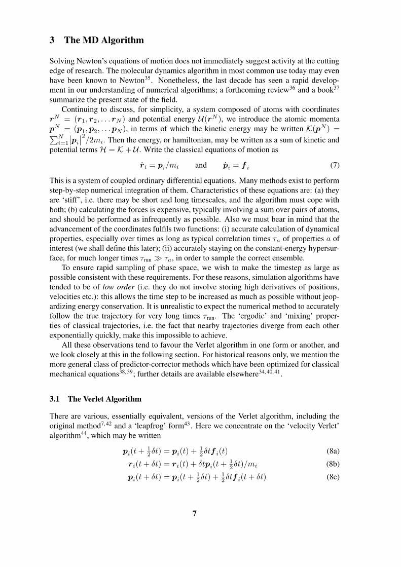
Step (10a) may be implemented by defining unconstrained variables

p(t + 12δt) = p(t) + 1

2δtf(t) , r(t + δt) = r(t) + δtp(t + 12δt)/m

then solving the nonlinear equation for λ

χ(t + δt) = χ(r(t + δt) + λδtg(t)/m

)= 0

and substituting back

p(t + 12δt) = p(t + 1

2δt) + λg(t) , r(t + δt) = r(t + δt) + δtλg(t)/m

Step (10b) may be handled by defining

p(t + δt) = p(t + 12δt) + 1

2δtf(t + δt)

solving the equation for the second Lagrange multiplier µ

χ(t + δt) = χ(r(t + δt), p(t + δt) + µg(t + δt)

)= 0

(which is actually linear, since χ(r, p) = −g(r) · p/m) and substituting back

p(t + δt) = p(δt) + µg(t + δt)

In pseudo-code this scheme may be written

do step = 1, nstepp = p + (dt/2)*fr = r + dt*p/mlambda_g = shake(r)p = p + lambda_gr = r + dt*lambda_g/mf = force(r)p = p + (dt/2)*fmu_g = rattle(r,p)p = p + mu_g

enddo

The routine called shake here calculates the constraint forces λgi necessary to ensure

that the end-of-step positions ri satisfy Eq. (9a). For a system of many constraints, this

calculation is usually performed in an iterative fashion, so as to satisfy each constraint

in turn until convergence; the original SHAKE algorithm was framed in this way. These

constraint forces are incorporated into both the end-of-step positions and the mid-step mo-

menta. The routine called rattle calculates a new set of constraint forces µg i to ensure

that the end-of-step momenta satisfy Eq. (9b). This also may be carried out iteratively.

9

It is important to realize that a simulation of a system with rigidly constrained bond

lengths, is not equivalent to a simulation with, for example, harmonic springs represent-

ing the bonds, even in the limit of very strong springs. A subtle, but crucial, difference

lies in the distribution function for the other coordinates. If we obtain the configurational

distribution function by integrating over the momenta, the difference arises because in one

case a set of momenta is set to zero, and not integrated, while in the other an integration

is performed, which may lead to an extra term depending on particle coordinates. This

is frequently called the ‘metric tensor problem’; it is explained in more detail in the refer-

ences34, 51, and there are well-established ways of determining when the difference is likely

to be significant52 and how to handle it, if necessary53. Constraints also find an application

in the study of rare events51, or for convenience when it is desired to fix, for example, the

director in a liquid crystal simulation54.

An alternative to constraints, is to retain the intramolecular bond potentials and use a

multiple time step approach to handle the fast degrees of freedom. We discuss this shortly.

3.3 Periodic Boundary Conditions

Small sample size means that, unless surface effects are of particular interest, periodic

boundary conditions need to be used. Consider 1000 atoms arranged in a 10 × 10 × 10cube. Nearly half the atoms are on the outer faces, and these will have a large effect on the

measured properties. Even for 106 = 1003 atoms, the surface atoms amount to 6% of the

total, which is still nontrivial. Surrounding the cube with replicas of itself takes care of this

problem. Provided the potential range is not too long, we can adopt the minimum imageconvention that each atom interacts with the nearest atom or image in the periodic array.

In the course of the simulation, if an atom leaves the basic simulation box, attention can

be switched to the incoming image. This is shown in Figure 5. Of course, it is important

to bear in mind the imposed artificial periodicity when considering properties which are

influenced by long-range correlations. Special attention must be paid to the case where the

potential range is not short: for example for charged and dipolar systems.

3.4 Neighbour Lists

Computing the non-bonded contribution to the interatomic forces in an MD simulation

involves, in principle, a large number of pairwise calculations: we consider each atom iand loop over all other atoms j to calculate the minimum image separations rij . Let us

assume that the interaction potentials are of short range, v(rij) = 0 if rij > rcut, the

potential cutoff. In this case, the program skips the force calculation, avoiding expensive

calculations, and considers the next candidate j. Nonetheless, the time to examine all

pair separations is proportional to the number of distinct pairs, 12N(N − 1) in an N -atom

system, and for every pair one must compute at least r2ij ; this still consumes a lot of time.

Some economies result from the use of lists of nearby pairs of atoms. Verlet7 suggested

such a technique for improving the speed of a program. The potential cutoff sphere, of

radius rcut, around a particular atom is surrounded by a ‘skin’, to give a larger sphere of

radius rlist as shown in Figure 6. At the first step in a simulation, a list is constructed of

all the neighbours of each atom, for which the pair separation is within rlist. Over the next

few MD time steps, only pairs appearing in the list are checked in the force routine. From

10

Figure 5. Periodic boundary conditions. As a particle moves out of the simulation box, an image particle moves

in to replace it. In calculating particle interactions within the cutoff range, both real and image neighbours are

included.

Figure 6. The Verlet list on its construction, later, and too late. The potential cutoff range (solid circle), and the

list range (dashed circle), are indicated. The list must be reconstructed before particles originally outside the list

range (black) have penetrated the potential cutoff sphere.

time to time the list is reconstructed: it is important to do this before any unlisted pairs

have crossed the safety zone and come within interaction range. It is possible to trigger the

list reconstruction automatically, if a record is kept of the distance travelled by each atom

since the last update. The choice of list cutoff distance rlist is a compromise: larger lists

11

Figure 7. The cell structure. The potential cutoff range is indicated. In searching for neighbours of an atom, it is

only necessary to examine the atom’s own cell, and its nearest-neighbour cells (shaded).

will need to be reconstructed less frequently, but will not give as much of a saving on cpu

time as smaller lists. This choice can easily be made by experimentation.

For larger systems (N ≥ 1000 or so, depending on the potential range) another tech-

nique becomes preferable. The cubic simulation box (extension to non-cubic cases is pos-

sible) is divided into a regular lattice of ncell × ncell × ncell cells; see Figure 7. These cells

are chosen so that the side of the cell cell = L/ncell is greater than the potential cutoff dis-

tance rcut. If there is a separate list of atoms in each of those cells, then searching through

the neighbours is a rapid process: it is only necessary to look at atoms in the same cell as

the atom of interest, and in nearest neighbour cells. The cell structure may be set up and

used by the method of linked lists55, 43. The first part of the method involves sorting all

the atoms into their appropriate cells. This sorting is rapid, and may be performed every

step. Then, within the force routine, pointers are used to scan through the contents of cells,

and calculate pair forces. This approach is very efficient for large systems with short-range

forces. A certain amount of unnecessary work is done because the search region is cubic,

not (as for the Verlet list) spherical.

4 Time Dependence

A knowledge of time-dependent statistical mechanics is important in three general areas

of simulation. Firstly, in recent years there have been significant advances in the under-

standing of molecular dynamics algorithms, which have arisen out of an appreciation of the

formal operator approach to classical mechanics. Second, an understanding of equilibrium

time correlation functions, their link with dynamical properties, and especially their con-

nection with transport coefficients, is essential in making contact with experiment. Third,

the last decade has seen a rapid development of the use of nonequilibrium molecular dy-

namics, with a better understanding of the formal aspects, particularly the link between the

dynamical algorithm, dissipation, chaos, and fractal geometry. Space does not permit a full

12

description of all these topics here: the interested reader should consult Refs 56,57,51 and

references therein.

The Liouville equation dictates how the classical statistical mechanical distribution

function (rN , pN , t) evolves in time. From considerations of standard, Hamiltonian,

mechanics45 and the flow of representative systems in an ensemble through a particular

region of phase space, it is easy to derive the Liouville equation

∂

∂t= −

∑i

ri ·∂

∂ri+ pi ·

∂

∂pi

≡ −iL , (11)

defining the Liouville operator iL as the quantity in braces. Contrast this equation for

with the time evolution equation for a dynamical variable A(rN , pN ), which comes

directly from the chain rule applied to Hamilton’s equations

A =∑

i

ri ·∂A

∂ri+ pi ·

∂A

∂pi

≡ iLA . (12)

The formal solutions of the time evolution equations are

(t) = e−iLt(0) and A(t) = eiLtA(0) (13)

where, in either case, the exponential operator is called the propagator. A number of ma-

nipulations are possible, once this formalism has been established. There are useful analo-

gies both with the Eulerian and Lagrangian pictures of incompressible fluid flow, and with

the Heisenberg and Schrodinger pictures of quantum mechanics (see e.g. Ref. 58, Chap. 7,

and Ref. 59, Chap. 11). These analogies are particularly useful in formulating the equa-

tions of classical response theory60, linking transport coefficients with both equilibrium

and nonequilibrium simulations56.

The Liouville equation applies to any ensemble, equilibrium or not. Equilibrium means

that should be stationary, i.e. that ∂/∂t = 0. In other words, if we look at any phase-

space volume element, the rate of incoming state points should equal the rate of outflow.

This requires that be a function of the constants of the motion, and especially = (H).Equilibrium also implies d〈A〉/dt = 0 for any A. The extension of the above equations to

nonequilibrium ensembles requires a consideration of entropy production, the method of

controlling energy dissipation (thermostatting) and the consequent non-Liouville nature of

the time evolution56.

4.1 Propagators and the Verlet Algorithm

The velocity Verlet algorithm may be derived by considering a standard approximate

decomposition of the Liouville operator which preserves reversibility and is symplectic(which implies that volume in phase space is conserved). This approach61 has had several

beneficial consequences.

The Liouville operator of equation (13) may be written62

eiLt =(eiLδt

)nstep

approx+ O(nstepδt

3)

where δt = t/nstep and an approximate propagator, correct at short timesteps δt → 0,

appears in the parentheses. This is a formal way of stating what we do in molecular dy-

namics, when we split a long time period t into a large number nstep of small timesteps δt,

13

using an approximation to the true equations of motion over each timestep. It turns out that

useful approximations arise from splitting iL into two parts61

iL = iLp + iLr . (14)

where

iLp =∑

i

pi ·∂

∂pi

=∑

i

f i ·∂

∂pi

(15a)

iLr =∑

i

ri ·∂

∂ri=

∑i

m−1i pi ·

∂

∂ri. (15b)

The following approximation

eiLδt = e(iLp+iLr)δt ≈ eiLpδt/2 eiLrδt eiLpδt/2(16)

is asymptotically exact in the limit δt → 0. For nonzero δt this is an approximation to eiLδt

because in general iLp and iLr do not commute, but it is still exactly time reversible and

symplectic.

Effectively, we are propagating the equation of motion in steps which ignore, in turn,

the kinetic part and the potential part of the hamiltonian. A straightforward derivation51

shows that the effect of each operator on a dynamical variable A(rN , pN

)is to advance,

respectively, the coordinates and the momenta separately:

eiLrδtA(r, p

)= A

(r + m−1pδt, p

)(17a)

eiLpδtA(r, p

)= A

(r, p + fδt

)(17b)

where, to avoid clutter, we have written r, p for rN , pN . It is then easy to see that the three

successive steps embodied in equation (16), with the above choice of operators, generate

the velocity Verlet algorithm.

Such a formal approach may seem somewhat abstract, but has been invaluable in un-

derstanding the excellent performance of Verlet-like algorithms in molecular dynamics,

and in extending the range of algorithms available to us. It may be shown that, although

the trajectories generated by the above scheme are approximate, and will not conserve the

true energy H, nonetheless, they do exactly conserve a “pseudo-hamiltonian” or “shadow

hamiltonian” H which differs from the true one by a small amount (vanishing as δt → 0.

This means that no drift in the energy will occur: the system will remain on a hypersurface

in phase space which is “close” (in the above sense) to the true constant-energy hypersur-

face. Such a stability property is extremely useful in molecular dynamics, since we wish

to sample constant-energy states.

An example may make things clearer. Consider a simple harmonic oscillator63, of

natural frequency ω, representing perhaps an interatomic bond in a diatomic molecule.

The equations of motion are

x = p/m p = −mω2x

For these equations, a few lines of algebra shows that the following shadow hamiltonian

H(x, p) =p2/2m

1 − (ωδt/2)2+ 1

2mω2x2

14

is exactly conserved by the velocity Verlet algorithm. In a phase portrait, the simulated

system remains on a constant-H ellipse which differs only slightly (for small ωδt) from

the true constant-H ellipse. This is illustrated in Fig. 8, where we deliberately choose a

high step size δt = 0.7/ω to accentuate the differences. Note that, even for this value of

δt, the energy conservation is very good (the deviation is O(δt2)). At the same time, the

frequency of oscillation is shifted from the true value, so the trajectories steadily diverge

from each other.

0

1

23

4

5

67

8

-1 -0.5 0 0.5 1x

-1

-0.5

0

0.5

1

p / m

ω

Figure 8. Velocity Verlet algorithm for simple harmonic oscillator with initial conditions x(0) = 1, p(0) = 0.

The outer circle shows the exact trajectory, conserving the true hamiltonian H; the inner ellipse is a contour

of constant shadow hamiltonian H for a (relatively large) timestep δt = 0.7/ω. The circles show the exact

solutions at regular intervals δt; the squares show the corresponding velocity Verlet phase points, connected by

straight sections representing the intermediate steps in the algorithm.

4.2 Multiple Timesteps

An important extension of the MD method allows it to tackle systems with multiple time

scales: for example, molecules which have very strong internal springs representing the

bonds, while interacting externally through softer potentials; molecules having strongly-

varying short-range interactions but more smoothly-varying long-range interactions; or

perhaps molecules consisting of both heavy and light atoms. A simple MD algorithm will

have to adopt a timestep short enough to handle the fastest variables.

An attractive improvement is to handle the fast motions with a shorter timestep64, 61, 65.

A time-reversible Verlet-like multiple-timestep algorithm may be generated using the Li-

ouville operator formalism described above. Here we suppose that there are two types of

15

force in the system: “slow” F i, and “fast” f i. The momentum satisfies pi = f i + F i.

Then we break up the Liouville operator iL = i p + iLp + iLr:

i p =∑

i

F i ·∂

∂pi

(18a)

iLp =∑

i

f i ·∂

∂pi

(18b)

iLr =∑

i

m−1pi ·∂

∂ri(18c)

The propagator approximately factorizes

eiL∆t ≈ ei p∆t/2 ei(Lp+Lr)∆t ei p∆t/2

where ∆t represents a long time step. The middle part is then split again, using the con-

ventional separation, and iterating over small time steps δt = ∆t/nstep:

ei(Lp+Lr)∆t ≈[eiLpδt/2 eiLrδt eiLpδt/2

]nstep.

So the fast-varying forces must be computed many times at short intervals; the slow-

varying forces are used just before and just after this stage, and they only need be calculated

once per long timestep.

This translates into a fairly simple algorithm, based closely on the standard velocity

Verlet method. Written in a Fortran-like pseudo-code, it is as follows. At the start of the

run we calculate both rapidly-varying (f) and slowly-varying (F) forces, then, in the main

loop:

do STEP = 1, NSTEPp = p + (DT/2)*Fdo step = 1, nstep

p = p + (dt/2)*fr = r + dt*p/mf = force(r)p = p + (dt/2)*f

enddoF = FORCE(r)p = p + (DT/2)*F

enddo

The entire simulation run consists of NSTEP long steps; each step consists of nstepshorter sub-steps. DT and dt are the corresponding timesteps, DT = nstep*dt.

A particularly fruitful application, which has been incorporated into computer codes

such as ORAC66, is to split the interatomic force law into a succession of components

covering different ranges: the short-range forces change rapidly with time and require a

short time step, but advantage can be taken of the much slower time variation of the long-

range forces, by using a longer time step and less frequent evaluation for these. Having

said this, multiple-time-step algorithms are still under active study67, and there is some

concern that resonances may occur between the natural frequencies of the system and the

16

various timesteps used in schemes of this kind68, 69. Significant efforts have been made in

recent years to overcome these problems and achieve significant increases in step size by

alternative methods70–72. The area remains one of active research73, 36.

5 Rigid Molecule Rotation

In certain applications, particularly in the simulation of liquid crystals, colloidal systems,

and polymers, it is advantageous to include non-spherical rigid bodies in the molecular

model. This means that we must calculate intermolecular torques as well as forces, and

implement the classical dynamical equations for rotational motion.

If the intermolecular forces are expressed as sums of site-site (or atom-atom) terms,

the conversion of these into centre-of-mass forces, and torques about the centre of mass, is

easily performed. Consider two molecules A and B, centre-of-mass position vectors RA,

RB . Define the intermolecular vector RAB = RA −RB , and suppose that the interaction

potential may be expressed

vAB =∑i∈A

∑j∈B

v(rij)

where i and j are atomic sites in the respective molecules. Then we may compute

force on A due to B: F AB =∑i∈A

∑j∈B

f ij = −F BA

torque on A due to B: NAB =∑i∈A

∑j∈B

riA × f ij

torque on B due to A: NBA =∑i∈A

∑j∈B

rjB × f ji

where riA = ri − RA is the position of site i relative to the centre of molecule A (and

likewise for rjB). Note that NAB = −NBA (a common misconception), but that the

above equations give directly

NAB + NBA + RAB × F AB = 0 (19)

provided the forces satisfy f ij = −f ji and act along the site-site vectors rij . This is

the expression of local angular momentum conservation, which follows directly from the

invariance of the potential energy vAB to a rotation of the coordinate system. (Note, in

passing, that, in periodic boundaries, angular momentum is not globally conserved).

There is also a trend to use rigid-body potentials which are defined explictly in terms

of centre-of-mass positions and molecular orientations. An example is the Gay-Berne

potential74

vGBAB(R, a, b) = 4ε(R, a, b)

[−12 − −6

](20a)

with =R − σ(R, a, b) + σ0

σ0(20b)

which depends upon the molecular axis vectors a and b, and on the direction R and mag-

nitude R of the centre-centre vector RAB , which we write R here and henceforth. The

17

parameter σ0 determines the smallest molecular diameter and there are two orientation-

dependent quantities in the above shifted-Lennard-Jones form: a diameter σ(R, a, b) and

an energy ε(R, a, b). Each quantity depends in a complicated way (not given here) on pa-

rameters characterizing molecular shape and structure. This potential has been extensively

used in the study of molecular liquids and liquid crystals75, 76, 54, 77–79and will be discussed

further in a later chapter80. Generalizations to non-uniaxial rigid bodies81–83 have also been

studied: here, the diameter and energy parameters depend on the full orthogonal orientation

matrices a, b, which convert from space-fixed (xyz) to molecule-fixed (123) coordinates,

and whose rows are the three molecule-fixed orthonormal principal axis vectors aα, bβ ,

α, β = 1, 2, 3.

We go through the following derivation in some detail, as it is seldom presented. A

very common case is when the pair potential may be written in the form84

vAB = vAB

(R, aα · R, bβ · R, aα · bβ

)(21)

i.e. a function of the centre-centre separation R, and all possible scalar products of the unit

vectors R, aα and bβ . Using the chain rule, we may write the force on A:

F AB = −∂vAB

∂R= −∂vAB

∂R

∂R

∂R−

∑e=a,b

∂vAB

∂(e · R)

∂(e · R)

∂R

= −∂vAB

∂RR −

∑e=a,b

∂vAB

∂(e · R)

e − (e · R)R

R. (22)

The sum ranges over all the orientation vectors on both molecules, e = aα, bα. The

derivatives of the potential are easily evaluated, assuming that it has the general form of

Eq. (21). To calculate the torques, we follow the general approach of Ref. 84. Consider

the derivative of vAB with respect to rotation of molecule A through an angle ψ about any

axis n. By definition, this gives:

n · NAB = −∂vAB

∂ψ= −

∑α

∑e=R,b

∂vAB

∂(e · aα)

∂(e · aα)

∂ψ. (23)

The sum is over all combinations of unit vectors (aα, e) for which one, aα, rotates with

the molecule while the other, e = R or bβ , remains stationary. This has the effect45

∂aα

∂ψ= n × aα ⇒ ∂(e · aα)

∂ψ= e · n × aα = −n · e × aα .

Then Eq. (23) gives

n · NAB = n ·∑α

∑e=R,b

∂vAB

∂(e · aα)e × aα . (24)

Choosing n to be each of the coordinate directions in turn allows us to identify every

component of the torque:

NAB =∑α

∑e=R,b

∂vAB

∂(e · aα)e × aα . (25)

18

Writing this out explicitly for molecules A and B:

NAB =∑α

∂vAB

∂(aα · R)R × aα −

∑αβ

∂vAB

∂(aα · bβ)aα × bβ (26a)

NBA =∑

β

∂vAB

∂(bβ · R)R × bβ +

∑αβ

∂vAB

∂(aα · bβ)aα × bβ . (26b)

Note that eqns (22), (26a) and (26b) give NAB + NBA + R × fAB = 0 as before.

If the potential is not (easily) expressible in terms of scalar products, a similar deriva-

tion gives the expressions

fAB = −∂vAB

∂R= −∂vAB

∂RR − ∂vAB

∂R

[1 − RR

R

](27a)

NAB = −∑α

aα × ∂vAB

∂aα(27b)

NBA = −∑

β

bβ × ∂vAB

∂bβ

(27c)

which may be more convenient. Specific examples of the use of these equations in the

context of liquid crystal simulations are given elsewhere85.

Methods for integrating the rotational equations of motion, using a symplectic splitting

method akin to that of section 4.1 have been described elsewhere. These tend to fall into

two categories: those based on the rotation matrix86–88, and those based on quaternion

parameters89. Here, we present briefly the former approach. Consider molecule A, and

drop its identifying suffix. Assuming that the inertia tensor I is diagonal in the frame

defined by the aα vectors, the body-fixed angular momentum vector is defined by π = I·ω,

and the rotation matrix satisfies the equation

da

dt= a · Ω where Ω =

⎛⎝ 0 −ω3 ω2

ω3 0 −ω1

−ω2 ω1 0

⎞⎠

The angular momentum satisfies

dπ

dt= π × I−1π + N

where the torque N is expressed in body-fixed coordinates. Then, the essential idea is to

split the rotational propagator

eiLπδt/2 eiLfreeδt eiLπδt/2

where the first and last components advance the angular momentum, using the computed

torque, and the central part corresponds to free rotation governed by the kinetic energy part

of the hamiltonian. In some special cases, the free rotation problem can be solved exactly,

but in the general case it is split further into three separate rotations, each corresponding to

a single element of the diagonal inertia tensor.

19

6 Molecular Dynamics in Different Ensembles

In this section we briefly discuss molecular dynamics methods in the constant-NV T en-

semble; the reader should be aware that analogous approaches exist for other ensembles,

particularly to simulate at constant pressure or stress.

There are three general approaches to conducting molecular dynamics at constant tem-

perature rather than constant energy. One method, simple to implement and reliable, is

to periodically reselect atomic velocities at random from the Maxwell-Boltzmann distri-

bution90. This is rather like an occasional random coupling with a thermal bath. The

resampling may be done to individual atoms, or to the entire system; some guidance on the

reselection frequency may be found in Ref. 90.

A second approach91, 92, is to introduce an extra ‘thermal reservoir’ variable into the

dynamical equations:

ri = pi/m (28a)

pi = f i − ζpi (28b)

ζ =

∑iα p2

iα/m − gkBT

Q≡ ν2

T

[∑iα p2

iα/m

gkBT− 1

]= ν2

T

[TT

− 1

]. (28c)

Here ζ is a friction coefficient which is allowed to vary in time; Q is a thermal inertia

parameter, which may be replaced by νT , a relaxation rate for thermal fluctuations; g ≈3N is the number of degrees of freedom. T stands for the instantaneous ‘mechanical’

temperature. It may be shown that the distribution function for the ensemble is proportional

to exp−βW where W = H + 123NkBTζ2/ν2

T . These equations lead to the following

time variation of the system energy H =∑

iα p2iα/2m + U , and for the variable W:

H =∑iα

piαpiα/m −∑

fiαriα = −ζ∑iα

p2iα/m

W = −3NkBTζ .

If T > T , i.e. the system is too hot, then the ‘friction coefficient’ ζ will tend to increase;

when it is positive the system will begin to cool down. If the system is too cold, the reverse

happens, and the friction coefficient may become negative, tending to heat the system up

again. In some circumstances, this approach generates non-ergodic behaviour, but this may

be ameliorated by the use of chains of thermostat variables93. Ref. 94 gives an example of

the use of this scheme in a biomolecular simulation.

It is also possible to extend the Liouville operator-splitting approach to generate algo-

rithms for molecular dynamics in these ensembles65. Some care needs to be taken, because

eqns (28) are not hamiltonian, but it turns out to be possible to correct this using a suitable

Poincare transformation95 and to implement the resulting symplectic method in an elegant

fashion96, 36.

7 How Long? How Large?

Molecular dynamics evolves a finite-sized molecular configuration forward in time, in a

step-by-step fashion. There are limits on the typical time scales and length scales that can

20

be investigated and the consequences must be considered in analyzing the results. Simula-

tion runs are typically short: typically t ∼ 103–106 MD steps, corresponding to perhaps a

few nanoseconds of real time, and in special cases extending to the microsecond regime97.

This means that we need to test whether or not a simulation has reached equilibrium be-

fore we can trust the averages calculated in it. Moreover, there is a clear need to subject the

simulation averages to a statistical analysis, to make a realistic estimate of the errors. How

long should we run? This depends on the system and the physical properties of interest.

Suppose one is interested in a variable a, defined such that 〈a〉 = 0. The time correla-

tion function 〈a(t0)a(t0 + t)〉 relates values calculated at times t apart; assuming that the

system is in equilibrium, this function is independent of the choice of time origin and may

be written 〈a(0)a(t)〉. It will decay from an initial value 〈a(0)a(0)〉 ≡⟨a2

⟩to a long-time

limiting value

limt→∞ 〈a(0)a(t)〉 = lim

t→∞ 〈a(0)〉 〈a(t)〉 = 0

as the variables a(0) and a(t) become uncorrelated; this decay occurs over a characteristic

time τa. Formally we may define a correlation time

τa =

∫ ∞

0

dt 〈a(0)a(t)〉 /〈a2〉.

Alternatively, if time correlations decay exponentially at long time, τa may be identified

approximately from the limiting form

〈a(0)a(t)〉 ∝ exp−t/τa .

Similarly, define a spatial correlation function 〈a(0)a(r)〉 relating values computed at

different points r apart. Spatial isotropy allows us to write this as a function of the distance

between the points, r, rather than the vector r: note that this symmetry is broken in a liquid

crystal. Spatial homogeneity, which applies to simple liquids (but not to solids or smectic

liquid crystals) allows us to omit any reference to an absolute origin of coordinates. This

function decays from a short-range nonzero value to zero over a characteristic distance ξa,

the correlation length.

It is almost essential for simulation box sizes L to be large compared with ξa, and for

simulation run lengths τ to be large compared with τa, for all properties of interest a. Only

then can we guarantee that reliably-sampled statistical properties are obtained. Roughly

speaking, the statistical error in a property calculated as an average over a simulation run

of length τ is proportional to√

τa/τ : the time average is essentially a sum of ∼ τ/τa

independent quantities, each an average over time τa. Within the time periods τa, values

of a are highly correlated. A similar statement can be made about properties which are ef-

fectively spatial averages over the simulation box volume L3: root-mean-square variations

of such averages are proportional to√

(ξa/L)3. This means that collective, system-wide

properties deviate by only a relatively small amount from their thermodynamic, large-

system, limiting values; the deviation becomes smaller as the averaging volume increases,

and is also determined by the correlation length.

Near critical points, special care must be taken, in that these inequalities will almost

certainly not be satisfied, and indeed one may see the onset of non-exponential decay of the

correlation functions. In these circumstances a quantitative investigation of finite size ef-

fects and correlation times, with some consideration of the appropriate scaling laws, must

21

be undertaken. Phase diagrams of soft-matter systems often include continuous phase tran-

sitions, or weakly first-order transitions exhibiting significant pre-transitional fluctuations.

One of the most encouraging developments of recent years has been the establishment of

reliable and systematic methods of studying critical phenomena by simulation, although

typically the Monte Carlo method is more useful for this type of study98–100, 34, 101, 51.

8 Conclusions

In this introduction, I have tried to focus on points that seem to me both topical and essen-

tial to the mainstream of complex fluid dynamics. Others might have chosen a different

perspective, or focused on different aspects. Exciting areas which I have had to omit in-

clude the use of molecular dynamics to study rare events, the development of mesoscale

modelling techniques such as dissipative particle dynamics, the incorporation of electronic

degrees of freedom through ab initio molecular dynamics, and the efficient implementation

of simulation algorithms on parallel computers. One could argue that these are advanced

topics, but they are progressively entering the mainstream, and ready-written packages are

steadily removing the need to explain some of the lower-level technical issues which I

have included here. Nonetheless, I am a firm believer in understanding what is happening

“under the hood”, even if one does not intend to become a “mechanic”, and hopefully the

foregoing material will help towards that end.

Acknowledgements

I have learnt much about the development of intermolecular potentials from Mark Wil-

son and members of his group. Guido Germano helped me understand several aspects of

molecular motion and program design. Conversations with Sebastian Reich, Ben Leimkuh-

ler, and others on the subject of algorithms have convinced me that this still very much a

live area. Finally, I wish to acknowledge the ongoing work of the CCP5 community in the

UK.

References

1. G. C. Maitland, M. Rigby, E. B. Smith, and W. A. Wakeham. Intermolecular forces:their origin and determination. Clarendon Press, Oxford, 1981.

2. C. G. Gray and K. E. Gubbins. Theory of molecular fluids. 1. Fundamentals. Claren-

don Press, Oxford, 1984.

3. M. Sprik. Effective pair potentials and beyond. In Michael P. Allen and Dominic J.

Tildesley, editors, Computer simulation in chemical physics, volume 397 of NATOASI Series C, pages 211–259, Dordrecht, 1993. Kluwer Academic Publishers. Pro-

ceedings of the NATO Advanced Study Institute on ‘New Perspectives on Computer

Simulation in Chemical Physics’, Alghero, Sardinia, Italy, September 14–24, 1992.

4. A. J. Stone. The Theory of Intermolecular Forces. Clarendon Press, Oxford, 1996.

5. Michael P. Allen, Glenn T. Evans, Daan Frenkel, and Bela Mulder. Hard convex body

fluids. Adv. Chem. Phys., 86:1–166, 1993.

22

6. A. Rahman. Correlations in the motion of atoms in liquid argon. Phys. Rev. A,

136:405–411, 1964.

7. L. Verlet. Computer experiments on classical fluids. i. thermodynamical properties

of Lennard-Jones molecules. Phys. Rev., 159:98–103, 1967.

8. J. Weeks, D. Chandler, and H. C. Andersen. Role of repulsive forces in determining

the equilibrium structure of simple liquids. J. Chem. Phys., 54:5237–5247, 1971.

9. C. Holm. Dealing with long range interactions: Polyelectrolytes. In ComputationalSoft Matter: From Synthetic Polymers to Proteins, 2004. this volume.

10. S. L. Price. Toward more accurate model intermolecular potentials for organic

molecules. Rev. Comput. Chem., 14:225–289, 2000.

11. N. L. Allinger, Y. H. Yuh, and J.-H. Lii. Molecular mechanics - the MM3 force-field

for hydrocarbons. 1. J. Am. Chem. Soc., 111:8551–8566, 1989.

12. J.-H. Lii and N. L. Allinger. Molecular mechanics - the MM3 force-field for hy-

drocarbons. 2. Vibrational frequencies and thermodynamics. J. Am. Chem. Soc.,111:8566–8575, 1989.

13. J.-H. Lii and N. L. Allinger. Molecular mechanics - the MM3 force-field for hydro-

carbons. 3. the Van der Waals potentials and crystal data for aliphatic and aromatic

hydrocarbons. J. Am. Chem. Soc., 111:8576–8582, 1989.

14. N. L. Allinger, K. S. Chen, and J.-H. Lii. An improved force field (MM4) for saturated

hydrocarbons. J. Comput. Chem., 17:642–668, 1996.

15. N. Nevins, K. S. Chen, and N. L. Allinger. Molecular mechanics (MM4) calculations

on alkenes. J. Comput. Chem., 17:669–694, 1996.

16. N. Nevins, J.-H. Lii, and N. L. Allinger. Molecular mechanics (MM4) calculations

on conjugated hydrocarbons. J. Comput. Chem., 17:695–729, 1996.

17. S. J. Weiner, P. A. Kollman, D. A. Case, U. C. Singh, C. Ghio, G. Alagona, S. Profeta,

and P. Weiner. A new force-field for molecular mechanical simulation of nucleic acids

and proteins. J. Am. Chem. Soc., 106:765–784, 1984.

18. W. D. Cornell, P. Cieplak, C. I. Bayly, I. R. Gould, K. M. Merz, D. M. Ferguson, D. C.

Spellmeyer, T. Fox, J. W. Caldwell, and P. A. Kollman. A 2nd generation force-field

for the simulation of proteins, nucleic-acids, and organic molecules. J. Am. Chem.Soc., 117:5179–5197, 1995.

19. B. R. Brooks, R. E. Bruccoleri, B. D. Olafson, D. J States, S. Swaminathan, and

M. Karplus. CHARMM - A program for macromolecular energy, minimization, and

dynamics calculations. J. Comput. Chem., 4:187–217, 1983.

20. W. L. Jorgensen, D. S. Maxwell, and J. TiradoRives. Development and testing of

the OPLS all-atom force field on conformational energetics and properties of organic

liquids. J. Am. Chem. Soc., 118:11225–11236, 1996.

21. M. J. Field. A Practical Introduction to the Simulation of Molecular Systems. Cam-

bridge University Press, Cambridge, 1999.

22. A. R. Leach. Molecular Modelling: Principles and Applications. Prentice Hall, 2nd

edition, 2001.

23. H.-D. Holtje, G. Folkers, W. Sippl, and D. Rognan. Molecular Modeling: BasicPrinciples and Applications. Wiley-VCH, 2003.

24. K. Kremer and G. S. Grest. Dynamics of entangled linear polymer melts - a molecular

dynamics simulation. J. Chem. Phys., 92:5057–5086, 1990.

25. B. Chen, M. G. Martin, and J. I. Siepmann. Thermodynamic properties of the

23

williams, opls-aa, and mmff94 all- atom force fields for normal alkanes. J. Phys.Chem. B, 102:2578–2586, 1998.

26. S. K. Nath, F. A. Escobedo, and J. J. de Pablo. On the simulation of vapor-liquid

equilibria for alkanes. J. Chem. Phys., 108:9905–9911, 1998.

27. M. G. Martin and J. I. Siepmann. Transferable potentials for phase equilibria. 1.

united-atom description of n-alkanes. J. Phys. Chem. B, 102:2569–2577, 1998.

28. J. R. Errington and A. Z. Panagiotopoulos. A new intermolecular potential model for

the n-alkane homologous series. J. Phys. Chem. B, 103:6314–6322, 1999.

29. M. Tsige, J. G. Curro, G. S. Grest, and J. D. McCoy. Molecular dynamics simulations

and integral equation theory of alkane chains: comparison of explicit and united atom

models. Macromolecules, 36:2158–2164, 2003.

30. E. Garcia, M. A. Glaser, N. A. Clark, and D. M. Walba. HFF: a force field for liquid

crystal molecules. J. Molec. Struc. - THEOCHEM, 464:39–48, 1999.

31. D. Reith, H. Meyer, and F. Muller-Plathe. CG-OPT: A software package for automatic

force field design. Comput. Phys. Commun., 148:299–313, 2002.

32. D. Reith, M. Putz, and F. Muller-Plathe. Deriving effective mesoscale potentials from

atomistic simulations. J. Comput. Chem., 24:1624–1636, 2003.

33. M. Putz, K. Kremer, and G. S. Grest. What is the entanglement length in a polymer

melt? Europhys. Lett., 49:735–741, 2000.

34. Michael P. Allen and Dominic J. Tildesley. Computer simulation of liquids. Claren-

don Press, Oxford, hardback, 385pp edition, 1987.

35. E. Hairer, C. Lubich, and Gerhard Wanner. Geometric numerical integration illus-

trated by the Stormer-Verlet method. Acta Numerica., 12:399–450, 2003.

36. C. J. Cotter and S. Reich. Time stepping algorithms for classical molecular dynamics.

In M. Rieth and W. Schommers, editors, Computational Nanotechnology. American

Scientific Publishers. to appear.

37. B. Leimkuhler and S. Reich. Geometric Numerical methods for Hamiltonian Me-chanics. Cambridge University Press, Cambridge, 2004. in press.

38. C. W. Gear. The numerical integration of ordinary differential equations of various

orders. ANL 7126, Argonne National Laboratory, 1966.

39. C. W. Gear. Numerical initial value problems in ordinary differential equations.

Prentice-Hall, Englewood Cliffs, NJ, 1971.

40. J. M. Haile. Molecular dynamics simulation: elementary methods. Wiley, New York,

1992.

41. D. C. Rapaport. The art of molecular dynamics simulation. Cambridge University

Press, 1995.

42. L. Verlet. Computer experiments on classical fluids. ii. equilibrium correlation

functions. Phys. Rev., 165:201–214, 1968.

43. R. W. Hockney and J. W. Eastwood. Computer simulations using particles. Adam

Hilger, Bristol, 1988.

44. W. C. Swope, H. C. Andersen, P. H. Berens, and K. R. Wilson. A computer simulation

method for the calculation of equilibrium constants for the formation of physical clus-

ters of molecules: application to small water clusters. J. Chem. Phys., 76:637–649,

1982.

45. H. Goldstein. Classical Mechanics. Addison Wesley, Reading, Massachusetts, sec-

ond edition, 1980.

24

46. S. W. Deleeuw, J. W. Perram, and H. G. Petersen. Hamilton equations for constrained

dynamic systems. J. Stat. Phys., 61:1203–1222, 1990.

47. J-P. Ryckaert, G. Ciccotti, and H. J. C. Berendsen. Numerical integration of the

cartesian equations of motion of a system with constraints: molecular dynamics of

n-alkanes. J. Comput. Phys., 23:327–341, 1977.

48. G. Ciccotti, M. Ferrario, and J.-P. Ryckaert. Molecular dynamics of rigid systems in

cartesian coordinates. a general formulation. Molec. Phys., 47:1253–1264, 1982.

49. G. Ciccotti and J. P. Ryckaert. Molecular dynamics simulation of rigid molecules.

Comput. Phys. Rep., 4:345–392, 1986.

50. H. C. Andersen. Rattle: a “velocity” version of the shake algorithm for molecular

dynamics calculations. J. Comput. Phys., 52:24–34, 1983.

51. D. Frenkel and B. Smit. Understanding molecular simulation : from algorithms toapplications. Academic Press, San Diego, 2nd edition, 2002.

52. W. F. van Gunsteren. Constrained dynamics of flexible molecules. Molec. Phys.,40:1015–1019, 1980.

53. M. Fixman. Classical statistical mechanics of constraints: a theorem and application

to polymers. Proc. Nat. Acad. Sci., 71:3050–3053, 1974.

54. Michael P. Allen, Mark A. Warren, Mark. R. Wilson, Alain Sauron, and William

Smith. Molecular dynamics calculation of elastic constants in Gay-Berne nematic

liquid crystals. J. Chem. Phys., 105:2850–2858, 1996.

55. D. Knuth. The art of computer programming. Addison-Wesley, Reading MA, 2nd

edition, 1973.

56. D. J. Evans and G. P. Morriss. Statistical Mechanics of Nonequilibrium Liquids.

Academic Press, London, 1990.

57. B. L. Holian. The character of the nonequilibrium steady state: beautiful formalism

meets ugly reality. In K. Binder and G. Ciccotti, editors, Monte Carlo and moleculardynamics of condensed matter systems, volume 49, pages 791–822. Italian Physical

Society, Bologna, 1996. Proceedings of the Euroconference on ‘Monte Carlo and

molecular dynamics of condensed matter systems’, Como, Italy, July 3–28, 1995.

58. L. E. Reichl. A modern course in Statistical Physics. University of Texas Press,

Austin, 1980.

59. H. L. Friedman. A course in statistical mechanics. Prentice-Hall, Englewood Cliffs,

NJ., 1985.

60. B. L. Holian and D. J. Evans. Classical response theory in the Heisenberg picture. J.Chem. Phys., 83:3560–3566, 1985.

61. M. Tuckerman, B. J. Berne, and G. J. Martyna. Reversible multiple time scale molec-

ular dynamics. J. Chem. Phys., 97:1990–2001, 1992.

62. H. F. Trotter. Proc. Amer. Math. Soc., 10:545, 1959.

63. S. Toxvaerd. Hamiltonians for discrete dynamics. Phys. Rev. E, 50:2271–2274, 1994.

64. H. Grubmuller, H. Heller, A. Windemuth, and K. Schulten. Generalized Verlet al-

gorithm for efficient molecular dynamics simulations with long-range interactions.

Molec. Simul., 6:121, 1991.

65. G. J. Martyna, M. E. Tuckerman, D. J. Tobias, and M. L. Klein. Explicit reversible

integrators for extended systems dynamics. Molec. Phys., 87:1117–1157, 1996.

66. P. Procacci, T. A. Darden, E. Paci, and M. Marchi. ORAC: A molecular dynamics

program to simulate complex molecular systems with realistic electrostatic interac-

25

tions. J. Comput. Chem., 18:1848–1862, 1997.

67. P. Deuflhard, J. Hermans, B. Leimkuhler, A. E. Mark, S. Reich, and R. D. Skeel,

editors. Computational Molecular Dynamics: Challenges, Methods, Ideas, volume 4

of Lect. Notes Comp. Sci. Eng. Springer, Berlin, 1998.

68. T. Schlick, M. Mandziuk, R. D. Skeel, and K. Srinivas. Nonlinear resonance artifacts

in molecular dynamics simulations. J. Comput. Phys., 140:1–29, 1998.

69. Q. Ma, J. A. Izaguirre, and R. D. Skeel. Verlet-I/r-RESPA/Impulse is limited by

nonlinear instabilities. S.I.A.M. J. Sci. Comput., 24:1951–1973, 2003.

70. B. Garcia-Archilla, J. M. Sanz-Serna, and R. D. Skeel. Long-time-step methods for

oscillatory differential equations. S.I.A.M. J. Sci. Comput., 20:930–963, 1998.

71. J. A. Izaguirre, S. Reich, and R. D. Skeel. Longer time steps for molecular dynamics.

J. Chem. Phys., 110:9853–9864, 1999.

72. J. A. Izaguirre, D. P. Catarello, J. M. Wozniak, and R. D. Skeel. Langevin stabilization

of molecular dynamics. J. Chem. Phys., 114:2090–2098, 2001.

73. T. Schlick, R. D. Skeel, A. T. Brunger, L. V. Kale, J. A. Board, J. Hermans, and

K. Schulten. Algorithmic challenges in computational molecular biophysics. J.Comput. Phys., 151:9–48, 1999.

74. J. G. Gay and B. J. Berne. Modification of the overlap potential to mimic a linear

site-site potential. J. Chem. Phys., 74:3316–3319, 1981.

75. E. de Miguel, L. F. Rull, M. K. Chalam, and K. E. Gubbins. Liquid crystal phase

diagram of the Gay-Berne fluid. Molec. Phys., 74:405–424, 1991.

76. R. Berardi, A. P. J. Emerson, and C. Zannoni. Monte Carlo investigations of a Gay-

Berne liquid crystal. J. Chem. Soc. Faraday Trans., 89:4069–4078, 1993.

77. M. A. Bates and G. R. Luckhurst. Computer simulation studies of anisotropic sys-

tems. 26. Monte Carlo investigations of a Gay-Berne discotic at constant pressure. J.Chem. Phys., 104:6696–6709, 1996.

78. M. R. Wilson. Molecular dynamics simulations of flexible liquid crystal molecules

using a Gay-Berne / Lennard-Jones model. J. Chem. Phys., 107:8654–8663, 1997.

79. J. L. Billeter and R. A. Pelcovits. Simulations of liquid crystals. Comput. Phys.,12:440–448, 1998.

80. M. P. Allen. Liquid crystal systems. In Computational Soft Matter: From SyntheticPolymers to Proteins, 2004. this volume.

81. R. Berardi, C. Fava, and C. Zannoni. A generalized Gay-Berne intermolecular poten-

tial for biaxial particles. Chem. Phys. Lett., 236:462–468, 1995.

82. D. J. Cleaver, C. M. Care, M. P. Allen, and M. P. Neal. Extension and generalization

of the Gay-Berne potential. Phys. Rev. E, 54:559–567, 1996.

83. R. Berardi, C. Fava, and C. Zannoni. A Gay-Berne potential for dissimilar biaxial

particles. Chem. Phys. Lett., 297:8–14, 1998.

84. S. L. Price, A. J. Stone, and M. Alderton. Explicit formulae for the electrostatic

energy, forces and torques between a pair of molecules of arbitrary symmetry. Molec.Phys., 52:987–1001, 1984.

85. M. P. Allen and G. Germano. Rigid body potentials, forces and torques. Technical

report, University of Warwick, 2002.

http://eprints.csc.warwick.ac.uk/archive/00000064/.

86. A. Dullweber, B. Leimkuhler, and R. McLachlan. Symplectic splitting methods for

rigid body molecular dynamics. J. Chem. Phys., 107:5840–5851, 1997.

26

87. A. Kol, B. B. Laird, and B. J. Leimkuhler. A symplectic method for rigid-body

molecular simulation. J. Chem. Phys., 107:2580–2588, 1997.

88. T. Holder, B. Leimkuhler, and S. Reich. Explicit variable step-size and time-reversible

integration. Appl. Numer. Math., 39:367–377, 2001.

89. T. F. Miller, M. Eleftheriou, P. Pattnaik, A. Ndirango, D. Newns, and G. J. Martyna.

Symplectic quaternion scheme for biophysical molecular dynamics. J. Chem. Phys.,116:8649–8659, 2002.

90. H. C. Andersen. Molecular dynamics simulations at constant pressure and/or temper-

ature. J. Chem. Phys., 72:2384–2393, 1980.

91. S. Nose. A molecular dynamics method for simulations in the canonical ensemble.

Molec. Phys., 52:255–268, 1984.

92. W. G. Hoover. Canonical dynamics - equilibrium phase-space distributions. Phys.Rev. A, 31:1695–1697, 1985.

93. G. J. Martyna, M. L. Klein, and M. Tuckerman. Nose-Hoover chains: the canonical

ensemble via continuous dynamics. J. Chem. Phys., 97:2635–2643, 1992.

94. D. J. Tobias, G. J. Martyna, and M. L. Klein. Molecular dynamics simulations of a

protein in the canonical ensemble. J. Phys. Chem., 97:12959–12966, 1993.

95. S. D. Bond, B. J. Leimkuhler, and B. B. Laird. The nose-poincare method for constant

temperature molecular dynamics. J. Comput. Phys., 151:114–134, 1999.

96. S. Nose. An improved symplectic integrator for nose-poincare thermostat. J. Phys.Soc. Japan, 70:75–77, 2001.

97. Y. Duan and P. A. Kollman. Pathways to a protein folding intermediate observed in a

1-microsecond simulation in aqueous solution. Science, 282:740–744, 1998.

98. H. Muller-Krumbhaar and K. Binder. Dynamic properties of the Monte-Carlo method

in statistical mechanics. J. Stat. Phys., 8:1–24, 1973.

99. A. M. Ferrenberg, D. P. Landau, and K. Binder. Statistical and systematic errors in

Monte-Carlo sampling. J. Stat. Phys., 63:867–882, 1991.

100. K. Binder, editor. The Monte Carlo Method in Condensed Matter Physics, volume 71

of Topics Appl. Phys. Springer, Berlin, 2nd edition, 1995.

101. D. P. Landau and K. Binder. A Guide to Monte Carlo Simulations in StatisticalPhysics. Cambridge University Press, Cambridge, 2000.

27