Introduction to nonlinear geometric PDEs - ETH Z€¦ · · 2014-01-20Introduction to nonlinear...

Introduction to nonlinear geometric PDEs

Thomas Marquardt

January 16, 2014

ETH ZurichDepartment of Mathematics

Contents

I. Introduction and review of useful material 1

1. Introduction 31.1. Scope of the lecture . . . . . . . . . . . . . . . . . . . . . . . . . . . . . . 31.2. Accompanying books . . . . . . . . . . . . . . . . . . . . . . . . . . . . . . 41.3. A historic survey . . . . . . . . . . . . . . . . . . . . . . . . . . . . . . . . 5

2. Review: Differential geometry 72.1. Hypersurfaces in Rn . . . . . . . . . . . . . . . . . . . . . . . . . . . . . . 72.2. Isometric immersions . . . . . . . . . . . . . . . . . . . . . . . . . . . . . . 112.3. First variation of area . . . . . . . . . . . . . . . . . . . . . . . . . . . . . 12

3. Review: Linear PDEs of second order 153.1. Elliptic PDEs in Holder spaces . . . . . . . . . . . . . . . . . . . . . . . . 153.2. Elliptic PDEs in Sobolev spaces . . . . . . . . . . . . . . . . . . . . . . . . 183.3. Parabolic PDEs in Holder spaces . . . . . . . . . . . . . . . . . . . . . . . 20

II. Nonlinear elliptic PDEs of second order 25

4. General theory for quasilinear problems 274.1. Fixed point theorems: From Brouwer to Leray-Schauder . . . . . . . . . . 274.2. Reduction to a priori estimates in the C1,β-norm . . . . . . . . . . . . . . 294.3. Reduction to a priori estimates in the C1-norm . . . . . . . . . . . . . . . 30

5. The prescribed mean curvature problem 335.1. C0-estimate . . . . . . . . . . . . . . . . . . . . . . . . . . . . . . . . . . . 335.2. Interior gradient estimate . . . . . . . . . . . . . . . . . . . . . . . . . . . 375.3. Boundary gradient estimate . . . . . . . . . . . . . . . . . . . . . . . . . . 405.4. Existence and uniqueness theorem . . . . . . . . . . . . . . . . . . . . . . 45

6. General theory for fully nonlinear problems 496.1. Fully nonlinear Dirichlet problems . . . . . . . . . . . . . . . . . . . . . . 506.2. Fully nonlinear oblique derivative problems . . . . . . . . . . . . . . . . . 52

7. The capillary surface problem 577.1. C0-estimate . . . . . . . . . . . . . . . . . . . . . . . . . . . . . . . . . . . 587.2. Global gradient estimate . . . . . . . . . . . . . . . . . . . . . . . . . . . . 607.3. Existence and uniqueness theorem . . . . . . . . . . . . . . . . . . . . . . 66

III. Geometric evolution equations 67

8. Classical solutions of MCF and IMCF 698.1. Short-time existence . . . . . . . . . . . . . . . . . . . . . . . . . . . . . . 698.2. Evolving graphs under mean curvature flow . . . . . . . . . . . . . . . . . 748.3. A Neumann problem for inverse mean curvature flow . . . . . . . . . . . . 79

9. Outlook: Level set flow and weak solutions of (I)MCF 939.1. Derivation of the level set problem . . . . . . . . . . . . . . . . . . . . . . 939.2. Solving the level set problem . . . . . . . . . . . . . . . . . . . . . . . . . 94

Bibliography 95

Preface

These notes are the basis for an introductory lecture about geometric PDEs at ETHZurich in the spring term 2013. The course is based on my diploma thesis about pre-scribed mean curvature problems, my PhD thesis about inverse mean curvature flow andmany inspiring lectures by my former thesis advisor Gerhard Huisken.

Further information about the lecture can be found on the course web page:

www.math.ethz.ch/education/bachelor/lectures/hs2013/math/PDEs

If you have questions or comments please feel free to contact me:

[email protected].

I want to thank Malek Alouini, Andreas Leiser and Mario Schulz for very valuable sug-gestions.

i

Part I.

Introduction and review of usefulmaterial

1

1. Introduction

1.1. Scope of the lecture

Geometric analysis is a field that has considerably grown over the last decades. Its goalis to answer questions that arise in geometry, topology, physics and many other sciences(e.g. in image processing) with the help of analytic tools. Usually the first task is tomodel the problem in terms of a (system of) PDE(s)1. Then existence and uniquenessis investigated using tools from PDE theory and/or the calculus of variations as well asfunctional analytic tools. Most of the time the geometric objects under consideration arenot at all smooth. This requires the language of geometric measure theory to treat thoseproblems.

The aim of the course is to give an introduction to the field of nonlinear geometric PDEsby discussing two typical classes of PDEs. For the first part of the course we will dealwith nonlinear elliptic problems. In particular, we will look at the Dirichlet problem ofprescribed mean curvature and the corresponding Neumann problem of capillary surfaces.In the second part we will investigate nonlinear parabolic PDEs. As an example we willdiscuss the evolution of surfaces under inverse mean curvature flow. We will prove short-time existence as well as convergence results and introduce the notion of weak solutions.

Prescribing the scalar mean curvature H of a hypersurface Mn ⊂ Rn+1 which is givenas the graph of a scalar function u : Ω ⊂ Rn → R leads to the following equation2:

div(

Du√1 + |Du|2

)= H(·, u,Du) in Ω. (1.1)

Together with a Dirichlet boundary condition u = φ on ∂Ω equation (1.1) is called theprescribed mean curvature problem. If we consider Neumann boundary conditions, i.e.if we prescribe the boundary contact angle the problem goes under the name capillarysurface equation. During the first part of the course we will discuss existence and unique-ness of solutions to those problems. Note that if the denominator in (1.1) is replaced byone we obtain the Laplace operator. We will use the knowledge about linear second orderelliptic PDEs together with a fixed point argument (or the method of continuity) and apriori estimates to prove existence for the corresponding nonlinear problems.

In the same way as the prescribed mean curvature equation resembles the Poissonequation, the evolution equation for the deformation of a hypersurface Mn ⊂ Nn+1 intime will resemble the heat equation. In our discussion we will focus on a deformationof hypersurfaces Mn along their inverse mean curvature. In terms of the embedding

1This step is not at all unique. People have come up with totally different successful models to answerexactly the same questions.

2We will discuss this in more detail in Section 2.1

3

4 1. Introduction

F : Mn × [0, T ]→ Nn+1 the equation reads

∂F

∂t= 1Hν F : Mn × [0, T )→ (Nn+1, g). (1.2)

The similarity to the heat equation will become clear during the second part of the course.The investigation of (1.2) will lead us to the topic of nonlinear parabolic PDEs. We willanalyze their well-posedness (i.e. short-time existence) as well as their long-time behavior.Finally we will also discuss the construction of weak solutions via the level set method.It turns out this procedure brings us back to a degenerate version of (1.1).

1.2. Accompanying booksThe following books contain subjects which are relevant for the topics we will discussduring the semester. We will not follow a particular book. However, for the first part ofthe course the book by Gilbarg and Trudinger will be closest to the lecture notes. Forthe second part the book by Gerhardt might be the most relevant one.

Overview about the field of PDEs:

• Evans [17]

Elliptic PDEs of second order:

• Gilbarg, Trudinger [23]

• Ladyzenskaja, Ural’ceva [37]

Parabolic PDEs of second order:

• Lieberman [40]

• Ladyzenskaja, Solonnikov, Ural’ceva [38]

Maximum principle:

• Protter, Weinberger [53]

Minimal surfaces:

• Giusti [24]

• Dierkes, Hildebrand, Sauvigny [10]

Mean curvature flow and related flows:

• Gerhardt [22]

• Ecker [11]

• Ritore, Sinestrari [54]

• Mantegazza, C. [41]

1.3. A historic survey 5

1.3. A historic surveyThe field of geometric analysis is becoming more and more active during the last years.To give you an idea about the developments I made a brief survey in form of importantresults over the last 80 years. Note that the books and articles I cited here are not alwayswritten by the people who proved the result. If available I chose review articles whichgive an easy introduction into the topic.

1930: The Plateau problemSolved independently by Douglas and Rado in 1930:

• Dierkes, Hildebrand, Sauvigny [10]

1979: The positive mass theoremProved by Schoen and Yau:

• Schoen (in Proc. of the Clay summer school 2001) [30]

1984: The Yamabe problemPartial results by Trudinger, Aubin and others, finally solved by Schoen:

• Lee, Parker [39]

• Struwe [61]

• Bar [3]

1999: The Penrose inequalityRiemannian version proved by Huisken and Ilmanen and in a bit more general versiontwo years later by Bray. The full Penrose inequality is still an open problem:

• Bray [5]

2002: The double bubble conjectureProved by Hutchings, Morgan, Ritore and Ros.

• Morgan [47]

2003: The Poincare conjectureProved by Perelman based on Hamilton’s work on the Ricci flow:

• Ecker [12]

• Morgan, Tian [48]

2007: The differentiable sphere theoremProved by Brendle and Schoen:

• Brendle [6]

2012: The Lawson conjectureProved by Brendle:

• Brendle [7]

6 1. Introduction

2012: The Wilmore conjectureProved by Marques and Neves:

• Marques, Neves [45]

Of course the list can not be complete. But if you have the feeling I missed somethingvery important please let me know.

2. Review: Differential geometry

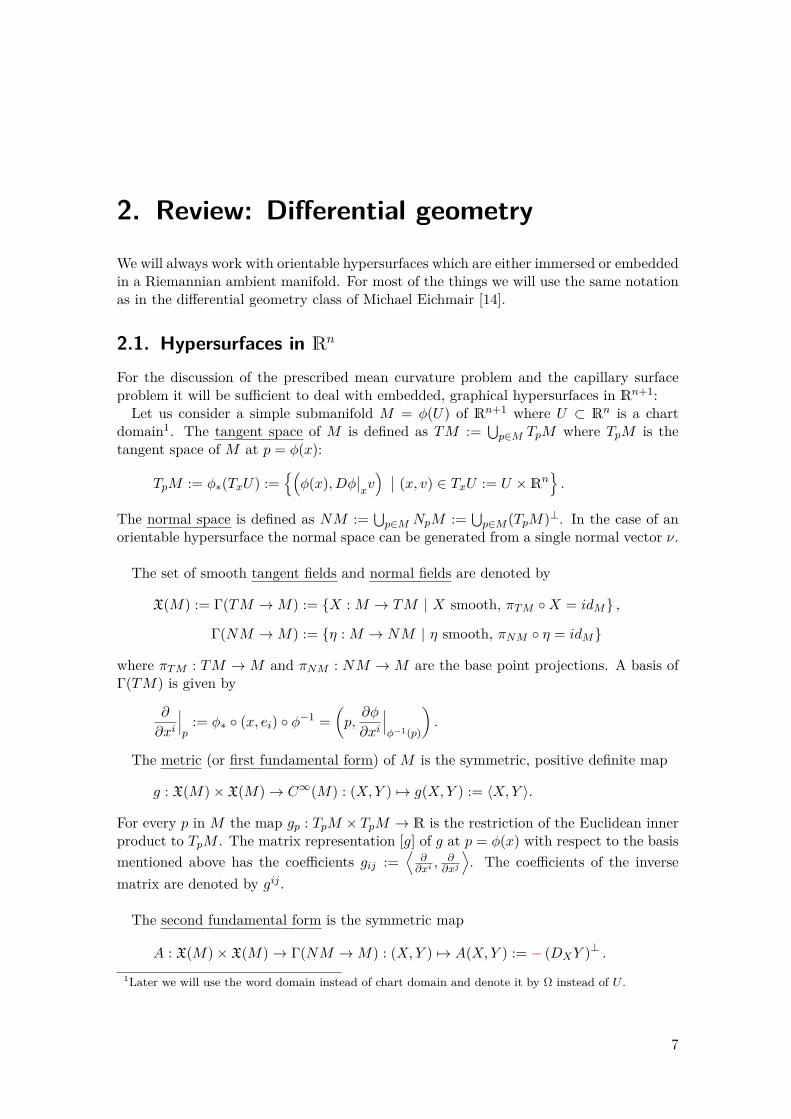
We will always work with orientable hypersurfaces which are either immersed or embeddedin a Riemannian ambient manifold. For most of the things we will use the same notationas in the differential geometry class of Michael Eichmair [14].

2.1. Hypersurfaces in Rn

For the discussion of the prescribed mean curvature problem and the capillary surfaceproblem it will be sufficient to deal with embedded, graphical hypersurfaces in Rn+1:

Let us consider a simple submanifold M = φ(U) of Rn+1 where U ⊂ Rn is a chartdomain1. The tangent space of M is defined as TM :=

⋃p∈M TpM where TpM is the

tangent space of M at p = φ(x):

TpM := φ∗(TxU) :=(φ(x), Dφ

∣∣xv) ∣∣ (x, v) ∈ TxU := U ×Rn

.

The normal space is defined as NM :=⋃p∈M NpM :=

⋃p∈M (TpM)⊥. In the case of an

orientable hypersurface the normal space can be generated from a single normal vector ν.

The set of smooth tangent fields and normal fields are denoted by

X(M) := Γ(TM →M) := X : M → TM | X smooth, πTM X = idM ,

Γ(NM →M) := η : M → NM | η smooth, πNM η = idM

where πTM : TM → M and πNM : NM → M are the base point projections. A basis ofΓ(TM) is given by

∂

∂xi

∣∣∣p

:= φ∗ (x, ei) φ−1 =(p,∂φ

∂xi

∣∣∣φ−1(p)

).

The metric (or first fundamental form) of M is the symmetric, positive definite map

g : X(M)× X(M)→ C∞(M) : (X,Y ) 7→ g(X,Y ) := 〈X,Y 〉.

For every p in M the map gp : TpM × TpM → R is the restriction of the Euclidean innerproduct to TpM . The matrix representation [g] of g at p = φ(x) with respect to the basismentioned above has the coefficients gij :=

⟨∂∂xi, ∂∂xj

⟩. The coefficients of the inverse

matrix are denoted by gij .

The second fundamental form is the symmetric map

A : X(M)× X(M)→ Γ(NM →M) : (X,Y ) 7→ A(X,Y ) := − (DXY )⊥ .1Later we will use the word domain instead of chart domain and denote it by Ω instead of U .

7

8 2. Review: Differential geometry

where D is the (covariant) derivative on TRn+1. We obtain2

A(X,Y ) = −〈DXY, ν〉ν =: h(X,Y )ν

The coefficients of the matrix [h] with respect to the basis mentioned above are hij =⟨−D ∂

∂xi

∂∂xj

, ν

⟩. The Eigenvalues of [g]−1[h] are called principle curvatures. Their sum

is called mean curvature and their product is called Gaussian curvature.

Exercise I.1 (Geometric meaning of the principal curvatures). LetM be a smoothsurface in R3 with unit normal ν. Let ε > 0 and γ : (−ε, ε)→M be a smooth curve suchthat γ(0) = p and γ′(0) = v with |v| = 1. We define the curvature of M at p in directionv as

kp : TpM → R : v 7→ kp(v) := 〈γ′′(0), ν〉.

Note that by Meusnier’s theorem kp is well defined. Answer the following questions

(i) Why does it make sense to call kp the curvature of M at p in dir. v?(ii) What is the relation between kp and h?(iii) What are the critical values of kp in terms of h and g?

The tangential covariant derivative on TM is defined as

∇ : X(M)× X(M)→ X(M) : (X,Y ) 7→ ∇XY := (DXY )>

where (∇XY )(p) := ∇X(p)Y = (DX(p)Y )>. For computations the Leibniz rule and metriccompatibility are important tools

∇XfY = (Xf)Y + f∇XY, Zg(X,Y ) = g(∇ZX,Y ) + g(X,∇ZY )

for all X,Y, Z ∈ Γ(TM) and f ∈ C∞(M). Recall that

Xf = Xi ∂

∂xif := Xi∂(f φ)

∂xi

∣∣∣φ−1

.

where ∂∂xi

is used as a symbol for the basis element as well as for the actual partial deriva-tive in Rn.

The functions Γkij such that ∇ ∂

∂xi

∂∂xj

= Γkij ∂∂xk

are called Christoffel symbols. It is notdifficult to verify that

Γkij = 12g

kl(∂gil∂xj

+ ∂glj∂xi− ∂gij∂xl

).

It follows that for X = Xi ∂∂xi, Y = Y j ∂

∂xjwe have

∇XY = Xi

(∂Y k

∂xi+ Y jΓkij

)∂

∂xk.

2Note that the sign of h depends on the choice of normal ν.

2.1. Hypersurfaces in Rn 9

Based on the rules that taking covariant derivatives commutes with contractions andthat ∇X(S⊗T ) = (∇XS)⊗T+S⊗(∇XT ) we obtain connections on the associated vectorbundles. For example, for differential one forms we get (∇Xω)Y = Xω(Y ) − ω(∇XY ).In coordinates, i.e. X = Xi ∂

∂xi, ω = ωkdx

k this yields

∇Xω = Xi(∂ωk∂xi− ωjΓjik

)dxk.

The tangential gradient of a function f ∈ C∞(M) is defined to be the unique tangentfield3 gradM f such that g(gradM f,X) = df(X) = Xf for all X in Γ(TM). We obtainthe formulae

gradM f = gij∂f

∂xi∂

∂xj= gradRn+1 f − 〈gradRn+1 f, ν〉 ν =

m∑i=1

(Dτif)τi

where we used an orthonormal frame (τi) of TM in the last equality.The tangential divergence of a tangent field X can be defined via the contraction of∇X. We can write

divM X :=n∑i=1

(∂Xi

∂xi+ ΓiijXj

)= divRn+1 X − 〈DνX, ν〉 =

m∑i=1〈DτiX, τi〉

using once more an orthonormal frame of TM for the last expression. Note that the lasttwo equalities also make sense for vector fields which are not necessarily tangential.

In the special case ω = df = ∂f∂xidxi we obtain the Hessian of f :

(HessM f)(X,Y ) = (∇df)(X,Y ) = (∇Xdf)(Y ) = XiY j

(∂2f

∂xi∂xj− ∂f

∂xkΓkij

).

Finally, the Laplace Beltrami operator is defined as ∆Mf := divM (gradM f). One cancompute that

∆Mf = gij(

∂2f

∂xi∂xj− ∂f

∂xkΓkij

)= gij(HessM f)ij .

Thus it is the contraction of the Hessian with respect to the metric.

Exercise I.2 (Graphical hypersurfaces in Rn). Suppose that M is a hypersurface inRn+1 which is given as a graph over a chart domain U ⊂ Rn: M = graph u. Verify thefollowing formulae:

gij = δij +DiuDju, gij = δij − DiuDju

1 + |Du|2 , Γkij = DijuDku

1 + |Du|2 ,

ν = ±1√1 + |Du|2

(−Du, 1) , hij = ∓Diju√1 + |Du|2

,

H = ∓1√1 + |Du|2

(δij − DiuDju

1 + |Du|2

)Diju = divRn

(∓Du√

1 + |Du|2

)= divRn+1(ν),

H := −Hν = divRn(

Du√1 + |Du|2

)1√

1 + |Du|2

(−Du

1

).

3Sometimes people just write ∇f . In the analytical literature such as [23] one also finds the symbol δf .


Remark 2.1 (Classical problems). A natural question is, weather for a given functionH and given boundary values φ on ∂Ω there exists a graph of a function u : Ω → R

which has mean curvature H and attains the boundary values φ, i.e. a solution to theprescribed mean curvature problem

div(

Du√1 + |Du|2

)= H(·, u,Du) in Ω

u = φ on ∂Ω.(2.1)

If at the boundary we prescribed the contact angle instead of the height we obtain the socalled capillary surface problem

div(

Du√1 + |Du|2

)= H(·, u,Du) in Ω

Dγu√1 + |Du|2

= β on ∂Ω.(2.2)

where β is the cosine of the contact angle and γ is the outward unit normal to ∂Ω. Onecan regard various modifications of these problems. For example, one can replace themean curvature by the Gaussian curvature, i.e.

det(D2u)(1 + |Du|2)

n+22

= K(·, u,Du) in Ω

u = φ on ∂Ω.(2.3)

and similar for the Neumann problem. Furthermore, one can consider different ambientspaces, e.g. hyperbolic space or Minkowski space or general Riemannian manifolds. Oneway to find solutions to these static problems is to consider the corresponding evolutionequation and to investigate what happens in the limit as t→∞, e.g.

∂u

∂t− div

(Du√

1 + |Du|2

)= H(·, u,Du) in Ω× (0, T )

u = φ on ∂Ω× (0, T )

u = u0 on Ω× 0.

(2.4)

The corresponding linear model problem would then be the heat equation. These parabolicproblems are also interesting in its own as they might reveal topological information aboutthe evolving surface. A totally different application would be to apply those flows to doa noise reduction in image processing.

Exercise I.3 (Explicit computation). Compute the principal curvatures, the meancurvature and the Gaussian curvature of the graph of the function u : B2(0) → R :(x, y) 7→ x2 − y2 at the origin.

Exercise I.4 (Counter examples). (i) Let R > 0 and Ω = BR(0) ⊂ Rn. Is therealways a function u : Ω→ R with u = 0 on ∂Ω such that the graph of u has constantmean curvature H = c?

2.2. Isometric immersions 11

(ii) Let 0 < R1 < R2 < ∞ and Ω = BR2(0) \ BR1(0). Is there always a functionu : Ω → R with u = 0 on |x| = R2 and u = L > 0 on |x| = R1 such that thegraph of u has zero mean curvature? Hint: Try to find an explicit solution.

Exercise I.5 (Flat v.s. harmonic v.s. minimal). Let Ω = B2(0) \ B1(0) and theboundary conditions be u = 0 on |x| = 2 and u = 1 on |x| = 1. Compare thesurface area of the graphical minimal surface graph vm to that of the truncated cone, i.e.to graph vc where vc(x) := 2 − |x| as well as to graph vh where vh is the correspondingharmonic function, i.e. the function satisfying ∆vh = 0 in Ω together with the sameboundary values.

2.2. Isometric immersionsLet (N, g) be a Riemannian manifold of dimension n. Let M be a smooth manifold ofdimension m ≤ n and φ : M → N an immersion, i.e. a smooth map, such that forall p ∈ M the push-forward φ? : TpM → Tφ(p)N is injective (so that in charts we haverank[Dφ] = dimM everywhere). If additionally φ is a homeomorphism onto its image itis called an embedding. We define the pull-back metric on TM via

gp(v, w) := (φ?g)p (v, w) := gφ(p)(φ?v, φ?w) ∀ v, w ∈ TpM.

With respect to that metric the map φ : (M, g) → (N, g) is an isometric immersion. Wecan also pull back the tangent bundle TN → N to obtain the bundle φ?TN →M where

φ?TN :=⋃p∈Mp × Tφ(p)N

with the tangent space and normal space as subspaces:

TMφ :=⋃p∈Mp × φ?(TpM), NMφ :=

⋃p∈Mp × (φ?(TpM))⊥ .

Note that we can identify TM and TMφ via the isometry v 7→ (π(v), φ?v). Using theprojections ⊥ : TN → NMφ and > : TN → TM we have the decomposition

V = φ? (V >) + V ⊥ ∀ V ∈ TN.

On (N, g) there exists a unique covariant derivative (also called connection) which iscompatible with g and torsion free, i.e.

Zg(V,W ) = g(∇ZV,W ) + g(V,∇ZW ), ∇VW −∇WV = [V,W ].

This covariant derivative ∇ is called Levi-Civita connection of (N, g). It can be shownthat the connection

∇XY :=(φ∇Xφ? Y

)>X,Y ∈ X(M)

is the Levi-Civita connection of (M, g). Here φ∇ is the pull-back connection, i.e. theunique connection φ∇ : X(M) × Γ(φ?TN → M) → Γ(φ?TN → M) which satisfies thenaturality condition

φ∇vφ?η = ∇φ?vη ∀ v ∈ TM, ∀ η ∈ Γ(TN → N).


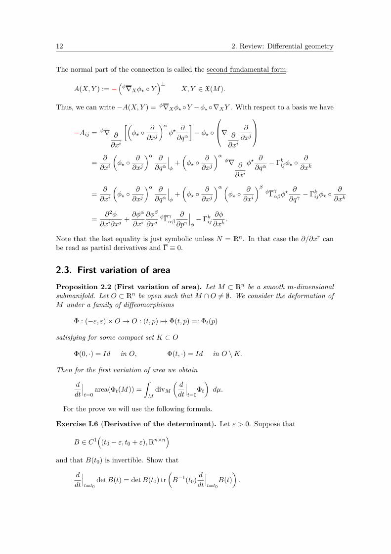
The normal part of the connection is called the second fundamental form:

A(X,Y ) := −(φ∇Xφ? Y

)⊥X,Y ∈ X(M).

Thus, we can write −A(X,Y ) = φ∇Xφ? Y −φ? ∇XY . With respect to a basis we have

−Aij = φ∇ ∂

∂xi

[(φ?

∂

∂xj

)αφ?

∂

∂qα

]− φ?

∇ ∂

∂xi

∂

∂xj

= ∂

∂xi

(φ?

∂

∂xj

)α ∂

∂qα

∣∣∣φ

+(φ?

∂

∂xj

)αφ∇ ∂

∂xi

φ?∂

∂qα− Γkijφ?

∂

∂xk

= ∂

∂xi

(φ?

∂

∂xj

)α ∂

∂qα

∣∣∣φ

+(φ?

∂

∂xj

)α (φ?

∂

∂xi

)βφΓγαβφ?

∂

∂qγ− Γkijφ?

∂

∂xk

= ∂2φ

∂xi∂xj+ ∂φα

∂xi∂φβ

∂xjφΓγαβ

∂

∂pγ

∣∣∣φ− Γkij

∂φ

∂xk.

Note that the last equality is just symbolic unless N = Rn. In that case the ∂/∂xr canbe read as partial derivatives and Γ ≡ 0.

2.3. First variation of areaProposition 2.2 (First variation of area). Let M ⊂ Rn be a smooth m-dimensionalsubmanifold. Let O ⊂ Rn be open such that M ∩O 6= ∅. We consider the deformation ofM under a family of diffeomorphisms

Φ : (−ε, ε)×O → O : (t, p) 7→ Φ(t, p) =: Φt(p)

satisfying for some compact set K ⊂ O

Φ(0, ·) = Id in O, Φ(t, ·) = Id in O \K.

Then for the first variation of area we obtain

d

dt

∣∣∣t=0

area(Φt(M)) =ˆM

divM(d

dt

∣∣∣t=0

Φt

)dµ.

For the prove we will use the following formula.

Exercise I.6 (Derivative of the determinant). Let ε > 0. Suppose that

B ∈ C1((t0 − ε, t0 + ε),Rn×n

)and that B(t0) is invertible. Show that

d

dt

∣∣∣t=t0

detB(t) = detB(t0) tr(B−1(t0) d

dt

∣∣∣t=t0

B(t)).

2.3. First variation of area 13

Proof of Proposition 2.2. The area formula tells us that

area(Φt(M)) =ˆM

Jac((Φt)?) dµ =ˆM

√det([(Φt)?]>[(Φt)?]) dµ.

Therefore, it remains to compute the derivative of the Jacobian. To simplify our compu-tation we write

Φt(p) = p+ tX(p) +O(t2), X := d

dt

∣∣∣t=0

Φt.

For the push forward of Φt we obtain

(Φt)? : TM → TRn : τk 7→ (Φt)?τk = τk + tDτkX +O(t2).

The matrix representation of (Φt)? with respect to an orthonormal basis (τi)1≤i≤m of TMand the standard basis (ej)1≤j≤n+1 of TRn+1 is given by

[(Φt)?]ij = τ ji + tDτiXj +O(t2).

Using the formula for the derivative of the determinant we can compute thatd

dt

∣∣∣t=0

√det([(Φt)?]>[(Φt)?])

= d

dt

∣∣∣t=0

√det(δij + t〈τi, DτjX〉+ t〈DτiX, τj〉+O(t2))

= 12 tr

(〈τi, DτjX〉+ 〈DτiX, τj〉

)= divM X

which proves the result.

Remark 2.3. To derive a formula for the second variation of area one can proceed in asimilar way. For the details see [56], Chapter 2.

Corollary 2.4. Let us define X := d

dt

∣∣∣t=0

Φt then

d

dt

∣∣∣t=0

area(Φt(M)) =ˆM

divM X dµ = +ˆMH〈ν,X〉 dµ+

ˆ∂M〈µ,X〉 dσ

where ν is the unit normal of M and µ is the outward unit conormal of ∂M , i.e. normalto ∂M , tangent to M and pointing away from M .Proof. Proposition 2.2 implies the first equality. To verify the second equality we choosean orthonormal frame (τi)i∈N of TM and computeˆ

MdivM X dµ =

ˆM

divM X> dµ+ˆM

divM X⊥ dµ

=ˆ∂M

⟨µ,X>

⟩dσ +

ˆM

⟨DτiX

⊥, τi⟩dµ

=ˆ∂M〈µ,X〉 dσ +

ˆMτi(⟨X⊥, τi

⟩)dµ−

ˆM

⟨(Dτiτi)

⊥ , X⟩dµ

=ˆ∂M〈µ,X〉 dσ −

ˆM

⟨〈Dτiτi, ν〉ν,X

⟩dµ


which is the desired result.

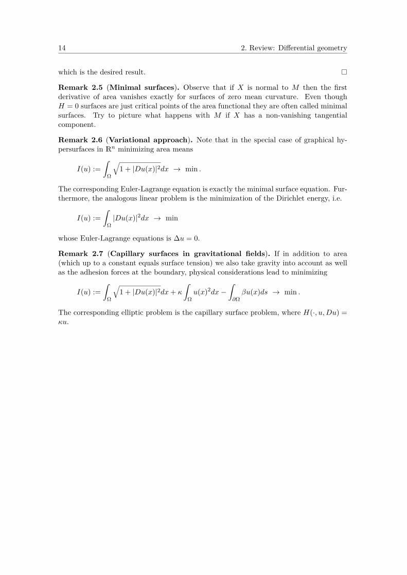
Remark 2.5 (Minimal surfaces). Observe that if X is normal to M then the firstderivative of area vanishes exactly for surfaces of zero mean curvature. Even thoughH = 0 surfaces are just critical points of the area functional they are often called minimalsurfaces. Try to picture what happens with M if X has a non-vanishing tangentialcomponent.

Remark 2.6 (Variational approach). Note that in the special case of graphical hy-persurfaces in Rn minimizing area means

I(u) :=ˆ

Ω

√1 + |Du(x)|2dx → min .

The corresponding Euler-Lagrange equation is exactly the minimal surface equation. Fur-thermore, the analogous linear problem is the minimization of the Dirichlet energy, i.e.

I(u) :=ˆ

Ω|Du(x)|2dx → min

whose Euler-Lagrange equations is ∆u = 0.

Remark 2.7 (Capillary surfaces in gravitational fields). If in addition to area(which up to a constant equals surface tension) we also take gravity into account as wellas the adhesion forces at the boundary, physical considerations lead to minimizing

I(u) :=ˆ

Ω

√1 + |Du(x)|2dx+ κ

ˆΩu(x)2dx−

ˆ∂Ωβu(x)ds → min .

The corresponding elliptic problem is the capillary surface problem, where H(·, u,Du) =κu.

3. Review: Linear PDEs of second order

3.1. Elliptic PDEs in Holder spaces

Definition 3.1 (Linear elliptic operators). Let Ω ⊂ Rn be a bounded domain andu ∈ C2(Ω). Suppose that aij , bk, c ∈ C0(Ω) and that the matrix [aij ] is symmetric. Thedifferential operator L defined by

Lu := aij(x)Diju + bk(x)Dku + c(x)u

is called elliptic in Ω if the matrix [aij(x)] is positive definite for all x in Ω. In this case

0 < λ(x) ≤ aij(x)ξiξj ≤ Λ(x) ∀ ξ ∈ Sn, ∀ x ∈ Ω (3.1)

where λ(x) and Λ(x) are the smallest and largest Eigenvalues of [aij(x)]. Furthermore, Lis called uniformly elliptic in Ω if there exist λmin and Λmax such that

0 < λmin ≤ aij(x)ξiξj ≤ Λmax <∞ ∀ ξ ∈ S, ∀ x ∈ Ω. (3.2)

Theorem 3.2 (Maximum principle). Let L be uniformly elliptic in the bounded domainΩ and c ≤ 0. Let u ∈ C2(Ω) ∩ C0(Ω). If Lu ≥ f then

supΩu ≤ sup

∂Ωu+ + c sup

Ω

(|f−|λ

).

If Lu = f then

supΩ|u| ≤ sup

∂Ω|u|+ c sup

Ω

( |f |λ

).

In both cases c = c(diam Ω, sup |b|/λ).

Proof. See [23], Theorem 3.7.

The following comparison principle is a useful consequence.

Corollary 3.3. Let Ω and L be as above. Suppose that u, v ∈ C0(Ω) ∩ C2(Ω) satisfyLu ≥ Lv in Ω and u ≤ v on ∂Ω. Then u ≤ v in Ω.

Proof. Apply Theorem 3.2 to w := u− v.

Before we can state the existence theorem for linear elliptic equations of second orderwe want to recall the definition of Holder spaces.

15

16 3. Review: Linear PDEs of second order

Definition 3.4 (Holder spaces). Let Ω ⊂ Rn be a bounded domain and 0 < α < 1. Afunction f : Ω→ R is called α-Holder continuous in x0 if

[f ]α,x0 := supx∈Ω

∣∣f(x)− f(x0)∣∣

|x− x0|α< ∞.

We say that f is uniformly α-Holder continuous in Ω if

[f ]α,Ω := supx,y∈Ωx 6=y

∣∣f(x)− f(y)∣∣

|x− y|α<∞.

The spaces

Ck,α(Ω) :=f ∈ Ck(Ω)

∣∣∣∣ Dβf unif. α-Holder cont. in Ω, ∀ β ∈ Nn, |β| = k

equipped with the norm

‖f‖Ck,α(Ω) := ‖f‖Ck(Ω) +∑|β|=k

[Dβf

]α,Ω

are Banach spaces. If α = 1 we say Lipschitz instead of 1-Holder.

Lemma 3.5. Let Ω ⊂ Rn be an open, bounded Lipschitz domain. Let k1, k2 ≥ 0 and0 ≤ α1, α2 ≤ 1. If k1 + α1 > k2 + α2 then the inclusion of Ck1,α1(Ω) into Ck2,α2(Ω) iscompact.

Proof. See [1], Section 8.6.

Now we are ready to quote a classical existence theorem for linear Dirichlet problems.

Theorem 3.6 (Existence for the linear Dirichlet problem). Let Ω ⊂ Rn be abounded C2,α-domain. Let L be an uniformly elliptic operator with coefficients in C0,α(Ω)and c ≤ 0. Furhtermore, assume that f ∈ C0,α(Ω) and φ ∈ C2,α(Ω). Then the Dirichletproblem

Lu = f in Ωu = φ on ∂Ω

has a unique solution u ∈ C2,α(Ω) satisfying

‖u‖C2,α(Ω) ≤ C(‖u‖C0(Ω) + ‖φ‖C2,α(Ω) + ‖f‖C0,α(Ω)

)where C = C

(n, α,Ω, λmin, ‖aij‖C0,α(Ω), ‖b

i‖C0,α(Ω), ‖c‖C0,α(Ω)

).

Proof. See [23], Theorem 6.6 and Theorem 6.14.

Remark 3.7. The condition c ≤ 0 is only needed for the existence and uniquenessstatement but not for the estimate. In the case that c ≤ 0 is not satisfied existence anduniqueness still hold as long as the homogeneous problem Lu = 0 in Ω, u = 0 on ∂Ω hasonly the zero solution. That is (one part of) the Fredholm alternative (see [23], Theorem6.15).

3.1. Elliptic PDEs in Holder spaces 17

If the data of the problem are more regular then also the solution possesses moreregularity.

Theorem 3.8 (Interior regularity). Let k ∈ N and Ω ⊂ Rn a bounded domain. Let Lbe a linear, uniformly elliptic operator with coefficients aij , bi, c ∈ Ck,α(Ω). Furthermore,assume that f ∈ Ck,α(Ω) and that u ∈ C2(Ω) satisfies Lu = f . Then u ∈ Ck+2,α(Ω).


Theorem 3.9 (Global regularity). Let k ∈ N and Ω ⊂ Rn a bounded Ck+2,α-domain.Let L be a linear, uniformly elliptic operator with coefficients aij , bi, c ∈ Ck,α(Ω). Fur-thermore, assume that f ∈ Ck,α(Ω) and φ ∈ Ck+2,α(Ω). If u ∈ C0(Ω) ∩ C2(Ω) satisfiesLu = f in Ω and u = φ on ∂Ω. Then u ∈ Ck+2,α(Ω).


Finally, we also want to mention the corresponding result for the oblique derivativeproblem. It includes the Neumann problem as a particular case.

Theorem 3.10 (Existence for the linear oblique Derivative problem). Let Ω ⊂ Rnbe a bounded C2,α-domain. Let L be a linear, uniformly elliptic operator with coefficientsin C0,α(Ω) and c ≤ 0. Furhtermore, assume that f ∈ C0,α(Ω) and γ, β, φ ∈ C1,α(Ω). If

γ〈β, ν〉 > 0 (ν exterior unit normal of ∂Ω)

or

〈β, ν〉 > 0, γ ≥ 0 and either c 6= 0 or γ 6= 0,

then the oblique derivative problemLu = f in Ωγu+Dβu = φ on ∂Ω

has a unique solution u ∈ C2,α(Ω) satisfying

‖u‖C2,α(Ω) ≤ C(‖u‖C0(Ω) + ‖φ‖C1,α(Ω) + ‖f‖C0,α(Ω)

)(3.3)

where

C = C(n, α,Ω, λmin, ‖aij‖C0,α(Ω), ‖b

i‖C0,α(Ω), ‖c‖C0,α(Ω),

‖γ‖C1,α(Ω), ‖βi‖C1,α(Ω), 〈β, ν〉).

Proof. See [23], Theorem 6.30, Theorem 6.31 and the following remarks about the Fred-holm alternative.

Exercise I.7 (Understanding Holder spaces). (i) Can you find a function whichis in C0,α(Ω) but not in C0,α+ε(Ω) for ε > 0? Can you find a function that is inC1,1(Ω) but not in C2(Ω)?

(ii) Can you find a domain Ω ⊂ R2 and a function u ∈ C1(Ω) which is not in C0,3/4(Ω)?

(iii) Why do we need to work with Holder spaces Ck,α(Ω) instead of the easier Ck(Ω)spaces?


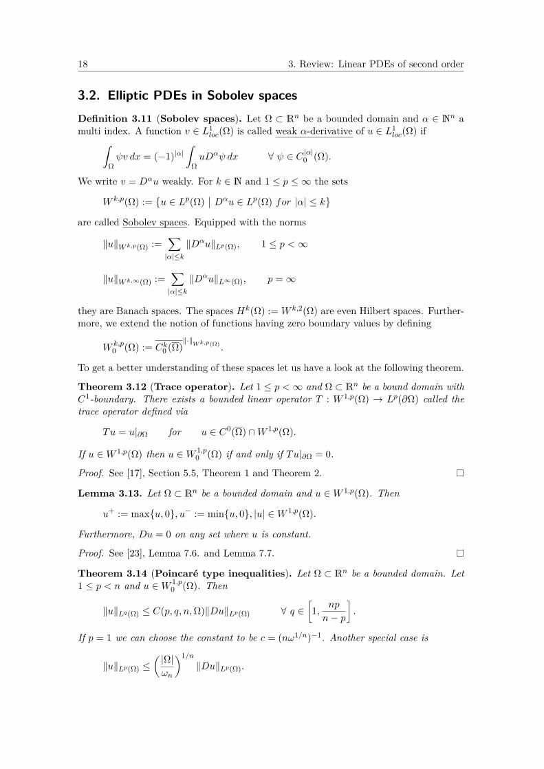
3.2. Elliptic PDEs in Sobolev spacesDefinition 3.11 (Sobolev spaces). Let Ω ⊂ Rn be a bounded domain and α ∈ Nn amulti index. A function v ∈ L1

loc(Ω) is called weak α-derivative of u ∈ L1loc(Ω) if

ˆΩψv dx = (−1)|α|

ˆΩuDαψ dx ∀ ψ ∈ C |α|0 (Ω).

We write v = Dαu weakly. For k ∈ N and 1 ≤ p ≤ ∞ the sets

W k,p(Ω) :=u ∈ Lp(Ω)

∣∣ Dαu ∈ Lp(Ω) for |α| ≤ k

are called Sobolev spaces. Equipped with the norms

‖u‖Wk,p(Ω) :=∑|α|≤k

‖Dαu‖Lp(Ω), 1 ≤ p <∞

‖u‖Wk,∞(Ω) :=∑|α|≤k

‖Dαu‖L∞(Ω), p =∞

they are Banach spaces. The spaces Hk(Ω) := W k,2(Ω) are even Hilbert spaces. Further-more, we extend the notion of functions having zero boundary values by defining

W k,p0 (Ω) := Ck0 (Ω)

‖·‖Wk,p(Ω) .

To get a better understanding of these spaces let us have a look at the following theorem.

Theorem 3.12 (Trace operator). Let 1 ≤ p <∞ and Ω ⊂ Rn be a bound domain withC1-boundary. There exists a bounded linear operator T : W 1,p(Ω) → Lp(∂Ω) called thetrace operator defined via

Tu = u|∂Ω for u ∈ C0(Ω) ∩W 1,p(Ω).

If u ∈W 1,p(Ω) then u ∈W 1,p0 (Ω) if and only if Tu|∂Ω = 0.

Proof. See [17], Section 5.5, Theorem 1 and Theorem 2.

Lemma 3.13. Let Ω ⊂ Rn be a bounded domain and u ∈W 1,p(Ω). Then

u+ := maxu, 0, u− := minu, 0, |u| ∈W 1,p(Ω).

Furthermore, Du = 0 on any set where u is constant.

Proof. See [23], Lemma 7.6. and Lemma 7.7.

Theorem 3.14 (Poincare type inequalities). Let Ω ⊂ Rn be a bounded domain. Let1 ≤ p < n and u ∈W 1,p

0 (Ω). Then

‖u‖Lq(Ω) ≤ C(p, q, n,Ω)‖Du‖Lp(Ω) ∀ q ∈[1, np

n− p

].

If p = 1 we can choose the constant to be c = (nω1/n)−1. Another special case is

‖u‖Lp(Ω) ≤( |Ω|ωn

)1/n‖Du‖Lp(Ω).

3.2. Elliptic PDEs in Sobolev spaces 19

Proof. See [17], Section 5.6, Theorem 3 and [23], inequality (7.44).

An important relation between the Holder spaces and the Sobolev spaces is given by(one of) the Sobolev embedding theorem(s).

Theorem 3.15 (Sobolev embedding theorem). Let Ω ⊂ Rn be a bounded domainwith Lipschitz boundary. Let p ∈ [1,∞) and u ∈W k,p(Ω). If

0 ≤ m < k − n

p< m+ 1

then u ∈ Cm,k−np−m(Ω). For smaller Holder coefficients the embedding is even compact.

Note that the regularity assumption for ∂Ω can be dropped if we consider the space W k,p0 (Ω)

instead.

Proof. See for example [23], Chapter 7, Theorem 7.26 or [17], Chapter 5, Section 6,Theorem 6.

Theorem 3.16 (Morrey’s estimate). Let u ∈W 1,1(Ω). If there exists some α ∈ (0, 1)and K > 0 such thatˆ

BR

|Du|dx ≤ KRn−1+α, ∀ BR ⊂ Ω

Then u ∈ C0,α(Ω) with [Du]α,Ω ≤ c(n, α,K). If Ω = Ω ∩ xn > 0 for some domainΩ ⊂ Rn and the above inequality holds for all BR ⊂ Ω then u ∈ C0,α(Ω ∩ Ω).


Remark 3.17. The last part of the theorem will be particularly useful for local estimatesnear a flattened boundary.

Next we want to recall the Holder continuity of weak solutions.

Definition 3.18 (Weak solutions). Let Ω ⊂ Rn be a bounded domain. We considerthe linear operator

Lu := Di(aijDju) + bkDku+ cu

with coefficients aij , bk, c ∈ C0(Ω) and such that [aij ] satisfies (3.2). Let g, f i ∈ L1(Ω). Ifu ∈W 1,2(Ω) satisfies

ˆΩ

[(aijDju− f i

)Djξ −

(bkDku+ cu− g

)ξ]

= 0 ∀ ξ ∈ C10 (Ω)

we say that u is a weak solution of Lu = g +Difi.

Remark 3.19. Note that weak solutions can be defined for more general operators andunder weaker conditions on the coefficients. Note also that the integral equality remainstrue for test functions ξ ∈W 1,2

0 (Ω).

Theorem 3.20 (Maximum principle). Let Ω ⊂ Rn be a bounded domain and L as inDefinition 3.18. Let u ∈ C0(Ω) ∩W 1,2(Ω) satisfy Lu ≥ 0 in a weak sense. If c ≤ 0 then

supΩu ≤ sup

∂Ωu+.



Theorem 3.21 (Interior Holder continuity). Let Ω ⊂ Rn be a bounded domain. Letf i ∈ Lq(Ω) for some q > n. Let u ∈ W 1,2(Ω) be a weak solutionf of Di(aijDju) = Dif

i

in Ω. Then

‖u‖C0,α(Ω′) ≤ c(n, q, d,Λmax/λmin)(‖u‖L2(Ω) + λ−1

min‖f‖Lq(Ω))

where Ω′ ⊂⊂ Ω, d = dist(Ω′, ∂Ω) and α = α(n,Λmax/λmin).


Theorem 3.22 (Boundary Holder continuity). Let Ω ⊂ Rn be a domain satisfyinga uniform exterior cone condition with cones V on a boundary portion T . Let f i ∈ Lq(Ω)for some q > n. Let u ∈W 1,2(Ω) be a weak solution of Di(aijDju) = Dif

i in Ω. If thereexits K,α0 > 0 such that

osc∂Ω∩BR(x0)

u ≤ KRα0 ∀ x0 ∈ T,R > 0.

Then

‖u‖C0,α(Ω′) ≤ c(n, q, d, α0, V,Λmax/λmin)(‖u‖C0(Ω) +K + λ−1

min‖f‖Lq(Ω)).

Here Ω′ ⊂⊂ Ω ∪ T , d = dist(Ω′, ∂Ω \ T ) and α = α(n, q, α0, V,Λmax/λmin).


For the sake of completeness let us also mention the existence result in the weak setting.

Theorem 3.23 (Weak existence). Suppose that Ω ⊂ Rn satisfies an exterior conecondition on all points of ∂Ω. Let φ ∈ C0(∂Ω) and f i ∈ Lq(Ω) for some q > n.Then thereexists a unique weak solution u ∈W 1,2

loc (Ω) of Di(aijDju) = Difi satisfying u = φ on ∂Ω.


3.3. Parabolic PDEs in Holder spacesDefinition 3.24 (Parabolic Holder spaces). Let Ω ⊂ Rn be a bounded domain andT > 0. We set QT := Ω × (0, T ), ST := ∂Ω × (0, T ) and start with a definition of theparabolic analogue of the spaces Ck(Ω):

Ck;b k2 c(QT ) :=

f : QT → R∣∣∣ ‖u‖

Ck;b k2 c(QT ):=

k∑i=0

∑|γx|+2|γt|=i

supQT

|Dγtt D

γxx f | <∞

Let us denote the Holder coefficients of a function f : QT → R by

[f ]x,α,QT := sup(x,t),(y,t)∈QT

x 6=y

|f(y, t)− f(x, t)||y − x|α

3.3. Parabolic PDEs in Holder spaces 21

and

[f ]t,α,QT := sup(x,s),(x,t)∈QT

s6=t

|f(x, t)− f(x, s)||t− s|α

.

The parabolic Holder spaces are defined as

Ck,α;b k2 c,α2 (QT ) :=

u ∈ Ck,b

k2 c(QT )

∣∣∣ ‖u‖Ck,α;b k2 c,

α2 (QT )

<∞

with

‖u‖Ck,α;b k2 c,

α2 (QT )

:= ‖u‖Ck;b k2 c(QT )

+∑

2|γt|+|γx|=k[Dγt

t Dγxx u]x,α,QT +

∑0<k+α−2|γt|−|γx|<2

[Dγtt D

γxx u]t,β,QT

where 2β := k + α− 2|γt| − |γx|.

Exercise I.8. What are the components of the ‖ · ‖C2,α;1, α2 (QT )-norm?

Definition 3.25 (Linear uniformly parabolic differential operators). Let aij , bk, c ∈C0(QT ) and suppose that [aij ] is symmetric. Let u ∈ C2,1(QT ). The operator ∂/∂t − Ldefined by

∂u

∂t− Lu := ∂u

∂t− aijDiju+ bkDku+ cu

is called parabolic. It is called uniformly parabolic in QT if additionally

0 < λmin ≤ aij(x, t)ξiξj ≤ Λmax <∞

holds for all (x, t) ∈ QT and all ξ ∈ S.

Theorem 3.26 (Existence for the parabolic Dirichlet boundary value problem).Let Ω ⊂ Rn be a bounded domain with C2,α-boundary and T > 0. Let ∂/∂t − L beuniformly parabolic in QT . Suppose that aij , bk, c, f ∈ C0,α,0,α2 (QT ), φ ∈ C2,α,1,α2 (ST ) andu0 ∈ C2,α(Ω). If the compatibility conditions

φ(·, 0) = u0,∂

∂t

∣∣∣t=0

φ = aij(·, 0)Diju0 − bk(·, 0)Dku0 − c(·, 0)u0 + f(·, 0)

are satisfied on ∂Ω. Then the problem

∂u

∂t− Lu = f in Ω× (0, T )

u = φ on ∂Ω× (0, T )

u(·, 0) = u0 on Ω× 0

has a unique solution u ∈ C2,α,1,α2 (QT ) which satisfies

‖u‖C2,α;1, α2 (QT ) ≤ C

(‖f‖

C0,α;0, α2 (QT ) + ‖φ‖C2,α;1, α2 (ST ) + ‖u0‖C2,α(Ω)

).

If the coefficients and right hand sides are more regular the solution will be more regulartoo. However, to obtain more regular solutions up to t = 0 one also has to impose higherorder compatibility conditions.


Proof. See [38], Chapter 5, Theorem 5.2.

Theorem 3.27 (Existence for the parabolic Neumann boundary value prob-lem). Let Ω ⊂ Rn be a bounded domain with C2,α-boundary and T > 0. Let ∂/∂t −L be uniformly parabolic in QT . Suppose that aij , bk, c, f ∈ C0,α,0,α2 (QT ), βk, γ, φ ∈C1,α;0,α2 (ST ) and u0 ∈ C2,α(Ω). If the compatibility condition

φ(·, 0) = βk(·, 0)Dku0 + γ(·, 0)u0 on ∂Ω

is satisfied and the transversality condition holds, i.e. for the outward unit normal µ of∂Ω× (0, T ) we have

〈β, µ〉 > 0 on ∂Ω× (0, T ).

Then the problem

∂u

∂t− Lu = f in Ω× (0, T )

βkDku+ γu = φ on ∂Ω× (0, T )

u(·, 0) = u0 on Ω× 0

(3.4)

has a unique solution u ∈ C2,α,1,α2 (QT ) which satisfies

‖u‖C2,α;1, α2 (QT ) ≤ C

(‖f‖

C0,α;0, α2 (QT ) + ‖φ‖C1,α;0, α2 (ST ) + ‖u0‖C2,α(Ω)

).

If the coefficients and right hand sides are more regular the solution will be more regulartoo. However, to obtain more regular solutions up to t = 0 one also has to impose higherorder compatibility conditions.

Proof. See [38], Chapter 5, Theorem 5.3.

Remark 3.28 (Differentiable functions defined on hypersurfaces/ boundaries).As in the differential geometry section we say that a function is in Ck(S) for some Ck-hypersurface S ⊂ Rn if the composition with a chart has that regularity as a map froman open subset of Rn into R. Let k ≥ 0 and a domain Ω ⊂ Rn with Ck-boundary. Ifφ ∈ Ck(Ω) then φ

∣∣∂Ω defines a function in Ck(∂Ω). Conversely, if φ ∈ Ck(∂Ω) then there

exists φ ∈ Ck(Ω) such that both functions agree on the boundary and have equivalentnorms. The same result carries over to the parabolic setting and to Holder norms wherethe norms are compute in charts and the global norm is defined via a partition of unity.That is how we understand terms like ‖φ‖

C2,α;1, α2 (ST ).

Remark 3.29 (PDEs on manifolds). In the situation where Ω ⊂ Rn is replaced bya smooth Riemannian manifold (Mn, g) we have to modify the definition of the norms.They can defined locally via charts and globally via a partition of unity. Note that in thiscontext the norms depend on the choice of atlas. Once this is done, one obtains the sameexistence results for the linear Dirichlet and Neumann problem as above. Furthermore,one could allow a time dependent metric g(·, t).

The most important tool for second order parabolic equations is the maximum principle.Before we mention it we define sub- and supersolutions.

3.3. Parabolic PDEs in Holder spaces 23

Definition 3.30 (Super- and subsolutions). Let v+, v− ∈ C2,1(Ω× (0, T )) ∩ C0(Ω×[0, T ]). We say that v+ is a supersolutions of (3.4) if it satisfies

∂v+

∂t− Lv+ ≥ f1 in Ω× (0, T )

Nv+ := βkDkv+ + γv+ ≥ f2 on ∂Ω× (0, T )

v+ ≥ u0 on Ω× 0.

The function v− is called subsolution if the opposite inequalities hold.

Now we can state the version of the maximum principles which we use in this work.

Theorem 3.31 (Parabolic maximum principle). Let u ∈ C0(Ω × [0, T ]) ∩ C2,1(Ω ×(0, T )) be a solution of (3.4). Assume that L and N have bounded coefficients, that ∂/∂t−Lis uniformly parabolic and that the Neumann condition is oblique. If v+ and v− are super-and subsolutions of (3.4) then v− ≤ u ≤ v+ in QT .

Proof. Note that for w := v+−u and w := u−v− we have ∂w/∂t−Lw ≥ 0, Nw ≥ 0 andw( . , 0) ≥ 0. So we can reduce the proof to the case of the upper bound for f1 = 0, f2 = 0and u0 = 0. This proof is contained in [53] Chapter 3, Section 3, Theorem 5,6 and 7.Furthermore Stahl proved in [57] the generalization which in particular allows for themore general operator N which occurs here.

Corollary 3.32. If f1 ≡ 0 and f2 ≡ 0, then v+ := maxΩ u0 is a supersolution if

cmaxΩ

u0 ≥ 0 and γmaxΩ

u0 ≥ 0.

Furthermore v− := minΩ u0 is a subsolution if

cminΩu0 ≤ 0 and γmin

Ωu0 ≤ 0.

Obviously, these inequalities are all satisfied for c ≡ 0 and γ ≡ 0.

Corollary 3.33 (Comparison to the ODE). Assume that f1 ≡ 0, f2 ≡ 0, γ = 0 andc(x, t) = c(t). Then v+ given as a solution of

(ODE)

∂v+

∂t+ cv+ ≥ 0 on Ω× (0, T )

v+(0) = maxΩ

u0

is a supersolution. Furthermore, the function v− satisfying the same ODE with the reverseinequality and the initial value minΩ u0 is a subsolution.

Part II.

Nonlinear elliptic PDEs of secondorder

25

4. General theory for quasilinear problems

4.1. Fixed point theorems: From Brouwer to Leray-Schauder

We start by recalling Brouwer’s fixed point theorem.

Theorem 4.1 (Brouwer). Let us denote by B the closed ball Br(x0) ⊂ Rn of radius rcentered at x0. If f : B → B is continuous then f has a fixed point.

Idea of proof. Suppose that f : Br(x0) → Br(x0) has no fixed point. Then x and f(x)always span a line. Therefore, we can define a map

R : Br(x0)→ ∂Br(x0) : x 7→ Rx

where Rx is given as the point of intersection between the line segment starting from f(x)in direction x and ∂Br(x0). Note that R is a retraction, i.e. R is continuous and satisfiesRx = x for all x in ∂Br(x0). If we regard the set of points in Br(x0) as a membrane.Then the map R describes a continuous deformation of such a membrane which movesall points to the boundary. Intuitively, the membrane will be torn apart.

For a proof of the non-existence of such a retraction we refer to literature, e.g. [67],Section 1.14 or [55], Section 1.2. The proof also occurred as an exercise on homeworksheet four in Michael Eichmair’s class Differential Geometry II from last semester.

This result can be extended to compact, convex subsets of a Banach space.

Theorem 4.2 (Schauder). Let (X, ‖ · ‖) be a Banach space and A ⊂ X compact andconvex. If T : A→ A is continuous then T has a fixed point.

Proof. Since A is compact for every k ∈ N we find a finite number N ∈ N of points xi ∈ Asuch that

A ⊂N⋃i=1

B1/k(xi), N = N(k), xi = xi(k).

Let us denote the convex hull of xi | 1 ≤ k ≤ N by Acok . Note that Acok ⊂ A. We definethe continuous map

Jk : A→ Acok : x 7→ Jk(x) :=∑Ni=1 dist

(x,A \B1/k(xi)

)xi∑N

i=1 dist(x,A \B1/k(xi)

) .Since Acok is convex and generated by a finite number of elements it is homeomorphic viaa map h to a closed ball B in some Euclidean space. From Brouwer’s Theorem 4.1 wesee that h (Jk T ) h−1 : B → B has a fixed point and thus the same holds for Jk Trestricted to Acok .

27

28 4. General theory for quasilinear problems

We denote the sequence of fixed points of Jk T by (x(k))k∈N. Note that A is compact.Therefore, there exists a subsequence (x(kl))l∈N which converges to some x ∈ A as kltends to infinity. We observe that∣∣∣Tx− x∣∣∣ = lim

l→∞

∣∣∣Tx(kl) − x(kl)∣∣∣ = lim

l→∞

∣∣∣Tx(kl) − (T Jkl)(x(kl))

∣∣∣ ≤ liml→∞

1kl

= 0.

Thus, x is a fixed point of T .

Corollary 4.3. Let (X, ‖ · ‖) be a Banach space and A ⊂ X closed and convex. IfT : A→ A is continuous and TA is relativly compact then T has a fixed point.

Exercise II.1. Try to prove Corolloary 4.3. Hint: Ist the set (TA)co compact?

Based on Corollary 4.3 we obtain the version which is important for our application.

Theorem 4.4 (Schaefer). Let (X, ‖ · ‖) be a Banach space and T : X → X continuousand compact. If

M =x ∈ X

∣∣ ∃σ ∈ [0, 1] : x = σTx

is bounded then T has a fixed point.

Proof. Let M be strictly bounded by M > 0. Define the map T ∗ : BM (0)→ BM (0) by

T ∗x :=

Tx for ‖Tx‖X ≤M,

M

‖Tx‖XTx for ‖Tx‖X > M.

Note that T ∗ is continuous and BM (0) is closed and convex. Since T is compact TBM (0)is relatively compact. Thus, also T ∗BM (0) is relatively compact and by Corollary 4.3 T ∗has a fixed point x∗. Now, suppose that ‖Tx∗‖X > M . On the one hand

x∗ = T ∗x∗ = M

‖Tx∗‖XTx∗

yields ‖x∗‖X = M . On the other hand x∗ = σTx∗ (σ = M/‖Tx∗‖X) implies ‖x∗‖X < M .Therefore, ‖Tx∗‖X ≤M and x∗ = T ∗x∗ = Tx∗.

One can even allow a more general dependence on the paramenter σ.

Theorem 4.5 (Leray-Schauder). Let (X, ‖·‖) be a Banach space and T : X×[0, 1]→ Xcontinuous and compact. If T (·, 0) = 0 and

M =x ∈ X

∣∣ ∃σ ∈ [0, 1] : x = T (x, σ)

is bounded then T (·, 1) has a fixed point.

Proof. For our purpose the theorem of Schaefer will be sufficient. Therefore, we skip theproof and refer for it to [23], Theorem 11.6.

4.2. Reduction to a priori estimates in the C1,β-norm 29

4.2. Reduction to a priori estimates in the C1,β-normWe consider the following family of quasilinear Dirichlet problems of second order

(DP)σ

Qσu := aij(·, u,Du)Diju+ σb(·, u,Du) = 0 in Ω,

u = σφ on ∂Ω

with σ ∈ [0, 1], continuous coefficients aij , b ∈ C0(Ω × R × Rn) and symmetric matrix[aij ]. Furthermore, we set Q := Q1 and (DP) := (DP)1.

Definition 4.6. Let A ⊂ Rn. The operator Q is called elliptic in A if [aij(x, z, p)] ispositive definite for all (x, z, p) ∈ A × R × Rn. Furthermore, Q is called elliptic w.r.t.v ∈ C1(A) if [aij(x, v(x), Dv(x))] is positive definite for all x ∈ A.

Let T be the operator which assignes to v the solution u of the linear problem

aij(·, v,Dv)Diju+ b(·, v,Dv) = 0 in Ω, u = φ on ∂Ω. (4.1)

We see that the existence of a fixed point of T guarantees the existence of a solution of(DP). Based on this observation Theorem 4.4 yields a first criterion for existence.

Theorem 4.7 (Existence criterion: C1,β-version). Let Ω ⊂ Rn be a bounded domainwith C2,α-boundary. Let Q be elliptic in Ω with coefficients aij , b ∈ C0,α(Ω×R×Rn) andφ ∈ C2,α(Ω) for some α ∈ (0, 1). If there exists some β ∈ (0, 1) such that the set

u ∈ C2,α(Ω)∣∣ ∃ σ ∈ [0, 1] : u solves (DP)σ

is bounded in C1,β(Ω) independently of σ. Then (DP) has a solution in C2,α(Ω).

Proof. Let v ∈ C1,α(Ω). Then (4.1) is a linear, uniformly elliptic problem for u withcoefficients in C0,αβ(Ω). By Theorem 3.6 there exists a unique solution u ∈ C2,αβ(Ω) ⊂C1,β(Ω). Thus, the operator

T : C1,β(Ω)→ C1,β(Ω) : v 7→ Tv := u,

is well defined. We need to show that T has a fixed point. By Theorem 4.4 this follows if Tis a continuous, compact operator and the setM = u ∈ C1,β(Ω) | ∃σ ∈ [0, 1] : u = σTuis bounded. The latter is true by assumption1 so it remains to verify continuity andcompactness.

Compactness: By Theorem 3.6 we have

‖Tv‖C2,αβ(Ω) ≤ c(‖Tv‖C0(Ω) + ‖φ‖C2,αβ(Ω) + ‖|b(·, v,Dv)‖C0,αβ(Ω)

)with c = c

(n, α,Ω, ‖aij(·, v,Dv)‖C0,αβ(Ω),minΩ λ(·, v,Dv)

)and from Theorem 3.2 we

obtain the C0 estimate

‖Tv‖C0(Ω) ≤ ‖φ‖C0(Ω) + c(diam Ω)∥∥∥∥ b(·, v,Dv)λ(·, v,Dv)

∥∥∥∥C0(Ω)

.

1Note that v ∈ M ⇒ v = σTv ∈ C2,αβ(Ω) ⇒ v = σTv ∈ C2,α(Ω).


Therefore, we see that T maps bounded subsets of C1,β(Ω) into bounded subsets ofC2,αβ(Ω) which by Arzela-Ascoli are relatively compact in C1,β(Ω), i.e. T is compact.

Continuity: Suppose that vmm∈N ⊂ C1,β(Ω) converges in the C1,β-norm to somev. In particular this sequence is bounded in the C1,β-norm. As above this implies thatTvmm∈N is bounded in the C2,αβ-norm. Thus by Arzela-Ascoli Tvmm∈N is relativelycompact in C2(Ω). This is equivalent to the existence of a subsequence Tvmkk∈N whichconverges in the C2(Ω)-norm to some u ∈ C2(Ω). Since aij and b are continuous thisyields

0 = limk→∞

(aij(x, vmk(x), Dvmk(x))Dij(Tvmk(x)) + b(x, vmk(x), Dvmk(x))

)

= aij(x, v(x), Dv(x))Diju(x) + b(x, v(x), Dv(x)) ∀ x ∈ Ω.

This shows that Tv = u. Finally, all subsequences have to converge to the same limitwhich shows that T is continuous.

4.3. Reduction to a priori estimates in the C1-norm

The previous result shows that the existence proof is reduced to a priori estimates inC1,β(Ω). It turns out that the Holder estimate for Du can be carried out under very mildassumptions on the operator Q. This will help us to then formulate an existence criterionbased on C1 a priori estimates.

Theorem 4.8. Let Ω ⊂ Rn be a bounded domain with C2-boundary. Let Q be elliptic inΩ with coefficients aij ∈ C1(Ω × R × Rn), b ∈ C0(Ω × R × Rn) and let φ ∈ C2(Ω). Ifu ∈ C2(Ω) solves (DP) then there exists β ∈ (0, 1) such that

[Du]β,Ω ≤ C

(n, Ω, K, minUK λ, ‖a

ij‖C1(UK), ‖b‖C0(UK), ‖φ‖C2(Ω)

)<∞

with K := ‖u‖C1(Ω) and UK := Ω× [−K,K]× [−K,K]n.

Remark 4.9. The result was first obtained independently by De Giorgi and Nash forlinear operators in divergence form: Lu = Di(aij(x)Dju). It was a major break throughin the study of nonlinear elliptic PDEs. Later Morrey and Stampachia extended the workto linear elliptic operators of general form. The theorem as it is stated above goes backto Ladyzhenskaya and Ural’ceva.

Proof. The proof can be found in [23], Theorem 13.7. For our later application to theprescribed mean curvature equation it will be enough to consider operators in divergenceform, i.e. a ∈ C1(Ω×R×Rn,Rn), b ∈ C0(Ω×R×Rn,R):

div a(·, u,Du) + b(·, u,Du) = 0. (4.2)

In that case the proof is contained in [23], Theorem 13.1 (interior estimate) and Theorem13.2 (boundary estimate). We will only give a sketch of these arguments here.

4.3. Reduction to a priori estimates in the C1-norm 31

Interior estimate: Multiplying (4.2) by a test function ξ ∈ C10 (Ω), integrating over Ω

and doing an integration by parts on the first term yieldsˆ

Ω

[ai(·, u,Du)Diξ − b(·, u,Du)ξ

]dx = 0.

We put ξ := Dkη and perform an integration by parts on the first term w.r.t. Dk:ˆ

Ω

[(∂ai

∂xk+ ∂ai

∂zDku+ ∂ai

∂pjDkju

)Diη + bDkη

]dx = 0

where all partial derivatives of ai and b are evaluated at (x, u(x), Du(x)). Thus we getˆ

Ω

(aij(x)Djw + f i

)Diη dx = 0

with w := Dku and

aij(x) := ∂ai

∂pj(x, u(x), Du(x)),

f i(x) :=(∂ai

∂xk+ pk

∂ai

∂z+ δikb

)(x, u(x), Du(x)).

So w is a weak solution of the linear, uniformly elliptic equation Di(aij(x)Djw) = −Difi

with bounded coefficients and Theorem 3.21 yields the interior estimate.

Boundary estimate: W.l.o.g. we may assume φ ≡ 0 (or consider u − φ instead of u).Let x0 ∈ ∂Ω. Choose a small ball B(x0) and a C2-diffeomorphism ψ which flattens outthe boundary locally near x0, i.e. such that

D+ := ψ(B(x0) ∩ Ω) ⊂ Rn−1 × [0,∞), ∂0D+ := ψ(B(x0) ∩ ∂Ω) ⊂ Rn−1 × 0.

In the new coordinates y = ψ(x) the function v := (u ψ−1) satisfies again an equationof the form

div a(·, v,Dv) + b(·, v,Dv) = 0 (4.3)

which implies that w := Dykv is a weak solution of a linear equation Di(aijDjw) = −Difi

where the derivatives are taken w.r.t. y now. Let 1 ≤ k ≤ n− 1: Since we assumed thatu = 0 on ∂Ω we have u ψ−1 = 0 on ∂0D

+ and thus w = 0 on ∂0D+. By Theorem 3.22

this implies a Holder estimate for w in D′ ∩D+ for any D′ ⊂⊂ D.Note that we can not apply this strategy to get the estimate for w = Dnv since we have

no information about Dnv on the boundary. Instead we try to verify thatˆBR(y0)∩D+

|Dw|2dy ≤ cRn−2+2α, w = Dnv (4.4)

for y0 ∈ D′ ∩D+ and R > 0 sufficiently small such that B2R(y0) ⊂ D. Using the Holderinequality ‖u‖L1(BR) ≤ cRn/2‖u‖L2(BR) and the Morrey estimate, Theorem 3.16, we willthen obtain the desired Holder estimate. In order to prove (4.4) we solve equation (4.3)


for Dnnv: Dnnv = CjkDjkv +C with 1 ≤ k ≤ n− 1. This shows that it suffices to verify(4.4) for w = Dkv and 1 ≤ k ≤ n− 1. So we put w = Dkv and choose η = ρ2(w− c) withc = w(y0) if B2R(y0) ⊂ D+ and zero otherwise. Plugging this into (4.3) yields

0 =ˆD+

[ρ2aijDiwDjw + 2ρaijDiρDjw(w − c) + ρ2f iDiw + 2ρ(w − c)f iDiρ

]dx.

Now we choose ρ ∈ C1c (B2R(y); [0, 1]) such that ρ ≡ 1 on Br(y). Furthermore, we use the

ellipticity of [aij ] and Young’s inequality ab ≤ εa2/2 + b2/2ε to compute

λ

ˆBR(y0)∩D+

|Dw|2 dx ≤ˆB2R(y0)

ρ2aijDiwDjw dy

≤ˆB2R(y0)∩D+

(c1|Dρ||Dw||w − c|+ c2|Dw|+ c3|w − c||Dρ|

)dy

≤ c4

ˆB2R(y0)∩D+

(1 + |Dρ|2|w − c|2 + (ε2

1 + ε22)|Dw|2

)dy.

Choosing ε1 and ε2 small enough, e.g. (ε21 + ε2

2) ≤ λ/2, we can absorb the last terminto the right hand side. Using the Holder continuity of w and choosing ρ such that|Dρ| ≤ 2/R we obtain

ˆBR(y0)∩D+

|Dw|2 ≤ c5

(Rn +Rn−2 sup

B2R(y0)∩D+|w − c|2

)≤ c6R

n−2+2α.

This yields the Morrey estimate for w = Dkv and as explained above also for Dnv. Finally,we rewrite the estimate in terms of u and repeat it in a finite number of balls which cover∂Ω. This yields the desired result.

Together with Theorem 4.7 this improves our existence criterion.

Corollary 4.10 (Existence criterion: C1-version). Let Ω ⊂ Rn be a bounded domainwith C2,α-boundary. Let Q be elliptic in Ω with coefficients aij ∈ C1(Ω × R × Rn),b ∈ C0,α(Ω×R×Rn) and φ ∈ C2,α(Ω) for some α ∈ (0, 1). If the set

u ∈ C2,α(Ω)∣∣ ∃ σ ∈ [0, 1] : u solves (DP)σ

is bounded in C1(Ω) independently of σ. Then (DP) has a solution in C2,α(Ω).

5. The prescribed mean curvature problem

In the following we are interested in Dirichlet problem for the prescribed mean curvatureequation (PMC) := (PMC)1 where

(PMC)σ

div

(Du√

1 + |Du|2

)− σH(·, u,Du) = 0 in Ω

u = σφ on ∂Ω

for a given function H.

5.1. C0-estimateLet us first derive a comparison principle for quasilinear equations. It will be useful forthe proof of the C0-estimate as well as for the proof of the boundary gradient estimate.

Theorem 5.1 (Comparison principle for quasilinear elliptic PDEs). Let Ω ⊂ Rnbe a bounded domain and u, v ∈ C2(Ω). Suppose that Q is a quasilinear operator withcontinuous coefficients such that

(a) Q is uniformely elliptic with respect to u or v,(b) aij is independent of z,(c) b is non-increasing in z,(d) aij and b are continuously differentiable in p.

If Qu ≥ Qv in Ω and u ≤ v on ∂Ω then u ≤ v in Ω. If Qu > Qv in Ω then the weakerassumptions (a)− (c) yield the stronger conclusion u < v in Ω.

Proof. Let Q be elliptic w.r.t. u. We put w := u − v and us := su + (1 − s)v. Using(b), (c) and (d) we compute on the set where w > 0:

0 ≤ Qu−Qv

= aij(·, Du)Dij(u− v) +[aij(·, Du)− aij(·, Dv)

]Dijv

+[b(·, u,Du)− b(·, u,Dv)

]+[b(·, u,Dv)− b(·, v,Dv)

]≤ aij(·, Du)Dij(u− v) +

[(ˆ 1

0

∂aij

∂pk

∣∣∣(·,Dus)

dsDijv

)+(ˆ 1

0

∂b

∂pk

∣∣∣(·,u,Dus)

ds

)]Dkw

=: aijDijw + bkDkw =: Lw.

We see that Lw ≥ 0 in w > 0 and w ≤ 0 on ∂Ω. Therefore, w = 0 on ∂w > 0 andwe can use (a) and apply the linear maximum principle, Theorem 3.2 to conclude that

33

34 5. The prescribed mean curvature problem

w ≤ 0 in w > 0. Thus w = u− v ≤ 0 in Ω. If we have a strict inequality, at a criticalpoint we have Du = Dv and thus

0 < aijDijw

even without computing the partial derivatives w.r.t. pk. Therefore, w can not have anonnegative maximum in Ω, i.e. w = u − v < 0 in Ω. Finally, if Q is uniformly ellipticw.r.t v then we obtain the reverse inequalities and apply the minimum principle.

Remark 5.2. The Theorem can be relaxed to allow u ∈ C0(Ω)∩C2(Ω). In this situationthe uniform ellipticity in (a) is replace by locally uniform ellipticity. This is important ifone tries to derive existence results for C0 boundary data.

This works because the corresponding linear result, Theorem 3.2 does not actuallyrequire uniform ellipticity but only ellipticity together with demanding bk/[akk] to belocally bounded. Furthermore, it can be extended to hold for u ∈ C1(Ω)∩W 2,n(Ω)∩C0(Ω).

Corollary 5.3 (Uniqueness). Let Ω ⊂ Rn be a bounded domain. Let φ ∈ C0(Ω).Suppose that the operator Q satisfies the conditions of Theorem 5.1. Then there is atmost one solution u ∈ C0(Ω) ∩ C2(Ω) satisfying Qu = 0 in Ω and u = φ on ∂Ω.

Proof. Clear.

Proposition 5.4. Let Ω ⊂ Rn. Let u ∈ C0(Ω) ∩ C2(Ω) be a solution of (PMC)σ. If

supΩ×R×Rn

|H| ≤ n

RΩ, RΩ := diam Ω

2

and H is non-decreasing in z. Then the following estimate holds

supΩ|u| ≤ sup

Ω|φ|+RΩ.

Proof. Exercise. Hint: Use the comparison principle Theorem 5.1 and compare the solu-tion to spherical caps, i.e. the graphs of the functions

v± : BRΩ(x0)→ R : x 7→ v±(x) := ±(

supΩ|φ|+

√R2

Ω − |x− x0|2)

for some x0 ∈ Rn such that Ω ⊆ BRΩ(x0).

The following theorem provides another tool to prove a priori estimates for generalquasilinear elliptic operators:

Theorem 5.5. Let Q be a quasilinear operator which is elliptic in Ω ⊂ Rn. Let g ∈Lnloc(Rn) and h ∈ Ln(Ω) be non-negative functions which satisfyˆ

Ωhn ≤

ˆRngn.

Let u ∈ C0(Ω) ∩ C2(Ω) be a solution of Qu := aij(·, u,Du)Diju+ b(·, u,Du) = 0. If

b(x, z, p)sgn(z)n(det[aij(x, z, p)])1/n ≤

h(x)g(p) ∀ (x, z, p) ∈ Ω×R×Rn

then u satisfies the estimate

supΩ|u| ≤ sup

∂Ω|u|+ c(g, h) diam(Ω).

5.1. C0-estimate 35

Proof. A proof can be found in [23], Theorem 10.5.

Exercise II.2. Use Theorem 5.5 to prove C0-a priori estimates for solutions of (PMC).Which condition do you have to impose on the right hand side, i.e. on H?

Remark 5.6. In general, Theorems which provide estimates for a broad class of (non-linear) equations will not provide optimal results. However, they are useful to get a firstintuition for the conditions which might be needed. Better results can be expected frommethods which make use of the special structure of the equation. Following this strat-egy we skip the proof of Theorem 5.5 and focus instead on a C0-a priori estimate whichincoorporates the special structure of the (PMC) problem.

First, we will prove an estimate in Lnn−1 which we wil then turn into a C0-estimate

using Stampacchia’s lemma.

Proposition 5.7. Let Ω ⊂ Rn be a bounded domain with C1-boundary and φ ∈ C0(∂Ω).Let u ∈ C2(Ω) ∩ C0(Ω) be a solution of (PMC)σ for some σ ∈ [0, 1] and H ∈ C0,1(Ω ×R×Rn) such that H is increasing in z. If there exists ε ∈ (0, 1] such that∣∣∣∣ ˆ

ΩH(·, 0, Dη)η dx

∣∣∣∣ ≤ (1− ε)ˆ

Ω|Dη| dx ∀ η ∈ C1

0 (Ω) (5.1)

Then uk := maxu− k, 0 and uk := max−u− k, 0 satisfy

‖uk‖L

nn−1 (Ω)

≤ | spt uk|nεω

1/nn

, ‖uk‖L

nn−1 (Ω)

≤ | spt uk|nεω

1/nn

for all k ≥ k0 := sup∂Ω |φ|.

Proof. Using Theorem 3.12 and Lemma 3.13 we see that uk ∈ W 1,20 (Ω). Therefore, we

can use uk as a test function in the weak formulation of div a− σH = 0. Note that

p · a(p) = |p|2√1 + |p|2

≥ |p| − 1. (5.2)

We put A(k) := spt uk and estimate

‖Duk‖L1(Ω) − |A(k)| =Â(k)

(|Duk| − 1

)dx

(5.2)≤Â(k)

Diuk · ai(Duk) dx

=Â(k)

Diuk · ai(Du) dx =Â(k)−σH(·, u,Du)uk dx ≤

Â(k)−σH(·, 0, Du)uk dx

≤∣∣∣∣ ˆ

ΩH(·, 0, Duk)uk dx

∣∣∣∣ (5.1)≤ (1− ε)

ˆΩ|Duk| dx = (1− ε)‖Duk‖L1(Ω).

Finally, we use the Poincare type inequality from Theorem 3.14 to obtain

‖uk‖L

nn−1 (Ω)

≤ 1nω

1/nn

‖Duk‖L1(Ω) ≤|A(k)|nεω

1/nn

.

The second estimate follows by considering uk in A(k) := spt uk.


In the next step we present the Lemma of Stampacchia [60].Lemma 5.8 (Stampacchia). Let ψ : [k0,∞)→ [0,∞) be decreasing, γ > 1 and supposethat

(h− k)ψ(h) ≤ c[ψ(k)

]γ ∀ h > k ≥ k0.

Then for

d := 2γγ−1 c[ψ(k0)

]γ−1

we have ψ(k0 + d) = 0.Proof. Let us put ki := k0 + d − d

2i . We apply the inequality with h = ki+1 and k = kiand get

ψ(ki+1) ≤ 2i+1c

d

[ψ(ki)

]γ.

We will show by induction that

ψ(ki) ≤ψ(k0)

2i/(γ−1) .

For i = 0 this is clear. Suppose this is true for i. Then

ψ(ki+1) ≤ 2i+1c

d

[ψ(ki)

]γ ≤ 2i+1c

d

[ψ(k0)

]γ2iγ/(γ−1) = ψ(k0)

2(i+1)/(γ−1)

which finishes the induction and shows that limi→∞

ψ(ki) = 0. Thus, taking the limit ofψ(ki) ≥ ψ(k0 + d) ≥ 0 as i→∞ yields the result.

Theorem 5.9 (C0-estimate). Let Ω ⊂ Rn be a bounded domain with C1-boundary andφ ∈ C0(∂Ω). Let u ∈ C2(Ω) ∩ C0(Ω) a solution of (PMC)σ for some σ ∈ [0, 1] andH ∈ C0,1(Ω×R×Rn) increasing in z. If there exists an ε ∈ (0, 1] such (5.1) holds. Thenwe obtain the following C0-estimate

supΩ|u| ≤ sup

∂Ω|φ| + 2n+1

nε0

( |Ω|ωn

)1/n.

Proof. Let uk := maxu − k, 0 for k ≥ k0 := sup∂Ω |φ| and A(k) := spt uk. UsingProposition 5.7 we obtain for h > k

(h− k)|A(h)| ≤Â(h)

(u− k) dx ≤Â(k)

uk dx

≤ |A(k)|1/n‖uk‖L

nn−1 (Ω)

≤ 1nεω

1/nn

|A(k)|1+1/n.

Now we set ψ(k) := |A(k)| and apply Stampacchia’s Lemma 5.8 with γ = 1 + 1/n

∣∣x ∈ Ω | u(x) > d+ k0∣∣ = 0 for d := 2n+1

nε

( |A(k0)|ωn

)1/n.

Since u is continuous this implies

supΩu ≤ sup

∂Ω|φ| + 2n+1

nε

( |Ω|ωn

)1/n.

Similarly we can estimate −u using uk := max−u − k, 0 and ψ(k) := | spt uk|. Thisyields the desired result.

5.2. Interior gradient estimate 37

5.2. Interior gradient estimateAs for the C0-estimate, one can derive theorems which yield an interior gradient estimate(in terms of the gradient at the boundary) for general quasilinear elliptic equations. Seefor example [23], Theorem 15.2 which implies a result for (PMC) in the case H = H(x)or Theorem 15.6 for equations in divergence form.

The idea is to differentiate the PDE w.r.t. Dk to multiply by Dku and to sum overk. This yields a PDE for |Du|2. If that PDE satisfies the assumptions of the maximumprinciple one obtains and estimate for |Du|. We will follow this approach for (PMC): Letus use the following definitions

ai(Du) := Diu√1 + |Du|2

aij(Du) := ∂ai

∂pj

∣∣∣Du

= 1√1 + |Du|2

(δij − DiuDju

1 + |Du|2

)

Hxk := ∂H

∂xk, Hz := ∂H

∂z, Hpk := ∂H

∂pk

v :=√

1 + |Du|2.

Let us assume that u ∈ C3(Ω). Then we can compute

0 = (Dku)Dk

(Dia

i −H)

= (Dku)Di

(aijDjku

)− (Dku)

(Hxk +HzDku+HplDklu

)= Di

(aijDkuDjku

)− aijDk

i uDkju− 〈Du,Hx〉 −Hz|Du|2 −HplDkuDklu.

Note that aijDikuDkj u ≥ 0. Therefore, we obtain for w := |Du|2/2:

Lw := Di(aijDjw)−HplDlw ≥ −|Hx||Du|+Hz|Du|2

in the case that H = H(z, p) with Hz ≥ 0 we get Lw ≥ 0 and the maximum principleTheorem 3.20 is applicable. The same remains true when we replace H by σH. So weobtain the following result.

Proposition 5.10 (Interior gradient estimate: H = H(z, p)). Let Ω ⊂ Rn be abounded domain. Let u ∈ C2,α(Ω) be a solution of (PMC)σ with σ ∈ [0, 1] and u ∈[−m,M ]. Assume that for some β ∈ (0, 1) we have

H ∈ C1,β([−m,M ]×Rn), Hz ≥ 0.

Then the estimate

supΩ|Du| ≤ sup

∂Ω|Du|

holds.


Proof. The proof is contained in the computation above. the higher regularity of u followsfrom the fact that H ∈ C1,β([−m,M ]×Rn) together with the regularity result for linearequations, Theorem 3.8.

To treat functions which also depend on x we need to modify the function w to com-pensate for bad terms of lower order. We make use of the following relations.

Lemma 5.11. Using the definitions above we have the following relations

aijDiuDju = v−3|Du|2, aijDiuDjv = v−4DkwDku

aijDikuDkj u ≥ 0, Di(aijDju) = v−2

(H − 2v−3DkuDkw

).

Proof. Exercise.

Proposition 5.12 (Interior gradient estimate: H = H(x, z)). Let Ω ⊂ Rn be abounded domain. Let u ∈ C2,α(Ω) be a solution of (PMC)σ with σ ∈ [0, 1] and u ∈[−m,M ]. Assume that for some β ∈ (0, 1)

H ∈ C1,β(Ω× [−m,M ]), Hz ≥ 0.

Then the estimate

supΩ|Du| ≤ c(1 + sup

∂Ω|Du|)

holds for some c = c(m + M, supΩ×[−m,M ] |H|, supΩ×[−m,M ] |Hx|). If H ≥ 0 then theconstant does not depend on |H|.

Proof. W.l.o.g. we only consider the subdomain where |Du| > 1. We set v :=√

1 + |Du|2,w := log v + f(u) and assume that f ′ ≥ 0. Using Lemma 5.11 we compute

Lw := Di(aijDjw) + bkDkw

:= Di

(aij[v−2Djw + f ′Dju

])+ 2v−1aikDiv

[v−2Dkw + f ′Dku

]= v−2Di(aijDjw) + f ′Di(aijDju) + f ′′aijDiuDju+ 2v−1f ′aikDivDku

≥ −v−2|Hx||Du|+ f ′v−2(H − 2v−3DkuDkw

)+ f ′′v−3|Du|2 + 2v−1f ′aikDivDku

≥ v−3(f ′′|Du|2 − v|Du||Hx| − v|f ′||H|

).

Let us first discuss the case m = 0. Using f(z) := exp(µz) we see that

Lw ≥ v−3|Du|2(f ′′ − 2|H|f ′ − 2|Hx|

)= v−3|Du|2eµu

(µ2 − 2|H|µ− 2|Hx|

)≥ 0

for µ := 2(|H|+ |Hx|+1). Thus, the maximum principle, Theorem 3.20 yields an estimatefor w which implies

supΩ|Du| ≤ sup

Ωexp(w − f(u))

≤ exp(

ln sup∂Ω

√1 + |Du|2 + 2 exp(µM)

)≤ (1 + sup

∂Ω|Du|2) exp(2 exp(µM)).

5.2. Interior gradient estimate 39

To deal with arbitrary values of m we note that u := u+m ≥ 0 satisfies

div(

Du√1 + |Du|2

)= H(x, u−m) in Ω.

Therefore, the argument above yields an estimate for |Du| = |Du| with M replaced byM +m.

Remark 5.13. The same argument yields an interior gradient estimate for H = H(x, z, r)where r stands for a |Du|2 dependence. In this case we have to assume Hz ≥ 0 andHr ≤ 0. However, note that in this case the boundedness of |H| and |Hx| which appearin the constant is not guaranteed for arbitrary H. So we could not allow for H =f(x, u)

√1 + |Du|2 even if we impose the conditions f ≤ 0 and fz ≥ 0 (which imply

Hz ≥ 0 and Hr ≤ 0) because the quantities H and Hx are not bounded.

An extension of the previous proposition to a more geometric dependence on Du iscontained in the following theorem.

Theorem 5.14 (Interior gradient estimate: H = H(x, z, ν)). Let Ω ⊂ Rn be abounded domain. Let u ∈ C2,α(Ω) be a solution of (PMC)σ with σ ∈ [0, 1] and u ∈[−m,M ]. Assume that for some β ∈ (0, 1)

H ∈ C1,β(Ω× [−m,M ]×Rn+1), H = H(x, u, ν(Du)), Hz ≥ 0.

Then the estimate

supΩ|Du| ≤ c

(1 + sup

∂Ω|Du|

)

holds for some c = c(n,m + M, sup |H|, sup |Hx|, sup |Hν |) where the supremum is takenover Ω× [−m,M ]× Sn+1.

Proof. Exercise.

Exercise II.3 (Interior gradient estimate: H = H(x, z, ν)). Prove the interior gra-dient estimate, Theorem 5.14. Hint: Use the ansatz w := log v + f(u) and computeLw := ∆M w where ∆M is the Laplace Beltrami operator on M = graph u.

Remark 5.15. The interior estimates we proved shift the problem from the interior tothe boundary. So we see that the estimate finally relies on a boundary gradient estimate.One can also prove a purely interior estimate of the kind

|Du(0)| ≤ c exp(

1 + M2

r2

), u ∈ C3(Br(0)).

That is done for example for (PMC) in [64] on just two pages. The advantage is that suchan estimate can also be used for solutions u ∈ C2(Ω) ∩C0(Ω). This permits to prove theexistence for less regular boundary data φ ∈ C0(∂Ω).


5.3. Boundary gradient estimate

The last quantity which remains to be estimated is the gradient of the solution u of(PMC)σ at the boundary. For that purpose we use barriers. The idea of barriers is tofind functions w± which have the same boundary values φ and lie above and below thesolution u. Thus, the gradient of u can be estimates with the help of the gradients of w±.We start with a general definition of barriers.

Definition 5.16 (Definition of Barriers). Let Ω ⊂ Rn be a bounded domain and letthe quasilinear operator Q satisfy the conditions of the comparison principle, Theorem5.1. Let d0 > 0 and d := dist(·, ∂Ω). We define the boundary strip

Γ0 :=x ∈ Ω | d(x) < d0

.

Let u ∈ C0(Ω) ∩ C2(Ω) be a solution of

Qu = 0 in Ω, u = φ on ∂Ω. (5.3)

If there are functions w± ∈ C2(Γ0) such that

(i) w− = u = w+ on ∂Ω,

(ii) w− ≤ u ≤ w+ on ∂Γ0 ∩ Ω,

(iii) Qw+ < 0 < Qw− in Γ0 ∩ Ω

holds. Then w± are called upper and lower barriers for solutions u of (5.3) in Γ0.

Remark 5.17. At first, one could think that it is easier to require that (ii) holds inΓ0 and to ignore (iii). However, since the solution u is unknown it is not clear how toconstruct w± which satisfy (ii) in all of Γ0 but also (i). Whereas on ∂Γ0 ∩Ω this can berealized by demanding w+ ≥M and w− ≤ −m where u ∈ [−m,M ].

The next lemma shows that (ii) and (iii) together with the comparison principle implythe validity of (ii) in all of Γ0.

Lemma 5.18 (Application of Barriers). Let Ω ⊂ Rn be a bounded domain withC2-boundary. Let Q be a quasilinear elliptic Operator satisfying properties (a) − (c) ofTheorem 5.1 and φ ∈ C2(Ω). Furthermore, let d0 > 0 be sufficiently small such thatd ∈ C2(Γ0) and that ‖u− φ‖C0(Γ0) ≤ 1. Let ψ satisfy

ψ ∈ C2([0, d0]), ψ(0) = 0, ψ(d0) ≥ 1. (5.4)

If the functions w± := ±ψ d +φ satisfy ±Qw± ≤ 0 in Γ0 ∩ Ω. Then they are barriersfor a solution u ∈ C2(Ω) of (5.3) in Γ0 and the estimate

sup∂Ω|Du| ≤ |ψ′(0)|+ sup

∂Ω|Dφ|

holds.

5.3. Boundary gradient estimate 41

Proof. Due to the choice of d0 > 0 we see that w± ∈ C2(Γ0). Next we observe thatψ(0) = 0 implies (i) and ψ(d0) ≥ 1 ≥ ‖u− φ‖C0(Γ) implies (ii). Therefore, we have

w− ≤ u ≤ w+ on ∂Γ0. (5.5)

Now we apply the comparison principle to Q in Γ0 ∩ Ω. By condition (iii) of Definition5.16 and the assumptions on Q, Theorem 5.1 implies that (5.5) holds in Γ0. Thus,

|Du| ≤ |Dw±| ≤ |ψ′(0)D d |+ |Dφ|.

Since |D d | = 1 the result follows.

It turns out that the mean curvature of ∂Ω will play a role. We use the followingconvention.

Definition 5.19 (Mean curvature of ∂Ω). Let Ω ⊂ Rn be a bounded domain withC2-boundary. At y ∈ ∂Ω we can choose a coordinate system such that e1, . . . , en−1 aretangent to ∂Ω and en is the inward pointing unit normal of ∂Ω. Locally, the boundarycan be described as the graph of a C2-function f in these coordinates. We define

H∂Ω(y) := ∆f∣∣y

which is the mean curvature of graph f with respect to the lower unit normal to the graph,i.e. the outward pointing unit normal of ∂Ω.

We will make use of a relation between the mean curvature of the boundary and thedistance function.

Lemma 5.20. Let Ω ⊂ Rn be a bounded domain with C2-boundary. Then there existssome d0 > 0 such that d := dist(·, ∂Ω) ∈ C2(Γ0). Furthermore, for x ∈ Γ0 and y ∈ ∂Ωsuch that d(x) = |x− y| we have

[D2 d(x)] = diag

[ −κ1(y)1− κ1(y) d(x) , · · · ,

−κn−1(y)1− κn−1(y) d(x) , 0

],

provided we choose a coordinate system centered at y with basis vectors pointing in theprincipal directions. Here κi(y) are the principal curvatures of ∂Ω in y and κi(y) ≤ d−1

0 .In particular,

∆ d(x) = −n−1∑i=1

κi(y)1− κi(y) d(x) ≤ −

n−1∑i=1

κi(y) = −H∂Ω(y).

Proof. Exercise. A proof can be found in [23], Lemma 14.16 and Lemma 14.17.

Exercise II.4. Try to prove Lemma 5.20. In particular, verify that

∆ dist(x, ∂Ω) ≤ −H∂Ω(y)

where y ∈ ∂Ω is such that dist(x, ∂Ω) = |x− y|.

Let us first consider the case H = 0, i.e. minimal surfaces.


Proposition 5.21 (Boundary gradient estimate: H ≡ 0). Let Ω be a bounded domainwith C2-boundary. Let φ ∈ C2(Ω). If u ∈ C2(Ω) satisfies (PMC)σ with H ≡ 0, i.e. theminimal surface equation and the mean curvature of ∂Ω is non-negative, i.e. H∂Ω ≥ 0.Then the following a priori estimate holds

sup∂Ω|Du| ≤ c

(d0, ‖ d ‖C2(Γ0), ‖φ‖C2(Γ0)

).

Proof. Let us choose d0 > 0 sufficiently small (as in Lemma 5.18) and make the ansatzw± = ±ψ d +φ. We consider the equivalent operator

Qu := aij(Du)Diju :=((1 + |Du|2)δij −DiuDju

)Diju = 0.

We need to show that ±Qw± ≤ 0 for a function ψ satisfying (5.4). We start by computing

Diw± = ±ψ′Di d +Diφ (5.6)

|Dw±|2 = (ψ′)2 ± 2ψ′〈D d, Dφ〉+ |Dφ|2 ≤ (ψ′ + |Dφ|)2 (5.7)

Dijw± = ±ψ′′Di dDj d±ψ′Dij d +Dijφ. (5.8)

We obtain three terms which will be estimated separately:

±Qw± = ψ′aij(Dw±)Dij d +ψ′′aij(Dw±)Di dDj d±aij(Dw±)Dijφ.

Since |D d | = 1 we see that Di dDij d = 0. Together with Lemma 5.20 we obtain

ψ′aij(Dw±)Dij d

= ψ′(1 + |Dw±|2)∆ d−ψ′DiφDjφDij d

≤ −ψ′(1 + |Dw±|2)H∂Ω(y) + c1(‖φ‖C1(Γ0), ‖d ‖C2(Γ0)

)(ψ′)2

where we assumed that ψ′ ≥ 1. To estimate the second term we assume ψ′′ ≤ 0. Sinceaij is positive definite we could ignore this term but it will be needed to compensate badterms. So we compute

ψ′′(d)aij(Dw±)Di dDj d

= ψ′′((1 + |Dw±|2)|D d |2 − 〈Dw±, D d〉2

)= ψ′′

(1 + (ψ′)2 ± 2ψ′〈D d, Dφ〉+ |Dφ|2 − (ψ′ ± 〈D d, Dφ〉)2

)= ψ′′

(1 + |Dφ|2 − 〈D d, Dφ〉2

)≤ ψ′′.

The third term can be estimated by

±aij(Dw±)Dijφ ≤ c2(‖φ‖C2(Γ0)

)(1 + |Dw±|2) ≤ c2

(‖φ‖C2(Γ0)

)(ψ′)2

5.3. Boundary gradient estimate 43

where we assumed once more that ψ′ ≥ 1. In total we obtain

±Qw± ≤ −(1 + |Dw±|2)ψ′H∂Ω + (c1 + c2)(ψ′)2 + ψ′′. (5.9)

Let a, b > 0. We choose ψ(d) := a log(1 + bd). Note that ψ(0) = 0 and ψ′′ = −a−1(ψ′)2 ≤0. Since H∂Ω ≥ 0 we obtain

±Qw± ≤ (c1 + c2)(ψ′)2 − a−1(ψ′)2 < 0

provided a−1 ≥ c1 + c2. Furthermore, we need to verify ψ(d0) ≥ 1 and ψ′(d) ≥ 1. Alltogether we need to check that:

a log(1 + bd1) ≥ 1, ab

1 + bd1≥ 1, a−1 ≥ c1 + c2.

where d1 ∈ (0, d0). All this can be achieved for

a := 1c1 + c2 + 1 , d1 := mind0, a/2, b := max

1

a− d1,exp(a−1)− 1

d1

and from Lemma 5.18 we obtain the estimate

sup∂Ω|Du| ≤ ab+ sup

∂Ω|Dφ| ≤ c

(d0, ‖d ‖C2(Γ0), ‖φ‖C2(Γ0)

).

Remark 5.22. Note that the condition H∂Ω ≥ 0 was needed here because the |Dw±|2term is of order (ψ′)2 so in total the first term is of order (ψ′)3 and we can not absorb itinto the good term ψ′′ which is only of order (ψ′)2. Later we will see that the conditionon the mean curvature of ∂Ω is sharp.

In the next step we extend our barrier construction to the situation where H = H(x, u).

Proposition 5.23 (Boundary gradient estimate: H = H(x, z)). Let Ω be a boundeddomain with C2-boundary and φ ∈ C2(Ω). Let u ∈ C2(Ω) be a solution of (PMC)σ. IfH ∈ C1(Γ0× [−R,R]) for R := 1+supΓ0 |φ| and satisfies Hz ≥ 0 and the Serrin condition

H∂Ω(y) ≥ |H(y, φ(y))| ∀ y ∈ ∂Ω. (5.10)

Then the following a priori estimate holds

sup∂Ω|Du| ≤ c

(d0, ‖d ‖C2(Γ0), ‖φ‖C2(Γ0), ‖H‖C1(Γ0×[−R,R])

).

Proof. Let us choose d0 > 0 sufficiently small (as in Lemma 5.18). We make the ansatzw± = ±ψ d +φ and consider the equivalent operator

Qσu := aij(Du)Diju− b(·, u)

:=((1 + |Du|2)δij −DiuDju

)Diju− σ(1 + |Du|2)3/2H(·, u).


We need to show that ±Qw± ≤ 0 for a function ψ satisfying (5.4). Recall the formulaefor w±, i.e. (5.6) and our result for aij(Du)Diju. in (5.9). We obtain

±Qw± = ±aij(Dw±)Dijw± ∓ σ(1 + |Dw±|2)3/2H(·, w±)

≤ −(1 + |Dw±|2)ψ′H∂Ω(y) + c(ψ′)2 + ψ′′ ∓ σ(1 + |Dw±|2)3/2H(·, w±)

= −(1 + |Dw±|2)ψ′(H∂Ω(y)± σH(·, w±)

)+ c(ψ′)2 + ψ′′

∓ σ(1 + |Dw±|2)(√

1 + |Dw±|2 − ψ′)H(·, w±).

Before we continue we note that

H∂Ω(y)± σH(x,w±(x))

= H∂Ω(y)± σH(y, φ(y))∓ σ[H(y, φ(y))−H(x, φ(y))

]∓ σ

[H(x, φ(y))−H(x, φ(x))

]∓ σ

[H(x, φ(x))−H(x,±ψ d(x) + φ(x))

].

The last ∓[. . .]-term is always positive since ψ d ≥ 0 and Hz ≥ 0. Together with its prefactor −(1 + |Dw±|2)ψ′ it is negative so we can drop it. Using ψ′(d) ≥ 1 we have

1 + |Dw±|2 ≤ c (|Dφ|) (ψ′)2,∣∣∣√1 + |Dw±|2 − ψ′

∣∣∣ ≤ 1 + |Dφ|.

Using the Serrin condition and assuming |ψ d| ≤ 1 we obtain

±Qw±

≤ −(1 + |Dw±|2)ψ′(H∂Ω(y)± σH(y, φ(y))

)+ c(ψ′)2 + ψ′′

+ (1 + |Dw±|2)ψ′(∣∣∣H(y, φ(y))−H(x, φ(y))

∣∣∣+ ∣∣∣H(x, φ(y))−H(x, φ(x))∣∣∣)

+ (1 + |Dw±|2)∣∣∣√1 + |Dw±|2 − ψ′

∣∣∣|H(·, w±)|

≤ c(ψ′)2 + ψ′′ + (1 + |Dw±|2)ψ′(

supΓ0×[−R,R]

|Hx|+ supΓ0×[−R,R]

|Hz| supΓ0

|Dφ|)

d

+ (1 + |Dw±|2)(1 + |Dφ|) supΓ0×[−R,R]

|H|

≤ c(1 + ψ′ d)(ψ′)2 + ψ′′.

We choose ψ(d) := a log(1 + bd). Note that ψ(0) = 0 and ψ′′ = −a−1(ψ′)2 ≤ 0. Thus

±Qw± ≤ c(1 + ψ′ d)(ψ′)2 − a−1(ψ′)2 ≤ 0

provided ψ′(d) d ≤ 1 and a−1 ≥ 2c. Furthermore, we need to verify ψ(d0) ≥ 1 andψ′(d) ≥ 1. All together we need to check that:

a log(1 + bd) ≥ 1, abd

1 + bd≤ 1, ab

1 + bd≥ 1, a−1 ≥ 2c.

5.4. Existence and uniqueness theorem 45

where d1 ∈ (0, d0). All this can be achieved for

a := 12c+ 1 , d1 := mind0, a/2, b := max

1

a− d1,exp(a−1)− 1

d1

and from Lemma 5.18 we obtain the estimate

sup∂Ω|Du| ≤ ab+ sup

∂Ω|Dφ| ≤ c

(d0, ‖d ‖C2(Γ0), ‖φ‖C2(Γ0), ‖H‖C1(Γ0×[−R,R])

)where R := 1 + supΓ0 |φ|. Note that we used |w±| ≤ |ψ d |+ |φ| ≤ R in Γ0.

As for the interior gradient estimate one can extend the result to right hand sides whichdepend on the unit normal of the graph, i.e.

H = H(x, u, ν(Du)), ν(Du) := 1√1 + |Du|2

(−Du

1

).

Theorem 5.24 (Boundary gradient estimate: H = H(x, z, ν)). Let Ω be a boundeddomain with C2-boundary and φ ∈ C2(Ω). Let u ∈ C2(Ω) be a solution of (PMC)σ. LetH ∈ C1(Γ0 × [−R,R]×Rn+1) for R := 1 + supΓ0 |φ|, H = H(x, z, ν). If satisfies Hz ≥ 0and the generalized Serrin condition

H∂Ω(y) ≥∣∣∣∣∣H(y, φ(y),

(±µ(y)

0

))∣∣∣∣∣ ∀ y ∈ ∂Ω. (5.11)

Then the following a priori estimate holds

sup∂Ω|Du| ≤ c

(d0, ‖ d ‖C2(Γ0), ‖φ‖C2(Γ0), ‖H‖C1(Γ0×[−R,R]×[−1,1]n+1)

).

Proof. Exercise.

Exercise II.5. Try to prove Theorem 5.24, i.e. a boundary gradient estimate in the casewhere H = H(x, z, ν). Hint: Try a proof along the lines of the proof of Theorem 5.23.Show first that∣∣∣∣∣H(x, φ(x), ν(Dw±)

)−H

(y, φ(y),

(±µ(y)

0

))∣∣∣∣∣ ≤ c1 d(x) + c2ψ′(d(x)) .

where y ∈ ∂Ω is such that d(x) = |x− y|.

5.4. Existence and uniqueness theoremBefore we state the existence theorem let us remark that no additional assumption isneeded for the C0-estimate for surfaces of constant mean curvature (CMC).

Proposition 5.25 (C0-estimate for CMC surfaces). Let Ω ⊂ Rn be a bounded domainwith C2,α boundary. Let u ∈ C2(Ω) be a solution of (PMC) with constant right hand sideH ∈ R and boundary value φ ∈ C2(Ω). If H∂Ω ≥ |H| then the estimate

supΩ|u| ≤ sup

∂Ω|φ|+ ediam(Ω)(1+|H|)

holds.


Proof. We make the ansatz

v : Ω→ R : x 7→ sup∂Ω|φ|+ eµδ

µ

(1− e−µ d(x)

), µ := 1 + |H|, δ := diam(Ω).

Using H∂Ω ≥ |H| together with Lemma 5.20 we obtain

∆ d ≤ −H∂Ω ≤ −|H|.

This estimate is valid on the subset Ω1 ⊂ Ω consisting of points having a unique closestpoint on ∂Ω. On Ω1 we compute

aijDijv :=((1 + |Dv|2)δij −DivDjv

)Dijv = |Dv|

[(1 + |Dv|2)∆ d−µ

]≤ −|Dv|

[(1 + |Dv|2)|H|+ 1 + |H|

]≤ −|Dv|(2 + |Dv|2)|H|

≤ −(1 + |Dv|2)3/2|H| ≤ (1 + |Dv|2)3/2H.

Thus

Qv := aijDijv − (1 + |Dv|2)3/2H ≤ 0 = Qu in Ω1.

From the proof the the quasilinear comparison principle we see that this allows us toconstruct a linear operator L such that L(u − v) ≥ 0 in Ω1. Therefore, the maximumprinciple for linear operators implies that the maximum of u− v is attained on ∂Ω or inΩ \ Ω1.

Let us assume that the maximum is attained at a point x ∈ Ω \ Ω1. Let y ∈ ∂Ω be aclosest point to x on ∂Ω. We put γ : [0, 1]→ R : t 7→ γ(t) := ty + (1− t)x. If w = u− vhas a maximum at x then

d+

dt

∣∣∣t=0

(w γ)(t) = 〈Du(x), y − x〉 − eµ(δ−d)d+

dt

∣∣∣t=0

(d γ)(t) ≤ 0.

Therefore, we must have Du(x) 6= 0. On the other hand, starting from x the function vis monotone decreasing along γ. This shows that if w has a maximum at x also u = v+wmust have a maximum at x and therefore Du(x) = 0. This contradiction shows that themaximum must be attained on ∂Ω.

Finally, we can put together all a priori estimates in order to obtain an existence resultfor (PMC).

Theorem 5.26 (Existence and Uniqueness for (PMC)). Let n ≥ 2, Ω ⊂ Rn bea bounded domain with C2,α-boundary and φ ∈ C2,α(Ω) for some α ∈ (0, 1). Let H ∈C1,β(Ω×R×Rn+1), H = H(x, u, ν(Du)).Suppose that H satisfies Hz ≥ 0 and

H∂Ω(y) ≥∣∣∣∣∣H(y, φ(y),

(±µ(y)

0

))∣∣∣∣∣ ∀ y ∈ ∂Ω. (5.12)

If H is not constant assume also that for some ε > 0∣∣∣∣ ˆΩH(·, 0, ν(Dη))η dx

∣∣∣∣ ≤ (1− ε)ˆ

Ω|Dη| dx ∀ η ∈ C1

0 (Ω). (5.13)

Then the Dirichlet problem of prescribed mean curvature (PMC) has a unique solutionu ∈ C2,α(Ω).

5.4. Existence and uniqueness theorem 47

Proof. All conditions of Corollary 4.10 are satisfied. Therefore, the existence proof isreduced to a priori estimates in C1(Ω) for solutions u ∈ C2,α(Ω) of (PMC)σ. IfH = const.the boundedness of |u| follows from Proposition 5.25. Otherwise, this bound follows from(5.13) together with Theorem 5.9. The gradient can be estimated in the interior with thehelp of Theorem 5.14. Finally, the boundary gradient estimate is guaranteed by (5.12)and Theorem 5.24. Uniqueness follows from Corollary 5.3 together with Hz ≥ 0.

Remark 5.27 (Sharpness of the Serrin condition). Inequality (5.12) is called Serrincondition. It is sharp in the following sense: If H ∈ C1(Ω) is either non-positive ornon-negative and

H∂Ω(y) < |H(y)| for some y ∈ ∂Ω.

Then for any δ > 0 there exists some φ ∈ C∞(Ω) with supΩ |φ| < δ such that (PMC)has no solution. See [23], Corollary 14.13 and (14.86). For the minimal surface equation,i.e. H ≡ 0 this yields solvability for all φ ∈ C2,α(Ω) if and only if H∂Ω ≥ 0, i.e. in meanconvex domains.

Remark 5.28. The dependence of H on the gradient via the normal was first investigatedby Bergner [4] who obtained a result in convex domains. The boundary gradient estimatevia the generalized Serrin condition (which also allows non-convex domains) was obtainedby the author [42] in his diploma thesis under the supervision of Gerhard Huisken.

6. General theory for fully nonlinearproblems

The main tool in the existence proof will be a Banach space version of the inverse functiontheorem. In order to state it we recall the following definition.

Definition 6.1 (Differentiability in normed spaces). Let X,Y and Z be normedspaces and X ⊂ X open. A map T : X → Z is called Gateaux-differentiable at x0 ∈ X ifthere exists a bounded linear map Lx0 ∈ L(X,Z) such that

limt→0

T (x0 + tx)− T (x0)t

= Lx0x ∀ x ∈ X.

T is called Frechet-differentiable at x0 ∈ X if the convergence is uniform in x ∈ BX , i.e.

‖T (x0 + x)− T (x0)− Lx0(x)‖Z‖x‖X

→ 0, as ‖x‖X → 0.

T is called Gateaux- (or Frechet)-differentiable in X if the corresponding statement holdsfor all x0 ∈ X. We use the classical notation

DT : X → L(X,Z) : x 7→ DT∣∣x

:= Lx

The map x 7→ Lx is denoted by DT .Suppose that T : X × Y → Z is Gateaux- (or Frechet)-differentiable at (x0, y0). Then

the partial Gateaux- (or Frechet)-derivatives are bounded linear maps L1(x0,y0) : X → Z

and L2(x0,y0) : Y → Z such that

L(x0,y0)(x, y) = L1(x0,y0)(x) + L2

(x0,y0)(y).

Here we use the notation D1T or DxT and similarly D2T or DyT .

Remark 6.2. The Frechet derivative is the generalization of the total derivative of a mapT : U ⊂ Rn → Rm. The Gateaux derivative is the analogue of the directional derivative.Note that we have the classical properties (linearity, chain rule, etc.). In particular, if Tis Gateaux-differentiable and DT ) is continuous, then T is Frechet-differentiable, moreprecisely continuously Frechet-differentiable.

Let us now state a version of the inverse function theorem in Banach spaces.

Theorem 6.3 (Inverse function theorem for Banach spaces). Let X,Z be Ba-nach spaces and X ⊂ X be open. Suppose that T : X × R → Z is continuouslyFrechet-differentiable at (x0, σ0) with T (x0, σ0) = 0 and that the partial Frechet-derivativeD1T

∣∣(x0,σ0) is invertible1. Then there exists ε > 0 such that for all σ ∈ (σ0 − ε, σ0 + ε)

there exists xσ ∈ X with T (xσ, σ) = 0.1Since X and Y are Banach spaces and L := D1T

∣∣(x0,σ0)

∈ L(X,Z) the bijectivity of L implies alreadythat L is an isomorphism, i.e. that L−1 is continuous. This follows from the open mapping theorem.

49

50 6. General theory for fully nonlinear problems

Proof. See, [23], Theorem 17.6.

Remark 6.4 (Nash-Moser inverse function theorem). In some problems it mighthappen that one loses regularity, i.e. that the solutions of a second order problem havenot necessarily two degrees of regularity more than the right hand side. In this situationone can not use the inverse function theorem in the Banach space setting. However, thereis a version by Nash and Moser (explained in detail by Hamilton [26]) which allows usto replace the Banach spaces by C∞. Nash used this tool first in [49] for his theorem onisometric embeddings. Later the result was applied by Hamilton in [27] to give a firstprove of the well-posedness of Ricci flow2.

6.1. Fully nonlinear Dirichlet problemsDefinition 6.5 (Nonlinear Dirichlet problem). Let Ω ⊂ Rn be a bounded domain.We denote by Sym(Rn) the space of symmetric real valued matrices and consider thecontinuous map

F : Γ := Ω×R×Rn × Sym(Rn)→ R : (x, z, p, q) 7→ F (x, z, p, q).

Assume that F is differentiable. Then we put

Fqij := ∂F

∂qij, Fpk := ∂F

∂pk, Fz := ∂F

∂z

and use the short cut [u] := (·, u,Du,D2u). We say that F is elliptic in A ⊂ Γ if thematrix [Fqij ] is positive definite in A. Furthermore, F is called uniformly elliptic in A if

0 < λmin ≤ Fqijξiξj ≤ Λmax <∞ ∀ ξ ∈ Sn

Finally, F is called (uniformly) elliptic with respect to u ∈ C2(Ω) if F is (uniformly)elliptic in [u(x)] for all x ∈ Ω. We formulate the corresponding Dirichlet problem

F [u] := F (·, u,Du,D2u) = 0 in Ω,

u = φ on ∂Ω.(6.1)

for φ ∈ C2,α(Ω).

As for quasilinear equations we can formulate a comparison principle.

Theorem 6.6 (Comparison principle for fully nonlinear operators). Let Ω ⊂ Rnbe a bounded domain. Let F be as in Definition 6.5. Furthermore, we assume that

(a) F is continuously differentiable w.r.t. z, p and q in Γ,(b) F is elliptic with respect to tu+ (1− t)v for all t ∈ [0, 1],(c) F is non-increasing in z.

If u, v ∈ C2(Ω) satisfy F [u] ≥ F [v] in Ω and u ≤ v on ∂Ω. Then u ≤ v in Ω.2Later the short-time existence result for Ricci flow was simplified by DeTurk [9] and is now called the

DeTurk trick.

6.1. Fully nonlinear Dirichlet problems 51

Exercise II.6. Try to prove the Comparsion principle for fully nonlinear operators, The-orem 6.6 along the lines of the proof for the corresponding Theorem for quasilinear oper-ators, Theorem 5.1.

We will apply the method of continuity together with the inverse function theorem toprove existence for the fully nonlinear problems.

Theorem 6.7 (Existence criterion for fully nonlinear Dirichlet problems). LetΩ ⊂ Rn be a bounded domain with C2,α-boundary. Let U ⊂ C2,α(Ω) be open and φ ∈ U .Suppose that

F, Fz, Fpk , Fqij ∈ C0,α(Γ), Fz, Fpk , Fqij ∈ C0,1 w.r.t. q.

Furthermore, assume that with respect to all function u in

M :=u ∈ U

∣∣ ∃σ ∈ [0, 1] : F [u] = (1− σ)F [φ] in Ω, u = φ on ∂Ω

Fz[u] ≤ 0 and F is uniformly elliptic. If M ⊂ U and M is bounded in C2,α(Ω). Thenthe fully nonlinear Dirichlet problem (6.1) is solvable in U .

Proof. Let us consider v := u− φ, i.e. we want to solve

F [v + φ] = 0 in Ω, v = 0 on ∂Ω, v + φ ∈ U (6.2)

We want to rephrase the problem as T (v, 1) = 0. Therefore, we use

X := v ∈ C2,α(Ω) | v = 0 on ∂Ω, Z := C0,α(Ω)

X := v ∈ X | v + φ ∈ U

and define

T : X ×R→ Z : (v, σ) 7→ T (v, σ) := F [v + φ]− (1− σ)F [φ].

Obviously, finding v ∈ X such that T (v, 1) = 0 is equivalent to solving (6.2). Furthermore,we see that T (v, 0) = 0 has the trivial solution v = 0. Therefore, the set

I := σ ∈ [0, 1] | ∃v ∈ X : T (v, σ) = 0

is not empty. If we can show that it is at the same time open and closed we get I = [0, 1].So in particular 1 ∈ I which is the desired result.

I is open: Let σ0 ∈ I and v0 ∈ X such that T (v0, σ0) = 0. We want to apply theinverse function theorem, Theorem 6.3 to T . Due to our regularity assumptions for Fwe see that T has a continuous Gateaux derivative. This implies that T is continuouslyFrechet-differentiable. The partial Frechet derivative with respect to the first variable atany (v0, σ0) is given by

L : X → Z : v 7→ Lv := Fqij [v0]Dijv + Fpk [v0]Dkv + Fz[v0]v.

Since L has Holder continuous coefficiens, is uniformly elliptic and satisfies Fz[u] ≤ 0,Theorem 3.6, yields the invertibility of L. Thus, the inverse function theorem, Theorem


6.3, implies the solvability of T (v, σ) = 0 for all σ in a small neighborhood of σ0.

I is closed: Let (σk)k∈N ⊂ I converge to some σ ∈ R. Let (vk)k∈N ⊂ X be such thatT (vk, σk) = 0. Then uk := vk + φ ∈ M. By assumption ‖uk‖C2,α(Ω) ≤ C. Therfore, byArzela-Ascoli, the sequence3 converges in C2(Ω) to some function u = v+φ ∈ C2,α(Ω) andT (v, σ) = 0. Since M⊂ U we know that u ∈ U and therefore v ∈ X. Thus, σ ∈ I.

Remark 6.8 (Why the subset X might be necessary). Usually one would firsttry to apply the theorem with U = C2,α(Ω). In this case M ⊂ U is trivially satisfied.However, the conditions on F need to be verified on a larger set M. That this is notalways possible can be seen from the following example: The equation of prescribed Gausscurvature takes the form

F [u] := det(D2u)−K(x, u,Du)(1 + |Du|2)(n+2)/2 = 0.

Here F will only be elliptic w.r.t. u ∈ C2,α(Ω) if u is in the subset U ⊂ C2,α(Ω) ofuniformly convex functions.

6.2. Fully nonlinear oblique derivative problemsDefinition 6.9 (Nonlinear oblique derivative problem). Let F be as in Definition6.5 and let

G : Γ′ := ∂Ω×R×Rn → R : (x, z, p) 7→ G(x, z, p), Gz := ∂G

∂z, Gpk := ∂G

∂pk.

If G ∈ C1(Γ′) and ∂Ω ∈ C1 we say that G is oblique in A⊂ Γ′ if

Gpkµk > 0 in A, µ : exterior unit normal of ∂Ω.

Furthermore, G is called oblique with respect to u ∈ C2(Ω) if G is oblique in (x, z, p) ∈Γ′ | (z, p) = (u(x), Du(x)). We formulate the corresponding boundary value problemproblem

F [u] := F (·, u,Du,D2u) = 0 in Ω,

G[u] := G(·, u,Du) = 0 on ∂Ω.(6.3)

We obtain the Dirichlet problem for G = G(x, z) := z − φ(x) but since in that situationG does not need to be oblique we make the distinction between Dirichlet and obliquederivative problems.

Remark 6.10. Note that if F is an affine linear function in the q-variable the Dirichletproblem is quasilinear whereas the oblique derivative problem still might have a fullynonlinear behavior in the boundary operator.

For the fully nonlinear oblique derivative problem we obtain the following result3The theorem of Arzela-Ascoli just yields a converging subsequence but then one can argue that the

whole sequence has to converge.

6.2. Fully nonlinear oblique derivative problems 53

Theorem 6.11 (C2,α-criterion for fully nonlinear oblique derivative problems).Let Ω ⊂ Rn be a bounded domain with C2,α-boundary. Let U ⊂ C2,α(Ω) be open andψ ∈ U . Suppose that

F, Fz, Fpk , Fqij ∈ C0,α(Γ), Fz, Fpk , Fqij ∈ C0,1 w.r.t. q, G,Gz, Gpk ∈ C1,α(Γ′).

Furthermore, assume that with respect to all functions u in

M :=u ∈ U

∣∣ ∃σ ∈ [0, 1] : F [u] = (1− σ)F [ψ] in Ω

G[u] = (1− σ)G[ψ] on ∂Ω

F is uniformly elliptic, G is oblique and

Fz∣∣[u] ≤ 0, Gz

∣∣[u] ≥ 0

with at least one inequality being strict. If M ⊂ U and M is bounded in C2,α(Ω). Thenthe fully nonlinear oblique derivative problem (6.3) is solvable in U .

Proof. We want to rephrase the problem (6.3) as T (v, 1) = 0. Therefore, we set

X := C2,α(Ω), X := U, Z := C0,α(Ω)× C1,α(∂Ω)

and denote the restriction to the boundary ∂Ω of a function f : Ω → R by f . Then wedefine

T : X ×R→ Z : (u, σ) 7→ T (u, σ) :=(F [u]− (1− σ)F [ψ] , G[u]− (1− σ)G[ψ]

).

Obviously, finding u ∈ X such that T (u, 1) = 0 is equivalent to solving (6.3). Furthermore,we see that T (u, 0) = 0 has the solution u = ψ ∈ X. Therefore, the set

I := σ ∈ [0, 1] | ∃u ∈ X : T (u, σ) = 0

is not empty. If we can show that it is at the same time open and closed we get I = [0, 1].So in particular 1 ∈ I which is the desired result.

I is open: Let σ0 ∈ I and u0 ∈ X such that T (u0, σ0) = 0. We want to apply theinverse function theorem, Theorem 6.3 to T . Due to our regularity assumptions for F anG we see that T has a continuous Gateaux derivative. This implies that T is continuouslyFrechet-differentiable. The partial Frechet derivative with respect to the first variable atany (u0, σ0) is given by

(Lu,Nu) :=(Fqij [u0]Diju+ Fpk [u0]Dku+ Fz[u0]u , Gz[u0]u+Gpk [u0]Dku

)Since L has C0,α-coefficiens, is uniformly elliptic and satisfies Fz[u] ≤ 0 and N as C1,α-coefficients satisfies Gz[u0] ≥ 0 and is oblique, Theorem 3.10, yields the invertibility of(L,N).

I is closed: Let (σk)k∈N ⊂ I converge to some σ ∈ R. Let (uk)k∈N ⊂ X be such thatT (uk, σk) = 0. Then uk ∈ M and by assumption ‖uk‖C2,α(Ω) ≤ C. Using the Arzela-Ascoli theorem we see that the sequence is converging in C2 to some function u ∈ C2,α(Ω)and T (u, σ) = 0. Since M⊂ U we know that u ∈ X and thus σ ∈ I.


Remark 6.12. Note that compared to the existence criterion for quasilinear Dirichletproblems, Theorem 4.7 the existence criterion for fully nonlinear Dirichlet problems re-quires a priori estimates in C2,α(Ω) instead of C1,α(Ω). For the quasilinear Dirichletproblem it is obvious that one can reduce to C1,α(Ω)-estimates by applying the linearSchauder theory. But even if F is quasilinear this procedure does not work for fullynonlinear G. However, also in the situation

F [u] := aij(·, u,Du)Diju+ a(·, u,Du) = 0 in Ω

G[u] := b(·, u,Du) + bi(·, u)Diu+ b0(·, u) + φ = 0 on ∂Ω(6.4)

we can reduce to C1,α-estimates.

Theorem 6.13 (C1,β-criterion for quasilinear oblique derivative problems). LetΩ ⊂ Rn be a bounded domain with C2,α-boundary and ψ ∈ C2,α(Ω). Suppose that

aij , aijz , aijpk, a, az, apk ∈ C0,α(Γ)

and

b, bz, bpk ∈ C1,α(Γ′), b0, (b0)z, biz ∈ C1,α(Ω×R), φ ∈ C1,α(Ω).


M :=u ∈ C2,α(Ω)

∣∣ ∃σ ∈ [0, 1] : F [u] = (1− σ)F [ψ] in Ω

G[u] = (1− σ)G[ψ] on ∂Ω


Fz∣∣(·,u,Du) ≤ 0 in Ω, Gz

∣∣(·,u,Du) ≥ 0 on ∂Ω

where at least one of these inequalities is strict. If for some β ∈ (0, 1) the set M isbounded in C1,β(Ω). Then the problem (6.4) is solvable in C2,α(Ω).

Sketch of proof. Due to the proof of Theorem 6.11 it remains to show that a sequence(uk)k∈N ⊂ C2,α(Ω) of solutions of T (uk, σk) = 0 which is uniformly bounded in C1,β(Ω) isautomatically uniformly bounded in C2,α(Ω). To achieve that goal we put w := uk − ul.Starting from F [uk]− F [ul] = 0 we obtain

Lw := aij [uk]Dijw = f :=(aij [ul]− aij [uk]

)Dijul + a[ul]− a[uk].

Similarly, starting from G[uk]−G[ul] = 0 we obtain

Nw :=ˆ 1

0Gpk

∣∣(·,uk,tDuk+(1−t)Dul)

dt

Dkw = φ := G[ul]−G(·, uk, Dul).

Using our assumptions on the regularity of the coefficients together with the a prioriestimates of the linear theory and an interpolation inequality for Holder spaces one can

6.2. Fully nonlinear oblique derivative problems 55

show (see [23], Lemma 17.29 or [37], Chapter 10, Theorem 1.2) that the following estimateholds

‖w‖C2,α(Ω) ≤ c(1 + ‖uk‖C2,α(Ω)

)‖w‖C1(Ω) (6.5)

with uniformly bounded constant c. Now assume that (uk)r∈N is not uniformly bounded inC2,α(Ω). Then there exists a subsequence ui := uki such that 2‖ui‖C2,α(Ω) ≤ ‖ui+1‖C2,α(Ω).Now we put wi := ui − ui−1 to obtain

‖ui‖C2,α(Ω) ≤ 2‖wi‖C2,α(Ω) ≤ 2c(1 + ‖ui‖C2,α(Ω)

)‖wi‖C1(Ω).

Dividing by (1+‖ui‖C2,α(Ω)) the left hand side never vanishes whereas the right hand sidetends to zero. this is a contradiction. Thus, the C2,α-norms are uniformly bounded andinequality (6.5) even yields convergence in C2,α(Ω). For uniqueness see Exercise II.7

Remark 6.14. In order to establish the reduction from C2,α-estimates to C1,β estimatesit suffices to require

aij , a ∈ C0,α(UK), b, bpk ∈ C1,α(UK), b0, bi ∈ C1,α(Ω× [−K,K]), φ ∈ C1,α(Ω)

where UK := Ω× [−K,K]× [−K,K]n and K := ‖u‖C1(Ω).

Exercise II.7. Which assumptions in addition to the assumptions in Theorem 6.13 areneeded to prove that there exists at most one solution u ∈ C2,α(Ω) of the quasilinearoblique derivative problem?

Let us specialize further by requiring F to have divergence form and G to be a co-normalNeumann condition, i.e.

F [u] := Di(ai(·, u,Du)

)+ a(·, u,Du) = 0 in Ω

G[u] := ai(·, u,Du)µi + φ = 0 on ∂Ω(6.6)

where µ is the outward unit normal of ∂Ω. In this case the reduction to C1-aprioriestimates is very similar to our proof for the corresponding Dirichlet problem.

Theorem 6.15 (C1-criterion for conormal oblique derivative problems). Let Ω ⊂Rn be a bounded domain with C2,α-boundary and ψ ∈ C2,α(Ω). Suppose that

ai, aiz, aipk ∈ C

1,α(Γ), a, az, apk ∈ C0,α(Γ), φ ∈ C1,α(Ω).


M :=u ∈ C2,α(Ω)

∣∣ ∃σ ∈ [0, 1] : F [u] = (1− σ)F [ψ] in Ω

G[u] = (1− σ)G[ψ] on ∂Ω


Fz∣∣(·,u,Du) ≤ 0 in Ω, aiz

∣∣(·,u,Du)µi ≥ 0 on ∂Ω

where at least one of these inequalities is strict. If the set M is bounded in C1(Ω). Thenthe problem (6.6) is solvable in C2,α(Ω).


Sketch of proof. The proof of the a priori Holder gradient estimate is similar to the corre-sponding proof for the Dirichlet problem. The interior estimate remains unchanged. Forthe boundary estimate again a diffeomorphism ψ is used to locally flatten the boundaryand to reduce the proof to finding estimates for v := u ψ−1.

As before, the estimate for w = Dnv follows from the Morrey estimates for w = Dkvwith 1 ≤ k ≤ n − 1 by solving the PDE w.r.t. Dnnv. To prove the Morrey estimatefor w = Dkv with 1 ≤ k ≤ n − 1 we proceed as for the Dirichlet boundary problem:We use the fact that w is the weak solution of a linear equation and integrate againsttest functions η± = ρ2(±w − c). Using the ellipticity together with Young’s inequalityand an integration by parts (to get rid of the boundary term coming from the Neumanncondition) we arrive at

Âk,R

|Dw|2ρ2 dy ≤ cÂk,R

(w − c)2|Dρ|2 + c|Ak,R| (6.7)

where Ak,R := BR(y0) ∩D+ ∩ w > k. In contrast to the Dirichlet problem we have noinformation about w along ∂Ω. Therefore, the linear theory does not help us to provethe Holder continuity of w which was used to obtain the Morrey estimate from (6.7).However, this step can be replaced by a different technical argument (see [37], Chapter2, Theorem 7.2) which allows us to conclude the Morrey estimate

ˆBR(y0)∩D+

|Dw|2 dy ≤ cRn−2+2α for w = Dkv, 1 ≤ k ≤ n− 1 (6.8)

based on (6.7).

Remark 6.16. In order to establish the Holder estimate for the gradient it suffices tohave

ai ∈ C1(UK), a ∈ C0(UK), φ ∈ C1(Ω)

where UK := Ω× [−K,K]× [−K,K]n and K := ‖u‖C1(Ω).

7. The capillary surface problemIn this chapter we are interested in graphs of prescribed mean curvature that satisfya contact angle condition at the boundary. That is the case for surfaces of liquids incapillary tubes. We call it the capillary surface problem (CSP) := (CSP)1 where

(CSP)σ

div

(Du√

1 + |Du|2

)= σH(·, u,Du) in Ω

Dµu√1 + |Du|2

= σβ on ∂Ω.

Here µ is the exterior unit normal of ∂Ω and β is the cosine of the contact angle.

Theorem 7.1 (Existence criterion for capillary surface problems). Let Ω ⊂ Rnbe a bounded domain with C2,α-boundary. Let β ∈ C1,α(Ω) and H,Hz, Hpk ∈ C0,α(Ω ×R×Rn). Suppose that Hz ≥ κ > 0. If the set

M :=u ∈ C2,α(Ω)

∣∣∣ ∃σ ∈ [0, 1] : u is a solution of (CSP)σ

is bounded in C1(Ω). Then the problem (CSP) is solvable in C2,α(Ω).

Proof. This follows directly from Theorem 6.15. Note that the σ-related problems arechosen slightly different here.

Remark 7.2 (Notation). Recall our notation

ai(p) := pi√1 + |p|2

, aij(p) := ∂ai(p)∂pj

= 1√1 + |p|2

(δij − pipj

1 + |p|2

)which we will use frequently in the following sections.

Remark 7.3 (Alternative approach for existence). One can also use a fixed pointargument as for the Dirichlet problem to infer existence. However, due to the nonlinearboundary condition the corresponding operator has to be a map T : C2,α(Ω)→ C2,α(Ω) :v 7→ Tv. One possible choice is to assign to v solutions u = Tv of the problem

aij(Dv)Diju− u = H(·, v,Dv)− v in Ω Dµu√1 + |Dv|2

= β on ∂Ω.

The artificial −u is needed to assure unique solvability. The σ-related problems are asabove, but the right hand side of the PDE is σH(·, u,Du) + (1− σ)u. Furthermore, oneneeds to establish a C0-estimate for these related problems in order to prove compactnessof T . This reduces the solvability to a priori estimates in C2,α(Ω). Finally, one can reduceto a priori estimates in C1,α(Ω) as in Theorem 6.13 and to a priori etimates in C1(Ω) viaTheorem 6.15. Note that the last two steps work under relatively mild assumptions onthe coefficients, namely ai, ai

pk∈ C1,α(Ω×R×Rn), a ∈ C0,α(Ω×R×Rn), φ ∈ C1,α(Ω).

In this case the requirements for H will be needed to establish the C0-estimate for theσ-related problems.

57

58 7. The capillary surface problem

Most of the results in the following sections are due to Gerhardt [20]. Some improve-ments are also due to Huisken [31,32].

7.1. C0-estimate

Proposition 7.4. Let Ω ⊂ Rn be a bounded domain with C2,α-boundary. Let H ∈C1(Ω × R × Rn+1), H = H(x, z, ν(p)) with Hz ≥ κ > 0 and β ∈ C1(Ω) such that|β| ≤ 1 − a for some a ∈ (0, 1]. Then a solution u ∈ C2,α(Ω) of the problem (CSP)satisfies the estimate

supΩ|u| ≤ c(n, κ, a, ∂Ω, H

), H := sup

Ω×0×[0,1]n+1|H|.

Proof. We want to apply the method of Stampacchia. We will need the following twoinequalities. First the Sobolev inequality

‖u‖Ln/(n−1)(Ω) ≤ c(n)‖Du‖L1(Ω) + c(∂Ω)‖u‖L1(Ω) ∀ u ∈W 1,2(Ω) (7.1)

and the inequality proven in [19], Lemma 1:

ˆ∂Ω|u| ≤

ˆΩ|Du|+ c(∂Ω)

ˆΩ|u| ∀ u ∈W 1,2(Ω). (7.2)

We multiply the PDE by the test function uk := maxu− k, 0 ∈W 1,2(Ω) and integrateover Ω. Then we perform an integration by parts and take the boundary condition intoaccount to obtain

0 = −ˆ

Ω

(ai(Du)Diuk +H(x, u, ν(Du))uk

)+ˆ∂Ωβuk.

7.1. C0-estimate 59

We use the notation A(k) := x ∈ Ω | u > k and estimate

‖Duk‖L1(Ω) − |A(k)| ≤Â(k)

|Duk|2√1 + |Duk|2

dx =Â(k)

ai(Duk)Diuk dx

= −Â(k)

H(·, uk, ν(Duk))uk dx+ˆ∂Ωβuk ds

≤ −Â(k)

ˆ 1

0

d

dtH(·, tuk, ν(Duk)u)uk dtdx−

Â(k)

H(·, 0, ν(Duk))uk dx+ |β|ˆ∂Ωuk ds

≤ −Â(k)

ˆ 1

0Hz(·, tuk, ν(Duk))u2

k dtdx+H

Â(k)

uk dx+ |β|ˆ∂Ωuk ds

≤ −κÂ(k)

u2k dx+ H

2

Â(k)

[(κ

H

)u2k +

(H

κ

)]dx+ |β|

ˆ∂Ωuk ds

≤ −κ2

Â(k)

u2k dx+ H

2

2κ |A(k)|+ |β|Â(k)

(|Duk|+ c1(∂Ω)|uk|

)dx

≤ −κ2

Â(k)

u2k dx+ H

2

2κ |A(k)|+ |β|Â(k)|Duk| dx+

Â(k)

(2c

21|β|2

2κ + 12κ2|uk|2

2

)dx

≤ −κ4

Â(k)

u2k dx+

(H

2

2κ + c21|β|2

κ2

)|A(k)|+ |β|

Â(k)|Duk| dx.

If |β| ≤ 1− a for a ∈ (0, 1) we obtain

a

ˆΩ|Duk| dx+ κ

4

ˆΩu2k dx ≤

(1 + H

2

2κ + c21a

2

κ2

)|A(k)|.

Applying the Sobolev and Holder inequality we finally get

(h− k)|A(h)| ≤Â(h)

(u− k) dx ≤Â(k)

uk dx ≤ |A(k)|1/n‖uk‖Ln/(n−1)(Ω)

≤ c2(n,Ω)|A(k)|1/n(ˆ

Ω|Duk| dx+

ˆΩuk dx

)

≤ c2a|A(k)|1/n

(a

ˆΩ|Duk| dx+ κ

4

ˆΩu2k dx+ 1

κa2 |A(k)|)

≤ c2a

(1 + H

2

2κ + c21a

2

κ2 + 1κa2

)|A(k)|1+1/n.

The Lemma of Stampacchia, Lemma 5.8, yields the upper bound. The lower bound canbe obtained in a similar way.


7.2. Global gradient estimate

To obtain the gradient estimate we use once more the method of Stampacchia. Let usstart with a version of the Sobolev inequality.

Lemma 7.5 (Michael-Simon-Sobolev Inequality). Let Ω ⊂ Rn be a bounded domainwith C2-boundary. Let u ∈ C2(Ω) and M = graph u. Then we have

(ˆM|z|

nn−1

)n−1n

≤ c(n)ˆM

(|∇z|+ |Hz|) dµ+ c(n)ˆ∂Ω|z|√

1 + |Du|2 ds

for all z ∈ C1(Ω). Note that ∇ stands for the tangential covariant derivative on M .

Proof. The inequality was first proved by Michael and Simon [46] in the case wherez vanishes on ∂Ω. The general case was proven by Gerhardt in [20], Lemma 1.1 byconsidering a sequence of functions (zk)k∈N having zero boundary values which convergesto z.

Lemma 7.6 (Boundary integral estimate). Let Ω ⊂ Rn be a bounded domain withC2-boundary. Let u ∈ C2(Ω) be a solution of (CSP) and M = graph u. Then we have

ˆ∂Ω

(√1 + |Du|2 − βDµu

)z ds ≤

ˆM

(|∇µ|z + |∇z|+ |H|z

)dµ

for all z ∈ C1(Ω,R≥0). Again, ∇ stands for the tangential covariant derivative on M .The unit normal µ of ∂Ω was extended to be defined in all of Ω.

Proof. Let us putW :=√

1 + |Du|2 and denote that standard basis ofRn+1 by ei1≤i≤n+1.Let φ ∈ C1(Ω). Using integration by parts we compute

ˆ

M

〈∇φ, ei〉 dµ =ˆ

Ω

(Diφ− 〈ν,Dφ〉νi

)W dx

=ˆ

Ω

(Di(φW )− φDiW − akDk(φDiu) + akφDi

ku)dx

=ˆ

∂Ω

φWµi ds+ˆ

Ω

Dk(ak)φDiu dx−ˆ

∂Ω

φakDiuµk ds

=ˆ

∂Ω

φ(Wµi − βDiu

)ds−

ˆMHφνi dµ.

We observe that for φi := zµi and summation over i we obtainˆ

∂Ω

(W − βDµu) z ds =ˆ

M

(〈∇(zµi), ei〉+Hz〈µ, ν〉

)dµ

which yields the result.

The major technical step in the argument of Stampacchia are the following estimates.

7.2. Global gradient estimate 61

Proposition 7.7 (Preparation of the Stampacchia argument). Let Ω ⊂ Rn be abounded domain with C2-boundary. Suppose that |β| ≤ 1 − a for some a ∈ (0, 1] andHz ≥ 0. Let u ∈ C2(Ω) be a solution of (CSP) and M = graph u. Defining

z := maxln v − k, 0, v := W − βDµu, W :=√

1 + |Du|2

we haveÂ(k)

(|∇z|2 +H2z

)dµ ≤ c|A(k)| ∀ k ≥ k0 := 0

where A(k) := (x, u(x)) ∈M | ln v(x) > k and c = c(n, β, ∂Ω, |Hx|, |Hz|).

Proof. We multiply the PDE from Diai = H by a test function Dkφ and integrate by

parts w.r.t. Dk and Di to obtainˆ

ΩDka

iDiφdx = −ˆ

ΩφDkH dx+

ˆ∂ΩφµiDka

i ds (7.3)

Choosing φ := (ak − βµk)η equality (7.3) readsˆ

ΩaijDjku

(ηDia

k + akDiη −Di(βµk)η − βµkDiη)dx

= −ˆ

Ω(ak − βµk)ηDkH dx+

ˆ∂Ω

(ak − βµk)ηµiaijDjku ds. (7.4)

Note that Djv = (ak − βµk)Dkju−Dj(βµk)Dku. Plugging this into (7.4) we getˆ

ΩaijDiη

(Djv +Dj(βµk)Dku

)dx

= −ˆ

Ω

[aijDjku

(aklDilu−Di(βµk)

)+ (ak − βµk)DkH

]η dx

+ˆ∂Ωηµia

ij(Djv +Dj(βµk)Dku

)ds. (7.5)

To proceed further we choose η := zv and make the following claims:

Claim 1:

a2Â(k)|∇z|2 dµ ≤

ˆΩaijDi(vz)Djv dx.

Claim 2:

−ˆ

ΩaijDi(vz)Dj(βµk)Dku dx ≤ c

Â(k)

(1 + z) dµ+ a2

3

Â(k)|∇z|2 dµ.

Claim 3:

−aijDjku(aklDilu−Di(βµk)

)≤ c− 1

2 |A|2.


Claim 4:

ˆ∂Ωµia


)η ds ≤ c

ˆ∂Ωη ds.

Using these claims in (7.5) we obtain

a2Â(k)|∇z|2 dµ ≤ c

Â(k)

(1 + z) dµ+ a2

3

Â(k)|∇z|2 dµ

+ˆ

Ω

(c− 1

2 |A|2 − (ak − βµk)(Hxk +HzDku)

)zv dx+ c

ˆ∂Ωzv ds. (7.6)

From |β| ≤ 1− a we can deduce that aW ≤ v ≤ 2W . Furthermore, we use Lemma 7.6 toestimate the boundary integral and recall that Hz ≥ 0. We get

2a2

3

Â(k)|∇z|2 dµ ≤ c

ˆ

A(k)

(1 + z) dµ+Â(k)

(2c− a

2 |A|2 + 4|Hx|+ 2β

2

WHz

)z dµ

+ c

Â(k)

(|H|z + |∇µ|z + |∇z|

)dµ

≤ cÂ(k)

(1 + z + |∇z|) dµ+Â(k)

(c|H| − a

2nH2)z dµ

≤ cÂ(k)

(1 + z) dµ+ a2

3

Â(k)|∇z|2 dµ−

Â(k)

|H|2

3 z dµ. (7.7)

where we used Young’s inequality on the |∇z|-term and on the |H|-term together withthe fact that |A|2 ≥ H2/n. To finish the proof it suffices to verify that

c

Â(k)

z dµ ≤ 12

ˆ

A(k)

(|∇z|2 +H2z

)dµ+ c|A(k)| (7.8)

holds. We start with the weak formulation with test function φ = zu

0 = −ˆ

Ω

(Dia

i −H)zu dx =

ˆΩ

(zaiDiu+ uaiDiz +Hzu

)dx−

ˆ∂Ωaiµizu ds

=ˆ

Ω

(zW − z

W+ uaiDiz +Huz

)dx−

ˆ∂Ωβzu ds.

Note that for k ≥ 0 we have z ≤ W . Using (7.2) to convert the boundary term into a


volume term we getÂ(k)

z dµ ≤ˆ

Ω

(z

W+ |u||Dz|+ |Hu|z

)dx+ c

ˆ∂Ωz ds

≤ cÂ(k)

(z + |Dz|+ |H|z)W−1 dµ

≤ cÂ(k)

(W + |Dz|√

2cW√

2cW +(|H|√z√

2c

)√

2cz)W−1 dµ

≤Â(k)

(cW + |Dz|

2

2W + |H|2z

2

)W−1 dµ

≤Â(k)

(c+ |∇z|

2

2 + |H|2z

2

)dµ.

In the last step we used that |Dz| ≤W |∇z|.

Before we come the the actual gradient estimate let us verify the claims we made duringthe proof of Proposition 7.7.

Exercise II.8. Let M = graph u where u : Ω → R. Let f, g ∈ C1(Ω), W (Du) :=√1 + |Du|2 and aij(Du) := ∂ai/∂pj |Du where ai(p) := pi/W (p). Show that the following

relations hold

Waij(Du)DifDjf = |∇f |2, aij(Du)DifDjg ≤W−1(Du)|∇f ||Dg|

where ∇f := Df − 〈Df, ν〉ν.

Lemma 7.8 (Claim 1). Using the same assumptions as in Proposition 7.7 we obtainthe following estimate

a2Â(k)|∇z|2 dµ ≤

ˆΩaijDi(vz)Djv dx.

Proof. On A(k) we have Diz = v−1Div. Futhermore, we note that for any f ∈ C1(Ω) wehave WaijDifDjf = |∇f |2. Using these equalities we compute

ˆΩaijDi(vz)Djv dx =

Â(k)

(zaijDivDjv + vaijDizDjv

)W−1 dµ

=Â(k)

v2aijDizDjz(1 + z)W−1 dµ ≥Â(k)

v2

W 2 |∇z|2 dµ ≥ a2

Â(k)|∇z|2 dµ

since z is assumed to be positive and aW ≤ v.


−ˆ

ΩaijDj(βµk)DkuDi(vz) dx ≤ c

Â(k)

(1 + z) dµ+ a

4

Â(k)|∇z|2 dµ

where c = c(a, |D(βµ)|).


Proof. We note that for f, g ∈ C1(Ω) we have aijDifDjg ≤W−1|∇f ||Dg| and compute

−ˆ

ΩaijDj(βµk)DkuDi(vz) dx = −

ˆΩaijDj(βµk)Dku(zDiv + vDiz) dx

≤ˆ

Ω|∇z||D(βµ)|W−1|Du|(z + 1)v dx ≤ 2c

Â(k)|∇z|(z + 1) dµ

≤ cÂ(k)

(a2

4c |∇z|2 + 4c

a2 (z + 1)2)dµ ≤ a2

4

Â(k)|∇z|2 dµ+ c

Â(k)

(1 + z) dµ.

In the last step we used the fact that (1 + z)2 ≤ 2(1 + ln v + (ln v)2) ≤ 6(1 + ln v).


aijDjku(aklDilu−Di(βµk)

)≥ |A|

2

2 − c

where c = c(|D(βµ)|). In the case β ≡ 0 we have(aijDjku

)(aklDilu

)= |A|2.

Proof. The coefficients of the metric of M = graph u w.r.t. the usual tangent space basisare gij = δij + DiuDju. The inverse metric and the second fundamental form have thecoefficients

gij =(δij − DiuDju

1 + |Du|2

), hij = Diju√

1 + |Du|2.

Therefore, we see that

|A|2 = AkiAik =

[g−1h

]ki

[g−1h

]ik

=(aijDjku

)(aklDilu

)and thus

aijDjku(aklDilu−Di(βµk)

)≥ |A|2 − c|A| ≥ |A|

2

2 − c

where we used Young’s inequality in the last step.


ˆ∂Ωηµia


)ds ≤ c

ˆ∂Ωη ds

where c = c(|β|, |Dβ|, |Dµ|).

Proof. Let x0 ∈ ∂Ω. We choose a coordinate system ykk∈1,...,n centered at x0 suchthat yn = −µ. Thus, ∂yn/∂xk = −µk and by the Neumann condition

(ak − βµk)∂yn

∂xk= 0


Since yi ∈ Tx0∂Ω for i = 1, ..., n− 1 we can apply the following operator to the Neumanncondition to get zero on the left hand side

0 = (ak − βµk)∂yr

∂xk∂

∂yr

(aiµi − β

)

= (ak − βµk)∂yr

∂xk

(µia

ij ∂Dju

∂xs∂xs

∂yr+ ai

∂µi∂xp

∂xp

∂yr− ∂β

∂xp∂xp

∂yr

)

= (ak − βµk)(µia

ijDjku+ aiDkµi −Dkβ)

= aijµi(Djv +Dj(βµl)Dlu

)+ (ak − βµk)

(aiDkµi −Dkβ

).

Thus, the boundary integral can be estimated as followsˆ∂Ωηµia


)ds

=ˆ∂Ωη(ak − βµk)

(Dkβ − aiDkµi

)ds ≤ c

ˆ∂Ωη ds

with c = c(|β|, |Dβ|, |Dµ|).

Finally, we can use the method of Stampacchia to conclude the gradient estimate.

Theorem 7.12 (Gradient estimate for the capillary surface problem). Let Ω ⊂Rn be a bounded domain with C2-boundary. Let H ∈ C1(Ω×R) and β ∈ C1(Ω). Supposethat |β| ≤ 1− a for some a ∈ (0, 1] and that Hz ≥ κ > 0. Then a solution u ∈ C2,α(Ω) of(CSP) is a priori bounded in C1(Ω).

Proof. The |u| estimate was already derived in Proposition 7.4. To derive the gradientestimate we combine the Michael-Simon-Sobolev inequality from Lemma 7.5, the trans-formation of the boundary integral Lemma 7.6 and the estimate from Proposition 7.7 toobtain

(h− k)|A(h)| ≤Â(k)

z dµ

≤(ˆ

A(k)|z|

nn−1 dµ

)n−1n

|A(k)|1/n

≤ c[ˆ

A(k)

(|∇z|+ |H|z

)dµ+

ˆ∂ΩzW ds

]|A(k)|1/n

≤ c[ˆ

A(k)

(|∇z|+ |H|z

)dµ+ c

a

Â(k)

(|∇z|+ |H|z + z

)dµ

]|A(k)|1/n

≤ cÂ(k)

(|∇z|2 +H2z + z

)dµ |A(k)|1/n

≤ c|A(k)|1+1/n.


To estimate the integral of z in the last step we used (7.8) once more. Finally, the Lemmaof Stampacchia implies an estimate for ln v

ln v ≤ k0 + c|A(k0)|1/n ≤ c|M |1/n.

Since a|Du| ≤ v it is left to show that |M | is bounded. We use the weak formulation withtest function φ = u to compute

0 =ˆ

Ω

(aiDiu+Hu

)dx−

ˆ

∂Ω

aiuµi ds =ˆ

Ω

(W − 1

W+Hu

)dx−

ˆ

∂Ω

βu ds.

Thus

|M | =ˆ

ΩW dx ≤

ˆΩ

( 1W

+ |Hu|)dx+

ˆ∂Ωβu ds ≤ |Ω|(1 + |uH|) + |∂Ω||u|

is bounded since |u| ≤ c is already known.

7.3. Existence and uniqueness theoremTheorem 7.13 (Existence for capillary surface problems). Let Ω ⊂ Rn be abounded domain with C2,α-boundary. Let H ∈ C1,α(Ω × R) with Hz ≥ κ > 0 andβ ∈ C1,α(Ω) such that |β| ≤ 1− a for some a ∈ (0, 1]. Then the capillary surface problem(CSP) has aunique solution u ∈ C2,α(Ω).

Proof. The result is based on Theorem 7.1. The necessary a priori estimates are thesup-estimate from Proposition 7.4 and the gradient estimates from Theorem 7.12.

Remark 7.14 (More general right hand sides). Note that the sup-estimate onlyrequires H to be bounded in the sense that

sup(x,p)∈Ω×Rn

|H(x, 0, p)| ≤ c <∞. (7.9)

Furthermore, the interior gradient estimate works as for the prescribed mean curvatureproblem. Therefore, given H as above but with an additional dependence on |Du| ex-istence is guaranteed as long as (7.9) holds and and |Du| is controlled near ∂Ω. Thelatter might be achieved by a modification of the Stampacchia argument or even a totallydifferent approach.

Remark 7.15. There are many interesting related problems which can be treated bysimilar techniques. Such as the capillary surface problem involving an obstacle (seeHuisken: [32]). This leads to the study of variational inequalities instead of a PDE.Another family of problems would be to replace the curvature which is prescribed. Onecould for example look at prescribed Gauss curvature. There the PDE is fully non-linearand C2 a priori estimates are required to obtain an existence result.

Part III.

Geometric evolution equations

67

8. Classical solutions of MCF and IMCF

8.1. Short-time existenceLet us first consider nonlinear parabolic Dirichlet problems with initial value u0, i.e.

(NP)D

∂u

∂t−Q(·, u,Du,D2u) = 0 in Ω× (0, T )

u = φ on ∂Ω× (0, T )

u = u0 on Ω× 0.

We will use the following notation:

Definition 8.1. Using the shortcuts

Qqij |v := ∂Q(·, z, p, q)∂qij

∣∣∣(·,v,Dv,D2v)

, Qpk |v := ∂Q(·, z, p, q)∂pk

∣∣∣(·,v,Dv,D2v)

,

Qz|v := ∂Q(·, z, p, q)∂z

∣∣∣(·,v,Dv,D2v)

, Q[u] := Q(·, u,Du,D2u).

we define the linearization of ∂∂t −Q around some v ∈ C2,α;1,α2 (QT ) by

∂

∂t− L(Q, v) := ∂

∂t−(Qqij |vDij +Qpk |vDk +Qz|v

).

We obtain the following existence criterion:

Theorem 8.2 (Short-time existence for nonlinear Dirichlet problems). Let Ω ⊂Rn be a bounded domain with C2,α-boundary and T > 0. Let φ ∈ C2,α;1,α2 (QT ) andu0 ∈ C2,α(Ω). Suppose that 0 < β ≤ α and Q has the following regularity

Q,Qz, Qpk , Qqij ∈ C0,β;0,β2 w.r.t. (x, t) ∈ QT

Qz, Qpk , Qqij ∈ C0,β w.r.t. (z, p) ∈ R×Rn

Qz, Qpk , Qqij ∈ C0,1 w.r.t. q ∈ Rn×n

and that the compatibility conditions of first order are satisfied, i.e.

φ(·, 0) = u0∣∣∂Ω,

∂φ

∂t

∣∣∣(·,0)

= Q(·, u0, Du0, D2u0)

∣∣∂Ω.

If there exists some v ∈ C2,α;1,α2 (QT ) such that

1. ∂∂t − L(Q, v) is uniformly parabolic

69

70 8. Classical solutions of MCF and IMCF

2. v = φ on ∂Ω× (0, T ),

3. v = u0 on Ω× 0.

Then there exists some ε ∈ (0, T ) and a solution u ∈ C2,β;1,β2 (Qε) of (NP).

Remark 8.3 (Regularity issue). Note that in general we can not choose β = α even ifthe first condition is satisfied with α. The reason is the convergence of the norm in thelast line of the proof. However, β = α might be possible if one has further informationon Q (cf. short-time existence for mean curvature flow below).

Remark 8.4 (A possible choice of v). One possibility is to choose v as the solution of

∂v

∂t−∆v = Q[u0]−∆u0 in Ω× (0, T )

v = φ on ∂Ω× (0, T )

v = u0 on Ω× 0.

It that case it only remains to check the first condition, i.e. uniform ellipticity of [Qqij |v].

Proof of the Theorem. Let us first reduce to the case of zero initial data by definingu := u− u0. Then u satisfies

(NP)D

∂u

∂t−Q[u+ u0] = 0 in Ω× (0, T )

u = φ− u0 on ∂Ω× (0, T )

u = 0 on Ω× 0.

The existence of solutions of (NP)D is equivalent to the invertibility of the operator

S : XT → YT : w 7→ Sw := (S1w, S2w) :=(∂w

∂t−Q[w + u0], (w + u0)

∣∣ST− φ

)around (0, 0) ∈ Y where the spaces XT and YT are defined as

XT :=w ∈ C2,β;1,β2 (QT )

∣∣∣ w(·, 0) = 0,

YT :=

(f, ψ) ∈ C0,β;0,β2 (QT )× C2,β;1,β2 (ST )∣∣∣ ψ(·, 0) = 0, ∂ψ

∂t

∣∣∣(·,0)

= f∣∣ST

(·, 0).

We endow XT with its usual Holder norm and put on YT the sum of the Holder normsof the two factors. Note that due to the compatibility conditions S maps indeed into YTsince

(S2w)(·, 0) =((w + u0)

∣∣∂Ω − φ

)(·, 0) = u0

∣∣∂Ω − φ(·, 0) = 0

and

∂(S2w)∂t

∣∣∣(·,0)− (S1w)

∣∣ST

(·, 0) = −∂φ∂t

∣∣∣(·,0)

+Q[u0]∣∣∣ST

(·, 0) = 0.

8.1. Short-time existence 71

Next, we observe that S is continuously Frechet-differentiable in a neighborhood of v :=v − u0 ∈ X with derivative

DS∣∣v

: XT → YT : w 7→ (DS∣∣v)(w) =

(∂w

∂t− L(Q, v + u0)w,w

∣∣ST

)

=(∂w

∂t− L(Q, v)w,w

∣∣ST

).

By assumption L(Q, v) is uniformly parabolic with coefficients in C0,β;0,β2 (QT ). Further-more, for all (f, ψ) ∈ YT the linear problem

(LP)

∂w

∂t− L(Q, v)w = f in Ω× (0, T )

w = ψ on ∂Ω× (0, T )

w = 0 =: w0 on Ω× 0.

satisfies the first order compatibility conditions, i.e. on ∂Ω× (0, T ) we have

ψ(·, 0) = 0 = w0,∂ψ

∂t

∣∣∣(·,0)

= f(·, 0) = L(Q, v(·, 0))w0 + f(·, 0).

Therefore, by the existence theorem for linear parabolic Dirichlet problems, Theorem3.26, there exists a unique solution of (LP), i.e. DS

∣∣v

is a linear homeomorphism from Xto Y . Thus, the inverse function theorem implies the invertibility of S in a neighborhoodof Sv. It remains to show that for some ε > 0 the point (0, 0) is arbitrary close to Sv inthe norm of Yε, i.e.

‖Sv‖Yε =∥∥∥∥(∂v∂t −Q[v + u0], 0

)∥∥∥∥Yε

=∥∥∥∥∂v∂t −Q[v]

∥∥∥∥C0,β;0, β2 (Qε)

→ 0

as ε→ 0. This is true since the function ∂v∂t −Q[v] vanishes at t = 0 (since ∂v

∂t |0 = ∂φ∂t |0 =

Q[u0] = Q[v0]) and has a bit more regularity (α instead of β) than required in the normabove.

Remark 8.5 (Compatibility conditions). In some cases it might be desirable toconsider Dirichlet problems where φ(·, 0) = u0 on ∂Ω but where the first order com-patibility condition is not satisfied. In that case one can not expect to obtain a solu-tion u ∈ C2,α,1,α2 (QT ). So one has to replace these Holder spaces by weighted Holderspaces which contain functions whose derivatives have discontinuities as they approach(∂Ω× [0, T ]

)∩(Ω×0

)= ∂Ω×0. We will come back to this discussion when we talk

about mean curvature flow in the next section.

Let us now consider nonlinear parabolic Neumann problems with initial value u0, i.e.

(NP)N

∂u

∂t−Q(·, u,Du,D2u) = 0 in Ω× (0, T )

G(·, u,Du) = 0 on ∂Ω× (0, T )

u = u0 on Ω× 0.


We denote the outward unit normal to ST := ∂Ω× (0, T ) by µ and the linearization of Garound some v by N , i.e.

N(G, v)w := Gpk |vDkw +Gz|vw := ∂G

∂pk

∣∣∣(·,v,Dv)

Dkw + ∂G

∂z

∣∣∣(·,v,Dv)

w.

Let us assume that the transversality condition⟨∂G

∂p, µ

⟩= 0 on ST

is satisfied. Then we obtain a similar existence criterion:

Theorem 8.6 (Short-time existence for nonlinear Neumann problems). Let Ω ⊂Rn be a bounded domain with C2,α-boundary and T > 0. Let φ ∈ C1,α;0,α2 (QT ) andu0 ∈ C2,α(Ω). Suppose that Q has the same regularity as in Theorem 8.2 and that G hasthe following regularity.

G,Gz, Gpk ∈ C1,β;0,β2 w.r.t. (x, t) ∈ ∂Ω× [0, T ]

Gz, Gpk ∈ C1,β w.r.t. (z, p) ∈ R×Rn.

In addition we assume that the zero order compatibility condition is satisfied, i.e.

G(·, 0, u0, Du0) = 0 on ∂Ω.

If there exists some v ∈ C2,α;1,α2 (QT ) and some β ∈ (0, α) such that

1. ∂∂t − L(Q, v) is uniformly parabolic

2. ∂v

∂t

∣∣∣t=0

= Q[u0] in Ω,

3. v = u0 on Ω× 0.

Then there exists some ε ∈ (0, T ) and a solution u ∈ C2,β;1,β2 (Qε) of (NP)N .

Remark 8.7 (Regularity issue). Note that in general we can not choose β = α evenif the regularity assumptions on F and G are satisfied with α instead of β. The reasonis the convergence of the norm in the last line of the proof. However, β = α might bepossible if one has further information on Q and G.

Remark 8.8 (A possible choice of v). One possibility is to choose v as the solution of

∂v

∂t−∆v = Q[u0]−∆u0 in Ω× (0, T )

µkDkv = Dµu0 on ∂Ω× (0, T )

v = u0 on Ω× 0.

It that case it only remains to check the first condition, i.e. uniform ellitpcity of [Qqij |v].

8.1. Short-time existence 73

Proof of the Theorem. Let us first reduce to the case of zero initial data by definingu := u− u0. Then u satisfies

(NP)N

∂u

∂t−Q[u+ u0] = 0 in Ω× (0, T )

G[u+ u0] = 0 on ∂Ω× (0, T )

u = 0 on Ω× 0.

The existence of solutions of (NP)N is equivalent to the invertibility of the operator

S : X → Y : w 7→ Sw := (S1w, S2w) :=(∂w

∂t−Q[w + u0], G[w + u0]

)around (0, 0) ∈ Y where the spaces X and Y are defined as

XT :=w ∈ C2,β;1,β2 (QT )

∣∣∣ w(·, 0) = 0,

YT :=

(f, ψ) ∈ C0,β;0,β2 (QT )× C1,β;0,β2 (ST )∣∣∣ ψ(·, 0) = 0

.

We endow XT with its usual Holder norm and put on YT the sum of the Holder norms ofthe two factors. Note that due to the compatibility conditions S maps indeed into YT as

(S2w)(·, 0) = G[w(·, 0) + u0] = G(·, 0, u0, Du0) = 0.

Next, we observe that S is continuously Frechet-differentiable in a neighborhood of v :=v − u0 ∈ X with derivative

DS∣∣v

: XT → YT : w 7→ (DS∣∣v)(w) =

(∂w

∂t− L(Q, v + u0)w,N(G, v + u0)w

)

=(∂w

∂t− L(Q, v)w,N(G, v)w

).

By assumption ∂∂t −L(Q, v) is uniformly parabolic with coefficients in C0,β;0,β2 (QT ). Fur-

thermore, N(G, v) satisfies the transversality conditon and has coefficients in C1,β;0,β2 (ST ).Finally, for all (f, ψ) ∈ YT the linear problem

(LP)

L(Q, v)w = f in Ω× (0, T )

N(G, v)w = ψ on ∂Ω× (0, T )

w = 0 =: w0 on Ω× 0.

satisfies the zero order compatibility conditions, i.e. we have

ψ(·, 0) = 0 = N(G, v0)w0 on ST .

Therefore, by the existence theorem for linear parabolic Neumann problems, Theorem3.27, there exists a unique solution of (LP), i.e. DS

∣∣v

is a linear homeomorphism from XT

to YT . Thus, the inverse function theorem implies the invertibility of S in a neighborhood


of Sv. It remains to show that for some ε > 0 the point (0, 0) is arbitrary close to Sv inthe norm of Yε, i.e.

‖Sv‖Yε =∥∥∥∥(∂v∂t −Q[v + u0], G[v + u0]

)∥∥∥∥Yε

=∥∥∥∥∂v∂t −Q[v]

∥∥∥∥C0,β;0, β2 (Qε)

+ ‖G(·, v,Dv)‖C1,β;0, β2 (Sε)

→ 0

as ε→ 0. This is true since the functions ∂v∂t −Q[v] and G(·, v,Dv) vanish at t = 0 (recall

that v(·, 0) = u0, ∂v∂t |0 = Q[u0], G[u0] = 0) and have a bit more regularity (α instead of

β) than required by these norms.

8.2. Evolving graphs under mean curvature flowFirst, we want to consider graphs over a domain Ω ⊂ Rn which move in the direction ofthe unit normal with speed equal to some scalar function f . We assume that the initialhypersurface is given by

F0 : Ω→ Rn+1 : x 7→ F0(x) := (x, u0(x))

for some given u0 ∈ C2,α(Ω) and that the boundary is kept fix1. So our goal is to find amap F : Ω× [0, T ]→ Rn+1 such that

(MCF)D

∂F

∂t= fν in Ω× (0, T )

F = F0 on ∂Ω× (0, T )

F = F0 on Ω× 0.

where ν is the upward pointing unit normal of F (Ω, t). An easy ansatz would be to define

F : Ω× [0, T ]→ Rn+1 : x 7→ F (x, t) := (x, u(x, t)).

However, we can not expect points on the hypersurface only to move in en+1 direction.Therefore, we modify our ansatz by introducing a family of diffeomorphisms Φ : Ω ×[0, T ]→ Ω and defining

F : Ω× [0, T ]→ Rn+1 : (x, t) 7→ F (x, t) := F(Φ(x, t), t

).

The geometric problem then reads

f√1 + |Du|2

(−Du

1

)= fν

!= ∂F

∂t= ∂F

∂t+ (DxF )∂Φ

∂t=(

φtut + 〈Du, φt〉

)This yields a parabolic Dirichlet problem for a scalar function u

(PDE)D

∂u

∂t=√

1 + |Du|2f in Ω× (0, T )

u = u0 on ∂Ω× (0, T )

u = u0 on Ω× 01Note that time dependent Dirichlet boundary conditions do not make sense for an embedding F since

it can not be guaranteed that boundary points remain on the boundary under the flow.

8.2. Evolving graphs under mean curvature flow 75

and a family of ODEs for Φ which can be solved once u is known

(ODE)

∂Φ∂t

= −f√1 + |Du|2

Du in Ω× (0, T )

Φ = id on Ω× 0.

Remark 8.9 (Compatibility conditions). Note that the first order compatibility con-ditions are not satisfied in general since the equations force the speed at the boundary ofthe initial hypersurface to be zero instead of being ∂F

∂t

∣∣(·,0) = f(·, 0)ν0 on ∂Ω.

In the case of mean curvature flow we have H = −Hν so f = div(

Du√1 + |Du|2

). We

obtain the following result.Proposition 8.10 (Short-time existence: A special case). Let Ω ⊂ Rn be a boundeddomain with C2,α-boundary. Let u0 ∈ C2,α(Ω) and the initial hypersurface M0 be given asthe graph of u0. Suppose that the mean curvature of M0 vanishes at the boundary. Thenthere exists some T > 0 such that (MCF)D has a unique solution F ∈ C2,α;1,α2 (QT ,Rn+1).Proof. Due to the reasoning above we only need to show that there exists a unique solutionu ∈ C2,α;1,α2 (QT ) of (PDE)D. Together with the existence and uniqueness result for ODEsthis will yield the desired existence, uniqueness and regularity for the map F . Using thenotation of the previous section we are in the situation

Q[u] =√

1 + |Du|2 div(

Du√1 + |Du|2

)=(δij − DiuDju

1 + |Du|2

)Diju =: aij(Du)Diju

φ(·, t) := u0∣∣∂Ω.

Thanks to the additional assumption of vanishing mean curvature on the boundary of theinitial hypersurface the compatibility conditions of first order are satisfied, i.e.

φ(·, 0) = u0,∂φ

∂t

∣∣∣t=0

= 0 = −√

1 + |Du0|2H0 = Q[u0] on ∂Ω.

Furthermore, for the the choice v := u0 we see that L(Q, v) is uniformly parabolic, since

L(Q, u0)w = aij(Du0)Dijw + ∂aij

∂pk

∣∣∣p=Du0

Diju0Dkw

with1

1 + |Du0|2≤ aij(Du0)ξiξj ≤ 2 ∀ ξ ∈ Sn.

Since v = φ on ∂Ω×(0, T ) and v = u0 on Ω×0 hold by definition the result follows fromTheorem 8.2. Uniqueness for solutions of (PDE)D follows from the comparison principlefor linear parabolic PDEs since given two solutions u, v ∈ C2,1(QT ) we have w := u−v = 0on the parabolic boundary and

∂w

∂t− aij [Du]Dijw =

(aij [Du]− aij [Dv]

)Dijv

=(ˆ 1

0

∂aij

∂pk

∣∣∣sDu+(1−s)Dv

dsDijv

)Dkw =: bkDkw.

Thus w is a solution of a linear parabolic problem with L := ∂∂t −a

ij [v(x)]Dij +bk(x).


Remark 8.11. As mentioned in the previous section one can use weighted Holder spacesto prove existence of the nonlinear Dirichlet problem without requiring the first ordercompatibility condition, i.e. without demanding H0 = 0 on the boundary. In fact one canshow much more, namely that the flow exists for all times and the hypersurfaces convergeto the minimal surface spanned by the boundary values.

The evolution of graphs under mean curvature flow with Dirichlet and Neumann bound-ary conditions was investigated by Huisken in [33]. Let us state the results withoutreferring to the weighted spaces.

Theorem 8.12 (Convergence to a minimal surface). Let Ω ⊂ Rn be a boundeddomain with C2,α-boundary of positive mean curvature. Let u0 ∈ C2,α(Ω). Then theproblem (PDE)D has a unique solution for all time which is smooth in Ω × (0, T ) andsatisfies

u(·, t) ∈ C2,α(Ω) ∀ t > 0, u(x, ·) ∈ C1,α2 ([0,∞)) ∀ x ∈ Ω′ ⊂⊂ Ω.

Furthermore

limt→∞‖u(·, t)− u‖C2,β(Ω) = 0, β < α

where u is the minimal hypersurface with Dirichlet boundary values u0∣∣∂Ω.

Proof. See [33]. As in the elliptic case the long-time existence will follow from a prioriestimate together with a parabolic version of the Schauder theory. A main ingredient isthe gradient estimate. Since the Dirichlet boundary values are independent of t one canuse similar barriers as in the elliptic case. Unfortunately, we don’t have time to discussthe a priori estimates which yield the long-time existence and convergence. In order tosee that the limiting hypersurface has to have zero mean curvature one computes that

d

dtarea

(F (Ω, ·)

)= −

ˆF (M,·)

divF (M,·)(−Hν) dµ = −ˆ

ΩH2√

1 + |Du|2 dx.

Integrating this equality from t = 0 to infinity and taking the gradient estimate intoaccount shows that H has to converge to zero as t tends to infinity.

A similar result holds for the corresponding Neumann problem with ninety degreecontact angle, i.e. for the problem

(MCF)N

∂F

∂t= H in Ω× (0, T )

〈ν, µ〉 = 0 on ∂Ω× (0, T )

F = F0 on Ω× 0.

The corresponding scalar problem is

(PDE)N

∂u

∂t=√

1 + |Du|2 div(

Du√1 + |Du|2

)in Ω× (0, T )

Dµu = 0 on ∂Ω× (0, T )

u = u0 on Ω× 0

8.2. Evolving graphs under mean curvature flow 77

Remark 8.13 (Invariance of ∂Ω). The compatibility condition of zero order is satisfiedif initially 〈ν0, µ〉 = 0. Furthermore, the diffeomorphisms Φ(·, t) keep ∂Ω invariant since

⟨∂Φ∂t, µ

⟩=⟨∂F

∂t,

(µ0

)⟩=⟨fν,

(µ0

)⟩= 0.

Note that the same was true for the Dirichlet problem with time independent boundarydata since there ∂F

∂t = 0 on ∂Ω.

The following result holds.

Theorem 8.14 (Convergence to a piece of a plane). Let Ω ⊂ Rn be a boundeddomain with C2,α-boundary of positive mean curvature. Let u0 ∈ C2,α(Ω) such thatDµu0 = 0 on ∂Ω. Then the problem (PDE)N has a unique solution u ∈ C2,α;1,α2 (Q∞).Furthermore

limt→∞‖u(·, t)‖C2,β(Ω) = 0, β < α.

Proof. The proof is also contained in [33].

Exercise III.1. Show that (PDE)N has a solution at least for a short time.

Remark 8.15 (Entire graphs). Ecker-Huisken [13] proved a long-time existence resultfor MCF of surfaces defined as the graph of a function u : Rn → R. Those hypersurfacesare called entire graphs.

One can also consider graphs over Sn instead of graphs over domains in Rn. A classicalresult in that setting is the long-time existence and convergence of convex hypersurfacesunder mean curvature flow, proved by Huisken in 1984 in the case n ≥ 2 and by Gage-Hamilton in 1986 for n = 1.

Theorem 8.16 (Flow by mean curvature of convex surfaces into spheres.). Letn ≥ 2 and assume that M0 is uniformly convex, i.e. the eigenvalues of its second fun-damental form are strictly positive everywhere. Then the area preserving mean curvatureflow, i.e.

F (·, t) := ψ(t)F (·, t) s.t. |F (M, t)| = |M0|,∂F

∂t= H, F (M, 0) = M0

has a solution for all time and the surfaces converge to a sphere of area |M0| smoothy.

Proof. See [18] for n = 1 and [31] for n ≥ 2.

Remark 8.17 (Explicit solutions of MCF). i) Spheres: Due to the symmetry, theevolution of round spheres under MCF can be computed explicitly. Starting with asphere of radius r0 in Rn+1 the radius at time t is given by r(t) =

√r2

0 − 2nt. So theflow will exist until T = r2

0/2n where the spheres shrink to a point.

ii) Cylinders: Similarly, as for spheres, a cylinder Sn−kr0 ×Rk remains round and has attime t the radius r(t) =

√r2

0 − 2(n− k)t. So it shrinks to a line in time r20/2(n− k).


iii) Tori: In general the speed is different in different directions. Therefore, they don’tkeep their shape and a solution can’t be computed as the solution of an ODE. How-ever, one can show that a torus Sn−k × Sk of positive mean curvature will shrink toa circle in finite time. Angenent even found a torus which is a self-similar solution,i.e. which keeps it shape during the flow.

Another classical (1987) result by Grayson concerns MCF of curves in R2 also calledcurve-shortening flow.

Theorem 8.18 (Curve-shortening flow). Every smooth, embedded curve in R2 whichevolves under the curve-shortening flow becomes convex in finite time.

Proof. See Grayson [25].

Furthermore, there is a comparison principle for MCF:

Proposition 8.19 (Comparison principle). If M0 and M0 are disjoint the the sameholds for Mt and Mt, i.e. for the evolving hypersurfaces under MCF.

Proof. R. Hamilton found a nice geometric way to prove this result. He showed thatddt dist(Mt, Mt) ≥ 0.

This implies the following interesting result.

Corollary 8.20 (All embedded planar curves shrink to points). Every smooth,embedded curve in R2 which evolves under the curve-shortening flow shrinks to a point inless than Tmax = R2/2 where R is the radius of a circle which encloses the initial curve.

Proof. By Graysons theorem any curve becomes convex in finite time. Then by Gage-Hamilton the curve shrinks to a point. Due to the comparison principle we can argue: ifthe trace of the initial curve is contained in a circle it must shrink to a point faster thatthe circle which needs the time R2/2.

Remark 8.21 (Singularities of MCF). In general the evolving surfaces might developsingulars under the flow. Image two large spheres which are connected by a thin cylindricaltube. Then the tube will shrink of faster that the spheres which causes a so called neck-pinch or a cusp depending on the ratio of the two spheres.

In the case of 2-convex hypersurfaces2 the nature of the singularities is understood.Huisken-Sinestrari [35] showed that in this case every singularity can be rescaled to ashrinking sphere, a shrinking cylinder or a translating solution. This leads tothe followingresult

Theorem 8.22 (Classification of 2-convex hypersurfaces). Let n ≥ 2. If Mn ⊂Rn+1 is a smooth, compact, 2-convex hypersurface. Then Mn is diffeomorphic either toSn or to a finite connected sum of Sn−1 × S.

2A hypersurface is called k-convex if the sum of the smallest k Eigenvalues of the second fundamentalform are positive.

8.3. A Neumann problem for inverse mean curvature flow 79

Proof. See [35] for n ≥ 3. The proof is very involved. The main idea is to first understandthe singularities which can possibly occur under MCF of 2-convex hypersurfaces. Oncethey are classified one starts the flow with Mn

0 := Mn. The the flow is stopped before thesingular time and the region of high curvature is replaced by a spherical cap. Then onerestarts the flow of the individual pieces and continues this procedure (finitely many times)until only pieces of Sn and and Sn−1 × S are left. The procedure is called surgery and isinspired by the surgery procedure for Ricci flow (see Hamilton [27,28]). It is somehow theinverse operation of tatting the connected sum (which is done to reconstruct the initialsurface from the final pieces).

The case n = 2 was only settled 2013 by Huisken-Sinestrari based on a non-collapsingresult by Andrews [2] and work by Haslhofer-Kleiner [29].

Remark 8.23 (Classification of abstract three manifolds). If M3 is an abstractthree manifold of positive Ricci curvature (implies 2-convexity) which can be isometricallyembedded into R4 then the above classification result applies. By proving the geometriza-tion conjecture of Thurston [62], Perelman [50–52] obtained a classification of all threemanifolds (without the assumption that they can be isometrically embedded into R4).

In general there are only partial results about the singularities of hypersurfaces underMCF. There are three succesful approaches to the problem. One is using classical differ-ential geometry and PDE theory as in Huisken-Sinestrari [35] a second is using geometricmeasure theory (see for example White [65, 66] and Ilmanen [36]) and the third is usingthe level set approach (see Evans-Spruck [15, 16] and Chen-Giga-Goto [8]) which we willbriefly discuss in the next chapter.

8.3. A Neumann problem for inverse mean curvature flow

In this section we want to focus on the evolution of hypersurfaces under inverse meancurvature flow, i.e.

F : Mn × [0, T )→ (Nn+1, g) s.t. ∂F

∂t= 1Hν.

The easiest examples are again round spheres. Starting with a sphere of radius r0 inRn+1 yields a sphere of radius r(t) = r0e

t/n at time t. In this case the hypersurfaces areexpanding. Note that in the special case of round spheres the flow exists for all time. Thatthis is not true in general can be seen by starting from a thin torus of strictly positivemean curvature.

In the following we want to consider hypersurfaces with boundary which move alongbut stay perpendicular to a fixed supporting hypersurface Σn ⊂ (Nn+1, g). So we wantto consider the problem

(IMCF)N

∂F

∂t= 1Hν∣∣∣F

in Mn × (0, T )

g(ν, µ)∣∣F

= 0 on ∂Mn × (0, T )

F = F0 on Mn × 0


where µ is the unit normal of Σn and ν is the unit normal of F (Mn, t). As a compatibilitycondition we require that

F0(∂Mn) = F0(Mn) ∩ Σn, 〈ν0, µ F0〉 = 0 on ∂Mn

holds for the initial immersion. Note that for ambient spaces different than Rn+1 theexpression ∂F/partialt has to be interpreted as the push forward of ∂/partialt by F?.

Remark 8.24. The corresponding Neumann problem for MCF was first studied by Stahl[57–59]. Note that for (MCF)N and (IMCF)N short-time existence holds for immersedinitial hypersurfaces of strictly positive mean curvature in Riemannian ambient manifolds(see [43,57]). The same results hold for closed hypersurfaces.

Here we want to focus on a setting in which we will be able to prove long-time existenceand convergence. The corresponding problem for closed star-shaped hypersurfaces underIMCF was first studied by Gerhardt [21] and Urbas [63].

Definition 8.25 (A special choice for Σn). In the following we assume that thesupporting hypersurface is a smooth cone, i.e.

Σn :=rp ∈ Rn+1 ∣∣ r > 0, p ∈ ∂Mn , Mn ⊂ Sn ⊂ Rn+1 smooth

with outward pointing unit normal µ. We will say that Σn is a cone overMn. Furthermore,we suppose that the initial hypersurface Mn

0 is star-shaped with respect to the center ofthe cone, and touches it in a ninety degree angle. Note that the star-shapedness impliesthat we can represent Mn

0 as a graph of a function over Mn ⊂ Sn.

Before we state the sort-time existence result let us compute the mean curvature ofgraphs over Mn ⊂ Sn.

Definition 8.26 (Graphs over Sn I). We consider embeddings F which are given asgraphs over the sphere, i.e.

F : Mn ⊂ Sn ⊂ Rn+1 → Rn+1 : p 7→ F (p) := u(p)p, u : Sn → R : p 7→ u(p).

In the following we denote by σij the coefficients of the metric σ on Sn with respect to acoordinate basis ∂i and set τi := F? ∂i F−1. Furthermore, we put

∇iu := ∂iu, |∇u|2 := σij∇iu∇ju, ∇iju := (HessSn u)ij .

Finally, the exterior unit normal of Sn is denoted by n and the upper unit normal ofF (Mn) is denoted by ν.

Lemma 8.27 (Graphs over Sn II). Using the definitions above we obtain the followingformulae

i) Let v :=√

1 + u−2|∇u|2. For 1 ≤ i ≤ n we have

τi F = n∇iu+ u∂i, ν F = 1v

(n− ∇

iu

u∂i

).


ii) With respect to the basis τi the metric and inverse metric on TF (Mn) have thecoefficients

gij F = u2σij +∇iu∇ju, gij F = 1u2

(σij − ∇iu∇ju

u2 + |∇u|2

).

iii) With respect to the same basis the second fundamental form has the coefficients

hij F = u

v

(σij + 2u−2∇iu∇ju− u−1∇iju

).

Note that ∇ denotes covariant derivatives on (Sn, σ).

iv) The condition on the contact angle translates as follows⟨µ, ν

⟩Rn+1

∣∣F (p) = 0 ⇔ ∇µu := σijµ

i∇ju = 0

where µ is the normal of Σn at F (p) and µ is the normal of Σn at p i.e. µ = µi∂i.

Proof. We will only sketch the proof. Please make sure that you can fill in the gaps.

i) Choose a chart φ : U ⊂ Rn → Sn ⊂ Rn+1 and use the corresponding map

Fφ : U → Rn+1 : θ 7→ Fφ(θ) := u(φ(θ)

)φ(θ)

together with ∂i = φ? eθi φ−1 to compute τi F = (Fφ)? eθi . The formula for νcan be checked by verifying 〈ν, ν〉 = 1 and 〈ν, τi〉 = 0.

ii) The formula for the coefficients of the metric follows directly from gij = 〈τi, τj〉Rn+1 .The formula for the coefficients of the inverse metric can be checked by verifying thatgijgjk = δik.

iii) The formula for the coefficients of h follows from the formula which we derived inChapter 2, Section 2.2 about isometric immersions. Note that in Rn+1 the ambientChristoffel symbols vanish so we obtain

hij F = −⟨FD∂i (F? ∂j) , ν F

⟩Rn+1

.

Using the formulae for τj and ν and the fact that Sn is umbilic, i.e. h(S) = σ theresult follows by a direct computation.

iv) This follows since Σn has a straight direction and therefore the outward unit normalat p and F (p) point in the same direction.

Exercise III.2 (Graphs over Sn). Try to fill in the gaps in the proof of Lemma 8.19.

Remark 8.28 (Transformation to w := log u). It will be convenient to express allquantities in terms of w := log u. We obtain v =

√1 + |∇w|2 and compute that

gij F = e2wσij +∇iw∇jw, hij F = 1vew

(σij +∇iw∇jw −∇ijw) ,

gij F = e−2w(σij − ∇

iw∇jw1 + |∇w|2

), H F = 1

vew

[n−

(σij + ∇iw∇jw

1 + |∇w|2

)∇ijw

].


As in the case of graphs in Rn let us reduce (IMCF)N to a scalar parabolic problemfor the height function u : Mn ⊂ Sn → R. We make the ansatz

F : Mn × [0, T )→ Rn+1 : (p, t) 7→ u(p, t)p,

Φ : Mn × [0, T )→Mn : (p, t) 7→ Φ(p, t),

F : Mn × [0, T )→ Rn+1 : (p, t) 7→ F (Φ(p, t), t).

This leads to1Hv

(n−∇iw∂i

)= 1Hν∣∣∣F

!= dF

dt= ∂F

∂t+∇F ∂Φ

∂t= ∂u

∂tn+

((∇ku)n+ u∂k

)∂Φk

∂t.

Comparing the normal and tangential parts we finally obtain

(ODE)

dΦdt

= −1(uvH) F∇w in Mn × (0, T )

Φ = id on Mn × 0

and in terms of w = log u

(PDE)

∂w

∂t= 1 + |∇w|2

n−(σij + ∇iw∇jw

1 + |∇w|2

)∇ijw

in Mn × (0, T )

∇µw = 0 on ∂Mn × (0, T )

w = log u0 on Mn × 0.

The advantage of writing the PDE in terms of w is that the right hand side only dependson ∇w and ∇2w but not on w. Now we can state the short-time existence result.

Proposition 8.29 (Short-time existence for (IMCF)N ). Let n ≥ 2. Let Mn ⊂Sn ⊂ Nn+1 := Rn+1 be a domain with smooth boundary and Σn a cone over Mn. LetF0(Mn) := Mn

0 be a C2,α-hypersurface of strictly positive mean curvature which is star-shaped with respect to the center of the cone. If Mn

0 touches Σn orthogonally then thereexists some T > 0 and a unique solution

F ∈ C2,α;1,α2 (Mn × [0, T ]) ∩ C∞(Mn × (0, T ))

of (IMCF)N .

Proof. Exercise.

Exercise III.3 (Short-time existence of (IMCF )N in a cone). Show that (PDE)has a unique solution at least for a short time. What else is needed to actually proveshort-time existence of (IMCF )N?

Remark 8.30 (Short-time existence in a general setting). Note that short-timeexistence also holds for arbitrary smooth supporting hypersurfaces Σn in a Riemannianambient manifold and immersed initial hypersurfaces Mn

0 of strictly positive mean cur-vature which touch Σn orthogonally3. Let us assume that Mn

0 is embedded. In thatsituation one proceeds as follows:

3If you are willing to work with weighted Holder spaces you can even drop this compatibility conditionof having a ninety degree contact angle initially.


a) Construct a vector field in a neighborhood of Mn0 ⊂ (N, g) which is tangential to Σn

along Σn and normal to Mn0 along Mn

0 .

b) Argue that this gives rise to a generalized tubular neighborhood4 U around Mn0 via

the flow lines of this vector field.

c) Consider an isometric immersion Φ between Mn × (−ε, ε) and U .

d) For small t > 0 this allows us to describe F (Mn, t) ⊂ U as a graph in(Mn ×

(−ε, ε),Φ?g), i.e. graph u = (x, u(x, t)) ⊂Mn × (−ε, ε) | x ∈Mn.

e) Finally, one derives formulae similar to those of Lemma 8.27 and splits the probleminto an ODE and a scalar parabolic PDE for u.

Think about how to modify this procedure to be applicable for immersed initial hyper-surfaces Mn

0 ?

Definition 8.31. Let us set

Q : Rn ×Rn×n : (p, q) 7→ Q(p, q) := 1 + |p|2

n−(σij − pipj

1 + |p|2

)qij

.

Note that Q is a nonlinear second order operator but in contrast to the equation for uthere is no dependence on the function itself. We will use the following notation

Qqij (p, q) := ∂Q

∂qij

∣∣∣∣(p,q)

, Qpk(p, q) := ∂Q

∂pk

∣∣∣∣(p,q)

and see that

Qqij∣∣[w] := Qqij (∇w,∇2w)

= v2[n−

(σij − ∇

iw∇jw1 + |∇w|2

)∇2ijw

]2

(σij − ∇

iw∇jw1 + |∇w|2

)= 1H2 g

ij

is strictly positive definite once we have estimates for H.

In the following we will use the PDE for w to derive estimates for |u|, |∂u/∂t|, |∇u| and|H|. These a priori estimates are obtained for smooth solutions, i.e.:

Definition 8.32 (Admissible solutions). Let Tmax > 0 be the maximal existence timesuch that (PDE) has a unique solution w ∈ C2,α;1,α2

(Mn×[0, Tmax)

)∩C∞

(Mn×(0, Tmax)

).

Those solutions are called admissible solutions.

The idea is to show that admissible solutions (which exist by the short-time existenceresult) can’t blow up in finite time. We start with an estimate for |u|.

4In the case of closed hypersurfaces or Σn being totally geodesic there is no supporting hypersurface Σnand one can simply use the classical tubular neighborhood.


Lemma 8.33 (Sup-estimate). Let w be an admissible solution of (PDE). Let Σn be asmooth cone. Then u satisfies

R1 := minMn

u0 ≤ u(x, t)e−t/n ≤ maxMn

u0 =: R2

for all (x, t) ∈Mn × [0, T ].

Proof. Let w(x, t) := ln u(x, t) and w+(x, t) := ln (maxMn u0) + t/n. Both satisfy thesame PDE. Using

Rij :=ˆ 1

0Qqij (∇ws,∇2ws)ds, Sk :=

ˆ 1

0Qpk(∇ws,∇2ws)ds

with ws := sw+ + (1− s)w, we see that ψ := w+ − w satisfies

∂ψ

∂t= Rij∇ijψ + Sk∇kψ in Mn × (0, T )

∇µψ = 0 on ∂Mn × (0, T )

ψ(·, 0) ≥ 0 on Mn.

The linear parabolic maximum principle implies ψ ≥ 0 in Mn× [0, T ] and thus the upperbound. The lower bound is obtained in the same way using w−(x, t) := ln (minMn u0) +t/n.

Remark 8.34. From a geometric point of view this estimate says that the rescaledsurfaces F (Mn, t)e−t/n always stay between the two spherical caps which enclose theinitial surface.

Next we want to estimate u := ∂u/∂t.

Lemma 8.35 (Time derivative estimate: PDE version). Let w be an admissiblesolution of (PDE). Let Σn be a smooth cone. Then u := ∂u/∂t satisfies(

R1R2

)minMn

v0H0≤ u(x, t)e−t/n ≤

(R2R1

)maxMn

v0H0

for all (x, t) ∈ Mn × [0, T ], where H0 = H( . , 0), v0 = v( . , 0) and R1, R2 are defined asin Lemma 8.33.

Proof. Let u satisfy (PDE) and w := ln u. Then w := ∂w/∂t satisfies

∂w

∂t= Qqij

∣∣[w]∇ijw +Qpk

∣∣[w]∇kw in Mn × (0, T )

∇µw = 0 on ∂Mn × (0, T )

w(·, 0) = Q(∇w0,∇2w0) on Mn

with Q(∇w0,∇2w0) ≥ 0. The evolution equation follows directly by differentiating theevolution equation for w with respect to t. The initial value w(·, 0) is also obtained from


the evolution equation of w at time zero. For the Neumann condition we note that ∇µwis differentiable in t for t > 0 and equal to zero for all t > 0. Thus,

0 = ∂

∂t(∇µw) = ∇µw +∇µw = ∇µw

since Σn is a cone and thus µ does not depend on t. Therefore, the maximum principlefor linear parabolic PDEs implies

minMn

v0u0H0

= minMn

w(·, 0) ≤ w(x, t) ≤ maxMn

w(·, 0) = maxMn

v0u0H0

.

Using the estimate for u and the fact that w = u−1u we obtain the desired result.

For the estimate of |∇u| we have to make use of the convexity of Σn.

Lemma 8.36 (Gradient estimate: PDE version). Let w be an admissible solutionof (PDE). Let Σn be a smooth, convex cone. Then

|∇u(x, t)|e−t/n ≤(R2R1

)maxMn|∇u0|

for all (x, t) ∈Mn × [0, T ].

Proof. As in [21] we want to find a boundary value problem for ψ := |∇w|2/2. Therefore,we first calculate

∇kψ = ∇mkw∇mw, ∇ijψ = ∇mijw∇mw +∇miw∇mj w.

Using the rule for interchanging covariant derivatives on Sn together with the Gaussequations, i.e. Rijkl = hilhjk − hikhjl and the fact that Sn is umbilic, i.e. h(Sn) = σ weobtain

∇mijw = ∇imjw = ∇ijmw +R lim j∇lw = ∇ijmw + σij∇mw − σim∇jw

which implies

∇ijψ = ∇ijmw∇mw + σij |∇w| − σim∇jw∇mw +∇miw∇mj w.

We only wirte Qqij instead of Qqij∣∣[w] and obtain

ψ = ∇mw∇mw

= ∇mQ(∇w,∇2w)∇mw

= Qqij∇ijmw∇mw +Qpk∇kmw∇mw

= Qqij∇ijψ −Qqijσij |∇w|+Qqijσim∇jw∇mw −Qqij∇miw∇mj w +Qpk∇kψ.

Using the special form of Qqij we see that

−Qqijσij |∇w|2 +Qqijσim∇jw∇mw

= 1u2H2

(σij − ∇

iw∇jw1 + |∇w|2

)(∇iw∇jw − σij |∇w|2

)= (1− n)|∇w|2

u2H2


and

Qqij∇miw∇mj w

= 1u2H2

(σij − ∇

iw∇jw1 + |∇w|2

)∇miw∇mj w = |∇

2w|2

u2H2 −|∇ψ|2

u2v2H2 .

Thus the evolution equation for ψ can be written as

∂ψ

∂t= Qqij∇ijψ +

(Qpk + ∇kψ

u2v2H2

)∇kψ −

2(n− 1)u2H2 ψ − |∇

2w|2

u2H2 . (8.1)

For the Neumann condition we use the fact that for t > 0 the function∇µw is differentiableand ∇µw ≡ 0. Since ∇µψ is a coordinate invariant expression (a (0,0)-tensor) we use anorthonormal frame for the calculation. Let e1, ..., en−1 ∈ Tx∂Mn and en = µ. Then wehave

∇µψ =n−1∑i=1∇2w(ei, en)∇eiw =

n−1∑i=1

(ei(en(w))− (∇eien)(w)

)∇eiw

= −n−1∑i=1

((∇eien)(w)

)>∇eiw = −n−1∑i,j=1〈∇eien, ej〉∇eiw∇ejw

= −n−1∑i,j=1

∂Mnhij∇eiw∇ejw

with ∂Mnhij being the second fundamental form of the boundary ∂Mn. As initial value we

can choose ψ( . , 0) = |∇w0|2/2. Since Σn is convex we see that ψ satisfies the inequalities

∂ψ

∂t≤ Qqij∇2

ijψ +(Qpk + ∇kψ

u2v2H2

)∇kψ in Mn × (0, T )

∇µψ ≤ 0 on ∂Mn × (0, T )

ψ(·, 0) = |∇w0|2/2 on Mn.

Using the maximum principle (see Theorem 3.31 and Corollary 3.32) we obtain

ψ = |∇w|2

2 = |∇u|2

2u2 ≤ maxMn

|∇w0|2

2 = maxMn

|∇u0|2

2u20.

Together with the estimate for u we obtain the desired result.

A more geometric way to derive the gradient estimate is to estimate the quantityf := 〈F, ν〉. Here we use F to denote the position vector.

Lemma 8.37 (Gradient estimate: Geometric version). Let F be an admissiblesolution of (IMCF). Let Σn be a smooth, convex cone. If the initial hypersurface is star-shaped with respect to the center of the cone, i.e. 0 < R1 ≤ 〈F0, ν0〉 ≤ R2. Then thehypersurfaces remain star-shaped and satisfy

R1 ≤ 〈F, ν〉e−t/n ≤ R2

for all (x, t) ∈Mn × [0, T ].


Proof. We first prove the upper bound using the same argument as Huisken-Ilmanenin [34]. We calculate

∂|F |2

∂t= 2H〈F, ν〉 ≤ 2|F |

H≤ 2|F |2

n.

The last inequality follows from the observation that at the point most distant form theorigin H ≥ n|F |−1. From the growth of solutions to this ODE we obtain

〈F, ν〉 ≤ |F | ≤ max |F (·, 0)|et/n = max〈F0, ν0〉et/n ≤ R2et/n.

The equality comes from the fact that at the maximum of |F0| we have |F0| = 〈F0, ν0〉.

Lower bound: Exercise.

Exercise III.4 (Geometric estimate for star-shapedness under (IMCF)N ). Provea lower bound for f := 〈F, ν〉 under (IMCF )N . Hint: Show that f satisfies the followingparabolic problem:

∂f

∂t= 1

H2 ∆gf + |A|2

H2 f in Mnt × (0, T )

g∇µf = f Σnhνν on ∂Mnt × (0, T )

f(·, 0) = f0 on Mnt

and use the maximum principle to conclude.

Also the time-derivative can be estimated in a more geometric way.

Lemma 8.38 (Time derivative estimate: Geometric version). Let F be an admis-sible solution of (IMCF). Let Σn be a smooth, convex cone and R1, R2 be defined as inLemma 8.37. Then H satisfies(

R1R2

)minMn

H0 ≤ H(x, t)et/n ≤(R2R1

)maxMn

H0

for all (x, t) ∈Mn × [0, T ].

Proof. Exercise.

Exercise III.5 (Geometric estimate for the speed under (IMCF)N ). Prove an apriori estimate for w. Hint: Show that w satisfies the following parabolic problem:

∂w

∂t= divg

( g∇wH2

)− 2 |

g∇w|2

wH2 in Mnt × (0, T )

g∇µw = 0 on ∂Mnt × (0, T )

w(·, 0) = w(·, 0) on Mnt .

and use the maximum principle and the previous estimates to conclude.


Remark 8.39 (Rescaling). Note that the surfaces Mnt tend to infinity as time tends to

infinity. From the estimate for u we see that rescaling by the factor e−t/n implies a boundon u. Therefore, we can only expect good estimates for the rescaled solution u = ue−t/n

or in terms of w = ln u for w := w − t/n.

We want to summarize the scaling of the important quantities in the next Lemma.

Lemma 8.40. Let F be a solution of (IMCF)N . We obtain the rescaled solution bydefining F := Fe−t/n. This implies the following rescalings

u = ue−t/n, ∇u = ∇ue−t/n, ∂u

∂t=(∂u

∂t− u

n

)e−t/n,

w = w − t

n, ∇w = ∇w, ∂w

∂t= ∂w

∂t− 1n,

gij = gije−2t/n, gij = gije2t/n, hij = hije

−t/n, H = Het/n.

Proof. From the definition of F we see that the rescaling of F implies the rescaling for u.The other formulae follow by a direct calculation.

Next, we will prove higher order a priori estimates.

We will first prove estimates for the Holder coefficients of ∇u and ∂u/∂t. They implya Holder estimate for the mean curvature H which will finally yield the full C2,α;1,α2 -estimate for u. We start with the estimate for the gradient.

Lemma 8.41. Let w be an admissible solution of (PDE). Let Σn be a smooth, convexcone. Then there exists some β > 0 such that the rescaled function u(x, t) := u(x, t)e−t/nsatisfies

[∇u]x,β + [∇u]t,β2≤ C.

Here [f ]z,γ denotes the γ-Holder coefficient of f in Mn×[0, T ] with respect to the z-variableand C = C

(‖u0‖C2,α(Mn), n, β,M

n)

.

Proof. First note that the a priori estimates for |∇u| and |∂u/∂t| imply a bound for [u]x,βand [u]

t,β2. The bound for [∇u]

t,β2follows from a bound for [u]

t,β2and [38], Chapter 2,

Lemma 3.1 once we have a bound for [∇u]x,β. As ∇u = u∇w it is enough to bound[∇w]x,β. To get this bound we fix t and rewrite (PDE) as an elliptic Neumann problem:

divσ

(∇w√

1 + |∇w|2

)= f := n√

1 + |∇w|2−√

1 + |∇w|2w

. (8.2)

Since w and |∇w| are bounded one can prove a Morrey estimate for ∇w which impliesan estimate for [∇u]x,β. For the details see [43,44].

In the next step we estimate the Holder coefficients for ∂u/∂t.


Lemma 8.42. Let w be an admissible solution of (PDE). Let Σn be a smooth, convexcone. Then there exists some β > 0 such that the rescaled function u(x, t) := u(x, t)e−t/nsatisfies[

∂u

∂t

]x,β

+[∂u

∂t

]t,β2

≤ C.


(‖u0‖C2,α(Mn), n, β,M

n)

.

Proof. Similar to the last proof we want to find an appropriate PDE and use the weakformulation. This time we exploit the parabolic equation for w. We want to follow theargument in [38], Chapter 5, §7 pages 478 ff. We first note that w = v/(uH) and therefore

∂u

∂t=(∂ew

∂t− u

n

)e−t/n = ∂w

∂tewe−t/n − u

n= u

(w − 1

n

).

So the estimate for w will imply the estimate for ∂u/∂t. Recall that w satisfies theevolution equation

∂w

∂t= divg

(∇wH2

)−

2|∇w|2gwH2

.

In a similar way as the boundedness of f implied a Morrey estimate for ∇w (see previouslemma) the boundedness of H and the divergence structure allow us to prove a bound forthe Holder coefficients of w. For the details see [43,44].

These two estimates directly imply an estimate for the mean curvature.

Lemma 8.43. Let w be an admissible solution to (PDE). Let Σn be a smooth, convexcone. Then there exists some β > 0 such that the rescaled mean curvature H = Het/n

satisfies[H]x,β

+[H]t,β2≤ C.


(‖u0‖C2,α(Mn), n, β,M

n)

.

Proof. This follows from the fact that

H = Het/n =√

1 + |∇w|2eww

et/n =√

1 + |∇w|2uw

together with the Holder estimates for |∇w|, w and u. Note that the Holder estimate foru follows trivially from the estimates on |∇u| and |∂u/∂t|.

Finally we obtain the full second order a priori estimates.

Lemma 8.44. Let w be an admissible solution of (PDE). Let Σn be a smooth, convexcone. Then there exists some β > 0 such that

‖u‖C2,β;1, β2 (Mn×[0,T ])

≤ C

with C = C(‖u0‖C2,α(Mn), n, β,M

n)

.


Proof. Recall that v =√

1 + |∇w|2 and use the formula for the mean curvature to write

uvH = n−(σij − ∇

iw∇jw1 + |∇w|2

)∇2ijw = n− u2∆gw.

Thus we obtain

∂w

∂t= v

uH= − uv

u2H2H + 2vuH

= 1H2

∆gw +( 2vuH− n

u2H2

)which is a linear, uniformly parabolic equation with Holder continuous coefficients. There-fore the linear parabolic theory yields the result.

Higher order estimates now also follow from the linear parabolic theory:

Lemma 8.45. Let w be an admissible solution to (PDE). Let Σn be a smooth, convexcone. Then there exists some β > 0 and some t0 > 0 such that for all k ∈ N

‖u‖C2k,β;k, β2 (Mn×[t0,T ])

≤ C

where C = C(‖u(·, t0)‖C2k,α(Mn), n, β,M

n)

.

Proof. Using the C2,β;1,β2 -estimate from Lemma 8.44 we can consider the equations forw and ∇iw as linear uniformly parabolic equations on the time interval [t0, T ]. At theinitial time t0 all compatibility conditions are satisfied and the initial function u(·, t0)is smooth. This implies (in two steps) a C3,β;1,β2 -estimate for ∇iw and (in one step) aC2,β;1,β2 -estimate for w. Together this yields the result for k = 2. From [40], chapter 4,Theorem 4.3, Exercise 4.5 and the preceding arguments one can see that the constantsare independent of T . Higher regularity is proved by induction over k.

Theorem 8.46 (Expansion in a cone). Let n ≥ 2. Let Σn be a smooth, convex conewith outward unit normal µ. Let F0 : Mn → Rn+1 be such that Mn

0 := F0(Mn) is a com-pact C2,α-hypersurface which is star-shaped with respect to the center of the cone and hasstrictly positive mean curvature. Furthermore, assume that Mn

0 meets Σn orthogonally,i.e. F0(∂Mn) ⊂ Σn and

⟨µ, ν0 F0

⟩∣∣∂Mn = 0 where ν0 is the unit normal to Mn

0 . Thenthere exists a unique embedding

F ∈ C2,α;1,α2 (Mn × [0,∞),Rn+1) ∩ C∞(Mn × (0,∞),Rn+1)

with F (∂Mn, t) ⊂ Σn for t ≥ 0, satisfying (IMCF). Furthermore, the rescaled embeddingF (·, t)e−t/n converges smoothly to an embedding F∞, mapping Mn into a piece of a roundsphere of radius r∞ = (|Mn

0 |/|Mn|)(1/n).

Proof. By the sort-time existence result we know that an admissible solution with thedesired regularity exists at least for a short time. Furthermore, by Lemma 8.45 we seethat the Holder norm of u = uet/n can not blow up at T ∗ < ∞. Therefore, w can beextended to be a solution to (PDE) in [0, T ∗] and the short-time existence result impliesthe existence of a solution beyond T ∗ which is a contradiction to the choice of T ∗. ThusT ∗ =∞.


To investigate the rescaled embedding as t tends to infinity we have to examine thebehavior of u = ue−t/n. The a priori estimates allow us to rewrite the PDE for ψ :=|∇w|2/2 as

∂ψ

∂t≤ Qij∇ijψ +Bk∇kψ − γψ.

with some γ > 0 which implies an exponential decay of the gradient, i.e.

|∇u| ≤(R2R1

)maxMn|∇u0|e−γt.

Using the formula for the first variation of area we have

ddt |M

nt | =

ˆMnt

H

⟨ν,

1Hν

⟩dµt +

ˆ∂Mn

t

⟨µ,

1Hν

⟩dσt = |Mn

t |.

Thus the surface area grows exponentially and the rescaled hypersurfaces have constantsurface area. Using the Arzela-Ascoli theorem and the decay of the gradient we seethat every subsequence must converge to a constant function. The constant surface areaimplies |Mn

0 | = |Mn∞| = rn∞|Mn| and shows that u(·, t) is converging in C1(Mn) to the

constant function u∞ = r∞.Now assume that u(·, t) converges in Ck(Mn) to r∞. Since u(·, t) is uniformly bounded

in Ck+1,β(Mn) by Arzela-Ascoli there exists a subsequence which converges to r∞ inCk+1(Mn). Finally every subsequence must converge and the limit has to be r∞. Thusu(·, t) converges in Ck+1(Mn). This finishes the induction and shows that the convergenceis smooth.

9. Outlook: Level set flow and weaksolutions of (I)MCF

9.1. Derivation of the level set problemLet us assume that the deformation of a hypersurface Mn

0 in Rn+1 is given in terms ofthe embedding F : Mn × [0, T ]→ Rn+1 by

∂F

∂t= fν, F (·, 0) = F0

for some given embedding F0 such that Mn0 = F0(Mn) and a scalar function f : Mn ×

[0, T ]→ R. In particular we are interested in the choice f = λHα.Starting from this setting we want to find a description of the hypersurfaces Mn

t =F (Mn, t) as the level sets of a function u : Ω ⊂ Rn+1 → R. More precisely,

Mnt = ∂x ∈ Rn+1 | u(x) < t.

Base on the parabolic PDE for F we want to find a defining equation for u. Therefore, wefirst observe that the normal to a level set of u is given by ν = Du/|Du|. Furthermore,we know that the mean curvature can be expressed as the divergence of the normal, i.e.

H = div ν = div(Du

|Du|

).

Now, consider a curve γ : I ⊂ R → Rn+1 such that γ(t) ∈ Mnt . Then u(γ(t)) = t and

differentiating this expression with respect to t yields 〈Du, γ(t)〉 = 1. Since the speed ofγ must be fν we conclude

f = λHα = 1|Du|

which implies the degenerate elliptic PDE

div(Du

|Du|

)=( 1λ|Du|

)1/α.

Assume that E0 ⊂ Rn+1 is such that Mn0 = ∂E0 and that Mn

t ∩ E0 = ∅. Then we canimpose the boundary condition u = 0 on ∂E0 and want to solve the above PDE outsideof E0, i.e.

(?)

div

(Du

|Du|

)=( 1λ|Du|

)1/αin Rn+1 \ E0

u = 0 on ∂E0.

If we consider hypersurfaces with boundary such that the hypersurfaces move along butstay perpendicular to a given supporting hypersurface with normal µ. Then the contactangle condition 〈ν, µ〉 = 0 implies the Neumann condition Dµu = 0 on Σ. To keep thingseasier we will only consider closed hypersurfaces here.

93

94 9. Outlook: Level set flow and weak solutions of (I)MCF

9.2. Solving the level set problemTo deal with a degenerate elliptic PDE in an unbounded domain one can regularize thePDE and construct a bounded domain by introducing the set FL which should containE0 and put

(?)ε

div(

Duε√ε2 + |Duε|2

)= λ−1/α(ε2 + |Duε|2)−1/2α in FL \ E0

uε = 0 on ∂E0

uε = L on ∂FL.

The idea is that for ε → 0 we send L → ∞ and FL → Rn+1 such that we recover (?) inthe limit. This reduces the existence prove into three steps:

1. Prove the existence of smooth/ classical solutions uε of (?)ε.

2. Check how much regularity survives in the limit uε → u as ε→ 0.

3. Interpret the solution u geometrically, i.e. find a suitable notion of weak solutions.

Here is a very short outline of these three steps in the case of IMCF, i.e. λ = 1 and α = −1:

Step 1: From what we have learned about quasilinear elliptic Dirichlet problems weknow that the first step can be reduced to proving C1-apriori estimates for uε, i.e. itsuffices to control |uε| and |Duε|. The gradient estimate can be obtained by constructingsuitable barriers at the boundary and the existence of an interior maximum of the gradi-ent can be excluded using the maximum principle.

Step 2: It turns out that the C1-estimate can be obtained independently of ε. However,the full C2,α-estimates will depend on ε. Therefore, the limiting function u will only bein C0,1

loc (Rn+1 \ E0). The convergence is uniform on compact subsets.

Step 3: It turns out that the limiting function u is the minimizer of a function. Namely,

JKu (u) ≤ JKu (v) :=ˆK

(|Dv|+ v|Du|) , ∀ v ∈ C0,1loc (Rn+1 \ E0), u 6= v ⊂ K

In order to prove that u minimizes this functional you need the following ingredients:

a) Compatibility: Classical solutions are weak solutions.

b) Compactness: If a sequence of weak solutions converges locally uniformly to a limit.Then this limit is a weak solution too.

Now assume that uεi is a sequence of solutions of (?)εi converging to u. Obviously, inone dimension higher the functions Ui(x, z) := uεi + εiz will converge to the functionU(x, z) := u(x). Furthermore, the miracle happens that Ui satisfies (?), i.e. classicalIMCF in one dimension higher. By the compatibility those are also weak solutions andby the compactness also U is a weak solution. Finally, a cut-off argument shows that u

9.2. Solving the level set problem 95

itself is a weak solution.

The fact that u minimizes a functional helps to prove further analytic and geometricproperties of the solution. It helps to prove a regularity result for the Mn

t , the existence ofmean curvature in L∞ and the geometric property that the Mn

t are outward minimizing.In the case of the torus (which was an example where the classical flow breaks down infinite time) as a result of being outward minimizing the weak solution will change itstopology and become spherical and continues to expand.

From the view point of mathematical physics the main feature of the weak solution isthat it still keeps the Hawking mass

mHaw(Mnt ) := |M

nt |1/2

(16π)3/2

(16π −

ˆMnt

H2 dµt

)

monotone. This is a main ingredient in the prove of the Riemannian Penrose inequality.For further detail about this subject see [5]. There Bray explains the proof by Huisken-Ilmanen which is based on the concept of weak solutions which we outlined above. Fur-thermore, he explains his prove which covers a bit more general setting of the RiemannianPenrose inequality. The full Penrose inequality is still an open problem.

Bibliography

[1] H. W. Alt. Lineare Funktionalanalysis. Springer, 1992.

[2] B. Andrews. Non-collapsing in mean-convex mean curvature flow. arXiv preprintarXiv:1108.0247, 2011.

[3] C. Bar. Geometrische Analysis. 2008.

[4] M. Bergner. The Dirichlet problem for graphs of prescribed anisotropic mean curva-ture in Rn. Int. math. j. anal. app., 28, 2008.

[5] H. L. Bray. Proof of the Riemannian Penrose inequality using the positive masstheorem. J. Diff. Geom., 59(2), 2001.

[6] S. Brendle. Ricci Flow and the Sphere Theorem. AMS, 2010.

[7] S. Brendle. Embedded minimal tori in s3 and the Lawson conjecture.arXiv:1203.6597v3, 2012.

[8] Y. G. Chen, Y. Giga, and S. Goto. Uniqueness and existence of viscosity solutionsof generalized mean curvature flow equations. J. Diff. Geom., 33(3):749–786, 1991.

[9] D. M. DeTurck. Deforming metrics in the direction of their Ricci tensors (improvedversion), volume 37. Collected papers on Ricci flow, Series in Geometry and Topology,International Press, 2003.

[10] U. Dierkes, S Hildebrandt, and F. Sauvigny. Minimal Surfaces. Springer, 2010.

[11] K. Ecker. Regularity theory for mean curvature flow. Birkhauser, 2004.

[12] K. Ecker. Heat diffusion, the structure of space and the poincare conjecture. Math-ematics Everywhere, AMS, 2010.

[13] K. Ecker and G. Huisken. Mean curvature evolution of entire graphs. The Annals ofMathematics, 130(3):453–471, 1989.

[14] M. Eichmair. Lecture notes differential geometry i and ii. ETH Zurich, 2013.

[15] L. C. Evans and J. Spruck. Motion of level sets by mean curvature i. J. Diff. Geom,33(3):635–681, 1991.

[16] L. C. Evans and J. Spruck. Motion of level sets by mean curvature. ii. Transactionsof the A.M.S., 330(1):321–332, 1992.

[17] L.C. Evans. Partial Differential Equations. AMS, 2010.

[18] M. Gage and R. S. Hamilton. The heat equation shrinking convex plane curves. J.Diff. Geom., 23(1):69–96, 1986.

97

98 Bibliography

[19] C. Gerhardt. Existence and regularity of capillary surfaces. Boll. U.M.I., 10:317–335,1974.

[20] C. Gerhardt. Global regularity of the solutions to the capillarity problem. Ann.Scuola Nrom. Sup. Pisa Ser., 3(4):157–175, 1976.

[21] C. Gerhardt. Flow of nonconvex hypersurfaces into spheres. J. Diff. Geom.,32(1):299–314, 1990.

[22] C. Gerhardt. Curvature Problems. International Press, Somerville, MA, 2006.

[23] D. Gilbarg and N. S. Trudinger. Elliptic partial differential equations of second order.Springer, 2001.

[24] E. Giusti. Minimal Surfaces and Functions of Bounded Variation. Birkhauser, 1984.

[25] M. A. Grayson. Shortening embedded curves. The Annals of Mathematics, 129(1):71–111, 1989.

[26] R. S. Hamilton. The inverse function theorem of Nash and Moser. Bull. AMS,7(1):65–222, 1982.

[27] R. S. Hamilton. Three manifolds with positive Ricci curvature. J. Diff. Geom.,17(2):255–306, 1982.

[28] R. S. Hamilton. Four-manifolds with positive curvature operator. J. Diff. Geom.,24(2):153–179, 1986.

[29] R. Haslhofer and B. Kleiner. Mean curvature flow of mean convex hypersurfaces.arXiv preprint arXiv:1304.0926, 2013.

[30] D. Hoffman (editor). Global Theory of Minimal Surfaces. AMS and Clay Math. Inst.,2005.

[31] G. Huisken. Flow by mean curvature of convex surfaces into spheres. J. Diff. Geom.,20:237–266, 1984.

[32] G. Huisken. Capillary surfaces over obstacles. Pacific. J. Math., 117(1):121–141,1985.

[33] G. Huisken. Non-parametric mean curvature evolution with boundary conditions. J.Diff. Eq., 77:369–378, 1989.

[34] G. Huisken and T. Ilmanen. Higher regularity of the inverse mean curvature flow. J.Diff. Geom., 80:433–451, 2008.

[35] G. Huisken and C. Sinestrari. Mean curvature flow with surgeries of two–convexhypersurfaces. Inventiones mathematicae, 175(1):137–221, 2009.

[36] T. Ilmanen. Elliptic regularization and partial regularity for motion by mean curva-ture, volume 520. American Mathematical Soc., 1994.

[37] Ladyzenskaja and N. N. Ural’ceva. Linear and quasilinear elliptic equations. Aca-demic Press, 1968.

Bibliography 99

[38] O. A. Ladyzenskaja, Solonnikov V. A., and N. N. Ural’ceva. Linear and quasilinearequations of parabolic type. American Mathematical Society, 1968.

[39] J. M. Lee and T. H. Parker. The Yamabe problem. Bull. Amer. Math. Soc. (N.S.),17(1):37–91, 1987.

[40] G. M. Lieberman. Second order parabolic differential equations. World ScientificPublishing, 1996.

[41] C. Mantegazza. Lecture notes on MCF. Springer, 2011.

[42] T. Marquardt. Remark on the anisotropic prescribed mean curvature equation onarbitrary domains. Math. Z., 264 (3), 2010.

[43] T. Marquardt. The inverse mean curvature flow for hypersurfaces with boundary.PhD thesis, FU Berlin, 2012.

[44] T. Marquardt. Inverse mean curvature flow for star-shaped hypersurfaces evolvingin a cone. J. Geom. Anal., 23 (3), 2013.

[45] N. Marques and A. Neves. Min-max theory and the wilmore conjecture. Arxiv, 2012.

[46] j. H. Michael and L. M. Simon. Sobolev and mean value inequalities on generalizedsub manifolds of Rn. Comm. Pure Appl. Math., 26:361–379, 1973.

[47] F. Morgan. Geometric Measure Theory: A Beginner’s Guide. Academic Press, 2009.

[48] J. W. Morgan and G. Tian. Ricci Flow and the Poincare Conjecture. AMS, 2007.

[49] J. F. Nash. The embedding problem for riemannian manifolds. Ann. of Math,63(2):20–63, 1956.

[50] G. Perelman. The entropy formula for the Ricci flow and its geometric applications.arXiv:math/0211159, 2002.

[51] G. Perelman. Finite extinction time for the solutions to the Ricci flow on certainthree-manifolds. arXiv:math/0307245, 2003.

[52] G. Perelman. Ricci flow with surgery on three-manifolds. arXiv:math/0303109, 2003.

[53] M. H. Protter and H. F. Weinberger. Maximum principles in differential equations,volume 6. Springer, 1984.

[54] M. Ritore and Sinestrari C. Mean Curvature Flow and Isoperimetric Inequalities.Springer, 2012.

[55] Ruzicka. Nichtlineare Funktionalanalysis. Springer, 2004.

[56] L. M. Simon. Lectures on geometric measure theory. Proceedings of the centre formathematical analysis, Australian National University, 1983.

[57] A. Stahl. Uber den mittleren Krummungsfluss mit Neumannrandwerten auf glattenHyperflachen. Eberhard-Karls-Universitat Tubingen, 1994.

100 Bibliography

[58] A. Stahl. Convergence of solutions to the mean curvature flow with a Neumannboundary condition. Calc. Var., (4):421–441, 1996.

[59] A. Stahl. Regularity estimates for solutions to the mean curvature flow with aNeumann boundary condition. Calc. Var., (4):385–407, 1996.

[60] G. Stampacchia. Equations elliptiques du second ordre a coefficients discontinus.Ann. Inst. Fourier, 15:189–258, 1965.

[61] M. Struwe. Variational Methods. Springer, 2008.

[62] W. P. Thurston. Three-dimensional manifolds, Kleinian groups and hyperbolic ge-ometry. Bull. Amer. Math. Soc. (N.S.), 6(3):357–381, 1982.

[63] J. Urbas. On the expansion of starshaped hypersurfaces by symmetric functions oftheir principal curvatures, volume 205. 1990.

[64] Z.-J. Wang. Interior gradient estimates for mean curvature equations. Math. Z.,228:73–81, 1998.

[65] B. White. The size of the singular set in mean curvature flow of mean-convex sets.Journal of the American Mathematical Society, 13(3):665–695, 2000.

[66] B. White. The nature of singularities in mean curvature flow of mean-convex sets.Journal of the American Mathematical Society, 16(1):123–138, 2003.

[67] E. Zeidler. Applied Functional Analysis. Springer, 1995.

Date post:	30-May-2018
Category:	Documents
Upload:	hamien
View:	214 times
Download:	0 times

Introduction to nonlinear geometric PDEs - ETH Z€¦ · · 2014-01-20Introduction to nonlinear...

Documents