30
Introduction to Numerical Hydrodynamics and Radiative Transfer Part II: Hydrodynamics, Lecture 2 HT 2009 Susanne Höfner [email protected]

Introduction to Numerical Hydrodynamics and Radiative Transfer
Part II: Hydrodynamics, Lecture 2
HT 2009
Susanne Hö[email protected]
Introduction to Numerical Hydrodynamics
2. The Linear Advection Equation
2.1 Introduction of the Linear Advection Equation
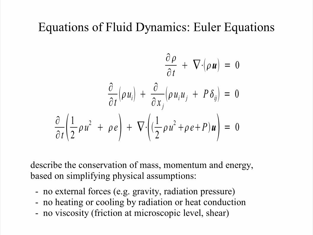
Equations of Fluid Dynamics: Euler Equations
describe the conservation of mass, momentum and energy,based on simplifying physical assumptions:
- no external forces (e.g. gravity, radiation pressure) - no heating or cooling by radiation or heat conduction - no viscosity (friction at microscopic level, shear)
∂∂ t 1
2 u2 e ∇⋅ 1
2 u2 eP u = 0
∂∂ t ui ∂
∂ x jui u j P ij = 0
∂∂ t
∇⋅u = 0
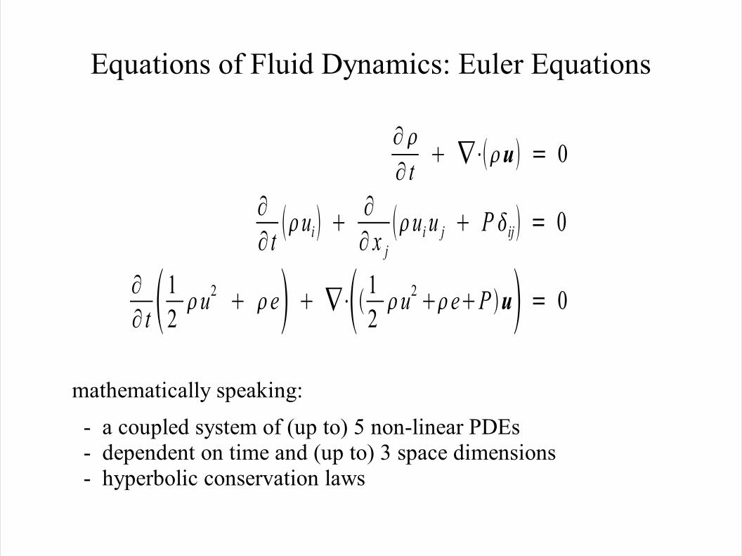
Equations of Fluid Dynamics: Euler Equations
mathematically speaking:
- a coupled system of (up to) 5 non-linear PDEs - dependent on time and (up to) 3 space dimensions - hyperbolic conservation laws
∂∂ t 1
2 u2 e ∇⋅ 1
2 u2 eP u = 0
∂∂ t ui ∂
∂ x jui u j P ij = 0
∂∂ t
∇⋅u = 0

Equations of Fluid Dynamics: Euler Equations
... in one space dimension, to simplify the following discussion
- a coupled system of 3 non-linear PDEs - dependent on time and 1 space dimension - hyperbolic conservation laws
∂∂ t 1
2 u2 e ∂
∂ x 1 2 u2 eP u = 0
∂∂ t u ∂
∂ x uu P = 0
∂∂ t
∂∂ x u = 0
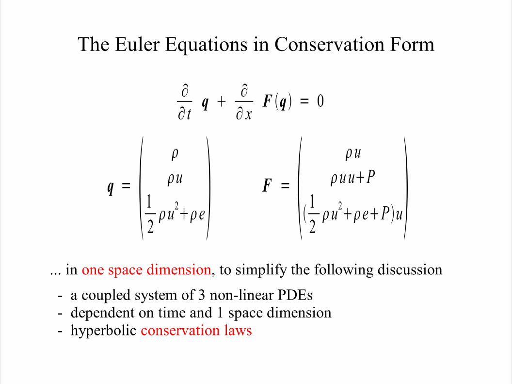
The Euler Equations in Conservation Form
∂∂ t
q ∂∂ x
F q = 0
q = u
1 2u2e F = u
u uP
1 2 u2eP u
... in one space dimension, to simplify the following discussion
- a coupled system of 3 non-linear PDEs - dependent on time and 1 space dimension - hyperbolic conservation laws

Mathematical Properties of PDEs
∂∂ t
q ∂∂ x
F q = 0
is a hyperbolic system if the Jacobian matrix of the flux function
has the following property: For each value of q the eigenvalues of F'(q) are real, and the matix is diagonalizable, i.e., there is a complete set of linearly independent eigenvectors.
F ' q = ∂F∂q
Properties of the Euler Equations
Some fundamental properties of the Euler equations may create difficulties for numerical solvers and make the analysis of discretization schemes more complicated:
- depending on the number of spatial dimensions, we have 3-5 coupled PDEs which need to be solved simultaneously
- non-linearity: even with smooth initial conditions the solutions have a tendency to develop discontinuities (shocks)
Goal:
Find simple limit cases (fewer equations, linear, if possible) which allows us to test certain aspects of numerical schemes before attacking the Euler equations in their full glory.

Euler Equations, Special Case: Passive Advection The Euler equations, 1D:
Assuming constant pressure P and a constant flow velocity u, the system of the Euler equations reduces to 2 separate linear PDEs:
∂∂ t 1
2 u2 e ∂
∂ x 1 2 u2 eP u = 0
∂∂ t u ∂
∂ x uu P = 0
∂∂ t
∂∂ x u = 0
∂∂ t
u∂∂ x
= 0∂e∂ t
u∂e∂ x
= 0
Euler Equations, Special Case: Passive Advection
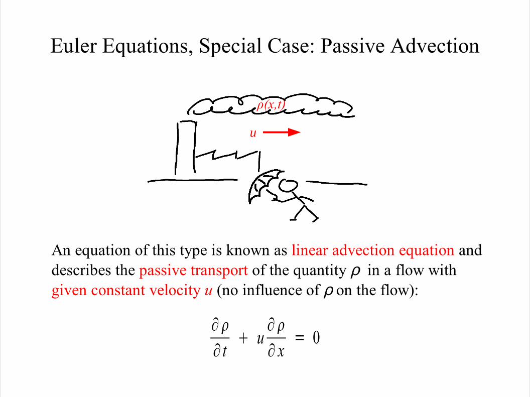
An equation of this type is known as linear advection equation and describes the passive transport of the quantity ρ in a flow with given constant velocity u (no influence of ρ on the flow):
∂∂ t
u∂∂ x
= 0
ρ(x,t)
u
Euler Equations, Special Case: Passive Advection
∂∂ t
u∂∂ x
= 0ρ(x,t)
u
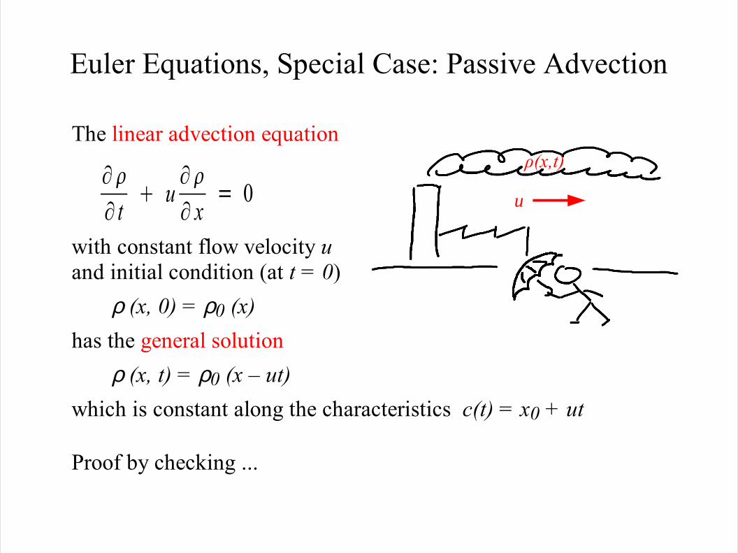
The linear advection equation
with constant flow velocity uand initial condition (at t = 0)
ρ (x, 0) = ρ0 (x)
has the general solution
ρ (x, t) = ρ0 (x – ut)
which is constant along the characteristics c(t) = x0 + ut
Proof by checking ...

Modification: Advection-Diffusion Equation
ρ(x,t)
u
∂∂ t
∂∂ x
u−D∂∂ x
= 0
A relative of the linear advectionequation (useful for numerics*):
The advection-diffusion equation
advective flux diffusive flux(transport due (diffusion due toto fluid motion) gradient in ρ) for constant u and D: with diffusion coefficient D > 0 * parabolic PDE, smooth solution!
advection
diffusion
∂∂ t u
∂∂ x = D
∂2 ∂ x2

Introduction to Numerical Hydrodynamics
2. The Linear Advection Equation
2.2 Naïve Numerics: Discretization Attempts

The Diffusion Equation
The diffusion equation (describing, e.g., heat conduction)
is a parabolic PDE. It always has a smooth solution for t > 0 even if the initial conditions are discontinuous.
Discretization in time and space: tn = n∆t + t0 xi = i∆x + x0
explicit Euler scheme
∂ y∂ t = D ∂2 y
∂ x2
∂ y∂ t
y i
n1− y in
t∂2 y∂ x2
y i1n − 2y i
n y i−1n
x2
⇒ yin1= y i
n t x2 D y i1
n − 2y in y i−1
n

The diffusion equation (describing, e.g., heat conduction)
is a parabolic PDE. It always has a smooth solution for t > 0 even if the initial conditions are discontinuous.
Discretization in time and space: tn = n∆t + t0 xi = i∆x + x0
explicit Euler scheme
The Diffusion Equation
∂ y∂ t = D ∂2 y
∂ x2
Stability of Euler scheme for the diffusion equation: Initial condition (red) and solution (blue) for D∆t/∆x2 = 0.2 (left), 0.4 (middle) and 0.6 (right)
stability: ∆t/∆x2 = (1/2D) positivity: ∆t/∆x2 = (1/4D)
Figu
res c
ourte
sy o
f Ber
nd F
reyt
ag
⇒ yin1= y i
n t x2 D y i1
n − 2y in y i−1
n

The Diffusion Equation
∂ y∂ t = D ∂2 y
∂ x2
Initial condition (red) and solution (blue) for D∆t/∆x2 = 0.1 (left) and 0.5 (right) after 500 and 100 time steps, respectively.
The slightly too large time step causes non-decaying spurious oscillations in the right panel.
The simple discretization gives reasonable results.
Figu
res c
ourte
sy o
f Ber
nd F
reyt
ag
The Linear Advection Equation
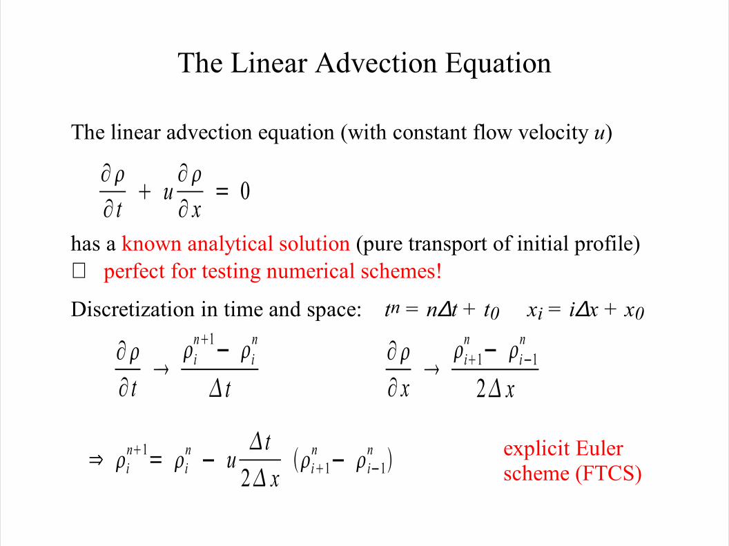
The linear advection equation (with constant flow velocity u)
has a known analytical solution (pure transport of initial profile)⇒ perfect for testing numerical schemes!
Discretization in time and space: tn = n∆t + t0 xi = i∆x + x0
explicit Euler scheme (FTCS)
∂∂ t
i
n1− in
t∂∂ x
i1
n − i−1n
2 x
⇒ in1= i
n − ut
2 xi1
n − i−1n
∂∂ t
u∂∂ x
= 0
The Linear Advection Equation
∂ y∂ t = D ∂2 y
∂ x2
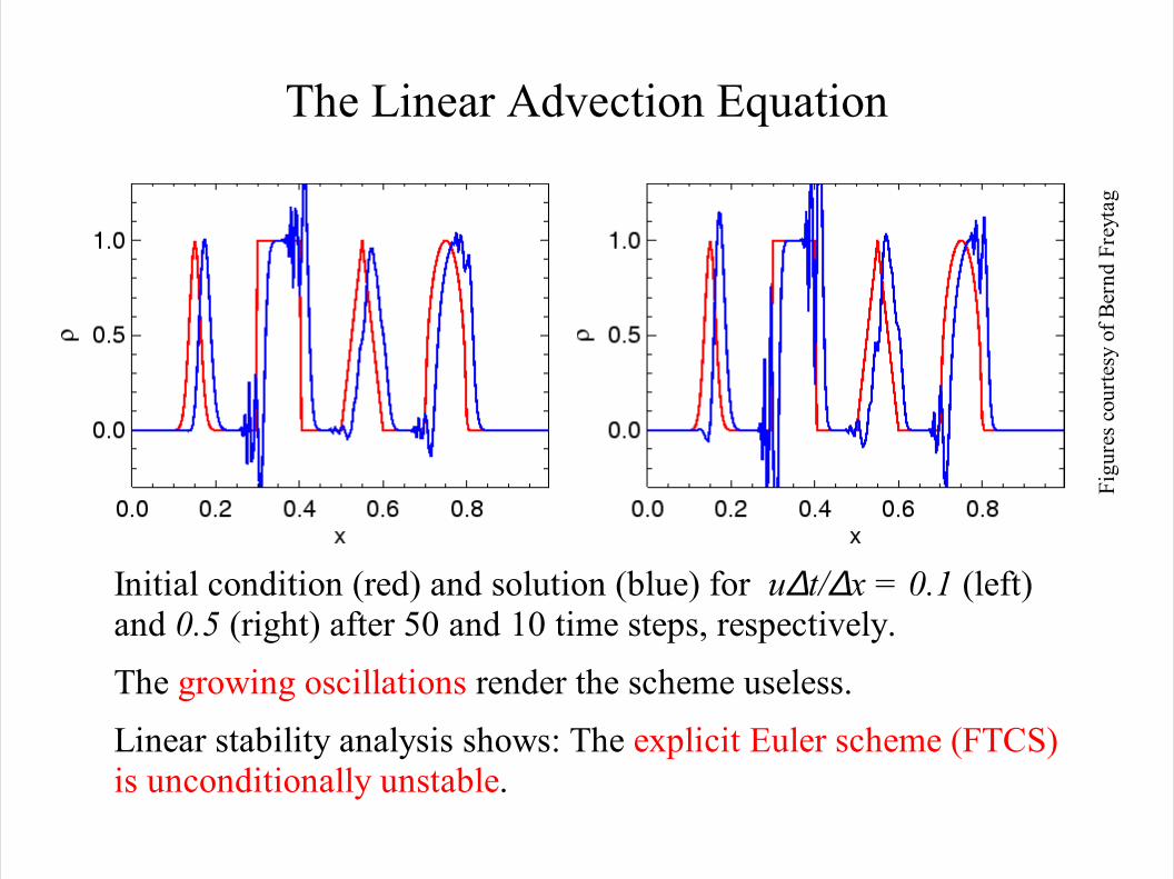
Initial condition (red) and solution (blue) for u∆t/∆x = 0.1 (left) and 0.5 (right) after 50 and 10 time steps, respectively.
The growing oscillations render the scheme useless. Linear stability analysis shows: The explicit Euler scheme (FTCS) is unconditionally unstable.
Figu
res c
ourte
sy o
f Ber
nd F
reyt
ag
Introduction to Numerical Hydrodynamics
2. The Linear Advection Equation
2.3 Basic Concepts and Tools
Discretization in Space: Concepts
Representation of the “real” distribution of a variable by a finite set of numbers (on a spatial grid)
Restriction: transformation from continuous values to discrete representation
Reconstruction: transformation from discrete representation to continuous values
Finite difference methods:
- restriction: sampling, e.g.: ρi = ρ(xi) - reconstruction: interpolation (polynomials) - derivatives become finite differences
Discretization in Space: Concepts
Representation of the “real” distribution of a variable by a finite set of numbers (on a spatial grid)
Restriction: transformation from continuous values to discrete representation
Reconstruction: transformation from discrete representation to continuous values
Finite volume methods:
- restriction: integration over control volume, e.g.:
- reconstruction: by polynomials - derivatives can become finite differences, or can be avoided
Discretization in Space: Concepts
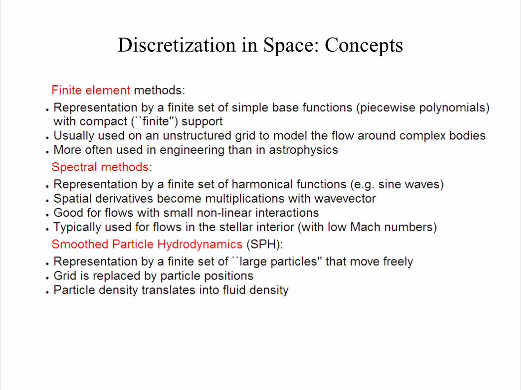
Finite element methods:
Discretization in Space: Concepts
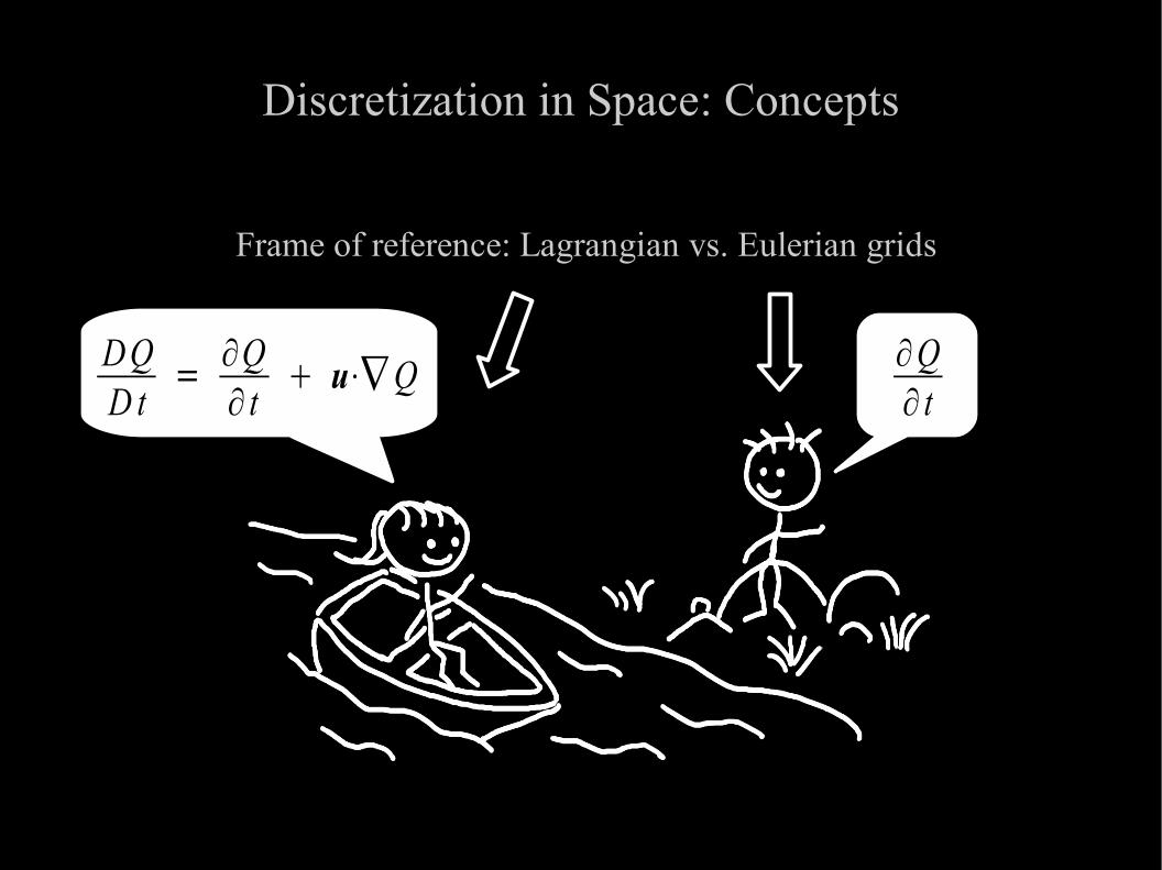
Frame of reference: Lagrangian vs. Eulerian grids
DQD t
= ∂Q∂ t
u⋅∇Q ∂Q∂ t
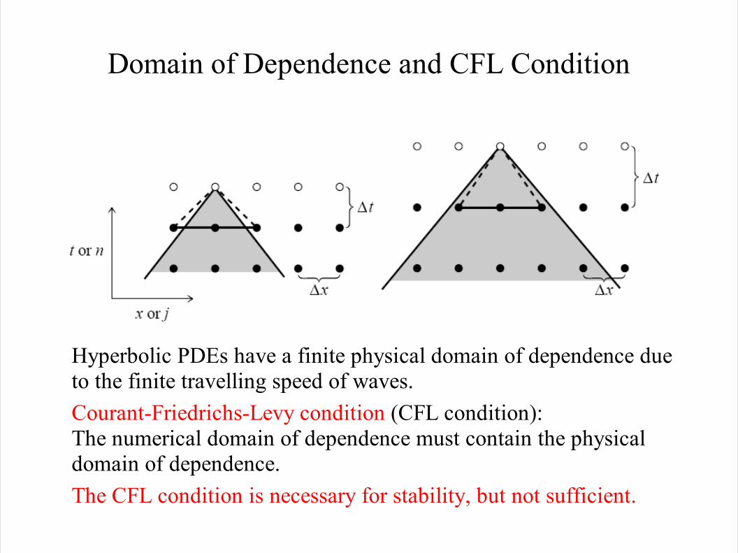
Domain of Dependence and CFL Condition
Hyperbolic PDEs have a finite physical domain of dependence due to the finite travelling speed of waves.
Courant-Friedrichs-Levy condition (CFL condition): The numerical domain of dependence must contain the physical domain of dependence.
The CFL condition is necessary for stability, but not sufficient.
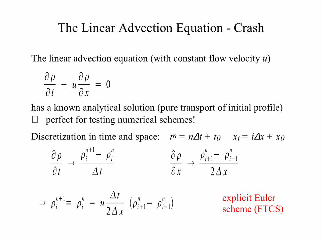
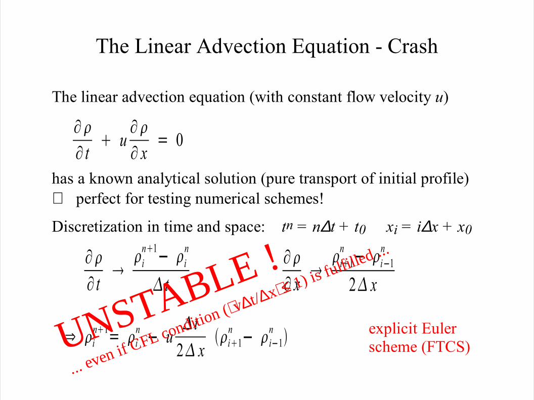
The Linear Advection Equation - Crash
The linear advection equation (with constant flow velocity u)
has a known analytical solution (pure transport of initial profile)⇒ perfect for testing numerical schemes!
Discretization in time and space: tn = n∆t + t0 xi = i∆x + x0
explicit Euler scheme (FTCS)
∂∂ t
i
n1− in
t∂∂ x
i1
n − i−1n
2 x
⇒ in1= i
n − ut
2 xi1
n − i−1n
∂∂ t
u∂∂ x
= 0
UNSTABLE !
... even if CFL condition (v∆t/∆x≤ 1) is f
ulfilled ...
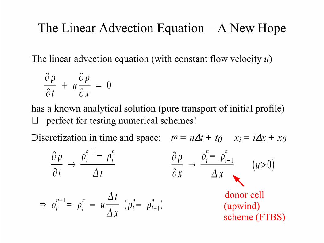
The Linear Advection Equation – A New Hope
The linear advection equation (with constant flow velocity u)
has a known analytical solution (pure transport of initial profile)⇒ perfect for testing numerical schemes!
Discretization in time and space: tn = n∆t + t0 xi = i∆x + x0
donor cell (upwind) scheme (FTBS)
∂∂ t
i
n1− in
t∂∂ x
i
n− i−1n
xu0
⇒ in1= i
n − u t x
in− i−1
n
∂∂ t
u∂∂ x
= 0
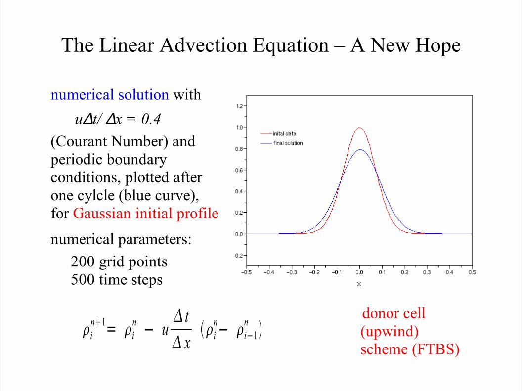
numerical solution with
u∆t/ ∆x = 0.4
(Courant Number) andperiodic boundary conditions, plotted after one cylcle (blue curve),for Gaussian initial profile
numerical parameters:
200 grid points 500 time steps

The Linear Advection Equation – A New Hope
The linear advection equation (with constant flow velocity u)
has a known analytical solution (pure transport of initial profile)⇒ perfect for testing numerical schemes!
Discretization in time and space: tn = n∆t + t0 xi = i∆x + x0
donor cell (upwind) scheme (FTBS)
∂∂ t
i
n1− in
t∂∂ x
i
n− i−1n
xu0
⇒ in1= i
n − u t x
in− i−1
n
∂∂ t
u∂∂ x
= 0
numerical solution with
u∆t/ ∆x = 0.4
(Courant Number) andperiodic boundary conditions, plotted after one cylcle (blue curve),for box initial profile
numerical parameters:
200 grid points 500 time steps

The Linear Advection Equation – Homework 1
Compute the numerical solution of the linear advection equation
using the upwind (donor cell) scheme*, with the initial conditions
for and for
in the range 0 ≤ x ≤ 1, assuming u=1 and ∆t/∆x = 0.5
Plot the resulting numerical solution and the exact analytical solution at time t = 0.5 for the cases ∆x = 0.01 and ∆x = 0.0025.
*upwind (donor cell) scheme ⇒ in1= i
n − u t x
in− i−1
n
∂∂ t
u∂∂ x
= 0
0 x = 1 x0 0 x = 0 x0


