Introduction toOptimization

Second Order Optimization Methods

Marc ToussaintU Stuttgart

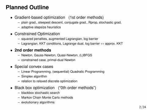
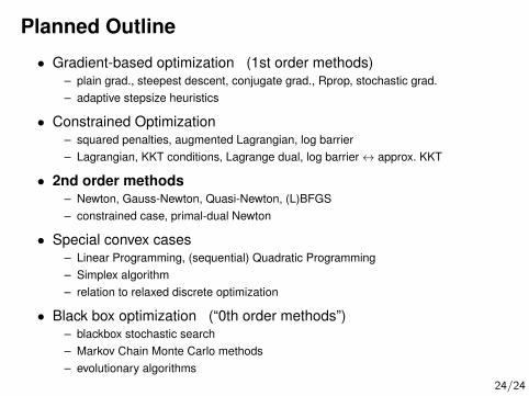
Planned Outline

• Gradient-based optimization (1st order methods)– plain grad., steepest descent, conjugate grad., Rprop, stochastic grad.– adaptive stepsize heuristics

• Constrained Optimization– squared penalties, augmented Lagrangian, log barrier– Lagrangian, KKT conditions, Lagrange dual, log barrier↔ approx. KKT

• 2nd order methods– Newton, Gauss-Newton, Quasi-Newton, (L)BFGS– constrained case, primal-dual Newton

• Special convex cases– Linear Programming, (sequential) Quadratic Programming– Simplex algorithm– relation to relaxed discrete optimization

• Black box optimization (“0th order methods”)– blackbox stochastic search– Markov Chain Monte Carlo methods– evolutionary algorithms

2/24

• So far we relied on gradient-based methods only, in the unconstrainedand constrained case

• Today: 2nd order methods, which approximate f(x) locally– using 2nd order Taylor expansion (Hessian ∇2f(x) given)– estimating the Hessian from data

• 2nd order methods only work if the Hessian is everywherepositive definite ↔ f(x) is convex

• Note: Approximating f(x) locally or globally is a core concept also inblack box optimization

3/24

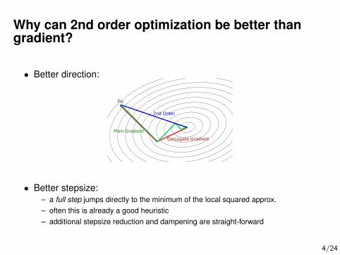
Why can 2nd order optimization be better thangradient?

• Better direction:

Conjugate Gradient

Plain Gradient

2nd Order

• Better stepsize:– a full step jumps directly to the minimum of the local squared approx.– often this is already a good heuristic– additional stepsize reduction and dampening are straight-forward

4/24

Outline: 2nd order method

• Newton

• Gauss-Newton

• Quasi-Newton

• BFGS, (L)BFGS

• Their application on constrained problems

5/24

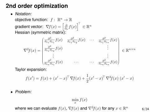
2nd order optimization• Notation:

objective function: f : Rn → R

gradient vector: ∇f(x) =[

∂∂xf(x)

]>∈ Rn

Hessian (symmetric matrix):

∇2f(x) =

∂2

∂x1∂x1

f(x) ∂2

∂x1∂x2

f(x) · · · ∂2

∂x1∂xn

f(x)

∂2

∂x1∂x2f(x)

......

...∂2

∂xn∂x1f(x) · · · · · · ∂2

∂xn∂xnf(x)

∈ Rn×n

Taylor expansion:

f(x′) = f(x) + (x′ − x)>∇f(x) +1

2(x′ − x)>∇2f(x) (x′ − x)

• Problem:

minxf(x)

where we can evaluate f(x), ∇f(x) and ∇2f(x) for any x ∈ Rn6/24

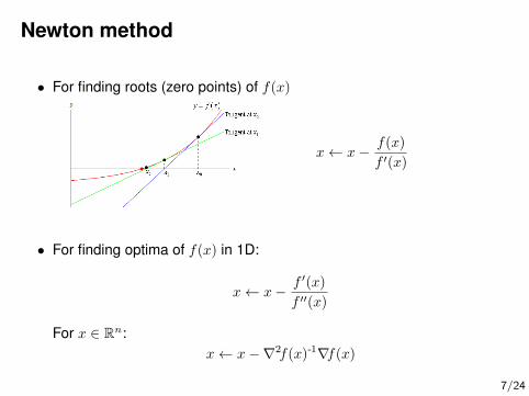
Newton method

• For finding roots (zero points) of f(x)

x← x− f(x)

f ′(x)

• For finding optima of f(x) in 1D:

x← x− f ′(x)

f ′′(x)

For x ∈ Rn:x← x−∇2f(x)-1∇f(x)

7/24

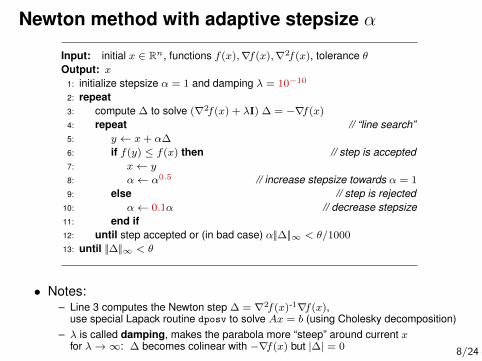
Newton method with adaptive stepsize α

Input: initial x ∈ Rn, functions f(x),∇f(x),∇2f(x), tolerance θOutput: x

1: initialize stepsize α = 1 and damping λ = 10−10

2: repeat3: compute ∆ to solve (∇2f(x) + λI) ∆ = −∇f(x)

4: repeat // “line search”5: y ← x+ α∆

6: if f(y) ≤ f(x) then // step is accepted7: x← y

8: α← α0.5 // increase stepsize towards α = 1

9: else // step is rejected10: α← 0.1α // decrease stepsize11: end if12: until step accepted or (in bad case) α||∆||∞ < θ/1000

13: until ||∆||∞ < θ

• Notes:– Line 3 computes the Newton step ∆ = ∇2f(x)-1∇f(x),

use special Lapack routine dposv to solve Ax = b (using Cholesky decomposition)– λ is called damping, makes the parabola more “steep” around current x

for λ→∞: ∆ becomes colinear with −∇f(x) but |∆| = 0 8/24

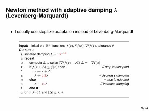
Newton method with adaptive damping λ(Levenberg-Marquardt)

• I usually use stepsize adaptation instead of Levenberg-Marquardt

Input: initial x ∈ Rn, functions f(x),∇f(x),∇2f(x), tolerance θOutput: x

1: initialize damping λ = 10−10

2: repeat3: compute ∆ to solve (∇2f(x) + λI) ∆ = −∇f(x)

4: if f(x+ ∆) ≤ f(x) then // step is accepted5: x← x+ ∆

6: λ← 0.2λ // decrease damping7: else // step is rejected8: λ← 10λ // increase damping9: end if

10: until λ < 1 and ||∆||∞ < δ

9/24

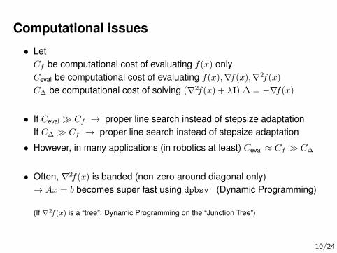
Computational issues

• LetCf be computational cost of evaluating f(x) onlyCeval be computational cost of evaluating f(x),∇f(x),∇2f(x)

C∆ be computational cost of solving (∇2f(x) + λI) ∆ = −∇f(x)

• If Ceval � Cf → proper line search instead of stepsize adaptationIf C∆ � Cf → proper line search instead of stepsize adaptation

• However, in many applications (in robotics at least) Ceval ≈ Cf � C∆

• Often, ∇2f(x) is banded (non-zero around diagonal only)→ Ax = b becomes super fast using dpbsv (Dynamic Programming)

(If ∇2f(x) is a “tree”: Dynamic Programming on the “Junction Tree”)

10/24

Demo

11/24

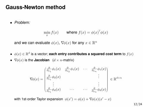
Gauss-Newton method

• Problem:

minxf(x) where f(x) = φ(x)>φ(x)

and we can evaluate φ(x), ∇φ(x) for any x ∈ Rn

• φ(x) ∈ Rd is a vector; each entry contributes a squared cost term to f(x)

• ∇φ(x) is the Jacobian (d× n-matrix)

∇φ(x) =

∂∂x1

φ1(x)∂∂x2

φ1(x) · · · ∂∂xn

φ1(x)

∂∂x1

φ2(x)...

......

∂∂x1

φd(x) · · · · · · ∂∂xn

φd(x)

∈ Rd×n

with 1st-order Taylor expansion φ(x′) = φ(x) +∇φ(x)(x′ − x)12/24

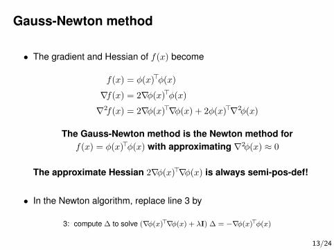
Gauss-Newton method

• The gradient and Hessian of f(x) become

f(x) = φ(x)>φ(x)

∇f(x) = 2∇φ(x)>φ(x)

∇2f(x) = 2∇φ(x)>∇φ(x) + 2φ(x)>∇2φ(x)

The Gauss-Newton method is the Newton method forf(x) = φ(x)>φ(x) with approximating ∇2φ(x) ≈ 0

The approximate Hessian 2∇φ(x)>∇φ(x) is always semi-pos-def!

• In the Newton algorithm, replace line 3 by

3: compute ∆ to solve (∇φ(x)>∇φ(x) + λI) ∆ = −∇φ(x)>φ(x)

13/24

Quasi-Newton methods

14/24

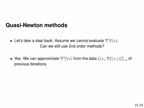
Quasi-Newton methods

• Let’s take a step back: Assume we cannot evaluate ∇2f(x).Can we still use 2nd order methods?

• Yes: We can approximate ∇2f(x) from the data {(xi,∇f(xi))}ki=1 ofprevious iterations

15/24

Basic example

• We’ve seen already two data points (x1,∇f(x1)) and (x2,∇f(x2))

How can we estimate ∇2f(x)?

• In 1D:

∇2f(x) ≈ ∇f(x2)−∇f(x1)

x2 − x1

• In Rn: let y = ∇f(x2)−∇f(x1), ∆x = x2 − x1

∇2f(x) ∆x!= y ∆x

!= ∇2f(x)−1y

∇2f(x) =y y>

y>∆x∇2f(x)−1 =

∆x∆x>

∆x>y

Convince yourself that the last line solves the desired relations[Left: how to update ∇2f (x). Right: how to update directly ∇2f(x)-1.]

16/24

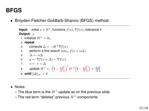
BFGS

• Broyden-Fletcher-Goldfarb-Shanno (BFGS) method:

Input: initial x ∈ Rn, functions f(x),∇f(x), tolerance θOutput: x

1: initialize H-1 = In2: repeat3: compute ∆ = −H-1∇f(x)

4: perform a line search minα f(x+ α∆)

5: ∆← α∆

6: y ← ∇f(x+ ∆)−∇f(x)

7: x← x+ ∆

8: update H-1 ←(I− y∆>

∆>y

)>H-1

(I− y∆>

∆>y

)+ ∆∆>

∆>y9: until ||∆||∞ < θ

• Notes:– The blue term is the H-1-update as on the previous slide– The red term “deletes” previous H-1-components

17/24

Quasi-Newton methods

• BFGS is the most popular of all Quasi-Newton methodsOthers exist, which differ in the exact H -1-update

• L-BFGS (limited memory BFGS) is a version which does not require toexplicitly store H -1 but instead stores the previous data{(xi,∇f(xi))}ki=1 and manages to compute ∆ = −H -1∇f(x) directlyfrom this data

• Some thought:In principle, there are alternative ways to estimate H -1 from the data{(xi, f(xi),∇f(xi))}ki=1, e.g. using Gaussian Process regression withderivative observations

– Not only the derivatives but also the value f(xi) should give information on H(x) fornon-quadratic functions

– Should one weight ‘local’ data stronger than ‘far away’?(GP covariance function)

18/24

2nd Order Methods for Constrained Optimization

19/24

2nd Order Methods for Constrained Optimization

• No changes at all for– log barrier– augmented Lagrangian– squared penalties

Directly use (Gauss-)Newton/BFGS→ will boost performance of theseconstrained optimization methods!

20/24

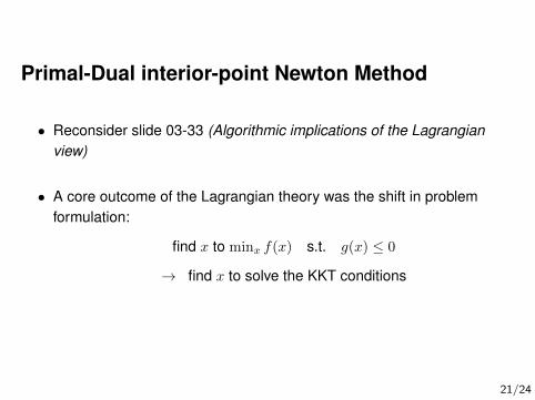
Primal-Dual interior-point Newton Method

• Reconsider slide 03-33 (Algorithmic implications of the Lagrangianview)

• A core outcome of the Lagrangian theory was the shift in problemformulation:

find x to minx f(x) s.t. g(x) ≤ 0

→ find x to solve the KKT conditions

21/24

Primal-Dual interior-point Newton Method• The first and last modified (=approximate) KKT conditions

∇f(x) +∑m

i=1 λi∇gi(x) = 0 (“force balance”)

∀i : gi(x) ≤ 0 (primal feasibility)

∀i : λi ≥ 0 (dual feasibility)

∀i : λigi(x) = −µ (complementary)

can be written as the n+m-dimensional equation system

r(x, λ) = 0 , r(x, λ) :=

∇f(x) + λ>∇g(x)

−diag(λ)g(x)− µ1n

• Newton method to find the root r(x, λ) = 0xλ

←xλ

−∇r(x, λ)-1r(x, λ)

∇r(x, λ) =

∇2f(x) +

∑i λi∇2gi(x) ∇g(x)>

−diag(λ)∇g(x) −diag(g(x))

∈ R(n+m)×(n+m)

22/24

Primal-Dual interior-point Newton Method

• The method requires the Hessians ∇2f(x) and ∇2gi(x)

– One can approximate the constraint Hessians ∇2gi(x) ≈ 0

– Gauss-Newton case: f(x) = φ(x)>φ(x) only requires ∇φ(x)

• This primal-dual method does a joint update of both– the solution x– the lagrange multipliers (constraint forces) λNo need for nested iterations, as with penalty/barrier methods!

• The above formulation allows for a duality gap µ; choose µ = 0 orconsult Boyd how to update on the fly (sec 11.7.3)

• The feasibility constraints gi(x) ≤ 0 and λi ≥ 0 need to be handledexplicitly by the root finder (the line search needs to ensure theseconstraints)

23/24

Planned Outline

• Gradient-based optimization (1st order methods)– plain grad., steepest descent, conjugate grad., Rprop, stochastic grad.– adaptive stepsize heuristics

• Constrained Optimization– squared penalties, augmented Lagrangian, log barrier– Lagrangian, KKT conditions, Lagrange dual, log barrier↔ approx. KKT

• 2nd order methods– Newton, Gauss-Newton, Quasi-Newton, (L)BFGS– constrained case, primal-dual Newton

• Special convex cases– Linear Programming, (sequential) Quadratic Programming– Simplex algorithm– relation to relaxed discrete optimization

• Black box optimization (“0th order methods”)– blackbox stochastic search– Markov Chain Monte Carlo methods– evolutionary algorithms

24/24