Introduction to Patterns, Pro les and Hidden Markov...

Introduction to Patterns, Profiles and HiddenMarkov Models

Marco PagniSwiss Institute of Bioinformatics (SIB)

30th August 2002

EMBNET Course 2002 Introduction to Patterns, Profiles and HMMs

Multiple alignments

1


Multiple sequence alignment (MSA)

. The alignment of multiple sequences is a method of choice to detect conservedregions in protein or DNA sequences. These particular regions are usuallyassociated with:

. Signals (promoters, signatures for phosphorylation, cellular location, ...);

. Structure (correct folding, protein-protein interactions...);

. Chemical reactivity (catalytic sites,... ).

. The information represented by these regions can be used to align sequences,search similar sequences in the databases or annotate new sequences.

. Different methods exist to build models of these conserved regions:

. Consensus sequences;

. Patterns;

. Position Specific Score Matrices (PSSMs);

. Profiles;

. Hidden Markov Models (HMMs),

. ... and a few others.

2


Multiple alignments reflect secondary structures

STA3_MOUSEZA70_MOUSEZA70_HUMANPIG2_RATMATK_HUMANSEM5_CAEELP85B_BOVINVAV_MOUSEYES_XIPHETXK_HUMANPIG2_HUMANYKF1_CAEELSPK1_DUGTISTA6_HUMANSTA4_MOUSESPT6_YEAST

.AEGQNEAKNTEWQK.

EEEEEDEGDQSDEYEQ

RAAAAAVATAAVAVKA

EEEEVENEEEEFETEE

RERDQVEGRHKQKSRD

AHKMQLKILLLLSLLY

ILLLLLLLLLLLLLLL

LKYMQKRTLRQDMLLR

SLSRPKDNLQENKNKS

|10

.AG..P..P.Y.I...

.

.

.

.

.

.

.

.

.

.C.....

.

.

.

.

.

.

.

.

.

.M.....

.

.

.

.

.

.

.

.

.

.E.....

.

.

.

.

.

.

.

.

.

.T.....

TGAI.T..GEG.G.D.

KMQPPVTRNSG.LEKK

PATRERPSEKK.QPME

PDDDDDDDREDNKDPR

GGGGGGGGGGGGGGGG

|20

TLKALHTTTATDTTTE

FFFFFFFYFFFYYFFF

LLLLLLLLLILVILLV

LLLIVVVVIVVVILLI

RRRRRRRRRRRRRRRR

FQPKEQDQEDELPFFQ

SCRRSCARSSSSSSSS

ELKEAESVEREDRDES

SREGRSSKT.TP.SSR

S.....K.........

|30

KS.THSIDTHFKKEHG

ELQDPPQTKLPPEILD

GGG.GGGAGGNGNGGD

GGTSDEEEASDESGGH

.

.

.

.

.

.

.

.

.

.

.P....

.

.

.

.

.

.

.

.

.

.

.R....

.

.

.

.

.

.

.

.

.

.

.S....

VYYYYFYFYYYYYIIL

TVAAVSTASTTIATTV

FLLILILILILLLIFI

|40

TSSTCSTSSSSSSATT

WLLFVVLILVFVVHWW

VVIRSRRKRFWMRVVK

EHYAFFKYDMRFDIDL

KDGRGQGNWGSNFRQD

DVKGRDGVDAGNDGSK

I.......ER.KEQ.D

S.......TR.LKD..

G.......KS.DKG..

K........T.EK...

|50

T...............

.

.

.

.

.

.

.

.

.

.

.

.

.

.

.

.

Q...............

I.......GE.NIS..

Q.......DA.SCP..

SRTKDSNENARSIQEL

VFVVVVNVCIVVVINF

EHYKIQKKKKQKKEGQ

PHHHHHLHHHHHHNEH

YFYCYF.IYYCFFIVI

|60

TPLRRKIKKQRVQQRD

KIIIVVKIIIIIIPFI

QESNLLVMRKRNKFHQ

QRQRHRFTKKSSTSSE

LQDDRDHSLNTVLAVL

NLKGDQREDDMEQKEE

STA3_MOUSEZA70_MOUSEZA70_HUMANPIG2_RATMATK_HUMANSEM5_CAEELP85B_BOVINVAV_MOUSEYES_XIPHETXK_HUMANPIG2_HUMANYKF1_CAEELSPK1_DUGTISTA6_HUMANSTA4_MOUSESPT6_YEAST

NNARGNDGNSENDDPK

MGG..GG.GGGKEL.E

S.........G.K..N

F.........T....P

|70

A..............L

E...............

I..............A

I..............L

M.........L....G

GTKHH...GQK.G..K

YYYFLKHLYWYYIS.V

KACVTYYYYYYFSIYL

IIILIYGRIVLVYRNI

MAPGDLFITATNSSKV

|80

DGETEWSTTEDNVLGD

.GGSAAEERRNNNGRN

AKTAVVPKTHLMIDLQ

TAKYFKLKQARSRRSK

.

.

.

.

.

.TA....N...

.

.

.

.

.

.

.

.

.

.

.

.

.

.

.

.

NHFFFFFFFFFFFIAY

ICDECNCRMQRNPRLN

LGTSNSSGSSRTNDAD

VPLLLLVLLIMIILFL

|90

SAWVMNVLQPYQLAAD

PEQEDEDEMEAQTQDQ

LLLLMLLLLLLMLLII

VCVVVVIVVIILIKLI

YQESEATEKWQSQNRV

LFYYHYHFHYHHFLDE

YYLYYHYYYHYYYYYY

3


Multiple alignments reflect secondary structures

4


Consensus sequences

5


Consensus sequences

. The consensus sequence method is the simplest method to build a model from amultiple sequence alignment.

. The consensus sequence is built using the following rules:

. Majority wins.

. Skip too much variation.

6


How to build consensus sequences

Search databases

K K Y F E D R A P S S

L E P K G C P L E C R T T F M

Jalview Michele Clamp 1998

sp|P54202|ADH2_EMENIsp|P16580|GLNA_CHICKsp|P40848|DHP1_SCHPOsp|P57795|ISCS_METTEsp|P15215|LMG1_DROME

GGGGG

HHHHH

EEEEE

GKGFL

VKYER

GGGGG

KYGPT

VFRKT

VESGF

|10

KDRCM

LRGGP

GGGAA

APGLL

GSYYE

AASIC

G H E G V G K V V K L G A G A

F Y G R S R G G Y I

1 2 3 4 5 6 7 8 9 10 11 12 13 14 15

Consensus: GHE--G-----G---

7


Consensus sequences

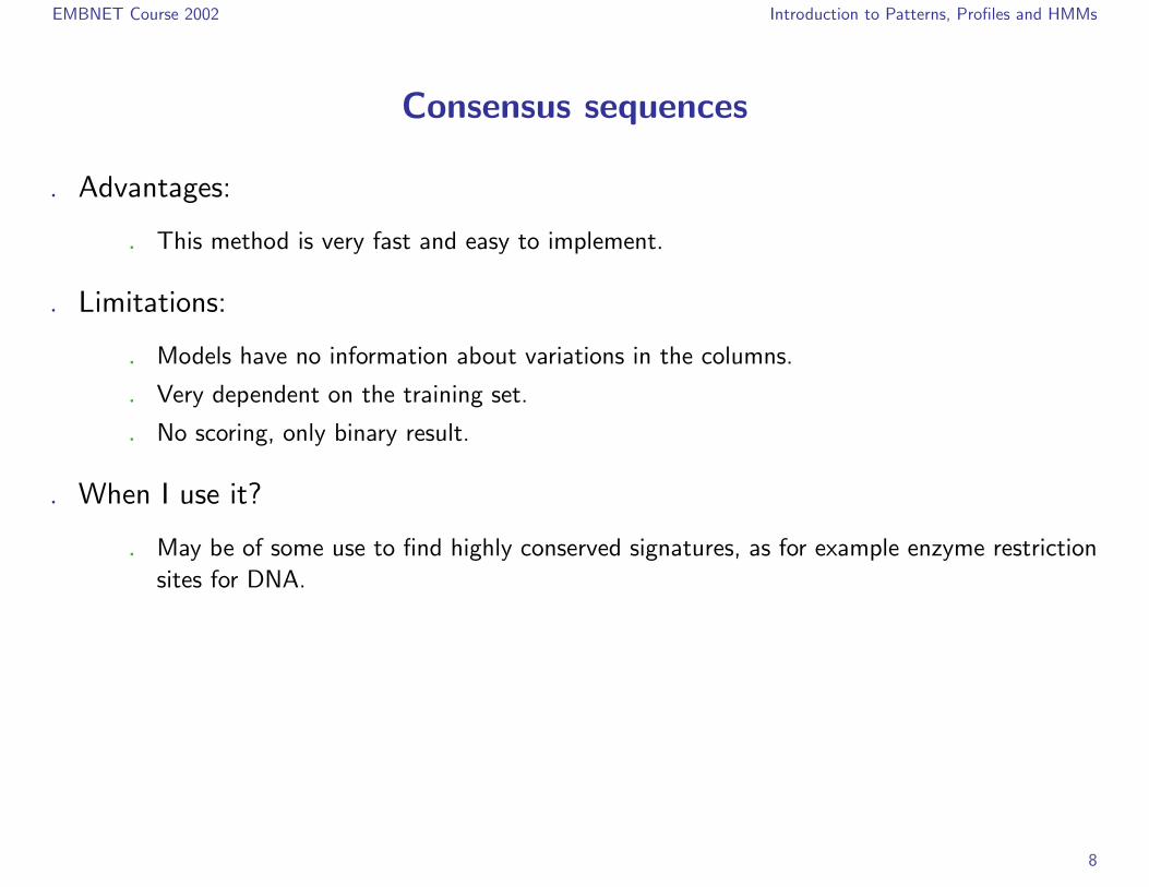
. Advantages:

. This method is very fast and easy to implement.

. Limitations:

. Models have no information about variations in the columns.

. Very dependent on the training set.

. No scoring, only binary result.

. When I use it?

. May be of some use to find highly conserved signatures, as for example enzyme restriction

sites for DNA.

8


Pattern matching

9


Pattern syntax

. A pattern describes a set of alternative sequences, using a single expression. Incomputer science, patterns are known as regular expressions.

. The Prosite syntax for patterns:

. uses the standard IUPAC one-letter codes for amino acids (G=Gly, P=Pro, ...),

. each element in a pattern is separated from its neighbor by a ’-’,

. the symbol ’X’ is used where any amino acid is accepted,

. ambiguities are indicated by square parentheses ’[ ]’ ([AG] means Ala or Gly),

. amino acids that are not accepted at a given position are listed between a pair of curly

brackets ’{ }’ ({AG} means any amino acid except Ala and Gly),

. repetitions are indicated between parentheses ’( )’ ([AG](2,4) means Ala or Gly between 2

and 4 times, X(2) means any amino acid twice),

. a pattern is anchored to the N-term and/or C-term by the symbols ’<’ and ’>’ respectively.

10


Pattern syntax: an example

. The following pattern

<A-x-[ST](2)-x(0,1)-{V}

. means:

. an Ala in the N-term,

. followed by any amino acid,

. followed by a Ser or Thr twice,

. followed or not by any residue,

. followed by any amino acid except Val.

11


How to build a pattern

Search databases

G H E G V G K V V K L G A G A K K Y F E D R A P S S F Y G R S R G G Y I

R T T F M L E P K G C P L E C



GGGGG

HHHHH

EEEEE

GKGFL

VKYER

GGGGG

KYGPT

VFRKT

VESGF

|10

KDRCM

LRGGP

GGGAA

APGLL

GSYYE

AASIC

Profile: G-H-E-X(2)-G-X(5)-[GA]-X(3)

1 2 3 4 5 6 7 8 9 10 11 12 13 14 15

12


Pattern examples

. Patterns and PSSMs are appropriate to build models of short sequence signatures.

. Example of short signatures:

. Post-translational signatures:

. Protein splicing signature: [DNEG]-x-[LIVFA]-[LIVMY]-[LVAST]-H-N-[STC]

. Tyrosine kinase phosphorylation site: [RK]-x(2)-[DE]-x(3)-Y or [RK]-x(3)-[DE]-

x(2)-Y

. ...

. DNA-RNA interaction signatures:

. Histone H4 signature: G-A-K-R-H

. p53 signature: M-C-N-S-S-C-[MV]-G-G-M-N-R-R

. ...

. Enzymes:

. L-lactate dehydrogenase active site: [LIVMA]-G-[EQ]-H-G-[DN]-[ST]

. Ubiquitin-activating enzyme signature: P-[LIVM]-C-T-[LIVM]-[KRH]-x-[FT]-P

. ...

13


Patterns: Conclusion

. Advantages:

. Pattern matching is fast and easy to implement.

. Models are easy to design for anyone with some training in biochemistry.

. Models are easy to understand for anyone with some training in biochemistry.

. Limitations:

. Poor model for insertions/deletions (indels).

. Small patterns find a lot of false positives. Long patterns are very difficult to design.

. Poor predictors that tend to recognize only the sequence of the training set.

. No scoring system, only binary response.

. When I use patterns?

. To search for small signatures or active sites.

. To communicate with other biologists.

14


Patterns: beyond the conclusion

. Patterns can be automatically extracted (discovered) from a set of unalignedsequences by specialized programs.

. Pratt, Splash and Teiresas are three of these specialized programs.

. Today machine learning is a very active research field

. Such automatic patterns are usually distinct from those designed by an expertwith some knownledge of the biochemical litterature.

15


Position Specific ScoringMatrice (PSSM)

16


How to build a PSSM

. A PSSM is based on the frequencies of each residue in a specific position of amultiple alignment.

0 0 0 0 0 0 0 0 0 0 0 0 0 0 1

5 0 0 2 0 5 1 0 1 0 2 3 1 1 0

0 0 5 0 1 0 0 0 1 0 0 0 0 1 0

0 0 0 0 0 0 0 0 0 0 0 0 0 0 0

0 0 0 1 0 0 0 0 0 0 1 0 2 0 0

0 0 0 0 0 0 0 0 0 0 0 2 1 0 2

0 0 0 0 1 0 0 1 0 1 1 0 0 0 0

0 0 0 0 0 0 0 0 0 0 0 0 0 0 0

0 0 0 0 0 0 0 0 0 0 1 0 1 0 0

0 0 0 0 0 0 0 0 0 0 0 0 0 0 0

0 0 0 0 0 0 0 0 0 1 0 0 0 0 0

0 0 0 0 1 0 0 1 1 0 0 0 0 0 0

0 0 0 0 0 0 1 1 0 0 0 0 0 0 0

0 0 0 0 0 0 0 0 0 0 0 0 0 0 0

0 0 0 0 1 0 1 0 0 0 0 0 0 1 0

0 0 0 1 1 0 1 1 0 1 0 0 0 0 0

0 5 0 0 0 0 0 0 0 0 0 0 0 0 0

0 0 0 1 0 0 0 0 1 0 0 0 0 0 0

0 0 0 0 0 0 0 0 1 0 0 0 0 1 0

0 0 0 0 0 0 0 0 0 1 0 0 0 0 1



GGGGG

HHHHH

EEEEE

GKGFL

VKYER

GGGGG

KYGPT

VFRKT

VESGF

|10

KDRCM

LRGGP

GGGAA

APGLL

GSYYE

AASIC

1 2 3 4 5 6 7 8 9 10 11 12 13 14 15

A

C

D

E

F

G

H

I

K

L

M

N

P

Q

R

S

T

V

W

Y

. . Column 1: fA,1 = 05 = 0, fG,1 = 5

5 = 1, ...

. Column 2: fA,2 = 05 = 0, fH,2 = 5

5 = 1, ...

. ...

. Column 15: fA,15 = 25 = 0.4, fC,15 = 1

5 = 0.2, ...

17


Pseudo-counts

. Some observed frequencies usually equal 0. This is a consequence of the limitednumber of sequences that is present in a MSA.

. Unfortunately, an observed frequency of 0 might imply the exclusion of thecorresponding residue at this position position (this was the case with patterns).

. One possible trick is to add a small number to all observed frequencies. Thesesmall non-observed frequencies are refered to as a pseudo-counts.

. From the previous example with a pseudo-counts of 1:

. Column 1: f ′A,1 = 0+15+20 = 0.04, f ′G,1 = 5+1

5+20 = 0.24, ...

. Column 2: f ′A,2 = 0+15+20 = 0.04, f ′H,2 = 5+1

5+20 = 0.24, ...

. ...

. Column 15: f ′A,15 = 2+15+20 = 0.12, f ′C,15 = 1+1

5+20 = 0.08, ...

. There exist more sophisticated methods to produce more “realistic” pseudo-counts,and which are based on substitution matrix or Dirichlet mixtures.

18


Computing a PSSM

. The frequency of every residue determined at every position has to be comparedwith the frequency at which any residue can be expected in a random sequence.

. For example, let’s postulate that each amino acid is observed with an identicalfrequency in a random sequence. This is a quite simplisitic null model.

. The score is derived from the ratio of the observed to the expected frequencies.More precisely, the logarithm of this ratio is taken and refered to as the log-likelihood ratio:

Scoreij = log(f′ij

qi)

where Scoreij is the score for residue i at position j, f ′ij is the relative frequency

for a residue i at position j (corrected with pseudo-counts) and qi is the expectedrelative frequency of residue i in a random sequence.

19


Example

. The complete position specific scoring matrix calculated from the previous example:

1 2 3 4 5 6 7 8 9 10 11 12 13 14 15

A -0.2 -0.2 -0.2 -0.2 -0.2 -0.2 -0.2 -0.2 -0.2 -0.2 -0.2 1.3 0.7 -0.2 1.3C -0.2 -0.2 -0.2 -0.2 -0.2 -0.2 -0.2 -0.2 -0.2 0.7 -0.2 -0.2 -0.2 -0.2 0.7D -0.2 -0.2 -0.2 -0.2 -0.2 -0.2 -0.2 -0.2 -0.2 -0.2 -0.2 -0.2 -0.2 -0.2 -0.2E -0.2 -0.2 2.3 -0.2 0.7 -0.2 -0.2 -0.2 0.7 -0.2 -0.2 -0.2 -0.2 0.7 -0.2F -0.2 -0.2 -0.2 0.7 -0.2 -0.2 -0.2 -0.2 0.7 -0.2 -0.2 -0.2 -0.2 -0.2 -0.2G 2.3 -0.2 -0.2 1.3 -0.2 2.3 0.7 -0.2 0.7 -0.2 1.3 1.7 0.7 0.7 -0.2H -0.2 2.3 -0.2 -0.2 -0.2 -0.2 -0.2 -0.2 -0.2 -0.2 -0.2 -0.2 -0.2 -0.2 -0.2I -0.2 -0.2 -0.2 -0.2 -0.2 -0.2 -0.2 -0.2 -0.2 -0.2 -0.2 -0.2 -0.2 -0.2 0.7K -0.2 -0.2 -0.2 0.7 0.7 -0.2 0.7 0.7 -0.2 0.7 -0.2 -0.2 -0.2 -0.2 -0.2L -0.2 -0.2 -0.2 0.7 -0.2 -0.2 -0.2 -0.2 -0.2 -0.2 0.7 -0.2 1.3 -0.2 -0.2M -0.2 -0.2 -0.2 -0.2 -0.2 -0.2 -0.2 -0.2 -0.2 0.7 -0.2 -0.2 -0.2 -0.2 -0.2N -0.2 -0.2 -0.2 -0.2 -0.2 -0.2 -0.2 -0.2 -0.2 -0.2 -0.2 -0.2 -0.2 -0.2 -0.2P -0.2 -0.2 -0.2 -0.2 -0.2 -0.2 -0.2 -0.2 -0.2 -0.2 0.7 -0.2 0.7 -0.2 -0.2Q -0.2 -0.2 -0.2 -0.2 -0.2 -0.2 -0.2 -0.2 -0.2 -0.2 -0.2 -0.2 -0.2 -0.2 -0.2R -0.2 -0.2 -0.2 -0.2 0.7 -0.2 -0.2 0.7 -0.2 0.7 0.7 -0.2 -0.2 -0.2 -0.2S -0.2 -0.2 -0.2 -0.2 -0.2 -0.2 -0.2 -0.2 0.7 -0.2 -0.2 -0.2 -0.2 0.7 -0.2T -0.2 -0.2 -0.2 -0.2 -0.2 -0.2 0.7 0.7 -0.2 -0.2 -0.2 -0.2 -0.2 -0.2 -0.2V -0.2 -0.2 -0.2 -0.2 0.7 -0.2 -0.2 0.7 0.7 -0.2 -0.2 -0.2 -0.2 -0.2 -0.2W -0.2 -0.2 -0.2 -0.2 -0.2 -0.2 -0.2 -0.2 -0.2 -0.2 -0.2 -0.2 -0.2 -0.2 -0.2Y -0.2 -0.2 -0.2 -0.2 0.7 -0.2 0.7 -0.2 -0.2 -0.2 -0.2 -0.2 -0.2 0.7 -0.2

20


How to use PSSMs

. The PSSM is applied as a sliding window along the subject sequence:

. At every position, a PSSM score is calculated by summing the scores of all columns;

. The highest scoring position is reported.

T -0.2 -0.2 -0.2 -0.2 -0.2 -0.2 0.7 0.7 -0.2 -0.2 -0.2 -0.2 -0.2 -0.2 -0.2V -0.2 -0.2 -0.2 -0.2 0.7 -0.2 -0.2 0.7 0.7 -0.2 -0.2 -0.2 -0.2 -0.2 -0.2

1 2 3 4 5 6 7 8 9 10 11 12 13 14 15

Y -0.2 -0.2 -0.2 -0.2 0.7 -0.2 0.7 -0.2 -0.2 -0.2 -0.2 -0.2 -0.2 0.7 -0.2W -0.2 -0.2 -0.2 -0.2 -0.2 -0.2 -0.2 -0.2 -0.2 -0.2 -0.2 -0.2 -0.2 -0.2 -0.2

D -0.2 -0.2 -0.2 -0.2 -0.2 -0.2 -0.2 -0.2 -0.2 -0.2 -0.2 -0.2 -0.2 -0.2 -0.2

Y -0.2 -0.2 -0.2 -0.2 0.7 -0.2 0.7 -0.2 -0.2 -0.2 -0.2 -0.2 -0.2 0.7 -0.2

S -0.2 -0.2 -0.2 -0.2 -0.2 -0.2 -0.2 -0.2 0.7 -0.2 -0.2 -0.2 -0.2 0.7 -0.2R -0.2 -0.2 -0.2 -0.2 0.7 -0.2 -0.2 0.7 -0.2 0.7 0.7 -0.2 -0.2 -0.2 -0.2Q -0.2 -0.2 -0.2 -0.2 -0.2 -0.2 -0.2 -0.2 -0.2 -0.2 -0.2 -0.2 -0.2 -0.2 -0.2P -0.2 -0.2 -0.2 -0.2 -0.2 -0.2 -0.2 -0.2 -0.2 -0.2 0.7 -0.2 0.7 -0.2 -0.2N -0.2 -0.2 -0.2 -0.2 -0.2 -0.2 -0.2 -0.2 -0.2 -0.2 -0.2 -0.2 -0.2 -0.2 -0.2M -0.2 -0.2 -0.2 -0.2 -0.2 -0.2 -0.2 -0.2 -0.2 0.7 -0.2 -0.2 -0.2 -0.2 -0.2L -0.2 -0.2 -0.2 0.7 -0.2 -0.2 -0.2 -0.2 -0.2 -0.2 0.7 -0.2 1.3 -0.2 -0.2K -0.2 -0.2 -0.2 0.7 0.7 -0.2 0.7 0.7 -0.2 0.7 -0.2 -0.2 -0.2 -0.2 -0.2I -0.2 -0.2 -0.2 -0.2 -0.2 -0.2 -0.2 -0.2 -0.2 -0.2 -0.2 -0.2 -0.2 -0.2 0.7H -0.2 2.3 -0.2 -0.2 -0.2 -0.2 -0.2 -0.2 -0.2 -0.2 -0.2 -0.2 -0.2 -0.2 -0.2G 2.3 -0.2 -0.2 1.3 -0.2 2.3 0.7 -0.2 0.7 -0.2 1.3 1.7 0.7 0.7 -0.2F -0.2 -0.2 -0.2 0.7 -0.2 -0.2 -0.2 -0.2 0.7 -0.2 -0.2 -0.2 -0.2 -0.2 -0.2E -0.2 -0.2 2.3 -0.2 0.7 -0.2 -0.2 -0.2 0.7 -0.2 -0.2 -0.2 -0.2 0.7 -0.2

W -0.2 -0.2 -0.2 -0.2 -0.2 -0.2 -0.2 -0.2 -0.2 -0.2 -0.2 -0.2 -0.2 -0.2 -0.2V -0.2 -0.2 -0.2 -0.2 0.7 -0.2 -0.2 0.7 0.7 -0.2 -0.2 -0.2 -0.2 -0.2 -0.2

A -0.2 -0.2 -0.2 -0.2 -0.2 -0.2 -0.2 -0.2 -0.2 -0.2 -0.2 1.3 0.7 -0.2 1.3

A -0.2 -0.2 -0.2 -0.2 -0.2 -0.2 -0.2 -0.2 -0.2 -0.2 -0.2 1.3 0.7 -0.2 1.3C -0.2 -0.2 -0.2 -0.2 -0.2 -0.2 -0.2 -0.2 -0.2 0.7 -0.2 -0.2 -0.2 -0.2 0.7D -0.2 -0.2 -0.2 -0.2 -0.2 -0.2 -0.2 -0.2 -0.2 -0.2 -0.2 -0.2 -0.2 -0.2 -0.2E -0.2 -0.2 2.3 -0.2 0.7 -0.2 -0.2 -0.2 0.7 -0.2 -0.2 -0.2 -0.2 0.7 -0.2F -0.2 -0.2 -0.2 0.7 -0.2 -0.2 -0.2 -0.2 0.7 -0.2 -0.2 -0.2 -0.2 -0.2 -0.2G 2.3 -0.2 -0.2 1.3 -0.2 2.3 0.7 -0.2 0.7 -0.2 1.3 1.7 0.7 0.7 -0.2H -0.2 2.3 -0.2 -0.2 -0.2 -0.2 -0.2 -0.2 -0.2 -0.2 -0.2 -0.2 -0.2 -0.2 -0.2I -0.2 -0.2 -0.2 -0.2 -0.2 -0.2 -0.2 -0.2 -0.2 -0.2 -0.2 -0.2 -0.2 -0.2 0.7K -0.2 -0.2 -0.2 0.7 0.7 -0.2 0.7 0.7 -0.2 0.7 -0.2 -0.2 -0.2 -0.2 -0.2L -0.2 -0.2 -0.2 0.7 -0.2 -0.2 -0.2 -0.2 -0.2 -0.2 0.7 -0.2 1.3 -0.2 -0.2M -0.2 -0.2 -0.2 -0.2 -0.2 -0.2 -0.2 -0.2 -0.2 0.7 -0.2 -0.2 -0.2 -0.2 -0.2N -0.2 -0.2 -0.2 -0.2 -0.2 -0.2 -0.2 -0.2 -0.2 -0.2 -0.2 -0.2 -0.2 -0.2 -0.2P -0.2 -0.2 -0.2 -0.2 -0.2 -0.2 -0.2 -0.2 -0.2 -0.2 0.7 -0.2 0.7 -0.2 -0.2Q -0.2 -0.2 -0.2 -0.2 -0.2 -0.2 -0.2 -0.2 -0.2 -0.2 -0.2 -0.2 -0.2 -0.2 -0.2R -0.2 -0.2 -0.2 -0.2 0.7 -0.2 -0.2 0.7 -0.2 0.7 0.7 -0.2 -0.2 -0.2 -0.2S -0.2 -0.2 -0.2 -0.2 -0.2 -0.2 -0.2 -0.2 0.7 -0.2 -0.2 -0.2 -0.2 0.7 -0.2T -0.2 -0.2 -0.2 -0.2 -0.2 -0.2 0.7 0.7 -0.2 -0.2 -0.2 -0.2 -0.2 -0.2 -0.2V -0.2 -0.2 -0.2 -0.2 0.7 -0.2 -0.2 0.7 0.7 -0.2 -0.2 -0.2 -0.2 -0.2 -0.2W -0.2 -0.2 -0.2 -0.2 -0.2 -0.2 -0.2 -0.2 -0.2 -0.2 -0.2 -0.2 -0.2 -0.2 -0.2Y -0.2 -0.2 -0.2 -0.2 0.7 -0.2 0.7 -0.2 -0.2 -0.2 -0.2 -0.2 -0.2 0.7 -0.2

C -0.2 -0.2 -0.2 -0.2 -0.2 -0.2 -0.2 -0.2 -0.2 0.7 -0.2 -0.2 -0.2 -0.2 0.7

1 2 3 4 5 6 7 8 9 10 11 12 13 14 15

H -0.2 2.3 -0.2 -0.2 -0.2 -0.2 -0.2 -0.2 -0.2 -0.2 -0.2 -0.2 -0.2 -0.2 -0.2

1 2 3 4 5 6 7 8 9 10 11 12 13 14 15A -0.2 -0.2 -0.2 -0.2 -0.2 -0.2 -0.2 -0.2 -0.2 -0.2 -0.2 1.3 0.7 -0.2 1.3

R -0.2 -0.2 -0.2 -0.2 0.7 -0.2 -0.2 0.7 -0.2 0.7 0.7 -0.2 -0.2 -0.2 -0.2Q -0.2 -0.2 -0.2 -0.2 -0.2 -0.2 -0.2 -0.2 -0.2 -0.2 -0.2 -0.2 -0.2 -0.2 -0.2P -0.2 -0.2 -0.2 -0.2 -0.2 -0.2 -0.2 -0.2 -0.2 -0.2 0.7 -0.2 0.7 -0.2 -0.2

C -0.2 -0.2 -0.2 -0.2 -0.2 -0.2 -0.2 -0.2 -0.2 0.7 -0.2 -0.2 -0.2 -0.2 0.7D -0.2 -0.2 -0.2 -0.2 -0.2 -0.2 -0.2 -0.2 -0.2 -0.2 -0.2 -0.2 -0.2 -0.2 -0.2E -0.2 -0.2 2.3 -0.2 0.7 -0.2 -0.2 -0.2 0.7 -0.2 -0.2 -0.2 -0.2 0.7 -0.2F -0.2 -0.2 -0.2 0.7 -0.2 -0.2 -0.2 -0.2 0.7 -0.2 -0.2 -0.2 -0.2 -0.2 -0.2G 2.3 -0.2 -0.2 1.3 -0.2 2.3 0.7 -0.2 0.7 -0.2 1.3 1.7 0.7 0.7 -0.2

T -0.2 -0.2 -0.2 -0.2 -0.2 -0.2 0.7 0.7 -0.2 -0.2 -0.2 -0.2 -0.2 -0.2 -0.2S -0.2 -0.2 -0.2 -0.2 -0.2 -0.2 -0.2 -0.2 0.7 -0.2 -0.2 -0.2 -0.2 0.7 -0.2

N -0.2 -0.2 -0.2 -0.2 -0.2 -0.2 -0.2 -0.2 -0.2 -0.2 -0.2 -0.2 -0.2 -0.2 -0.2M -0.2 -0.2 -0.2 -0.2 -0.2 -0.2 -0.2 -0.2 -0.2 0.7 -0.2 -0.2 -0.2 -0.2 -0.2L -0.2 -0.2 -0.2 0.7 -0.2 -0.2 -0.2 -0.2 -0.2 -0.2 0.7 -0.2 1.3 -0.2 -0.2K -0.2 -0.2 -0.2 0.7 0.7 -0.2 0.7 0.7 -0.2 0.7 -0.2 -0.2 -0.2 -0.2 -0.2I -0.2 -0.2 -0.2 -0.2 -0.2 -0.2 -0.2 -0.2 -0.2 -0.2 -0.2 -0.2 -0.2 -0.2 0.7

Position +1

Position +1

Score = 0.3

T S G H E L V G G V A F P A R C A S

Score = 0.6

Score = 16.1



21


Sequence weighting

. An MSA is often made of a few distinct sets of related sequences, or sub-families. It is not unusal that these sub-families are very differently populated,thus influencing observed residue frequencies.

. Sequences weighting algorithms attempt to compensate this sequence samplingbias.

SW_PDA6_MESAUSW_PDI1_ARATHSW_PDI_CHICKSW_PDA6_ARATHSW_PDA2_HUMANSW_THIO_ECOLISW_THIM_CHLRESW_THIO_CHLTRSW_THI1_SYNY3SW_THI3_CORNESW_THI2_CAEELSW_THIO_MYCGESW_THIO_BORBUSW_THIO_EMENISW_THIO_NEUCRSW_TRX3_YEASTSW_THIO_OPHHASW_THH4_ARATHSW_THI3_DICDISW_THIO_CLOLISW_THF2_ARATH

WVVALIVVVVVVAVVLIIVVV

MLFLLLLLLLIIIVVVVVVLV

VLVVVVVIVIVVIVAIVIVVL

EEEEEDDDDDDDDDDDDDDDD

FFFFFFFFFLFFFCFFFFFYM

YYYYYWWFYWHWYFYYSTSFY

AAAAAAAAAAAAAAAAAAAST

PPPPPEPETEEANTDTTSEDQ

WWWWWWWWWWWWWWWWWWWGW

CCCCCCCCCCCCCCCCCCCCC

GGGGGGGGGGGGGGGGGPGVG

HHHHHPPPPPPPPPPPPPPPP


KQKKQKRKQKQKKKKKKRRKK

NKQKAMIMMMALMAAMMMAAV

LLLLLIILMMLTLIIMIIILI

EAAAAAATAAGSSAAQKAAMA

PPPPPPPPPPPPPPPPPPPPP

EIIEEIVVIHREITMHFIVAK

Low weights

High weights

SW_THIO_ECOLI

SW_THIM_CHLRE

SW_THIO_CHLTR

SW_THI1_SYNY3

SW_THI3_CORNE

SW_THI2_CAEEL

SW_THIO_MYCGE

SW_THIO_BORBU

SW_THIO_EMENI

SW_THIO_NEUCR

SW_TRX3_YEAST

SW_THIO_OPHHA

SW_THH4_ARATH

SW_THI3_DICDI

SW_THIO_CLOLI

SW_THF2_ARATH

SW_PDA6_MESAU

SW_PDI1_ARATH

SW_PDI_CHICK

SW_PDA6_ARATH

SW_PDA2_HUMAN

WVVALIVVVVVVAVVLIIVVV

MLFLLLLLLLIIIVVVVVVLV

VLVVVVVIVIVVIVAIVIVVL

EEEEEDDDDDDDDDDDDDDDD

FFFFFFFFFLFFFCFFFFFYM

YYYYYWWFYWHWYFYYSTSFY

AAAAAAAAAAAAAAAAAAAST

PPPPPEPETEEANTDTTSEDQ

WWWWWWWWWWWWWWWWWWWGW


GGGGGGGGGGGGGGGGGPGVG

HHHHHPPPPPPPPPPPPPPPP


KQKKQKRKQKQKKKKKKRRKK

NKQKAMIMMMALMAAMMMAAV

LLLLLIILMMLTLIIMIIILI

EAAAAAATAAGSSAAQKAAMA

PPPPPPPPPPPPPPPPPPPPP

EIIEEIVVIHREITMHFIVAK

22


PSSM Score Interpretation

. The E-value is the number of matches with a score equal to or greater than theobserved score that are expected to occur by chance.

. The E-value depends on the size of the searched database, as the number of falsepositives expected above a given score threshold increases proportionately withthe size of the database.

23


PSSM: Conclusion

. Advantages:

. Good for short, conserved regions.

. Relatively fast and simple to implement.

. Produce match scores that can be interpreted based on statistical theory.

. Limitations:

. Insertions and deletions are strictly forbidden.

. Relatively long sequence regions can therefore not be described with this method.

. When I use it?

. To model small regions with high variability but constant length.

24


PSSM: beyond the conclusion

. PSSMs can be automatically extracted (discovered) from a set of unalignedsequences by specialized programs. The program MEME is such a tool which isbased on the expectation-maximization algorithm

. A couple of PSSMs can be used to describe the conserved regions of a largeMSA. A datababase of such diagnostic PSSMs and search tools dedicated for thatpurpose are available.

25


Generalized profiles

26


The idea behind generalized profile

. One would like to generalize PSSMs to allow for insertions and deletions. Howeverthis raises the difficult problems of defining and computing an optimal alignmentwith gaps.

. Let us recycle the principle of dynamic programing, as it was introduced to defineand compute the optimal alignments between a pair of sequences e.g. by theSmith-Waterman algorithm, and generalize it by the introduction of:

. position-dependent match scores,

. position-dependent gap penalties.

27


Generalized profiles are an extension of PSSMs

. The following information is stored in any generalized profile:

. each position is called a match state. A score for every residue is defined at every match

states, just as in the PSSM.

. each match state can be omitted in the alignment, by what is called a deletion state and

that receives a position-dependent penalty.

. insertions of variable length are possible between any two adjacent match (or deletion)

states. These insertion states are given a position-dependent penalty that might also

depend upon the inserted residues.

. every possible transition between any two states (match, delete or insert) receives a

position-dependent penalty. This is primarily to model the cost of opening and closing a

gap.

. a couple of additional parameters permit to finely tune the behaviour of the extremities of

the alignment, which can forced to be ’local’ or ’global’ at either ends of the profile and of

the sequence.

28


Excerpt of an example of the generalized profile syntaxID THIOREDOXIN_2; MATRIX.AC PS50223;DT ? (CREATED); MAY-1999 (DATA UPDATE); ? (INFO UPDATE).DE Thioredoxin-domain (does not find all).MA /GENERAL_SPEC: ALPHABET=’ABCDEFGHIKLMNPQRSTVWYZ’; LENGTH=103;MA /DISJOINT: DEFINITION=PROTECT; N1=6; N2=98;MA /NORMALIZATION: MODE=1; FUNCTION=LINEAR; R1=1.9370; R2=0.01816483; TEXT=’-LogE’;MA /CUT_OFF: LEVEL=0; SCORE=361; N_SCORE=8.5; MODE=1; TEXT=’!’;MA /DEFAULT: D=-20; I=-20; B1=-100; E1=-100; MM=1; MI=-105; MD=-105; IM=-105; DM=-105; M0=-6;MA /I: B1=0; BI=-105; BD=-105;

... many lines deleted ...

MA /M: SY=’K’; M=-8,0,-25,1,8,-24,-14,-9,-22,19,-20,-11,0,-9,5,13,-3,-4,-16,-24,-13,6; D=-3;MA /I: I=-3; DM=-16;MA /M: SY=’P’; M=-6,-13,-26,-12,-9,-12,-19,-14,-5,-11,-5,-4,-12,8,-11,-13,-9,-6,-6,-25,-11,-12;MA /M: SY=’V’; M=-4,-22,-19,-24,-20,-2,-25,-21,11,-15,2,3,-20,-23,-17,-14,-9,-1,19,-11,-4,-19;MA /M: SY=’A’; M=28,-7,-15,-13,-6,-20,-2,-15,-15,-6,-14,-11,-5,-12,-6,-11,9,1,-6,-21,-17,-6;MA /M: SY=’P’; M=-6,-3,-27,2,2,-22,-14,-11,-20,-6,-24,-17,-5,25,-4,-11,3,1,-19,-29,-17,-3;MA /M: SY=’W’; M=-16,-27,-41,-28,-21,2,-13,-20,-20,-16,-19,-17,-26,-25,-15,-15,-26,-20,-26,93,19,-15;MA /M: SY=’C’; M=-9,-17,106,-26,-27,-20,-27,-28,-29,-28,-20,-20,-17,-37,-28,-28,-8,-9,-10,-48,-29,-27;MA /M: SY=’G’; M=-4,-12,-31,-9,-9,-27,24,-18,-27,-13,-25,-17,-7,14,-13,-17,-3,-13,-24,-24,-26,-13;MA /M: SY=’H’; M=-12,-10,-30,-8,-4,-14,-18,18,-17,-10,-18,-8,-7,16,-5,-11,-8,-10,-20,-22,-1,-8;MA /M: SY=’C’; M=-9,-19,111,-28,-28,-20,-29,-29,-28,-29,-20,-19,-18,-38,-28,-29,-8,-8,-9,-49,-29,-28;MA /M: SY=’R’; M=-12,-4,-27,-4,3,-22,-20,-2,-21,22,-19,-6,-2,-13,9,23,-9,-8,-16,-20,-6,4;

... many lines deleted ...

//

29


Details of the scores along an alignment I

. Smith-Waterman alignment of two thioredoxin domains:

. THIO_ECOLI SFDTDVLKADGAILVDFWAEWCGPCKMIAPILDEIADEYQ------GKLTVAKLNIDQNP:. :. : .:..:.: ::: :: .:: ::.: : .:.:.::.. :

PDI_ASPNG SYKDLVIDNDKDVLLEFYAPWCGHCKALAPKYDELAALYADHPDLAAKVTIAKIDATAND

THIO_ECOLI GTAPKYGIRGIPTLLLFKNG: : :.::: :. :

PDI_ASPNG VPDP---ITGFPTLRLYPAG

30


Details of the scores along an alignment II

. Alignment of a sequence of a thioredoxin domain on a profile built from a MSAof thioredoxins:

. consensus 1 XVXVLSDENFDEXVXDSDKPVLVDFYAPWCGHCRALAPVFEELAEEYK----DBVKFVKV -48: : : : : :: : : ::::: : : : : : :

PDI_ASPNG 360 PVTVVVAHSYKDLVIDNDKDVLLEFYAPWCGHCKALAPKYDELAALYAdhpdLAAKVTIA -97

consensus 57 DVDENXELAEEYGVRGFPTIMFF--KBGEXVERYSGARBKEDLXEFIEK -1: : :: : : : : : :

PDI_ASPNG 420 KID-ATANDVPDPITGFPTLRLYpaGAKDSPIEYSGSRTVEDLANFVKE -49

31


Generalized profiles: Software

. Pftools is a package to build and use generalized profiles, which was developed byPhilipp Bucher (http://www.isrec.isb-sib.ch/ftp-server/pftools/).

. The package contains (among other programs):

. pfmake for building a profile starting from multiple alignments.

. pfcalibrate to calibrate the profile model.

. pfsearch to search a protein database with a profile.

. pfscan to search a profile databse with a protein.

32


Generalized profiles: Conclusions

. Advantage:

. Possible to specify where deletions and insertions occur.

. Very sensitive to detect homology below the twilight zone.

. Good scoring system.

. Automatic building of the profiles.

. Require more sophisticated software.

. Limitations:

. Very CPU expensive.

. Require some expertise to use proficiently.

33


Hidden Markov Models:probabilistic models

34


Hidden Markov Models derive from Markov Chains

. Hidden Markov Models are an extension of the Markov Chains theory, which ispart of the theory of probabilities.

. A Markov Chain is a succession of states Si (i = 0, 1, ...) connected bytransitions. Transitions from state Si to state Sj has a probability of Pij.

. An example of Markov Chain:

. Transition probabilities:

. P (A|G) = 0.18, P (C|G) = 0.38, P (G|G) = 0.32, P (T |G) = 0.12

. P (A|C) = 0.15, P (C|C) = 0.35, P (G|C) = 0.34, P (T |C) = 0.15

CA

G T

Start

35


How to calculate the probability of a Markov Chain

. Given a Markov Chain M where all transition probabilities are known:

CA

G T

Start

. The probability of sequence x = GCCT is:

P (GCCT ) = P (T |C)P (C|C)P (C|G)P (G)

36


Hidden Markov Models are an extension of Markov Chains

. Hidden Markov Models (HMMs) are like Markov Chains: a finite number ofstates connected between them by transitions.

. But the major difference between the two is that the states of the Hidden MarkovModels are not a symbol but a distribution of symbols. Each state can emita symbol with a probability given by the distribution.

"Hidden"

"Visible"

Start End

= 1xA, 1xT, 2xC, 2xG

= 1xA, 1xT, 1xC, 1xG

0.5

0.5

0.1

0.7

0.2

0.4

0.5

0.1

37


Example of a simple HMM

. Example of a simple Hidden Markov Model, generating GC rich DNA sequences:

Start State 1 State 2 End

START 1 1 1 1 2 2 1 1 1 2 END

G C A G C T G G C T

"Hidden"

"Visible"

0.5

0.5

0.70.2

0.5

0.1

0.1

0.4

G 0.25T 0.25

A 0.17

T 0.17

C 0.33G 0.33

C 0.25A 0.25

38


Hidden Markov Model parameters

. The parameters describing HMMs:

. Emission probabilities. This is the probability of emitting a symbol x from an alphabet

α being in state q.

E(x|q)

. Residue emission probabilities are evaluated from the observed frequencies as for

PSSMs.

. Pseudo-counts are added to avoid emission probabilities equal to 0.

. Transition probabilities. This is the probability of a transition to state r being in state q.

T (r|q)

. Transition probabilities are evaluated from observed transition frequencies.

. Emission and transition probabilities can also be evaluated using the Baum-Welch training algorithm.

39


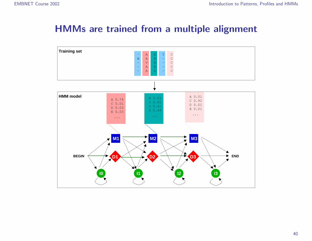
HMMs are trained from a multiple alignment

I2I1

D3D2

M3M2

D1

I3

M1

ENDBEGIN

I0

E 0.44D 0.41C 0.01A 0.01

... ...

C 0.01

E 0.03

A 0.01

W A E - C

D 0.03

- A D T C

C 0.92D 0.01E 0.01

...

- A E - C- A D - C- V E - C

A 0.74HMM model

Training set

40


Match a sequence to a model: find the best path

I3M1I0 M3M2 I2A R A E S P D C I A R A E S P D C I

I3I2

D2

M3

I1

M2

D1 D3BEGIN END

M1

I0

...E 0.44 E 0.01D 0.41 D 0.01

A 0.01C 0.92

...

C 0.01A 0.01

...

E 0.03D 0.03C 0.01A 0.74

41


Algorithms associated with HMMs

. Three important questions can be answered by three algorithms.

. How likely is a given sequence under a given model?

. This is the scoring problem and it can be solved using the Forward algorithm.

. What is the most probable path between states of a model given a sequence?

. This is the alignment problem and it is solved by the Viterbi algorithm.

. How can we learn the HMM parameters given a set of sequences?

. This is the training problem and is solved using the Forward-backward algorithmand the Baum-Welch expectation maximization.

. For details about these algorithms see:

Durbin, Eddy, Mitchison, Krog.Biological Sequence Analysis: Probabilistic Models of Proteins and NucleicAcids.Cambridge University Press, 1998.

42


Hidden Markov Models: Softwares

. HMMER2 is a package to build and use HMMs developed by Sean Eddy(http://hmmer.wustl.edu/).

. Software available in HMMER2:

. hmmbuild to build an HMM model from a multiple alignment;

. hmmalign to align sequences to an HMM model;

. hmmcalibrate to calibrate an HMM model;

. hmmemit to create sequences from an HMM model;

. hmmsearch to search a sequence database with an HMM model;

. hmmpfam to scan a sequence with a database of HMM models;

. ...

. SAM is a similar package developed by Richard Hughey, Kevin Karplus and AndersKrogh (http://www.cse.ucsc.edu/research/compbio/sam.html).

43


The ”Plan 7” architecture of HMMER2

S N B

J

I1 I2 I3

E C T

M3M2M1

D2

M4

D1 D4D3

44


Hidden Markov Models: Conclusions

. Solid thoretical basis in the theory of probabilities.

. Other Advantages and limitations just like generalized profiles.

45


Generalized profiles and HMMs I

. Generalized profiles are equivalent to the ’linear’ HMMs like those of SAMor HMMER2 (they are not equivalent to other HMMs of more complicatedarchitecture).

. The optimal alignment produced by dynamical programming is equivalent to theViterbi path on a HMM.

. There are programs to translate profiles from and into HMMs:

. htop: HMM to profile.

. ptoh: profile to HMM.

46


Generalized profiles and HMMs II

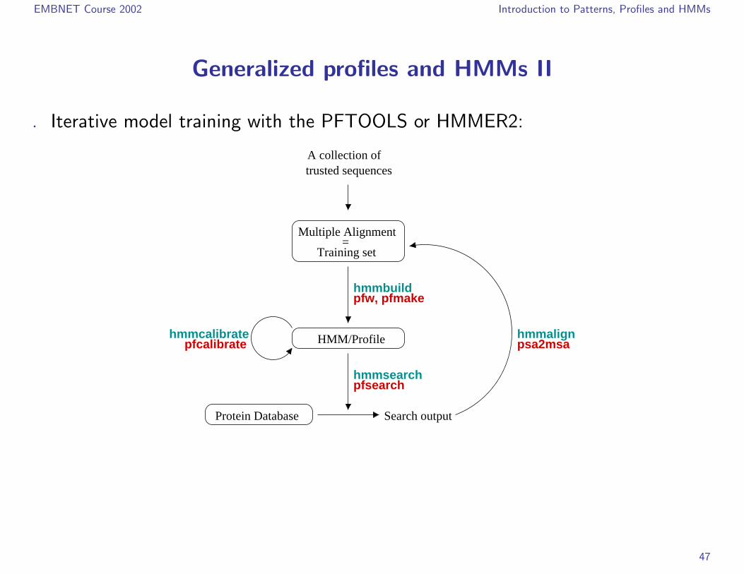
. Iterative model training with the PFTOOLS or HMMER2:

hmmalign

hmmsearchpfsearch

hmmbuild

pfcalibratehmmcalibrate

psa2msa

pfw, pfmake

Multiple Alignment

Training set=

Protein Database

HMM/Profile

Search output

trusted sequencesA collection of

47


Generalized profiles and HMMs III

. HMMs and generalized profiles are very appropriate for the modelling of proteindomains.

. What are protein domains:

. Domains are discrete structural units (25-500 aa).

. Short domains (25-50 aa) are present in multiple copies for structural stability.

. Domains are functional units.

48


PSI-blast I

. PSSM could have simply been improved by the introduction of a position-independent affine gap cost model;

. This is less sophistication than the generalized profiles;

. But it is just this principle that is behind PSI-blast.

. The success and efficiency of PSI-blast has also much to do with:

. the speed of the blast heuristic;

. a particularily efficient algorithm for sequence weighting;

. a very sophisticated statistical treatment of the match scores.

49


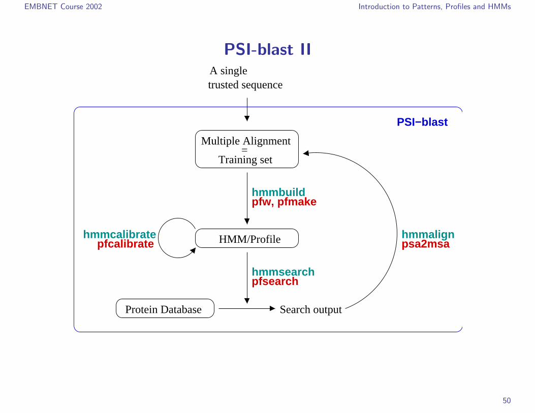
PSI-blast II

hmmalign

hmmsearchpfsearch

hmmbuild

pfcalibratehmmcalibrate

psa2msa

pfw, pfmake

Multiple Alignment

Training set=

Protein Database

HMM/Profile

Search output

A single

PSI−blast

trusted sequence

50


Databases

51


Patterns and PSSM databses

. Patterns database

. Prosite

. WEB access: http://www.expasy.ch/prosite/.

. Contains also profiles.

. Well documented.

. Easy to test new patterns.

. PSSM databases:

. BLOCKS

PRINTS.

. WEB access: http://www.blocks.fhcrc.org/

http://bioinf.man.ac.uk/dbbrowser/PRINTS/.

. Automatically produces PSSMs from families of sequences.

. Easy to scan databases with the produced PSSMs.

52


Protein domain databases

. A non-exhaustive list of protein domain databases:

. Pfam

. http://www.sanger.ac.uk/Pfam.

. Collection of protein domains and families (3071 entries in Pfam release 6.6).

. Uses HMMs (HMMER2).

. Good links to structure, taxonomy.

. PROSITE

. http://www.expasy.ch/prosite.

. Collection of motifs, protein domains, and families (1494 entries in Prosite release

16.51).

. Uses generalized profiles (Pftools) and patterns.

. High quality documentation.

53


Protein domain databases

. A non-exhaustive list of protein domain databases (continued):

. Prints

. http://bioinf.man.ac.uk/dbbrowser/PRINTS.

. Collection of conserved motifs used to characterize a protein.

. Uses fingerprints (conserved motif groups).

. Very good to describe sub-families.

. Release 32.0 of PRINTS contains 1600 entries, encoding 9800 individual motifs.

. ProDom

. http://prodes.toulouse.inra.fr/prodom/doc/prodom.html.

. Collection of protein motifs obtained automatically using PSI-BLAST.

. Very high throughput ... but no annotation.

. ProDom release 2001.2 contains 101957 families (at least 2 sequences per family).

. ...

54


InterPro

. InterPro is an attempt to group a number of protein domain databases:

. Pfam

. PROSITE

. PRINTS

. ProDom

. SMART

. TIGRFAMs

. InterPro tries to have and maintain a high quality annotation.

. Very good accession to examples.

. InterPro web site: http://www.ebi.ac.uk/interpro.

. The database and a stand-alone package (iprscan) are availablefor UNIX platforms to locally run a complete Interpro analysis:ftp://ftp.ebi.ac.uk/pub/databases/interpro.

55


InterPro

. Example of a graphical output:

56


The end

57

Date post:	15-Mar-2020
Category:	Documents
Upload:	others
View:	13 times
Download:	0 times

Introduction to Patterns, Pro les and Hidden Markov...

Documents