Introduction to Phase-Resolving Wave Modeling with FUNWAVE · Introduction to Phase-Resolving Wave...

ERDC/CHL CHETN-I-87 July 2015

Approved for public release; distribution is unlimited.

Introduction to Phase-Resolving Wave

Modeling with FUNWAVE

by Matt Malej, Jane M. Smith, and Gabriela Salgado-Dominguez

PURPOSE: The subject of this note is to delineate the U.S. Army Corps of Engineers (USACE) needs in near-shore processes and evaluate a new phase-resolving numerical wave model for adoption and implementation within Coastal and Hydraulics Laboratory (CHL) numerical strategic framework. An additional consideration is the advancement of the state of the art of the phase-resolving numerical wave models for the USACE. The areas of applicability include near-shore wind-wave propagation, harbor entrances, nonlinear shoaling, runup, overtopping, inundation, tsunamis, and ship waves.

INTRODUCTION: Modeling nonlinear coastal wave processes, such as inundation, wave runup, bore propagation, tsunami propagation, harbor resonance, ship wakes, and infragravity waves, requires efficient and accurate computing of the evolution of highly nonlinear time-dependent, three-dimensional (3D) surface wave fields in complex coastal environments. This is a challenging hydrodynamic problem. Most models commonly used for describing nonlinear surface waves are far from being complete. They rely on ad hoc models for the physical processes involved, such as nonlinear wave-wave interactions, energy dissipation due to wave breaking, or interplay between waves and currents.

An additional complication in modeling coastal waves is that there is a wide range of scales to be resolved. The coupling between various modes and thus the energy transfer between different spatial and temporal scales lacks thorough understanding. Operational phase-averaged wave action balance models suffer from inaccurate prediction of the wave spectrum in shallow water. This is often attributed to incomplete modeling of nonlinear interactions (both resonant and non-resonant). With improvements in the high performance computing (HPC), phase-resolving models are becoming more practical to apply. Their primary area of application thus far has been a shallow-water environment. Boussinesq-type models are especially attractive in these regimes, where weak nonlinearity and low dispersion are prevalent. The USACE has a pressing need for a robust and computationally efficient phase-resolving numerical wave model. It is important that such a model be efficient and developed with HPC application in mind, without the immediate and cyclical need to resort to propriety software packages such as MATLAB.

Statements of need. Statements of need submitted by USACE Districts and discussions with several prominent figures in the Boussinesq-type modeling community (Prof. Patrick Lynett, Prof. Andrew Kennedy, Dr. Zeki Demirbilek) have identified several needs for Boussinesq-type models. These include

• coastal and inland breakwater design (complex geometries) • inundation mapping – overland propagation and runup

Report Documentation Page Form ApprovedOMB No. 0704-0188

Public reporting burden for the collection of information is estimated to average 1 hour per response, including the time for reviewing instructions, searching existing data sources, gathering andmaintaining the data needed, and completing and reviewing the collection of information. Send comments regarding this burden estimate or any other aspect of this collection of information,including suggestions for reducing this burden, to Washington Headquarters Services, Directorate for Information Operations and Reports, 1215 Jefferson Davis Highway, Suite 1204, ArlingtonVA 22202-4302. Respondents should be aware that notwithstanding any other provision of law, no person shall be subject to a penalty for failing to comply with a collection of information if itdoes not display a currently valid OMB control number.

1. REPORT DATE JUL 2015 2. REPORT TYPE

3. DATES COVERED 00-00-2015 to 00-00-2015

4. TITLE AND SUBTITLE Introduction to Phase-Resolving Wave Modeling with FUNWAVE

5a. CONTRACT NUMBER

5b. GRANT NUMBER

5c. PROGRAM ELEMENT NUMBER

6. AUTHOR(S) 5d. PROJECT NUMBER

5e. TASK NUMBER

5f. WORK UNIT NUMBER

7. PERFORMING ORGANIZATION NAME(S) AND ADDRESS(ES) U.S. Army Engineer Research and Development Center,,Vicksburg,,MS

8. PERFORMING ORGANIZATIONREPORT NUMBER

9. SPONSORING/MONITORING AGENCY NAME(S) AND ADDRESS(ES) 10. SPONSOR/MONITOR’S ACRONYM(S)

11. SPONSOR/MONITOR’S REPORT NUMBER(S)

12. DISTRIBUTION/AVAILABILITY STATEMENT Approved for public release; distribution unlimited

13. SUPPLEMENTARY NOTES

14. ABSTRACT The subject of this note is to delineate the U.S. Army Corps of Engineers (USACE) needs in near-shoreprocesses and evaluate a new phase-resolving numerical wave model for adoption and implementationwithin Coastal and Hydraulics Laboratory (CHL) numerical strategic framework. An additionalconsideration is the advancement of the state of the art of the phase-resolving numerical wave models forthe USACE. The areas of applicability include near-shore wind-wave propagation, harbor entrances,nonlinear shoaling, runup, overtopping, inundation, tsunamis, and ship waves.

15. SUBJECT TERMS

16. SECURITY CLASSIFICATION OF: 17. LIMITATION OF ABSTRACT Same as

Report (SAR)

18. NUMBEROF PAGES

25

19a. NAME OFRESPONSIBLE PERSON

a. REPORT unclassified

b. ABSTRACT unclassified

c. THIS PAGE unclassified

Standard Form 298 (Rev. 8-98) Prescribed by ANSI Std Z39-18


2

• bore propagation, waves on reefs • harbor resonance, harbor and marina infrastructure modifications • transient waves (tsunamis, sneaker waves) and ship wakes.

Boussinesq models are essentially shallow-water models with extra dispersive and nonlinear terms. They excel under conditions of weak nonlinearity (long waves in shallow depths). Important processes that need to be modeled by these systems include nonlinear wave-wave interactions, wave-current interactions, wave breaking, nearshore wind-wave propagation, harbor resonance, and nonlinear shoaling.

Unfortunately, Boussinesq models are not presently the best tools for runup and overtopping on near-vertical structures or highly variable bathymetries, due to the removal of the third dimension via the projection and expansion about an arbitrary water depth. Topological changes in the numerical solution of free-surface flows yield some current models obsolete (e.g., Bouss-2D) for near-vertical walls or for fluid-structure interactions. In addition, the associated numerical stability and rates of convergence cannot compete with other more novel numerical schemes (e.g., spectral methods or finite volume/element).

There are many existing Boussinesq models available. Some of these are completely proprietary (e.g., Bouss-2D, DHI models) while others are research codes with little documentation, limited number of active developers, and limited real-world applications. Boussinesq models tend to be very complicated to set up and are not as robust as other types of models. It can be difficult for inexperienced users to apply these codes and to identify problems/errors. In addition, having a one-dimensional (1D) version of the code makes applications generally more accessible and may help promote District applications.

Moreover, due to computational demands of two-dimensional (2D) free-surface wave models, it is imperative that they be implemented for parallel computing. The two Boussinesq-type models that are currently of interest and are written in parallel (MPI – Message Passing Interface) are COULWAVE and FUNWAVE. Both models utilize a MUSCL-TVD (Monotone Upstream-centered Scheme for Conservation Laws – Total Variation Diminishing) finite volume scheme, which is superior to the finite-difference scheme utilized in Bouss-2D. Because COULWAVE and FUNWAVE have largely identical kernels, in the subsequent sections of this report the authors will concentrate exclusively on FUNWAVE.

An additional consideration is that all of the above-mentioned models rely on proprietary software (MATLAB from MathWorks or SMS from AQUAVEO) for grid generation, model initialization, postprocessing, and visualization. While these represent good tool suites for the current needs of the ERDC modeling community, the financial burdens in obtaining licenses on annual basis are an added expense.

Potential improvements of FUNWAVE would include expansion of the user and developer base to create an active implementation group, which is critical for continuous development efforts. Also, an adherence to good software engineering practices such as having a distributed version control system (e.g., Git), writing modular code in higher-level languages/scripts is also important. Finally, it is also vital to be able to dynamically couple phase-resolving models to not only the


3

phase-averaged models but also full-fidelity Navier-Stokes models. These capabilities are currently unexplored in most operational Boussinesq-type models.

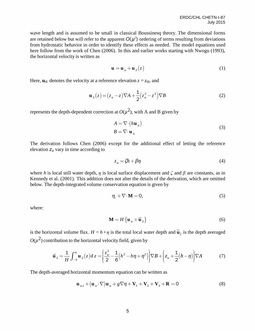
FUNWAVE: Boussinesq wave models have become a useful tool for modeling surface wave transformation from deep water to the swash zone, as well as wave-induced circulation inside the surfzone. Improvements in the range of model applicability have been obtained with respect to classical restrictions to both weak dispersion and weak nonlinearity. Madsen and Sørensen (1992) and Nwogu (1993) demonstrated that the order of approximation in reproducing frequency dispersion effects could be increased using either judicious choices for the form (or reference point) for Taylor series expansions for the vertical structure of dependent variables, or operators effecting a rearrangement of dispersive terms in already developed model equations. These approaches, combined with use either of progressively higher-order truncated series expansions (Gobbi et al. 2000; Agnon et al. 1999) or multiple-level representations (Lynett et al. 2002), have effectively eliminated the restriction of this class of model to relatively shallow water, allowing for their application to the entire shoaling zone or deeper. At the same time, the use of so-called fully nonlinear formulations (e.g., Wei et al. [1995]) and many others) effectively eliminates the restriction to weak nonlinearity by removing the wave height to water depth ratio as a scaling or expansion parameter in the development of approximate governing equations. This approach has improved model applicability in the surf and swash zones particularly, where surface fluctuations are of the order of mean water depth at least and which can represent the total vertical extent of the water column in swash conditions. Representations of dissipative wave-breaking events, which do not naturally arise as weak discontinuous solutions in the dispersive Boussinesq formulation, have been developed usually following an eddy viscosity formulation due to Zelt (1991) and have been shown to be highly effective in describing surf-zone, wave-height decay. The resulting class of models has been shown to be highly effective in modeling wave-averaged surf zone flows over both simple (Chen et al. 2003) and complex bathymetries. Kim et al. (2009) have further extended the formulation to incorporate a consistent representation of boundary layer turbulence effects on vertical flow structure.

Existing approaches to development of numerical implementations for Boussinesq models include a wide range of finite difference, finite volume, or finite element formulations. In this note, there is described the hybrid finite-volume and finite-difference numerical approach for the FUNWAVE model (Kirby et al. 1998), which has been widely used as a public-domain, open-source code since its initial development. FUNWAVE was originally developed using an unstaggered finite difference formulation for spatial derivatives together with an iterated fourth-order Adams-Bashforth-Moulton (ABM) scheme for time-stepping (Wei and Kirby 1995), applied to the fully nonlinear model equations of Wei et al. (1995). In this scheme, spatial differencing is handled using a mixed-order approach, employing fourth-order accurate centered differences for first derivatives and second-order accurate differences for third derivatives. This choice was made in order to move leading order truncation errors to one order higher than the O(µ2) dispersive terms (where µ is ratio of a characteristic water depth to a horizontal length, a dimensionless parameter characterizing frequency dispersion) while maintaining the tridiagonal structure of spatial derivatives within time-derivative terms. This scheme is straightforward to develop and has been widely utilized in other Boussinesq models.

Kennedy et al. (2000) and Chen et al. (2000) describe further aspects of the model system aimed at generalizing it for use in modeling surf zone flows. Breaking is handled using a generalization


4

to two horizontal dimensions of the eddy viscosity model of Zelt (1991). Similar approaches have been used by other Boussinesq model developers, such as Nwogu and Demirbilek (2001), who used a more sophisticated eddy viscosity model in which the eddy viscosity is expressed in terms of turbulent kinetic energy and a length scale. The presence of a moving shoreline in the swash zone is handled using a slot or porous-beach method, in which the entire domain remains wetted using a network of slots at grid resolution that are narrow but which extend down to a depth lower than the minimum expected excursion of the modeled free surface. Several extensions have been made in research versions of the code. Kennedy et al. (2001) improved nonlinear performance of the model by utilizing an adaptive reference level for vertical series expansions, which is allowed to move up and down with local surface fluctuations. Chen et al. (2003) extended the model to include longshore periodic boundary conditions and described its application to modeling long-shore currents on relatively straight coastlines. Shi et al. (2001) generalized the model coordinate system to non-orthogonal curvilinear coordinates. Finally, Chen et al. (2003) and Chen (2006) provided revised model equations which correct deficiencies in the representation of higher order advection terms, leading to a set of model equations that, in the absence of dissipation effects, conserve depth-integrated potential vorticity to O(µ2), consistent with the level of approximation in the model equations.

A number of recently developed Boussinesq-type wave models have used a hybrid method combining the finite-volume and finite-difference TVD-type schemes (Toro 2009) and have shown robust performance of the shock-capturing method in simulating breaking waves and coastal inundation (Tonelli and Petti 2009, 2010; Roeber et al. 2010). The use of the hybrid method, in which the underlying components of the nonlinear shallow water equations (which form the basis of the Boussinesq model equations) are handled using the TVD finite volume method while dispersive terms are implemented using conventional finite differencing, provides a robust framework for modeling of surf zone flows. In particular, wave breaking may be handled entirely by the treatment of weak solutions in the shock-capturing TVD scheme, making the implementation of an explicit formulation for breaking wave dissipation unnecessary. In addition, shoreline movement may be handled quite naturally as part of the Riemann solver underlying the finite volume scheme.

In contrast to previous high-order temporal schemes, which usually require uniform time-stepping, FUNWAVE uses adaptive time-stepping based on a third-order Runge-Kutta method. Spatial derivatives are discretized using a combination of finite-volume and finite-difference methods. A high-order MUSCL reconstruction technique, which is accurate up to the fourth-order, is used in the Riemann solver. The wave-breaking scheme follows the approach of Tonelli and Petti (2009), who used the ability of the nonlinear shallow water equations (NLSWE) with a TVD solver to simulate moving hydraulic jumps. Wave breaking is modeled by switching from Boussinesq to NLSWE at cells where the Froude number exceeds a certain threshold. A wetting-drying scheme is used to model a moving shoreline.

The model was parallelized using the domain decomposition technique. The MPI with nonblocking communication is used for data communication between processors. Additional details on code parallelization is discussed in the subsequent sections.

Formulation. In the present FUNWAVE model, a set of Boussinesq equations are accurate to O(µ2) in dispersive effects. Where µ is a parameter characterizing the ratio of water depth to


5

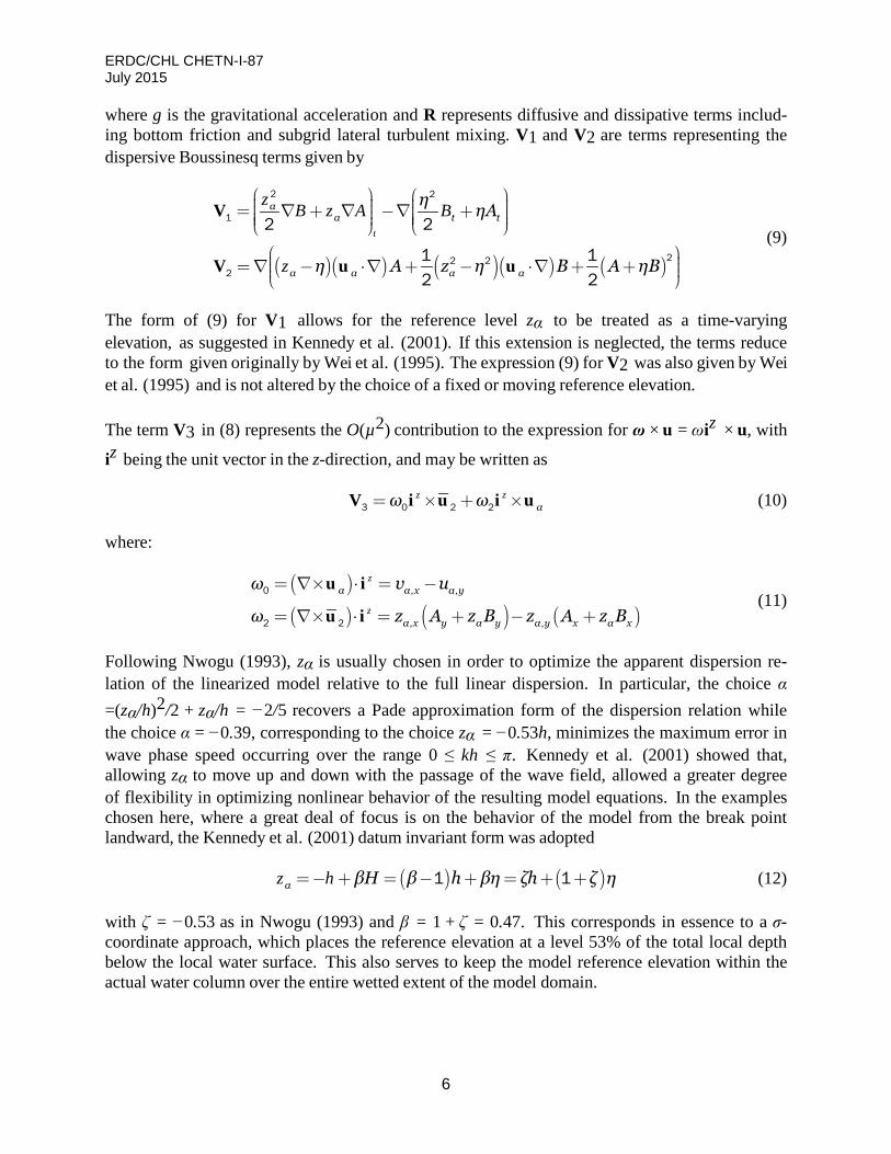
wave length and is assumed to be small in classical Boussinesq theory. The dimensional forms are retained below but will refer to the apparent O(µ2) ordering of terms resulting from deviations from hydrostatic behavior in order to identify these effects as needed. The model equations used here follow from the work of Chen (2006). In this and earlier works starting with Nwogu (1993), the horizontal velocity is written as

α z 2u u u (1)

Here, uα denotes the velocity at a reference elevation z = zα, and

2 22

12

u α αz z z A z z B (2)

represents the depth-dependent correction at O(µ2), with A and B given by

αα

A h

B

u

u (3)

The derivation follows Chen (2006) except for the additional effect of letting the reference elevation zα vary in time according to

αz ζh βη (4)

where h is local still water depth, η is local surface displacement and ζ and β are constants, as in Kennedy et al. (2001). This addition does not alter the details of the derivation, which are omitted below. The depth-integrated volume conservation equation is given by

,tη 0M (5)

where:

αH 2M u u (6)

is the horizontal volume flux. H = h + η is the total local water depth and u2 is the depth averaged

O(µ2) contribution to the horizontal velocity field, given by

2

2 22 2

1 1 12 6 2

u u dη

ααh

zz z h hη η B z h η A

H (7)

The depth-averaged horizontal momentum equation can be written as

,α t α α g η 1 2 3 0u u u V V V R (8)


6

where g is the gravitational acceleration and R represents diffusive and dissipative terms including bottom friction and subgrid lateral turbulent mixing. V1 and V2 are terms representing the dispersive Boussinesq terms given by

αα t t

t

α α α α

z ηB z A B ηA

z η A z η B A ηB

2 2

1

22 22

2 2

1 12 2

V

V u u

(9)

The form of (9) for V1 allows for the reference level zα to be treated as a time-varying elevation, as suggested in Kennedy et al. (2001). If this extension is neglected, the terms reduce to the form given originally by Wei et al. (1995). The expression (9) for V2 was also given by Wei et al. (1995) and is not altered by the choice of a fixed or moving reference elevation.

The term V3 in (8) represents the O(µ2) contribution to the expression for ω × u = ωiz × u, with

iz being the unit vector in the z-direction, and may be written as

z zαω ω 3 0 2 2V i u i u (10)

where:

, ,

, ,

zα α x α y

zα x y α y α y x α x

ω v u

ω z A z B z A z B

0

2 2

u i

u i (11)

Following Nwogu (1993), zα is usually chosen in order to optimize the apparent dispersion relation of the linearized model relative to the full linear dispersion. In particular, the choice α =(zα/h)2/2 + zα/h = −2/5 recovers a Pade approximation form of the dispersion relation while the choice α = −0.39, corresponding to the choice zα = −0.53h, minimizes the maximum error in wave phase speed occurring over the range 0 ≤ kh ≤ π. Kennedy et al. (2001) showed that, allowing zα to move up and down with the passage of the wave field, allowed a greater degree of flexibility in optimizing nonlinear behavior of the resulting model equations. In the examples chosen here, where a great deal of focus is on the behavior of the model from the break point landward, the Kennedy et al. (2001) datum invariant form was adopted

αz h βH β h βη ζh ζ η 11 (12)

with ζ = −0.53 as in Nwogu (1993) and β = 1 + ζ = 0.47. This corresponds in essence to a σ-coordinate approach, which places the reference elevation at a level 53% of the total local depth below the local water surface. This also serves to keep the model reference elevation within the actual water column over the entire wetted extent of the model domain.


7

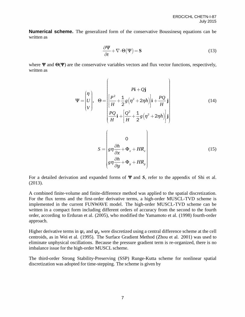
Numerical scheme. The generalized form of the conservative Boussinesq equations can be written as

ΨΘ Ψ

t

S (13)

where Ψ and Θ(Ψ) are the conservative variables vectors and flux vector functions, respectively, written as

Ψ , Θ

P Qη

P PQU g η ηhH H

VPQ Q g η ηhH H

22

22

1 22

1 22

i j

i j

i j

(14)

0

Φ

Φ

x x

y y

hS gη HRxhgη HRy

(15)

For a detailed derivation and expanded forms of Ψ and S, refer to the appendix of Shi et al. (2013).

A combined finite-volume and finite-difference method was applied to the spatial discretization. For the flux terms and the first-order derivative terms, a high-order MUSCL-TVD scheme is implemented in the current FUNWAVE model. The high-order MUSCL-TVD scheme can be written in a compact form including different orders of accuracy from the second to the fourth order, according to Erduran et al. (2005), who modified the Yamamoto et al. (1998) fourth-order approach.

Higher derivative terms in ψx and ψy were discretized using a central difference scheme at the cell centroids, as in Wei et al. (1995). The Surface Gradient Method (Zhou et al. 2001) was used to eliminate unphysical oscillations. Because the pressure gradient term is re-organized, there is no imbalance issue for the high-order MUSCL scheme.

The third-order Strong Stability-Preserving (SSP) Runge-Kutta scheme for nonlinear spatial discretization was adopted for time-stepping. The scheme is given by


8

1 1

2 1 1 2

1 2 2 1

3 14 41 23 3

S

S

S

( ) ( )

( ) ( ) ( ) ( )

( ) ( )

Ψ Ψ ( Θ(Ψ ) )

Ψ Ψ Ψ ( Θ(Ψ ) )

Ψ Ψ Ψ ( Θ(Ψ ) )

n n

n

n n n

t

t

t

(16)

in which Ψn denotes Ψ at time level n. Ψ(1) and Ψ(2) are values at intermediate stages in the Runge-Kutta integration. As Ψ is obtained at each intermediate step, the velocity (u, v) can be solved by a system of tridiagonal matrix equations formed by (13). S needs to be updated using (u, v, η) at the corresponding time step and iterations are needed to achieve convergence.

An adaptive time-step is chosen, following the Courant-Friedrichs-Lewy (CFL) criterion:

min, , , , , ,

min ,min( ) ( )i j i j i j i j i j i j

x yCu g h η v g h η

(17)

where the Courant number and Cmin = 0.5 were used in all validation and verification (V&V) test cases.

The wave breaking scheme follows the approach of Tonelli and Petti (2009), who successfully used the ability of NLSWE with a TVD scheme to model moving hydraulic jumps. Thus, the fully nonlinear Boussinesq equations are switched to NSWE at cells where the Froude number exceeds a certain threshold. The ratio of wave height to total water depth is chosen as the criterion to switch from Boussinesq to NLSWE, with threshold value set to 0.8, as suggested by Tonelli and Petti.

Various boundary conditions including a wall boundary condition, absorbing boundary condition following Kirby et al. (1998), and periodic boundary condition following Chen et al. (2003) have been implemented in the current FUNWAVE model. Implemented wavemakers include Wei and Kirby’s (1999) internal wavemakers for regular waves and irregular waves. For the irregular wavemaker, an extension was made to incorporate an alongshore periodicity into wave generation in order to eliminate a boundary effect on wave simulations. The technique exactly follows the strategy in Chen et al. (2003), who adjusted the distribution of wave directions in each frequency bin to obtain alongshore periodicity. This approach is effective in modeling of breaking wave-induced nearshore circulation such as alongshore currents and rip currents.

Wind effects are modeled using the wind stress forcing proposed by Chen et al. (2004). The wind stress is expressed by

10 10U C U Caw dw

ρR C

ρ (18)

with Cdw = Cd/(h + η), where h + η represent the mean water depth with surface elevation and Cd corresponding to a drag coefficient, C is wave celerity, U is the velocity at a corresponding elevation, and finally, ρa and ρ represent air density and water density, respectively. The wind


9

stress is only applied on wave crests. A free parameter representing a ratio of the forced crest height to maximum surface elevation has also been implemented in the current FUNWAVE model.

Parallelization. In parallelizing the computational model, a domain decomposition technique was used to subdivide the problem into multiple regions and assign each subdomain to a separate process. Each subdomain region contains an overlapping area of ghost cells, three rows deep, as required by the fourth-order MUSCL-TVD scheme. The MPI with nonblocking communication was used to exchange data in the overlapping region between neighboring processors.

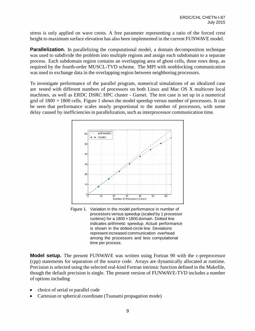
To investigate performance of the parallel program, numerical simulations of an idealized case are tested with different numbers of processors on both Linux and Mac OS X multicore local machines, as well as ERDC DSRC HPC cluster - Garnet. The test case is set up in a numerical grid of 1800 × 1800 cells. Figure 1 shows the model speedup versus number of processors. It can be seen that performance scales nearly proportional to the number of processors, with some delay caused by inefficiencies in parallelization, such as interprocessor communication time.

Figure 1. Variation in the model performance in number of

processors versus speedup (scaled by 1 processor runtime) for a 1800 × 1800 domain. Dotted line indicates arithmetic speedup. Actual performance is shown in the dotted-circle line. Deviations represent increased communication overhead among the processors and less computational time per process.

Model setup. The present FUNWAVE was written using Fortran 90 with the c-preprocessor (cpp) statements for separation of the source code. Arrays are dynamically allocated at runtime. Precision is selected using the selected real-kind Fortran intrinsic function defined in the Makefile, though the default precision is single. The present version of FUNWAVE-TVD includes a number of options including

• choice of serial or parallel code • Cartesian or spherical coordinate (Tsunami propagation mode)


10

• samples • one-way nesting mode • wave breaking index and aging (bubble and foam mode).

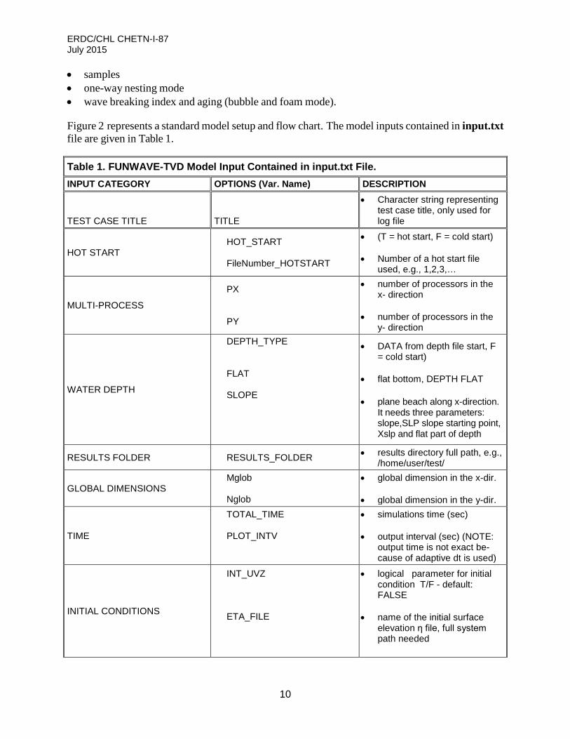
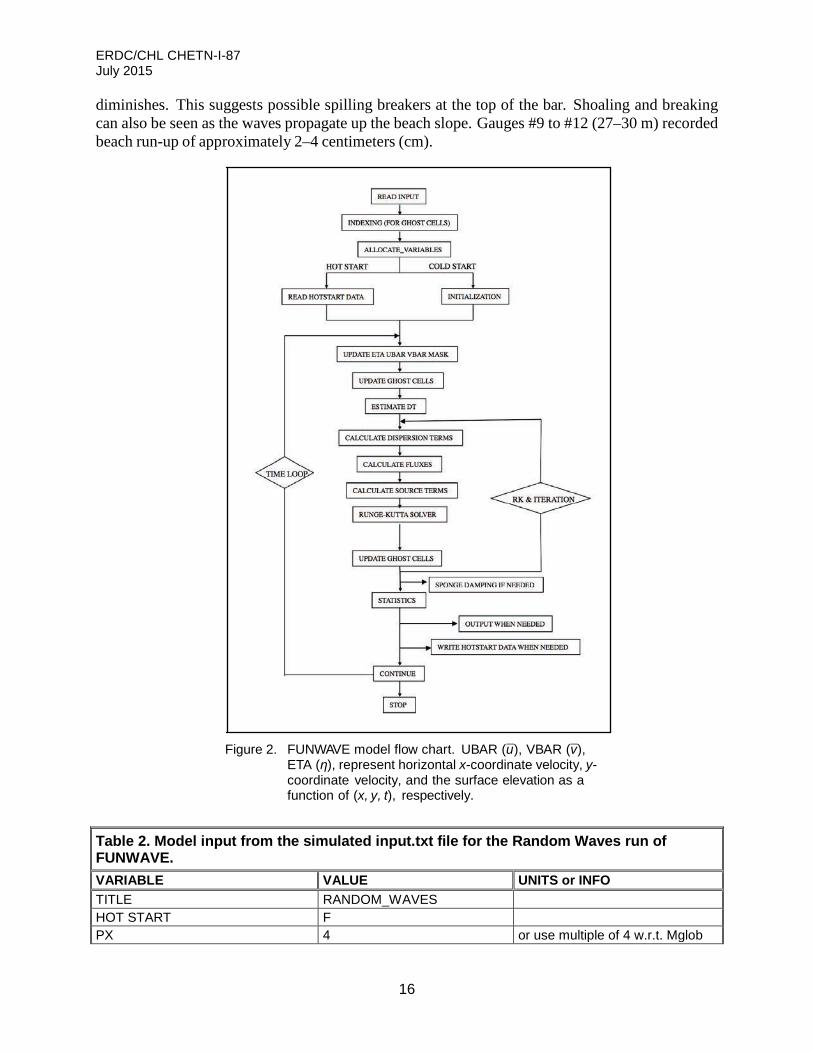
Figure 2 represents a standard model setup and flow chart. The model inputs contained in input.txt file are given in Table 1.

Table 1. FUNWAVE-TVD Model Input Contained in input.txt File. INPUT CATEGORY OPTIONS (Var. Name) DESCRIPTION

TEST CASE TITLE TITLE

• Character string representing test case title, only used for log file

HOT START HOT_START FileNumber_HOTSTART

• (T = hot start, F = cold start)

• Number of a hot start file used, e.g., 1,2,3,…

MULTI-PROCESS

PX PY

• number of processors in the x- direction

• number of processors in the

y- direction

WATER DEPTH

DEPTH_TYPE FLAT SLOPE

• DATA from depth file start, F = cold start)

• flat bottom, DEPTH FLAT • plane beach along x-direction.

It needs three parameters: slope,SLP slope starting point, Xslp and flat part of depth

RESULTS FOLDER RESULTS_FOLDER • results directory full path, e.g., /home/user/test/

GLOBAL DIMENSIONS Mglob Nglob

• global dimension in the x-dir.

• global dimension in the y-dir.

TIME

TOTAL_TIME PLOT_INTV

• simulations time (sec)

• output interval (sec) (NOTE: output time is not exact because of adaptive dt is used)

INITIAL CONDITIONS

INT_UVZ ETA_FILE

• logical parameter for initial condition T/F - default: FALSE

• name of the initial surface

elevation η file, full system path needed


11

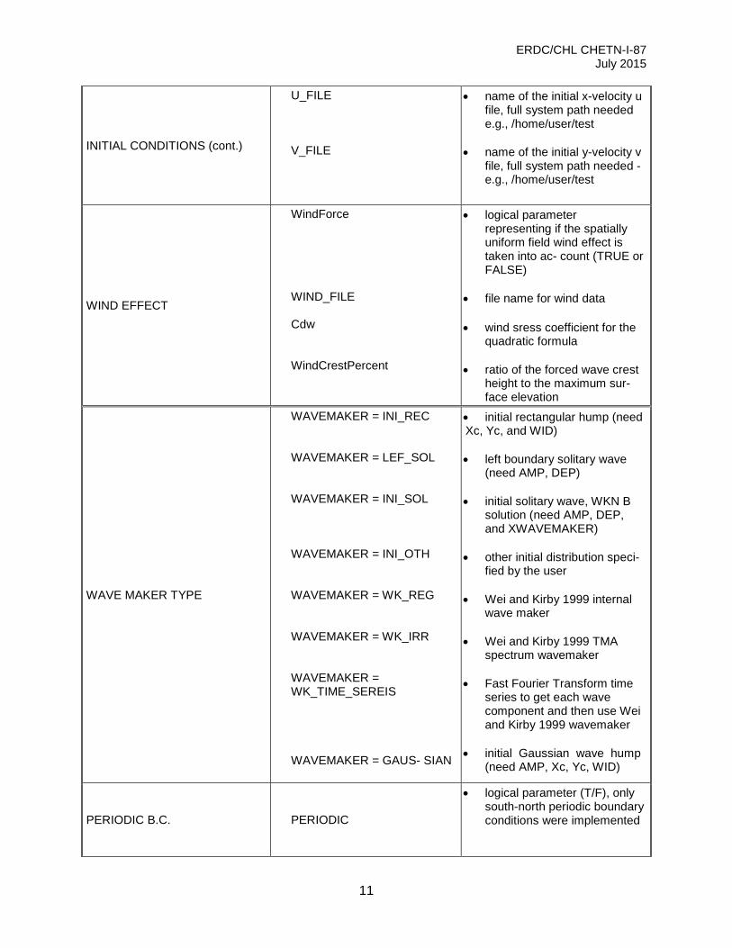
INITIAL CONDITIONS (cont.)

U_FILE V_FILE

• name of the initial x-velocity u file, full system path needed e.g., /home/user/test

• name of the initial y-velocity v

file, full system path needed - e.g., /home/user/test

WIND EFFECT

WindForce WIND_FILE Cdw WindCrestPercent

• logical parameter representing if the spatially uniform field wind effect is taken into ac- count (TRUE or FALSE)

• file name for wind data • wind sress coefficient for the

quadratic formula • ratio of the forced wave crest

height to the maximum surface elevation

WAVE MAKER TYPE

WAVEMAKER = INI_REC WAVEMAKER = LEF_SOL WAVEMAKER = INI_SOL WAVEMAKER = INI_OTH WAVEMAKER = WK_REG WAVEMAKER = WK_IRR WAVEMAKER = WK_TIME_SEREIS WAVEMAKER = GAUS- SIAN

• initial rectangular hump (need Xc, Yc, and WID) • left boundary solitary wave

(need AMP, DEP) • initial solitary wave, WKN B

solution (need AMP, DEP, and XWAVEMAKER)

• other initial distribution speci-

fied by the user • Wei and Kirby 1999 internal

wave maker • Wei and Kirby 1999 TMA

spectrum wavemaker • Fast Fourier Transform time

series to get each wave component and then use Wei and Kirby 1999 wavemaker

• initial Gaussian wave hump

(need AMP, Xc, Yc, WID)

PERIODIC B.C. PERIODIC

• logical parameter (T/F), only south-north periodic boundary conditions were implemented


12

SPONGE LAYER

SPONGE_ON Sponge_west_width Sponge_east_width Sponge_south_width Sponge_north_width R_sponge A_sponge

• logical parameter (T or F)

• width (meters) of west boundary sponge layer

• width (m) of east boundary

• width (m) of south boundary

• width (m) of north boundary

• decay rate (range 0.85 - 0.95)

• maximum damping magn. (∼ 5.0)

OBSTACLES OBSTACLE FILE

• name of obstacle file (1 = water/wet point, 0 = permanent dry point), dimensions are Mglob × Nglob

PHYSICS

DISPERSION Gamma1 Gamma2 Gamma3 Beta_ref SWE_ETA_DEP

• logical parameter (T or F)

• parameter for linear dispersive terms

• parameter for nonlinear dispersive terms

• parameter for linear shallow water equations

• parameter β defined for the reference level (for FUN- WAVE β = −0.531)

• ratio of height/depth for witching from Boussinesq to NSWE (default is 0.80)

BOTTOM FRICTION

FRICTION_MATRIX FRICTION_FILE Cd_fixed

• logical parameter for in/homogenous friction field (T = inhomogeneous, F = homogenous)

• friction data if FRICTION

MATRIX is True, file dimensions should be Mglob × Nglob with the first point as the south-west corner.

• fixed bottom friction coefficient


13

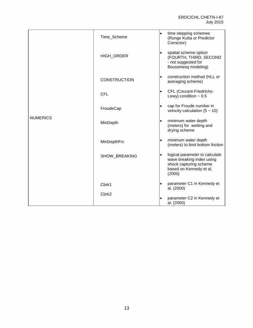
NUMERICS

Time_Scheme HIGH_ORDER CONSTRUCTION CFL FroudeCap MinDepth MinDepthFrc SHOW_BREAKING Cbrk1 Cbrk2

• time stepping schemes (Runge Kutta or Predictor Corrector)

• spatial scheme option

(FOURTH, THIRD, SECOND - not suggested for Boussinesq modeling)

• construction method (HLL or

averaging scheme) • CFL (Courant-Friedrichs-

Lewy) condition ~ 0.5 • cap for Froude number in

velocity calculation (5 ~ 10) • minimum water depth

(meters) for wetting and drying scheme

• minimum water depth (meters) to limit bottom friction

• logical parameter to calculate

wave breaking index using shock capturing scheme based on Kennedy et al. (2000)

• parameter C1 in Kennedy et al. (2000)

• parameter C2 in Kennedy et al. (2000)


14

OUTPUT VARIABLES

NumberStations U V ETA MASK MASK9 SourceX SourceY P Q Fx Fy Gx Gy AGE

• number of station outputs. If NumberStation > 0, need input i, j in STATION_FILE

• logical parameter for x-velocity output u (T or F)

• logical parameter for y-

velocity output v (T or F) • logical parameter for surface

elevation η output (T or F) • logical parameter for wetting-

drying output MASK (T or F) • logical parameter for output

MASK9 – switch from Boussinesq to NSWE (T or F)

• logical parameter for output of

source terms in the x-direction (T or F)


source terms in the y-direction (T or F)


momentum flux in the x- direction (T or F)


momentum flux in the y- direciton (T or F)


numerical flux F in the x- direction (T or F)


numerical flux F in the y- direction (T or F)


numerical flux G in the x- direction (T or F)


numerical flux G in the y- direction (T or F)


breaking age (T or F)


15

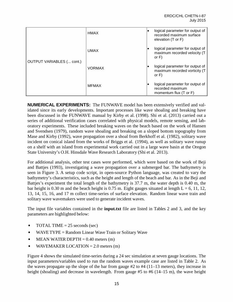
OUTPUT VARIABLES (... cont.)

HMAX UMAX VORMAX MFMAX

• logical parameter for output of recorded maximum surface elevation (T or F)


maximum recorded velocity (T or F)


maximum recorded vorticity (T or F)


recorded maximum momentum flux (T or F)

NUMERICAL EXPERIMENTS: The FUNWAVE model has been extensively verified and validated since its early developments. Important processes like wave shoaling and breaking have been discussed in the FUNWAVE manual by Kirby et al. (1998). Shi et al. (2013) carried out a series of additional verification cases correlated with physical models, remote sensing, and laboratory experiments. These included breaking waves on the beach based on the work of Hansen and Svendsen (1979), random wave shoaling and breaking on a sloped bottom topography from Mase and Kirby (1992), wave propagation over a shoal from Berkhoff et al. (1982), solitary wave incident on conical island from the works of Briggs et al. (1994), as well as solitary wave runup on a shelf with an island from experimental work carried out in a large wave basin at the Oregon State University’s O.H. Hinsdale Wave Research Laboratory (Shi et al. 2013).

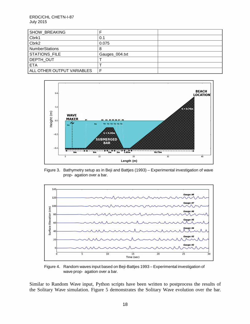
For additional analysis, other test cases were performed, which were based on the work of Beji and Battjes (1993), investigating a wave propagation over a submerged bar. The bathymetry is seen in Figure 3. A setup code script, in open-source Python language, was created to vary the bathymetry’s characteristics, such as the height and length of the beach and bar. As in the Beji and Battjes’s experiment the total length of the bathymetry is 37.7 m, the water depth is 0.40 m, the bar height is 0.30 m and the beach height is 0.75 m. Eight gauges situated at length L = 6, 11, 12, 13, 14, 15, 16, and 17 m collect time-series of surface elevation. Random linear wave train and solitary wave wavemakers were used to generate incident waves.

The input file variables contained in the input.txt file are listed in Tables 2 and 3, and the key parameters are highlighted below:

• TOTAL TIME = 25 seconds (sec) • WAVE TYPE = Random Linear Wave Train or Solitary Wave • MEAN WATER DEPTH = 0.40 meters (m) • WAVEMAKER LOCATION = 2.0 meters (m)

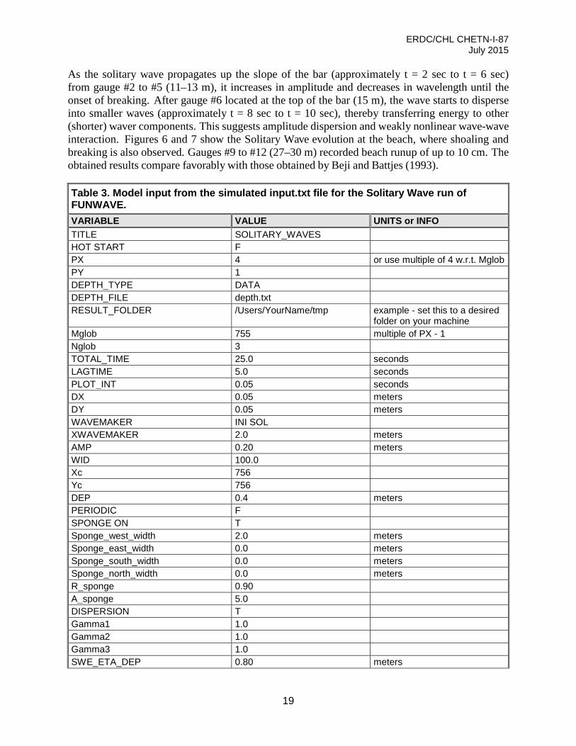
Figure 4 shows the simulated time-series during a 24 sec simulation at seven gauge locations. The input parameters/variables used to run the random waves example case are listed in Table 2. As the waves propagate up the slope of the bar from gauge #2 to #4 (11–13 meters), they increase in height (shoaling) and decrease in wavelength. From gauge #5 to #6 (14–15 m), the wave height


16

diminishes. This suggests possible spilling breakers at the top of the bar. Shoaling and breaking can also be seen as the waves propagate up the beach slope. Gauges #9 to #12 (27–30 m) recorded beach run-up of approximately 2–4 centimeters (cm).

Figure 2. FUNWAVE model flow chart. UBAR (u), VBAR (v),

ETA (η), represent horizontal x-coordinate velocity, y-coordinate velocity, and the surface elevation as a function of (x, y, t), respectively.

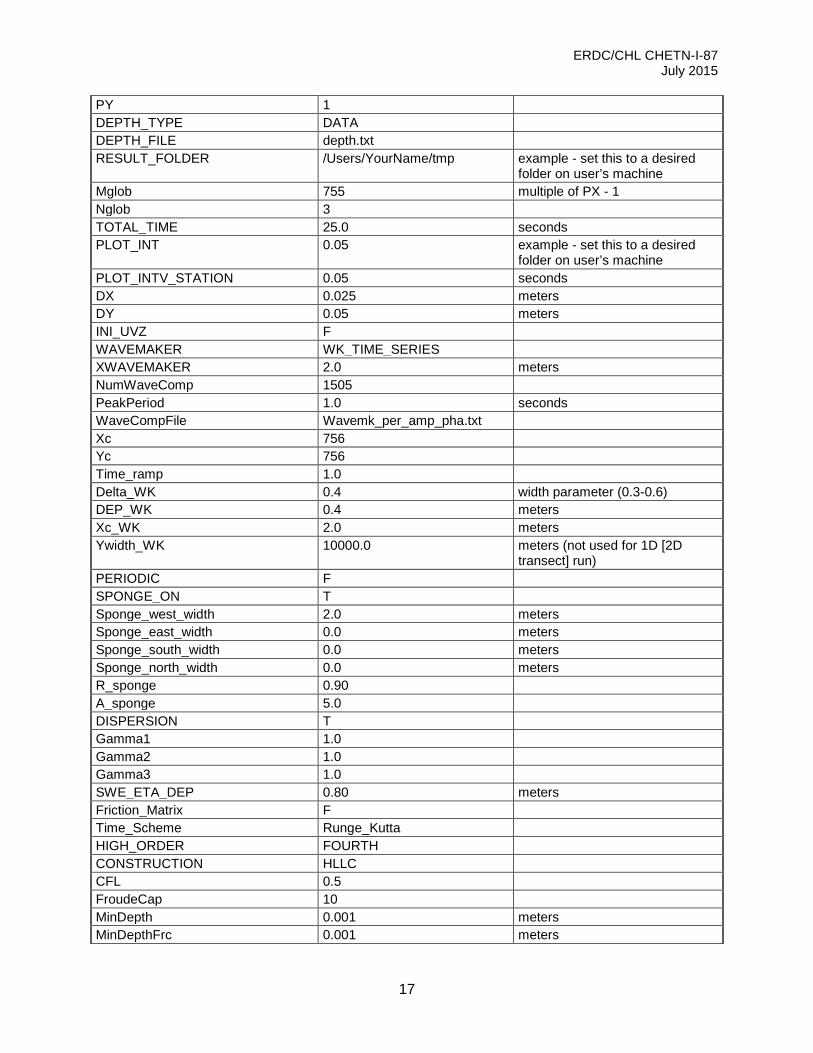
Table 2. Model input from the simulated input.txt file for the Random Waves run of FUNWAVE. VARIABLE VALUE UNITS or INFO TITLE RANDOM_WAVES HOT START F PX 4 or use multiple of 4 w.r.t. Mglob


17

PY 1 DEPTH_TYPE DATA DEPTH_FILE depth.txt RESULT_FOLDER /Users/YourName/tmp example - set this to a desired

folder on user’s machine Mglob 755 multiple of PX - 1 Nglob 3 TOTAL_TIME 25.0 seconds PLOT_INT 0.05 example - set this to a desired

folder on user’s machine PLOT_INTV_STATION 0.05 seconds DX 0.025 meters DY 0.05 meters INI_UVZ F WAVEMAKER WK_TIME_SERIES XWAVEMAKER 2.0 meters NumWaveComp 1505 PeakPeriod 1.0 seconds WaveCompFile Wavemk_per_amp_pha.txt Xc 756 Yc 756 Time_ramp 1.0 Delta_WK 0.4 width parameter (0.3-0.6) DEP_WK 0.4 meters Xc_WK 2.0 meters Ywidth_WK 10000.0 meters (not used for 1D [2D

transect] run) PERIODIC F SPONGE_ON T Sponge_west_width 2.0 meters Sponge_east_width 0.0 meters Sponge_south_width 0.0 meters Sponge_north_width 0.0 meters R_sponge 0.90 A_sponge 5.0 DISPERSION T Gamma1 1.0 Gamma2 1.0 Gamma3 1.0 SWE_ETA_DEP 0.80 meters Friction_Matrix F Time_Scheme Runge_Kutta HIGH_ORDER FOURTH CONSTRUCTION HLLC CFL 0.5 FroudeCap 10 MinDepth 0.001 meters MinDepthFrc 0.001 meters


18

SHOW_BREAKING F Cbrk1 0.1 Cbrk2 0.075 NumberStations 8 STATIONS_FILE Gauges_004.txt DEPTH_OUT T ETA T ALL OTHER OUTPUT VARIABLES F

Figure 3. Bathymetry setup as in Beji and Battjes (1993) – Experimental investigation of wave

propagation over a bar.

Figure 4. Random waves input based on Beji-Battjes 1993 – Experimental investigation of

wave propagation over a bar.

Similar to Random Wave input, Python scripts have been written to postprocess the results of the Solitary Wave simulation. Figure 5 demonstrates the Solitary Wave evolution over the bar.

Length (m)


19

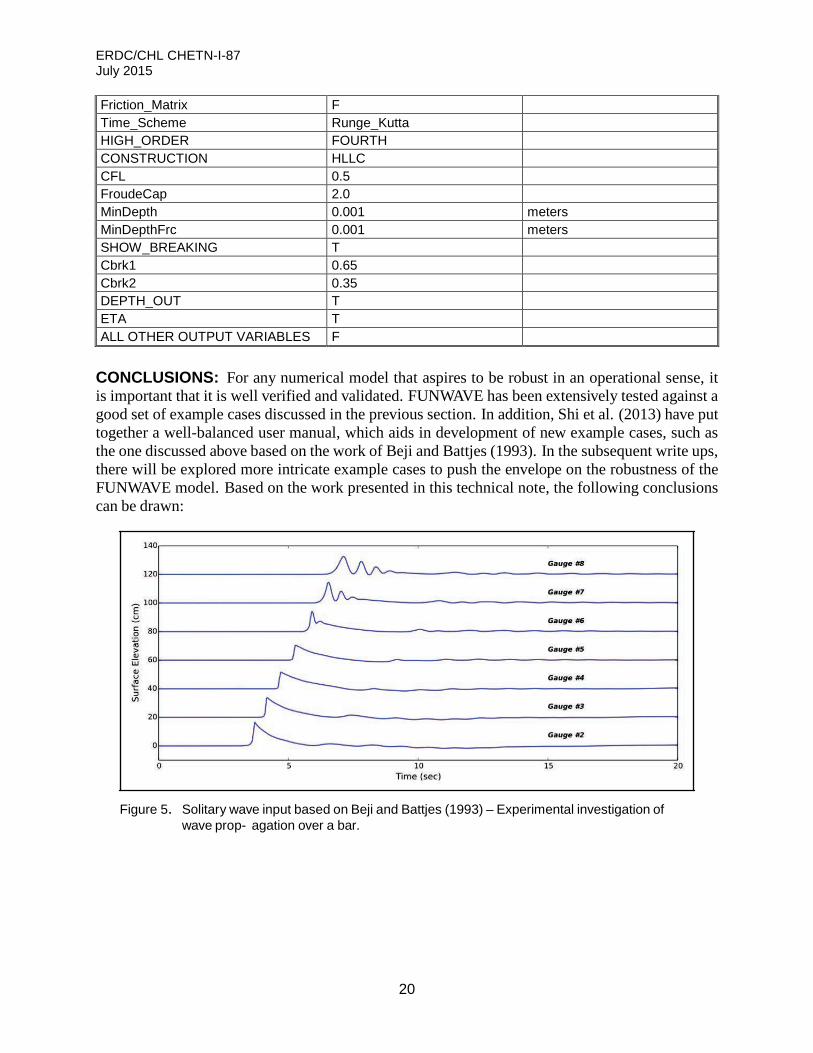
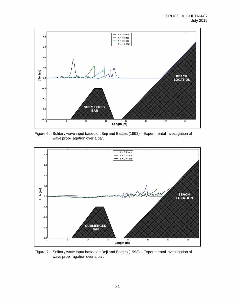
As the solitary wave propagates up the slope of the bar (approximately t = 2 sec to t = 6 sec) from gauge #2 to #5 (11–13 m), it increases in amplitude and decreases in wavelength until the onset of breaking. After gauge #6 located at the top of the bar (15 m), the wave starts to disperse into smaller waves (approximately t = 8 sec to t = 10 sec), thereby transferring energy to other (shorter) waver components. This suggests amplitude dispersion and weakly nonlinear wave-wave interaction. Figures 6 and 7 show the Solitary Wave evolution at the beach, where shoaling and breaking is also observed. Gauges #9 to #12 (27–30 m) recorded beach runup of up to 10 cm. The obtained results compare favorably with those obtained by Beji and Battjes (1993).

Table 3. Model input from the simulated input.txt file for the Solitary Wave run of FUNWAVE. VARIABLE VALUE UNITS or INFO TITLE SOLITARY_WAVES HOT START F PX 4 or use multiple of 4 w.r.t. Mglob PY 1 DEPTH_TYPE DATA DEPTH_FILE depth.txt RESULT_FOLDER /Users/YourName/tmp example - set this to a desired

folder on your machine Mglob 755 multiple of PX - 1 Nglob 3 TOTAL_TIME 25.0 seconds LAGTIME 5.0 seconds PLOT_INT 0.05 seconds DX 0.05 meters DY 0.05 meters WAVEMAKER INI SOL XWAVEMAKER 2.0 meters AMP 0.20 meters WID 100.0 Xc 756 Yc 756 DEP 0.4 meters PERIODIC F SPONGE ON T Sponge_west_width 2.0 meters Sponge_east_width 0.0 meters Sponge_south_width 0.0 meters Sponge_north_width 0.0 meters R_sponge 0.90 A_sponge 5.0 DISPERSION T Gamma1 1.0 Gamma2 1.0 Gamma3 1.0 SWE_ETA_DEP 0.80 meters


20

Friction_Matrix F Time_Scheme Runge_Kutta HIGH_ORDER FOURTH CONSTRUCTION HLLC CFL 0.5 FroudeCap 2.0 MinDepth 0.001 meters MinDepthFrc 0.001 meters SHOW_BREAKING T Cbrk1 0.65 Cbrk2 0.35 DEPTH_OUT T ETA T ALL OTHER OUTPUT VARIABLES F

CONCLUSIONS: For any numerical model that aspires to be robust in an operational sense, it is important that it is well verified and validated. FUNWAVE has been extensively tested against a good set of example cases discussed in the previous section. In addition, Shi et al. (2013) have put together a well-balanced user manual, which aids in development of new example cases, such as the one discussed above based on the work of Beji and Battjes (1993). In the subsequent write ups, there will be explored more intricate example cases to push the envelope on the robustness of the FUNWAVE model. Based on the work presented in this technical note, the following conclusions can be drawn:

Figure 5. Solitary wave input based on Beji and Battjes (1993) – Experimental investigation of



21






22

• The FUNWAVE Boussinesq-type, phase-resolving wave model performs qualitatively well in relatively shallow water environments, where weak nonlinearity and low dispersion are prevalent. In particular, when analyzing random and solitary wave propagation over the bar, it replicates the contrasted work rather well (Beji and Battjes 1993) and produces convincing qualitative results.

• In the identified statements of needs, the FUNWAVE model excels in the cases of runup with overtopping and can be of direct use for inundation mapping work. However, it is not ideal for nearly vertical walls due to removal of the third dimension (canonical variables like the surface elevation ζ and velocity potential φ are projected onto and expanded about a fixed depth).

• Its open-source code framework allows for greater user base and development team while being in line with the CHL numerical modeling strategy.

• The model is written in a low-level language (Fortran90), with parallel (MPI) implementation, albeit the parallelization has to be optimized to allow for various combinations of work-load distribution in the dominate and transverse direction. Meaning, currently FUN- WAVE requires that each process contains a full row of the transverse direction data and that the discretization (Mglob) be an exact multiple of the processes (PX).

• Additional items for future considerations are deployability (less platform dependence) and friendly user interface to allow for widespread use of the product, without relying on a suite of tools working seamlessly on every machine. The authors are exploring the use of IPython Notebooks to allow users to connect to remote servers and run their desired example cases in serial or in parallel on a remote cluster.

• Also, it is equally important to develop a nonproprietary suite of setup and postprocessing tools. There have been developed initial scripts for the test cases discussed above in an opensource Python language and its extension modules.

• In addition, input and output need to be standardized and allow for more robust data encapsulation. It is recommended that FUNWAVE adopts XDMF data format for its output.

• A use of distributed version control system to aid in code development is a necessity for any evolving code base, and there has already been an investment into Git through Github in order to adhere to proper software carpentry practices.

• Finally, it is imperative that model applicability guidance be created and distributed with any operational code release. A matrix/table of model use recommendations is needed for the USACE applications so that standard model use does not require an expert to set up and run the code or that the model is not inadvertently being applied in wrong scenarios that cannot be resolved by FUNWAVE.

ADDITIONAL INFORMATION: This CHETN is a product of the A Boussinesq-type Wave Modeling Work Unit of the Flood and Coastal Research Program being conducted at the U.S. Army Engineer Research and Development Center, Coastal and Hydraulics Laboratory. Questions about this technical note can be addressed to Dr. Matt Malej (Voice: 601-634-3742; email: [email protected]). For information about the Flood and Coastal Research Program, please contact the Flood and Coastal Program Manager, Dr. Cary A. Talbot (Voice: 601- 634-2625; email: [email protected]). This technical note should be cited as follows:


23

Malej, M., Smith J. M., and G. Salgado-Dominguez. 2015. Introduction to phase-resolving wave modeling with FUNWAVE. ERDC/CHL CHETN-I-87. Vicksburg, MS: U.S. Army Engineer Research and Development Center.

REFERENCES

Agnon, Y., Madsen, P. A., and H. A. Schaffer. 1999. A new approach to high-order Boussinesq models. Journal of Fluid Mechanics 399:319–333.

Beji, S., and J. A. Battjes. 1993. Experimental investigation of wave propagation over a bar. Coastal Engineering 19:151–162. Amsterdam: Elsevier Science Publishers B.V.

Berkhoff, J. C. W., N. Booy, and A. C. Radder. 1982. Verification of numerical wave propagation models for simple harmonic linear water waves. Coastal Engineering 6:255–279.

Briggs, M. J., C. E. Synolakis and G. S. Harkins. 1994. Tsumani run-up on conical island. In Proceedings of Waves-Physical and Numerical Modeling. International Association for Hydraulic Research, 446–455, Delft, The Netherlands.

Chen, Q., J. T. Kirby, R. A. Dalrymple, A. B. Kennedy, and A. Chawla. 2000. Boussinesq modeling of wave transformation, breaking and runup. II: 2D. Journal of Waterway, Port, Coastal and Ocean Engineering 126:48–56.

Chen, Q., J. T. Kirby, R. A. Dalrymple, F. Shi, and E. B. Thornton. 2003. Boussinesq modeling of longshore currents. Journal of Geophysical Research 108(C11):3362.

Chen, Q., J. M. Kaihatu, and P. A. Hwang. 2004 Incorporation of wind effects into Boussinesq wave models. Journal of Waterway, Port, Coastal and Ocean Engineering 130:312–321.

Chen, Q. 2006. Fully nonlinear Boussinesq-type equations for waves and currents over porous beds. Journal of Engineering Mechanics 132 (2):220–230.

Erduran, K. S., S. Ilic, and V. Kutija. 2005. Hybrid finite-volume finite-difference scheme for the solution of Boussinesq equations. International Journal of Numerical Methods and Fluids 49:1213–1232.

Gobbi, M. F., J. T. Kirby, and G. Wei. 2000. A fully nonlinear Boussinesq model for surface waves. II. Extension to O(kh4). Journal of Fluid Mechanics 405:181–210.

Hansen, J. B, and and I. A. Svendsen. 1979. Regular waves in shoaling water: Experimental data. Tech. Rep. ISVA Series 21. Denmark: Institute of Hydrodynamics and Hydraulic Engineering, Technical University of Denmark.

Kim, D. H., P. J. Lynett, and S. A. Socolofsky. 2009. A depth-integrated model for weakly dispersive, turbulent, and rotational fluid flows. Ocean Modeling 27:198–214.

Kennedy, A. B., Q. Chen, J. T. Kirby, and R. A. Dalrymple. 2000. Boussinesq modeling of wave transformation, breaking and runup. I: 1D. Journal of Waterway, Port, Coastal and Ocean Engineering 12:39–47.

Kennedy, A. B., J. T. Kirby, Q. Chen, and R. A. Dalrymple. 2001. Boussinesq-type equations with improved nonlinear performance. Wave Motion 33:225–243.

Kirby, J. T., G. Wei, Q. Chen, A. B. Kennedy, and R. A. Dalrymple. 1998. FUNWAVE 1.0, Fully nonlinear Boussinesq wave model. Documentation and users manual. Report CACR-98-06. Newark, DE: Cen- ter for Applied Coastal Research, Department of Civil and Environmental Engineering, University of Delaware.

Lynett, P. J., T.-R. Wu, and P. L.-F. Liu. 2002 Modeling wave runup with depth-integrated equations. Coastal Engineering 46:89–107.

Madsen, P. A., and O. R. Sørensen. 1992. A new form of the Boussinesq equations with improved linear dispersion characteristics. Part 2. A slowly-varying bathymetry. Coastal Engineering 18(3-4):183–204.


24

Mase, H., and J. T. Kirby. 1992. Hybrid frequency-domain KdV equation for random wave transformation. In Proceedings of 23rd International Conference Coastal Engineering, ASCE, New York, 474–487.

Nwogu, O. 1993. An alternative form of the Boussinesq equations for nearshore wave propagation. Journal of Waterway, Port, Coastal, and Ocean Engineering 119(6):618–638.

Nwogu, O., and Z. Demirbilek. 2001. BOUSS-2D: A Boussinesq wave model for coastal regions and harbors. ERDC/CHL TR-01-25. Vicksburg, MS: U.S. Army Corps of Engineers Research and Devel- opment Center.

Roeber, V., K. F. Cheung, and M. H. Kobayashi. 2010. Shock-capturing Boussinesq-type model for nearshore wave processes. Coastal Engineering 57:407–423.

Shi, F., R. A. Dalrymple, J. T. Kirby, Q. Chen, and A. Kennedy. 2001. A fully nonlinear Boussinesq model in generalized curvilinear coordinates. Coastal Engineering 42:337–358.

Shi, F., B. Tehranirad, J. T. Kirby, J. C. Harris, and S. Grilli. 2013. FUNWAVE-TVD: Fully nonlinear Boussinesq wave model with TVD solver documentation and user’s manual. Research Report NO. CACR-11-04. Newark, DE: Center of Applied Coastal Research, University of Delaware.

Tonelli, M., and M. Petti. 2009. Hybrid finite volume - finite difference scheme for 2DH improved Boussi- nesq equations. Coastal Engineering 56:609–620.

Tonelli, M., and M. Petti. 2010. Finite volume scheme for the solution of 2D extended Boussinesq equations in the surf zone. Ocean Engineering 37:567–582.

Toro, E. F. 2009. Riemann solvers and numerical methods for fluid dynamics: a practical introduction. 3rd edition. New York: Springer.

Wei, G., and J. T. Kirby. 1995. A time-dependent numerical code for extended Boussinesq equations.

Journal of Waterway, Port, Coastal and Ocean Engineering 120:251–261.

Wei, G., J. T. Kirby, S. T. Grilli, and R. Subramanya. 1995. A fully nonlinear Boussinesq model for surface waves: Part I. Highly nonlinear unsteady waves. Journal of Fluid Mechanics 294:7192.

Yamamoto, S., S. Kano, and H. Daiguji. 1998. An efficient CFD approach for simulating un-steady hyper- sonic shock-shock interference flows. Computers and Fluids 27(56):571–580.

Zelt, J. A. 1991. The runup of nonbreaking and breaking solitary waves. Coastal Engineering 15:205–246.

Zhou, J. G., D. M. Causon, C. G. Mingham, and D. M. Ingram. 2001. The surface gradient method for the treatment of source terms in the shallow-water equations. Journal of Computational Physics 168:1–25.

NOTE: The contents of this technical note are not to be used for advertising, publication, or promotional purposes. Citation of trade names does not constitute an official endorsement or approval of the use of such products.

Date post:	15-Apr-2018
Category:	Documents
Upload:	vanliem
View:	217 times
Download:	2 times

Introduction to Phase-Resolving Wave Modeling with FUNWAVE · Introduction to Phase-Resolving Wave...

Documents