Introduction to Probability, Selected Textbook Summary ... · 6 From Introduction to Probability,...

Introduction to Probability

SECOND EDITION

Dimitri P. Bertsekas and John N. Tsitsiklis

Massachusetts Institute of Technology

Selected Summary Material – All Rights Reserved

WWW site for book information and orders

http://www.athenasc.com

Athena Scientific, Belmont, Massachusetts

1

http://www.athenasc.com

1

Sample Space and

Probability

Excerpts from Introduction to Probability: Second Edition

by Dimitri P. Bertsekas and John N. Tsitsiklis ©c


Contents

1.1. Sets . . . . . . . . . . . . . . . . . . . . . . . . . . . p. 31.2. Probabilistic Models . . . . . . . . . . . . . . . . . . . . p. 61.3. Conditional Probability . . . . . . . . . . . . . . . . . p. 181.4. Total Probability Theorem and Bayes’ Rule . . . . . . . . p. 281.5. Independence . . . . . . . . . . . . . . . . . . . . . . p. 341.6. Counting . . . . . . . . . . . . . . . . . . . . . . . p. 441.7. Summary and Discussion . . . . . . . . . . . . . . . . p. 51

Problems . . . . . . . . . . . . . . . . . . . . . . . . p. 53

1

2 From Introduction to Probability, by Bertsekas and Tsitsiklis Chap. 1

1.1 SETS

1.2 PROBABILISTIC MODELS

Elements of a Probabilistic Model

• The sample space Ω, which is the set of all possible outcomes of anexperiment.

• The probability law, which assigns to a set A of possible outcomes(also called an event) a nonnegative number P(A) (called the proba-bility of A) that encodes our knowledge or belief about the collective“likelihood” of the elements of A. The probability law must satisfycertain properties to be introduced shortly.

Probability Axioms

1. (Nonnegativity) P(A) ≥ 0, for every event A.

2. (Additivity) If A and B are two disjoint events, then the probabilityof their union satisfies

P(A ∪B) = P(A) +P(B).

More generally, if the sample space has an infinite number of elementsand A1, A2, . . . is a sequence of disjoint events, then the probability oftheir union satisfies

P(A1 ∪A2 ∪ · · ·) = P(A1) +P(A2) + · · · .

3. (Normalization) The probability of the entire sample space Ω isequal to 1, that is, P(Ω) = 1.

Sec. 1.2 Probabilistic Models 3

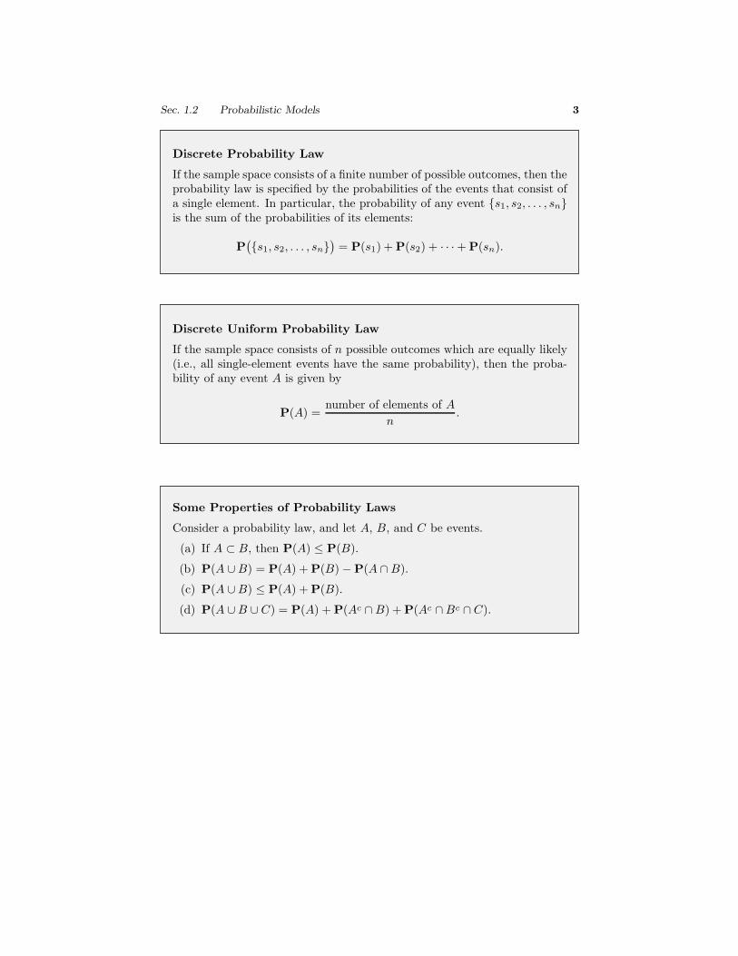
Discrete Probability Law

If the sample space consists of a finite number of possible outcomes, then theprobability law is specified by the probabilities of the events that consist ofa single element. In particular, the probability of any event s1, s2, . . . , snis the sum of the probabilities of its elements:

P(

s1, s2, . . . , sn)

= P(s1) +P(s2) + · · ·+P(sn).

Discrete Uniform Probability Law

If the sample space consists of n possible outcomes which are equally likely(i.e., all single-element events have the same probability), then the proba-bility of any event A is given by

P(A) =number of elements of A

n.

Some Properties of Probability Laws

Consider a probability law, and let A, B, and C be events.

(a) If A ⊂ B, then P(A) ≤ P(B).

(b) P(A ∪B) = P(A) +P(B) −P(A ∩B).

(c) P(A ∪B) ≤ P(A) +P(B).

(d) P(A ∪B ∪ C) = P(A) +P(Ac ∩B) +P(Ac ∩Bc ∩ C).


1.3 CONDITIONAL PROBABILITY

Properties of Conditional Probability

• The conditional probability of an event A, given an event B withP(B) > 0, is defined by

P(AP(A |B) =

∩B),

P(B)

and specifies a new (conditional) probability law on the same samplespace Ω. In particular, all properties of probability laws remain validfor conditional probability laws.

• Conditional probabilities can also be viewed as a probability law on anew universe B, because all of the conditional probability is concen-trated on B.

• If the possible outcomes are finitely many and equally likely, then

number of elements of AP(A |B) =

∩B.

number of elements of B

1.4 TOTAL PROBABILITY THEOREM AND BAYES’ RULE

Total Probability Theorem

Let A1, . . . , An be disjoint events that form a partition of the sample space(each possible outcome is included in exactly one of the events A1, . . . , An)and assume that P(Ai) > 0, for all i. Then, for any event B, we have

P(B) = P(A1 ∩B) + · · ·+P(An ∩B)

= P(A1)P(B |A1) + · · ·+P(An)P(B |An).

Sec. 1.5 Independence 5

1.5 INDEPENDENCE

Independence

• Two events A and B are said to be independent if

P(A ∩B) = P(A)P(B).

If in addition, P(B) > 0, independence is equivalent to the condition

P(A |B) = P(A).

• If A and B are independent, so are A and Bc.

• Two events A and B are said to be conditionally independent,given another event C with P(C) > 0, if

P(A ∩B |C) = P(A |C)P(B |C).

If in addition, P(B ∩ C) > 0, conditional independence is equivalentto the condition

P(A |B ∩ C) = P(A |C).

• Independence does not imply conditional independence, and vice versa.

Definition of Independence of Several Events

We say that the events A1, A2, . . . , An are independent if

P

(

⋂

i∈S

Ai

)

=∏

i∈S

P(Ai), for every subset S of 1, 2, . . . , n.


1.6 COUNTING

The Counting Principle

Consider a process that consists of r stages. Suppose that:

(a) There are n1 possible results at the first stage.

(b) For every possible result at the first stage, there are n2 possible resultsat the second stage.

(c) More generally, for any sequence of possible results at the first i − 1stages, there are ni possible results at the ith stage.

Then, the total number of possible results of the r-stage process is

n1n2 · · ·nr.

Summary of Counting Results

• Permutations of n objects: n!.

• k-permutations of n objects: n!/(n− k)!.

n n!• Combinations of k out of n objects:

(

k

)

= .k! (n− k)!

• Partitions of n objects into r groups, with the ith group having ni

objects:(

n)

n!= .

n1, n2, . . . , nr n1!n2! · · ·nr!

1.7 SUMMARY AND DISCUSSION

2

Discrete Random Variables

Excerpts from Introduction to Probability: Second Editio



n

Contents

2.1. Basic Concepts . . . . . . . . . . . . . . . . . . . . . p. 722.2. Probability Mass Functions . . . . . . . . . . . . . . . p. 742.3. Functions of Random Variables . . . . . . . . . . . . . . p. 802.4. Expectation, Mean, and Variance . . . . . . . . . . . . . p. 812.5. Joint PMFs of Multiple Random Variables . . . . . . . . . p. 922.6. Conditioning . . . . . . . . . . . . . . . . . . . . . . p. 972.7. Independence . . . . . . . . . . . . . . . . . . . . . . p. 1092.8. Summary and Discussion . . . . . . . . . . . . . . . . p. 115

Problems . . . . . . . . . . . . . . . . . . . . . . . . p. 119

7


2.1 BASIC CONCEPTS

Main Concepts Related to Random Variables

Starting with a probabilistic model of an experiment:

• A random variable is a real-valued function of the outcome of theexperiment.

• A function of a random variable defines another random variable.

• We can associate with each random variable certain “averages” of in-terest, such as the mean and the variance.

• A random variable can be conditioned on an event or on anotherrandom variable.

• There is a notion of independence of a random variable from anevent or from another random variable.

Concepts Related to Discrete Random Variables

Starting with a probabilistic model of an experiment:

• A discrete random variable is a real-valued function of the outcomeof the experiment that can take a finite or countably infinite numberof values.

• A discrete random variable has an associated probability mass func-tion (PMF), which gives the probability of each numerical value thatthe random variable can take.

• A function of a discrete random variable defines another discreterandom variable, whose PMF can be obtained from the PMF of theoriginal random variable.

Sec. 2.4 Expectation, Mean, and Variance 9

2.2 PROBABILITY MASS FUNCTIONS

Calculation of the PMF of a Random Variable X

For each possible value x of X :

1. Collect all the possible outcomes that give rise to the event X = x.2. Add their probabilities to obtain pX(x).

2.3 FUNCTIONS OF RANDOM VARIABLES

2.4 EXPECTATION, MEAN, AND VARIANCE

Expectation

We define the expected value (also called the expectation or the mean)of a random variable X , with PMF pX , by

E[X ] =∑

x

xpX(x).

Expected Value Rule for Functions of Random Variables

Let X be a random variable with PMF pX , and let g(X) be a function ofX . Then, the expected value of the random variable g(X) is given by

E[

g(X)]

=∑

x

g(x)pX(x).


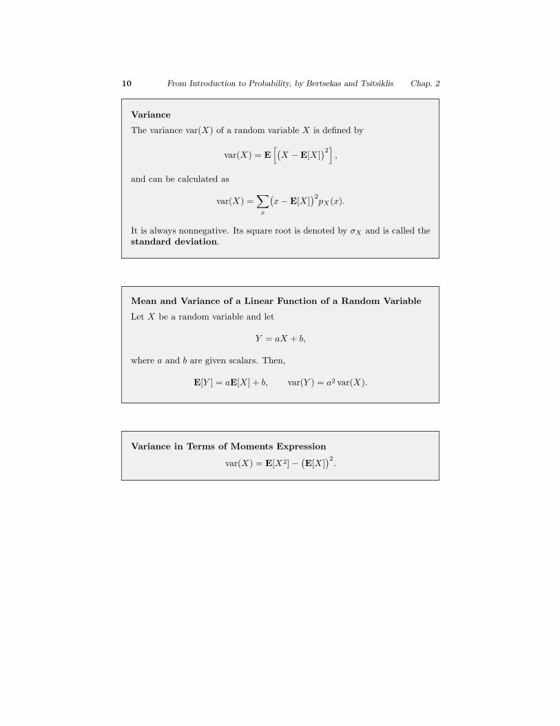
Variance

The variance var(X) of a random variable X is defined by

var(X) = E[

(

X −E[X ])2]

,

and can be calculated as

var(X) =∑

x

(

x−E[X ])2pX(x).

It is always nonnegative. Its square root is denoted by σX and is called thestandard deviation.

Mean and Variance of a Linear Function of a Random Variable

Let X be a random variable and let

Y = aX + b,

where a and b are given scalars. Then,

E[Y ] = aE[X ] + b, var(Y ) = a2 var(X).

Variance in Terms of Moments Expression

var(X) = E[X2]−(

E[X ])2.

Sec. 2.5 Joint PMFs of Multiple Random Variables 11

2.5 JOINT PMFS OF MULTIPLE RANDOM VARIABLES

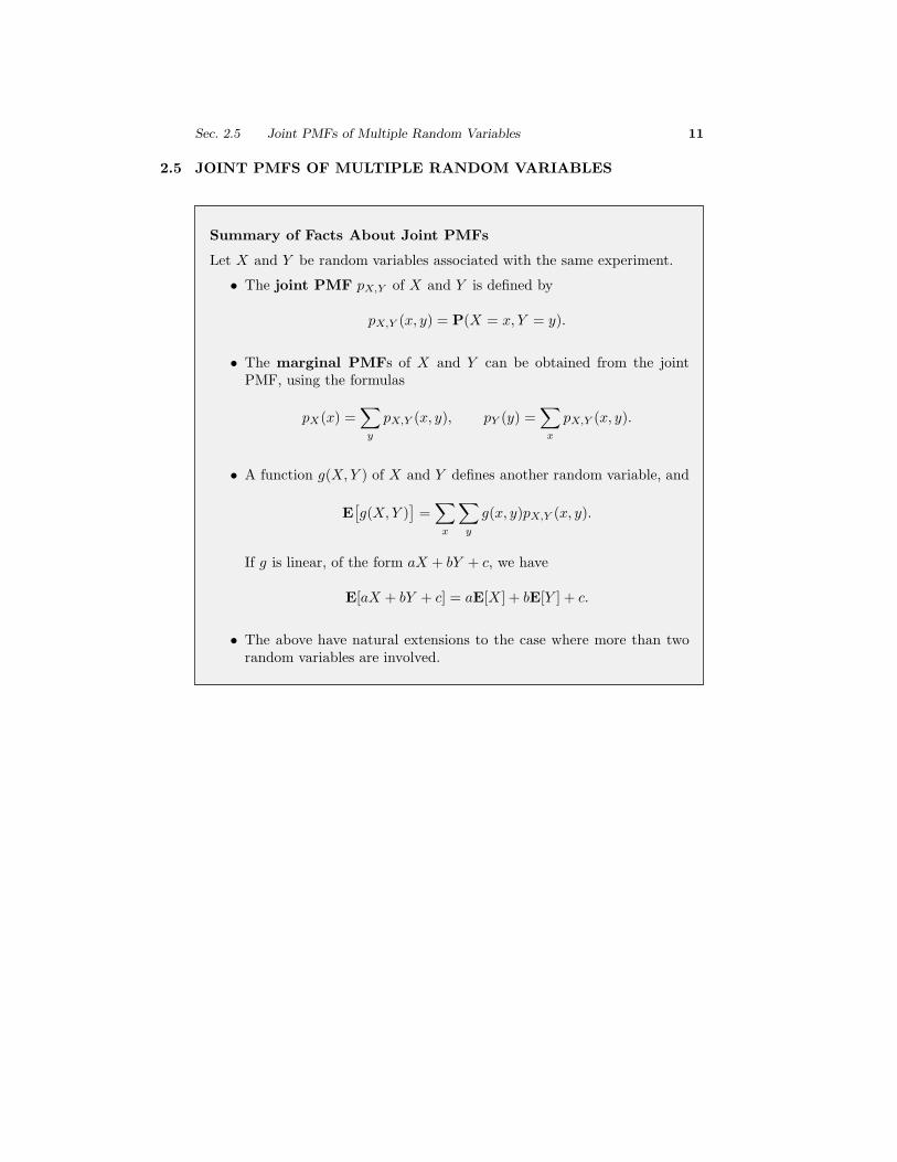
Summary of Facts About Joint PMFs

Let X and Y be random variables associated with the same experiment.

• The joint PMF pX,Y of X and Y is defined by

pX,Y (x, y) = P(X = x, Y = y).

• The marginal PMFs of X and Y can be obtained from the jointPMF, using the formulas

pX(x) =∑

y

pX,Y (x, y), pY (y) =∑

x

pX,Y (x, y).

• A function g(X,Y ) of X and Y defines another random variable, and

E[

g(X,Y )]

=∑

x

∑

y

g(x, y)pX,Y (x, y).

If g is linear, of the form aX + bY + c, we have

E[aX + bY + c] = aE[X ] + bE[Y ] + c.

• The above have natural extensions to the case where more than tworandom variables are involved.


2.6 CONDITIONING

Summary of Facts About Conditional PMFs


• Conditional PMFs are similar to ordinary PMFs, but pertain to auniverse where the conditioning event is known to have occurred.

• The conditional PMF of X given an event A with P(A) > 0, is definedby

pX|A(x) = P(X = x |A)

and satisfies∑

x

pX|A(x) = 1.

• If A1, . . . , An are disjoint events that form a partition of the samplespace, with P(Ai) > 0 for all i, then

pX(x) =

n∑

i=1

P(Ai)pX|Ai(x).

(This is a special case of the total probability theorem.) Furthermore,for any event B, with P(Ai ∩B) > 0 for all i, we have

pX|B(x) =

n∑

i=1

P(Ai |B)pX|Ai∩B(x).

• The conditional PMF of X given Y = y is related to the joint PMFby

pX,Y (x, y) = pY (y)pX|Y (x | y).

• The conditional PMF of X given Y can be used to calculate themarginal PMF of X through the formula

pX(x) =∑

y

pY (y)pX|Y (x | y).

• There are natural extensions of the above involving more than tworandom variables.

Sec. 2.6 Conditioning 13

Summary of Facts About Conditional Expectations


• The conditional expectation of X given an event A with P(A) > 0, isdefined by

E[X |A] =∑

x

xpX|A(x).

For a function g(X), we have

E[

g(X) |A]

=∑

x

g(x)pX|A(x).

• The conditional expectation of X given a value y of Y is defined by

E[X |Y = y] =∑

x

xpX|Y (x | y).

• If A1, . . . , An be disjoint events that form a partition of the samplespace, with P(Ai) > 0 for all i, then

E[X ] =

n∑

i=1

P(Ai)E[X |Ai].

Furthermore, for any event B with P(Ai ∩B) > 0 for all i, we have

E[X |B] =

n∑

i=1

P(Ai |B)E[X |Ai ∩B].

• We haveE[X ] =

∑

y

pY (y)E[X |Y = y].


2.7 INDEPENDENCE

Summary of Facts About Independent Random Variables

Let A be an event, with P(A) > 0, and let X and Y be random variablesassociated with the same experiment.

• X is independent of the event A if

pX|A(x) = pX(x), for all x,

that is, if for all x, the events X = x and A are independent.

• X and Y are independent if for all pairs (x, y), the events X = xand Y = y are independent, or equivalently

pX,Y (x, y) = pX(x)pY (y), for all x, y.

• If X and Y are independent random variables, then

E[XY ] = E[X ]E[Y ].

Furthermore, for any functions g and h, the random variables g(X)and h(Y ) are independent, and we have

E[

g(X)h(Y )]

= E[

g(X)]

E[

h(Y )]

.

• If X and Y are independent, then

var(X + Y ) = var(X) + var(Y ).

Sec. 2.8 Summary and Discussion 15


Summary of Results for Special Random Variables

Discrete Uniform over [a, b]:

pX(k) =

1

b− a+ 1, if k = a, a+ 1, . . . , b,

0, otherwise,

E[X ] =a+ b

2, var(X) =

(b − a)(b− a+ 2)

12.

Bernoulli with Parameter p: (Describes the success or failure in a singletrial.)

pX(k) =

p, if k = 1,1− p, if k = 0,

E[X ] = p, var(X) = p(1− p).

Binomial with Parameters p and n: (Describes the number of successesin n independent Bernoulli trials.)

pX(k) =

(

n

k

)

pk(1− p)n−k, k = 0, 1, . . . , n,

E[X ] = np, var(X) = np(1− p).

Geometric with Parameter p: (Describes the number of trials until thefirst success, in a sequence of independent Bernoulli trials.)

pX(k) = (1− p)k−1p, k = 1, 2, . . . ,

E[X ] =1

p, var(X) =

1− p

p2.

Poisson with Parameter λ: (Approximates the binomial PMF when nis large, p is small, and λ = np.)

pX(k) = e−λλk

k!, k = 0, 1, . . . ,

E[X ] = λ, var(X) = λ.

3

General Random Variables




Contents

3.1. Continuous Random Variables and PDFs . . . . . . . . . p. 1403.2. Cumulative Distribution Functions . . . . . . . . . . . . p. 1483.3. Normal Random Variables . . . . . . . . . . . . . . . . p. 1533.4. Joint PDFs of Multiple Random Variables . . . . . . . . . p. 1583.5. Conditioning . . . . . . . . . . . . . . . . . . . . . p. 1643.6. The Continuous Bayes’ Rule . . . . . . . . . . . . . . . p. 1783.7. Summary and Discussion . . . . . . . . . . . . . . . . p. 182

Problems . . . . . . . . . . . . . . . . . . . . . . . . p. 184

17


3.1 CONTINUOUS RANDOM VARIABLES AND PDFS

Summary of PDF Properties

Let X be a continuous random variable with PDF fX .

• fX(x) ≥ 0 for all x.

•∫ ∞

−∞

fX(x) dx = 1.

• If δ is very small, then P(

[x, x+ δ])

≈ fX(x) · δ.• For any subset B of the real line,

P(X ∈ B) =

∫

B

fX(x) dx.

Expectation of a Continuous Random Variable and its Properties

Let X be a continuous random variable with PDF fX .

• The expectation of X is defined by

E[X ] =

∫ ∞

−∞

xfX(x) dx.

• The expected value rule for a function g(X) has the form

E[

g(X)]

=

∫ ∞

−∞

g(x)fX(x) dx.

• The variance of X is defined by

var(X) = E[(

X −E[X ])2]

=

∫ ∞

−∞

(

x−E[X ])2fX(x) dx.

• We have0 ≤ var(X) = E[X2]−

(

E[X ])2.

• If Y = aX + b, where a and b are given scalars, then

E[Y ] = aE[X ] + b, var(Y ) = a2var(X).

Sec. 3.2 Cumulative Distribution Functions 19

3.2 CUMULATIVE DISTRIBUTION FUNCTIONS

Properties of a CDF

The CDF FX of a random variable X is defined by

FX(x) = P(X ≤ x), for all x,

and has the following properties.

• FX is monotonically nondecreasing:

if x ≤ y, then FX(x) ≤ FX(y).

• FX(x) tends to 0 as x → −∞, and to 1 as x → ∞.

• If X is discrete, then FX(x) is a piecewise constant function of x.

• If X is continuous, then FX(x) is a continuous function of x.

• If X is discrete and takes integer values, the PMF and the CDF canbe obtained from each other by summing or differencing:

FX(k) =

k∑

i=−∞

pX(i),

pX(k) = P(X ≤ k)−P(X ≤ k − 1) = FX(k)− FX(k − 1),

for all integers k.

• If X is continuous, the PDF and the CDF can be obtained from eachother by integration or differentiation:

FX(x) =

∫ x

−∞

fX(t) dt, fX(x) =dFX

dx(x).

(The second equality is valid for those x at which the PDF is contin-uous.)


3.3 NORMAL RANDOM VARIABLES

Normality is Preserved by Linear Transformations

If X is a normal random variable with mean µ and variance σ2, and if a = 0,b are scalars, then the random variable

Y = aX + b

is also normal, with mean and variance

E[Y ] = aµ+ b, var(Y ) = a2σ2.

CDF Calculation for a Normal Random Variable

For a normal random variable X with mean µ and variance σ2, we use atwo-step procedure.

(a) “Standardize” X , i.e., subtract µ and divide by σ to obtain a standardnormal random variable Y .

(b) Read the CDF value from the standard normal table:

P(X ≤ x) = P

(

X − µ

σ≤ x− µ

σ

)

= P

(

Y ≤ x− µ

σ

)

= Φ

(

x− µ

σ

)

.

6

Sec. 3.4 Normal Random Variables 21

.00 .01 .02 .03 .04 .05 .06 .07 .08 .09

0.0 .5000 .5040 .5080 .5120 .5160 .5199 .5239 .5279 .5319 .5359

0.1 .5398 .5438 .5478 .5517 .5557 .5596 .5636 .5675 .5714 .5753

0.2 .5793 .5832 .5871 .5910 .5948 .5987 .6026 .6064 .6103 .6141

0.3 .6179 .6217 .6255 .6293 .6331 .6368 .6406 .6443 .6480 .6517

0.4 .6554 .6591 .6628 .6664 .6700 .6736 .6772 .6808 .6844 .6879

0.5 .6915 .6950 .6985 .7019 .7054 .7088 .7123 .7157 .7190 .7224

0.6 .7257 .7291 .7324 .7357 .7389 .7422 .7454 .7486 .7517 .7549

0.7 .7580 .7611 .7642 .7673 .7704 .7734 .7764 .7794 .7823 .7852

0.8 .7881 .7910 .7939 .7967 .7995 .8023 .8051 .8078 .8106 .8133

0.9 .8159 .8186 .8212 .8238 .8264 .8289 .8315 .8340 .8365 .8389

1.0 .8413 .8438 .8461 .8485 .8508 .8531 .8554 .8577 .8599 .8621

1.1 .8643 .8665 .8686 .8708 .8729 .8749 .8770 .8790 .8810 .8830

1.2 .8849 .8869 .8888 .8907 .8925 .8944 .8962 .8980 .8997 .9015

1.3 .9032 .9049 .9066 .9082 .9099 .9115 .9131 .9147 .9162 .9177

1.4 .9192 .9207 .9222 .9236 .9251 .9265 .9279 .9292 .9306 .9319

1.5 .9332 .9345 .9357 .9370 .9382 .9394 .9406 .9418 .9429 .9441

1.6 .9452 .9463 .9474 .9484 .9495 .9505 .9515 .9525 .9535 .9545

1.7 .9554 .9564 .9573 .9582 .9591 .9599 .9608 .9616 .9625 .9633

1.8 .9641 .9649 .9656 .9664 .9671 .9678 .9686 .9693 .9699 .9706

1.9 .9713 .9719 .9726 .9732 .9738 .9744 .9750 .9756 .9761 .9767

2.0 .9772 .9778 .9783 .9788 .9793 .9798 .9803 .9808 .9812 .9817

2.1 .9821 .9826 .9830 .9834 .9838 .9842 .9846 .9850 .9854 .9857

2.2 .9861 .9864 .9868 .9871 .9875 .9878 .9881 .9884 .9887 .9890

2.3 .9893 .9896 .9898 .9901 .9904 .9906 .9909 .9911 .9913 .9916

2.4 .9918 .9920 .9922 .9925 .9927 .9929 .9931 .9932 .9934 .9936

2.5 .9938 .9940 .9941 .9943 .9945 .9946 .9948 .9949 .9951 .9952

2.6 .9953 .9955 .9956 .9957 .9959 .9960 .9961 .9962 .9963 .9964

2.7 .9965 .9966 .9967 .9968 .9969 .9970 .9971 .9972 .9973 .9974

2.8 .9974 .9975 .9976 .9977 .9977 .9978 .9979 .9979 .9980 .9981

2.9 .9981 .9982 .9982 .9983 .9984 .9984 .9985 .9985 .9986 .9986

3.0 .9987 .9987 .9987 .9988 .9988 .9989 .9989 .9989 .9990 .9990

3.1 .9990 .9991 .9991 .9991 .9992 .9992 .9992 .9992 .9993 .9993

3.2 .9993 .9993 .9994 .9994 .9994 .9994 .9994 .9995 .9995 .9995

3.3 .9995 .9995 .9995 .9996 .9996 .9996 .9996 .9996 .9996 .9997

3.4 .9997 .9997 .9997 .9997 .9997 .9997 .9997 .9997 .9997 .9998

The standard normal table. The entries in this table provide the numerical values

of Φ(y) = P(Y ≤ y), where Y is a standard normal random variable, for y between 0

and 3.49. For example, to find Φ(1.71), we look at the row corresponding to 1.7 and

the column corresponding to 0.01, so that Φ(1.71) = .9564. When y is negative, the

value of Φ(y) can be found using the formula Φ(y) = 1−Φ(−y).


3.4 JOINT PDFS OF MULTIPLE RANDOM VARIABLES

Summary of Facts about Joint PDFs

Let X and Y be jointly continuous random variables with joint PDF fX,Y .

• The joint PDF is used to calculate probabilities:

P(

(X,Y ) ∈ B)

=

∫ ∫

(x,y)∈B

fX,Y (x, y) dx dy.

• The marginal PDFs of X and Y can be obtained from the joint PDF,using the formulas

fX(x) =

∫ ∞

−∞

fX,Y (x, y) dy, fY (y) =

∫ ∞

−∞

fX,Y (x, y) dx.

• The joint CDF is defined by FX,Y (x, y) = P(X ≤ x, Y ≤ y), anddetermines the joint PDF through the formula

fX,Y (x, y) =∂2FX,Y

∂x∂y(x, y),

for every (x, y) at which the joint PDF is continuous.

• A function g(X,Y ) of X and Y defines a new random variable, and

E[

g(X,Y )]

=

∫ ∞

−∞

∫ ∞

−∞

g(x, y)fX,Y (x, y) dx dy.

If g is linear, of the form aX + bY + c, we have

E[aX + bY + c] = aE[X ] + bE[Y ] + c.

• The above have natural extensions to the case where more than tworandom variables are involved.


3.5 CONDITIONING

Conditional PDF Given an Event

• The conditional PDF fX|A of a continuous random variable X , givenan event A with P(A) > 0, satisfies

P(X ∈ B |A) =∫

B

fX|A(x) dx.

• If A is a subset of the real line with P(X ∈ A) > 0, then

fX|X∈A(x) =

fX(x)

P(X ∈ A), if x ∈ A,

0, otherwise.

• Let A1, A2, . . . , An be disjoint events that form a partition of the sam-ple space, and assume that P(Ai) > 0 for all i. Then,

fX(x) =

n∑

i=1

P(Ai)fX|Ai(x)

(a version of the total probability theorem).

Conditional PDF Given a Random Variable

Let X and Y be jointly continuous random variables with joint PDF fX,Y .

• The joint, marginal, and conditional PDFs are related to each otherby the formulas

fX,Y (x, y) = fY (y)fX|Y (x | y),

fX(x) =

∫ ∞

−∞

fY (y)fX|Y (x | y) dy.

The conditional PDF fX|Y (x | y) is defined only for those y for whichfY (y) > 0.

• We have

P(X ∈ A |Y = y) =

∫

A

fX|Y (x | y) dx.


Summary of Facts About Conditional Expectations

Let X snd Y be jointly continuous random variables, and let A be an eventwith P(A) > 0.

• Definitions: The conditional expectation of X given the event A isdefined by

E[X |A] =∫ ∞

−∞

xfX|A(x) dx.

The conditional expectation of X given that Y = y is defined by

E[X |Y = y] =

∫ ∞

−∞

xfX|Y (x | y) dx.

• The expected value rule: For a function g(X), we have

E[

g(X) |A]

=

∫ ∞

−∞

g(x)fX|A(x) dx,

and

E[

g(X) |Y = y]

=

∫ ∞

−∞

g(x)fX|Y (x | y) dx.

• Total expectation theorem: Let A1, A2, . . . , An be disjoint eventsthat form a partition of the sample space, and assume that P(Ai) > 0for all i. Then,

E[X ] =

n∑

i=1

P(Ai)E[X |Ai].

Similarly,

E[X ] =

∫ ∞

−∞

E[X |Y = y]fY (y) dy.

• There are natural analogs for the case of functions of several randomvariables. For example,

E[

g(X,Y ) |Y = y]

=

∫

g(x, y)fX|Y (x | y) dx,

and

E[

g(X,Y )]

=

∫

E[

g(X,Y ) |Y = y]fY (y) dy.


Independence of Continuous Random Variables

Let X and Y be jointly continuous random variables.

• X and Y are independent if

fX,Y (x, y) = fX(x)fY (y), for all x, y.


E[XY ] = E[X ]E[Y ].

Furthermore, for any functions g and h, the random variables g(X)and h(Y ) are independent, and we have

E[

g(X)h(Y )]

= E[

g(X)]

E[

h(Y )]

.


var(X + Y ) = var(X) + var(Y ).


3.6 BAYES’ RULE AND APPLICATIONS IN INFERENCE

Bayes’ Rule Relations for Random Variables

Let X and Y be two random variables.

• If X and Y are discrete, we have for all x, y with pX(x) = 0, pY (y) = 0,

pX(x)pY |X(y |x) = pY (y)pX|Y (x | y),

and the terms on the two sides in this relation are both equal to

pX,Y (x, y).

• IfX is discrete and Y is continuous, we have for all x, y with pX(x) = 0,fY (y) = 0,

pX(x)fY |X(y |x) = fY (y)pX|Y (x | y),


limδ→0

P(X = x, y ≤ Y ≤ y + δ)

δ.

• If X and Y are continuous, we have for all x, y with fX(x) = 0,fY (y) = 0,

fX(x)fY |X(y |x) = fY (y)fX|Y (x | y),


limδ→0

P(x ≤ X ≤ x+ δ, y ≤ Y ≤ y + δ)

δ2.

6 6

66

66



Summary of Results for Special Random Variables

Continuous Uniform Over [a, b]:

fX(x) =

1

b− a, if a ≤ x ≤ b,

0, otherwise,

E[X ] =a+ b

2, var(X) =

(b− a)2

12.

Exponential with Parameter λ:

fX(x) =

λe−λx, if x ≥ 0,0, otherwise,

FX(x) =

1− e−λx, if x ≥ 0,0, otherwise,

E[X ] =1

λ, var(X) =

1

λ2.

Normal with Parameters µ and σ2 > 0:

fX(x) =1√2π σ

e−(x−µ)2/2σ2

,

E[X ] = µ, var(X) = σ2.

4

Further Topics

on Random Variables




Contents

4.1. Derived Distributions . . . . . . . . . . . . . . . . . . p. 2024.2. Covariance and Correlation . . . . . . . . . . . . . . . p. 2174.3. Conditional Expectation and Variance Revisited . . . . . . p. 2224.4. Transforms . . . . . . . . . . . . . . . . . . . . . . p. 2294.5. Sum of a Random Number of Independent Random Variables p. 2404.6. Summary and Discussion . . . . . . . . . . . . . . . . p. 244

Problems . . . . . . . . . . . . . . . . . . . . . . . . p. 246

29


4.1 DERIVED DISTRIBUTIONS

Calculation of the PDF of a Function Y = g(X) of a ContinuousRandom Variable X

1. Calculate the CDF FY of Y using the formula

FY (y) = P(

g(X) ≤ y)

=

∫

x | g(x)≤y

fX(x) dx.

2. Differentiate to obtain the PDF of Y :

fY (y) =dFY

dy(y).

The PDF of a Linear Function of a Random Variable

Let X be a continuous random variable with PDF fX , and let

Y = aX + b,

where a and b are scalars, with a = 0. Then,

fY (y) =1

|a|fX(

y − b

a

)

.

6

Sec. 4.2 Covariance and Correlation 31

PDF Formula for a Strictly Monotonic Function of a ContinuousRandom Variable

Suppose that g is strictly monotonic and that for some function h and all xin the range of X we have

y = g(x) if and only if x = h(y).

Assume that h is differentiable. Then, the PDF of Y in the region wherefY (y) > 0 is given by

fY (y) = fX(

h(y))

∣

∣

∣

∣

dh

dy(y)

∣

∣

∣

∣

.

4.2 COVARIANCE AND CORRELATION

Covariance and Correlation

• The covariance of X and Y is given by

cov(X,Y ) = E[

(

X −E[X ])(

Y −E[Y ])

]

= E[XY ]−E[X ]E[Y ].

• If cov(X,Y ) = 0, we say that X and Y are uncorrelated.

• If X and Y are independent, they are uncorrelated. The converse isnot always true.

• We have

var(X + Y ) = var(X) + var(Y ) + 2cov(X,Y ).

• The correlation coefficient ρ(X,Y ) of two random variables X andY with positive variances is defined by

ρ(X,Y ) =cov(X,Y )

√

var(X)var(Y ),

and satisfies−1 ≤ ρ(X,Y ) ≤ 1.


4.3 CONDITIONAL EXPECTATION AND VARIANCE REVISITED

Law of Iterated Expectations: E[

E[X |Y ]]

= E[X ].

Law of Total Variance: var(X) = E[

var(X |Y )]

+ var(

E[X |Y ])

.

Properties of the Conditional Expectation and Variance

• E[X |Y = y] is a number whose value depends on y.

• E[X |Y ] is a function of the random variable Y , hence a random vari-able. Its value is E[X |Y = y] whenever the value of Y is y.

• E[

E[X |Y ]]

= E[X ] (law of iterated expectations).

• E[X |Y = y] may be viewed as an estimate of X given Y = y. Thecorresponding error E[X |Y ]−X is a zero mean random variable thatis uncorrelated with E[X |Y ].

• var(X |Y ) is a random variable whose value is var(X |Y = y) wheneverthe value of Y is y.

• var(X) = E[

var(X |Y )]

+ var(

E[X |Y ])

(law of total variance).

Sec. 4.4 Transforms 33

4.4 TRANSFORMS

Summary of Transforms and their Properties

• The transform associated with a random variable X is given by

MX(s) = E[esX ] =

∑

x

esxpX(x), X discrete,

∫ ∞

−∞

esxfX(x) dx, X continuous.

• The distribution of a random variable is completely determined by thecorresponding transform.

• Moment generating properties:

MX(0) = 1,d

dsMX(s)

∣

∣

∣

∣

s=0

= E[X ],dn

dsnMX(s)

∣

∣

∣

∣

s=0

= E[Xn].

• If Y = aX + b, then MY (s) = esbMX(as).

• If X and Y are independent, then MX+Y (s) = MX(s)MY (s).


Transforms for Common Discrete Random Variables

Bernoulli(p) (k = 0, 1)

pX(k) =

p, if k = 1,1− p, if k = 0,

MX(s) = 1− p+ pes.

Binomial(n, p) (k = 0, 1, . . . , n)

pX(k) =

(

n

k

)

pk(1 − p)n−k, MX(s) = (1− p+ pes)n.

Geometric(p) (k = 1, 2, . . .)

pX(k) = p(1− p)k−1, MX(s) =pes

1− (1− p)es.

Poisson(λ) (k = 0, 1, . . .)

pX(k) =e−λλk

k!, MX(s) = eλ(e

s−1).

Uniform(a, b) (k = a, a+ 1, . . . , b)

pX(k) =1

b− a+ 1, MX(s) =

esa(

es(b−a+1) − 1)

(b − a+ 1)(es − 1).

Transforms for Common Continuous Random Variables

Uniform(a, b) (a ≤ x ≤ b)

fX(x) =1

b− a, MX(s) =

esb − esa

s(b− a).

Exponential(λ) (x ≥ 0)

fX(x) = λe−λx, MX(s) =λ

λ− s, (s < λ).

Normal(µ, σ2) (−∞ < x < ∞)

fX(x) =1√2π σ

e−(x−µ)2/2σ2

, MX(s) = e(σ2s2/2)+µs.


4.5 SUM OF A RANDOMNUMBEROF INDEPENDENTRANDOMVARIABLES

Properties of the Sum of a Random Number of Independent Ran-dom Variables

Let X1, X2, . . . be identically distributed random variables with mean E[X ]and variance var(X). Let N be a random variable that takes nonnegative in-teger values. We assume that all of these random variables are independent,and we consider the sum

Y = X1 + · · ·+XN .

Then:

• E[Y ] = E[N ]E[X ].

• var(Y ) = E[N ] var(X) +(

E[X ])2var(N).

• We haveMY (s) = MN

(

logMX(s))

.

Equivalently, the transform MY (s) is found by starting with the trans-form MN(s) and replacing each occurrence of es with MX(s).


5

Limit Theorems




Contents

5.1. Markov and Chebyshev Inequalities . . . . . . . . . . . . p. 2655.2. The Weak Law of Large Numbers . . . . . . . . . . . . . p. 2695.3. Convergence in Probability . . . . . . . . . . . . . . . . p. 2715.4. The Central Limit Theorem . . . . . . . . . . . . . . . p. 2735.5. The Strong Law of Large Numbers . . . . . . . . . . . . p. 2805.6. Summary and Discussion . . . . . . . . . . . . . . . . p. 282

Problems . . . . . . . . . . . . . . . . . . . . . . . . p. 284

37


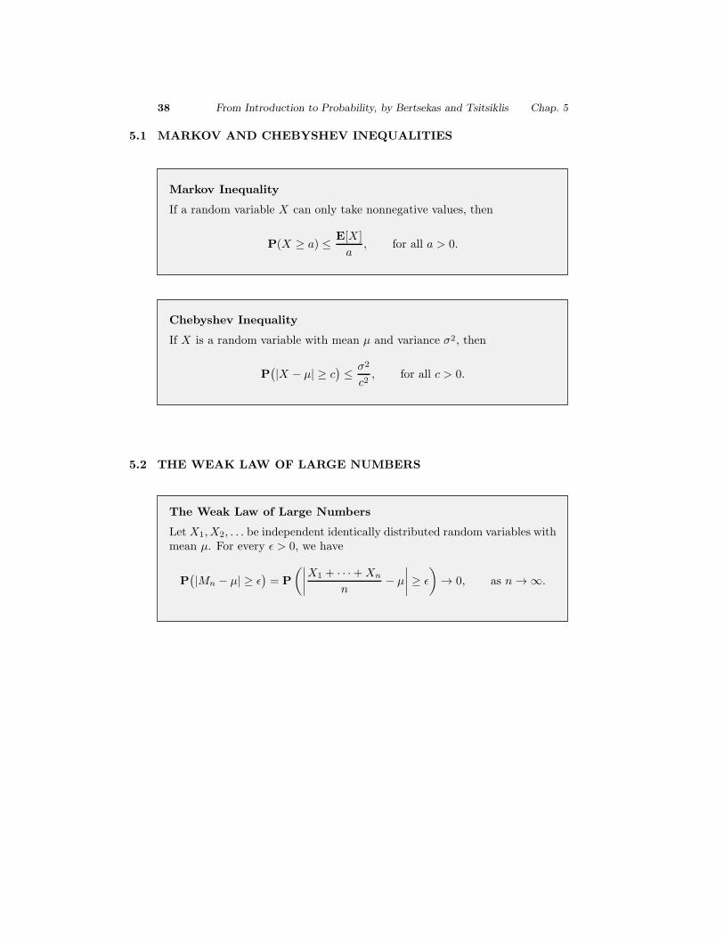
5.1 MARKOV AND CHEBYSHEV INEQUALITIES

Markov Inequality

If a random variable X can only take nonnegative values, then

P(X ≥ a) ≤ E[X ]

a, for all a > 0.

Chebyshev Inequality

If X is a random variable with mean µ and variance σ2, then

P(

|X − µ| ≥ c)

≤ σ2

c2, for all c > 0.

5.2 THE WEAK LAW OF LARGE NUMBERS

The Weak Law of Large Numbers

Let X1, X2, . . . be independent identically distributed random variables withmean µ. For every ǫ > 0, we have

X1 + +XnP(

|Mn − µ·| ≥ ǫ

)

= P

(∣

∣ · ·∣ µ ǫ 0, as n .∣ n

−∣

∣

∣ ≥)

→ → ∞∣

Sec. 5.3 Convergence in Probability 39

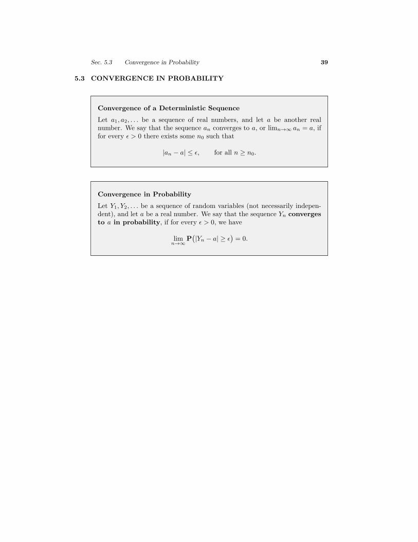
5.3 CONVERGENCE IN PROBABILITY

Convergence of a Deterministic Sequence

Let a1, a2, . . . be a sequence of real numbers, and let a be another realnumber. We say that the sequence an converges to a, or limn→∞ an = a, iffor every ǫ > 0 there exists some n0 such that

|an − a| ≤ ǫ, for all n ≥ n0.

Convergence in Probability

Let Y1, Y2, . . . be a sequence of random variables (not necessarily indepen-dent), and let a be a real number. We say that the sequence Yn convergesto a in probability, if for every ǫ > 0, we have

limn→∞

P(

|Yn − a| ≥ ǫ)

= 0.


5.4 THE CENTRAL LIMIT THEOREM

The Central Limit Theorem

Let X1, X2, . . . be a sequence of independent identically distributed randomvariables with common mean µ and variance σ2, and define

Zn =X1 + · · ·+Xn − nµ

σ√n

.

Then, the CDF of Zn converges to the standard normal CDF

Φ(z) =1√2π

∫ z

−∞

e−x2/2 dx,

in the sense that

limn→∞

P(Zn ≤ z) = Φ(z), for every z.

Normal Approximation Based on the Central Limit Theorem

Let Sn = X1 + · · · + Xn, where the Xi are independent identically dis-tributed random variables with mean µ and variance σ2. If n is large, theprobability P(Sn ≤ c) can be approximated by treating Sn as if it werenormal, according to the following procedure.

1. Calculate the mean nµ and the variance nσ2 of Sn.

2. Calculate the normalized value z = (c− nµ)/σ√n.

3. Use the approximation

P(Sn ≤ c) ≈ Φ(z),

where Φ(z) is available from standard normal CDF tables.


De Moivre-Laplace Approximation to the Binomial

If Sn is a binomial random variable with parameters n and p, n is large, andk, l are nonnegative integers, then

P(k ≤ Sn ≤ l) ≈ Φ

(

l + 12 − np

√

np(1− p)

)

− Φ

(

k − 12 − np

√

np(1− p)

)

.

5.5 THE STRONG LAW OF LARGE NUMBERS

The Strong Law of Large Numbers

Let X1, X2, . . . be a sequence of independent identically distributed randomvariables with mean µ. Then, the sequence of sample means Mn = (X1 +· · ·+Xn)/n converges to µ, with probability 1, in the sense that

P

(

limn→∞

X1 + · · ·+Xn

n= µ

)

= 1.

Convergence with Probability 1

Let Y1, Y2, . . . be a sequence of random variables (not necessarily indepen-dent). Let c be a real number. We say that Yn converges to c with prob-ability 1 (or almost surely) if

P(

limn→∞

Yn = c)

= 1.


6

The Bernoulli and Poisson

Processes




Contents

6.1. The Bernoulli Process . . . . . . . . . . . . . . . . . . p. 2976.2. The Poisson Process . . . . . . . . . . . . . . . . . . p. 3096.3. Summary and Discussion . . . . . . . . . . . . . . . . p. 324

Problems . . . . . . . . . . . . . . . . . . . . . . . . p. 326

43


6.1 THE BERNOULLI PROCESS

Some Random Variables Associated with the Bernoulli Processand their Properties

• The binomial with parameters p and n. This is the number S ofsuccesses in n independent trials. Its PMF, mean, and variance are

pS(k) =

(

n

k

)

pk(1− p)n−k, k = 0, 1, . . . , n,

E[S] = np, var(S) = np(1− p).

• The geometric with parameter p. This is the number T of trialsup to (and including) the first success. Its PMF, mean, and varianceare

pT (t) = (1− p)t−1p, t = 1, 2, . . . ,

E[T ] =1

p, var(T ) =

1− p

p2.

Independence Properties of the Bernoulli Process

• For any given time n, the sequence of random variablesXn+1, Xn+2, . . .(the future of the process) is also a Bernoulli process, and is indepen-dent from X1, . . . , Xn (the past of the process).

• Let n be a given time and let T be the time of the first success aftertime n. Then, T − n has a geometric distribution with parameter p,and is independent of the random variables X1, . . . , Xn.

Alternative Description of the Bernoulli Process

1. Start with a sequence of independent geometric random variables T1,T2, . . ., with common parameter p, and let these stand for the interar-rival times.

2. Record a success (or arrival) at times T1, T1 + T2, T1 + T2 + T3, etc.

Sec. 6.1 The Bernoulli Process 45

Properties of the kth Arrival Time

• The kth arrival time is equal to the sum of the first k interarrival times

Yk = T1 + T2 + · · ·+ Tk,

and the latter are independent geometric random variables with com-mon parameter p.

• The mean and variance of Yk are given by

E[Yk] = E[T1] + · · ·+E[Tk] =k

p,

var(Yk) = var(T1) + · · ·+ var(Tk) =k(1− p)

p2.

• The PMF of Yk is given by

pYk(t) =

(

t− 1

k − 1

)

pk(1− p)t−k, t = k, k + 1, . . . ,

and is known as the Pascal PMF of order k.


Poisson Approximation to the Binomial

• A Poisson random variable Z with parameter λ takes nonnegativeinteger values and is described by the PMF

pZ(k) = e−λλk

k!, k = 0, 1, 2, . . . .

Its mean and variance are given by

E[Z] = λ, var(Z) = λ.

• For any fixed nonnegative integer k, the binomial probability

pS(k) =n!

(n− k)! k!· pk(1− p)n−k

converges to pZ(k), when we take the limit as n → ∞ and p = λ/n,while keeping λ constant.

• In general, the Poisson PMF is a good approximation to the binomialas long as λ = np, n is very large, and p is very small.

Sec. 6.2 The Poisson Process 47

6.2 THE POISSON PROCESS

Definition of the Poisson Process

An arrival process is called a Poisson process with rate λ if it has the fol-lowing properties:

(a) (Time-homogeneity) The probability P (k, τ) of k arrivals is thesame for all intervals of the same length τ .

(b) (Independence) The number of arrivals during a particular intervalis independent of the history of arrivals outside this interval.

(c) (Small interval probabilities) The probabilities P (k, τ) satisfy

P (0, τ) = 1− λτ + o(τ),

P (1, τ) = λτ + o1(τ),

P (k, τ) = ok(τ), for k = 2, 3, . . .

Here, o(τ) and ok(τ) are functions of τ that satisfy

limτ→0

o(τ)

τ= 0, lim

τ→0

ok(τ)

τ= 0.

Random Variables Associated with the Poisson Process and theirProperties

• The Poisson with parameter λτ . This is the number Nτ of arrivalsin a Poisson process with rate λ, over an interval of length τ . Its PMF,mean, and variance are

pNτ(k) = P (k, τ) = e−λτ

(λτ)k

k!, k = 0, 1, . . . ,

E[Nτ ] = λτ, var(Nτ ) = λτ.

• The exponential with parameter λ. This is the time T until thefirst arrival. Its PDF, mean, and variance are

fT (t) = λe−λt, t ≥ 0, E[T ] =1

λ, var(T ) =

1

λ2.


Independence Properties of the Poisson Process

• For any given time t > 0, the history of the process after time t is alsoa Poisson process, and is independent from the history of the processuntil time t.

• Let t be a given time and let T be the time of the first arrival aftertime t. Then, T − t has an exponential distribution with parameter λ,and is independent of the history of the process until time t.

Alternative Description of the Poisson Process

1. Start with a sequence of independent exponential random variablesT1, T2,. . ., with common parameter λ, and let these represent the in-terarrival times.

2. Record an arrival at times T1, T1 + T2, T1 + T2 + T3, etc.

Properties of the kth Arrival Time

• The kth arrival time is equal to the sum of the first k interarrival times

Yk = T1 + T2 + · · ·+ Tk,

and the latter are independent exponential random variables with com-mon parameter λ.

• The mean and variance of Yk are given by

E[Yk] = E[T1] + · · ·+E[Tk] =k

λ,

var(Yk) = var(T1) + · · ·+ var(Tk) =k

λ2.

• The PDF of Yk is given by

fYk(y) =

λkyk−1e−λy

(k − 1)!, y ≥ 0,

and is known as the Erlang PDF of order k.


Properties of Sums of a Random Number of Random Variables

Let N,X1, X2, . . . be independent random variables, where N takes nonneg-ative integer values. Let Y = X1 + · · · +XN for positive values of N , andlet Y = 0 when N = 0.

• If Xi is Bernoulli with parameter p, and N is binomial with parametersm and q, then Y is binomial with parameters m and pq.

• If Xi is Bernoulli with parameter p, and N is Poisson with parameterλ, then Y is Poisson with parameter λp.

• If Xi is geometric with parameter p, and N is geometric with param-eter q, then Y is geometric with parameter pq.

• If Xi is exponential with parameter λ, and N is geometric with pa-rameter q, then Y is exponential with parameter λq.


7

Markov Chains




Contents

7.1. Discrete-Time Markov Chains . . . . . . . . . . . . . . p. 3407.2. Classification of States . . . . . . . . . . . . . . . . . . p. 3467.3. Steady-State Behavior . . . . . . . . . . . . . . . . . . p. 3527.4. Absorption Probabilities and Expected Time to Absorption . p. 3627.5. Continuous-Time Markov Chains . . . . . . . . . . . . . p. 3697.6. Summary and Discussion . . . . . . . . . . . . . . . . p. 378

Problems . . . . . . . . . . . . . . . . . . . . . . . . p. 380

51


7.1 DISCRETE-TIME MARKOV CHAINS

Specification of Markov Models

• A Markov chain model is specified by identifying:

(a) the set of states § = 1, . . . ,m,(b) the set of possible transitions, namely, those pairs (i, j) for which

pij > 0, and,

(c) the numerical values of those pij that are positive.

• The Markov chain specified by this model is a sequence of randomvariables X0, X1, X2, . . ., that take values in §, and which satisfy

P(Xn+1 = j |Xn = i,Xn−1 = in−1, . . . , X0 = i0) = pij ,

for all times n, all states i, j ∈ §, and all possible sequences i0, . . . , in−1

of earlier states.

Chapman-Kolmogorov Equation for the n-Step TransitionProbabilities

The n-step transition probabilities can be generated by the recursive formula

rij(n) =m∑

k=1

rik(n− 1)pkj , for n > 1, and all i, j,

starting withrij(1) = pij .

Sec. 7.2 Classification of States 53

7.2 CLASSIFICATION OF STATES

Markov Chain Decomposition

• A Markov chain can be decomposed into one or more recurrent classes,plus possibly some transient states.

• A recurrent state is accessible from all states in its class, but is notaccessible from recurrent states in other classes.

• A transient state is not accessible from any recurrent state.

• At least one, possibly more, recurrent states are accessible from a giventransient state.

Periodicity

Consider a recurrent class R.

• The class is called periodic if its states can be grouped in d > 1disjoint subsets S1, . . . , Sd, so that all transitions from Sk lead to Sk+1

(or to S1 if k = d).

• The class is aperiodic (not periodic) if and only if there exists a timen such that rij(n) > 0, for all i, j ∈ R.


7.3 STEADY-STATE BEHAVIOR

Steady-State Convergence Theorem

Consider a Markov chain with a single recurrent class, which is aperiodic.Then, the states j are associated with steady-state probabilities πj thathave the following properties.

(a) For each j, we have

limn→∞

rij(n) = πj , for all i.

(b) The πj are the unique solution to the system of equations below:

πj =m∑

k=1

πkpkj , j = 1, . . . ,m,

1 =

m∑

k=1

πk.

(c) We haveπj = 0, for all transient states j,

πj > 0, for all recurrent states j.

Steady-State Probabilities as Expected State Frequencies

For a Markov chain with a single class which is aperiodic, the steady-stateprobabilities πj satisfy

πj = limn→∞

vij(n)

n,

where vij(n) is the expected value of the number of visits to state j withinthe first n transitions, starting from state i.

Sec. 7.4 Absorption Probabilities and Expected Time to Absorption 55

Expected Frequency of a Particular Transition

Consider n transitions of a Markov chain with a single class which is aperi-odic, starting from a given initial state. Let qjk(n) be the expected numberof such transitions that take the state from j to k. Then, regardless of theinitial state, we have

limn→∞

qjk(n)

n= πjpjk.

7.4 ABSORPTION PROBABILITIES AND EXPECTED TIMETO ABSORPTION

Absorption Probability Equations

Consider a Markov chain where each state is either transient or absorb-ing, and fix a particular absorbing state s. Then, the probabilities ai ofeventually reaching state s, starting from i, are the unique solution to theequations

as = 1,

ai = 0, for all absorbing i = s,

ai =

m∑

j=1

pijaj , for all transient i.

6


Equations for the Expected Times to Absorption

Consider a Markov chain where all states are transient, except for a singleabsorbing state. The expected times to absorption, µ1, . . . , µm, are theunique solution to the equations

µi = 0, if i is the absorbing state,

µi = 1 +

m∑

j=1

pijµj , if i is transient.

Equations for Mean First Passage and Recurrence Times

Consider a Markov chain with a single recurrent class, and let s be a par-ticular recurrent state.

• The mean first passage times µi to reach state s starting from i, arethe unique solution to the system of equations

µs = 0, µi = 1 +

m∑

j=1

pijµj , for all i = s.

• The mean recurrence time µ∗s of state s is given by

µ∗s = 1 +

m∑

j=1

psjµj .

6

Sec. 7.5 Continuous-Time Markov Chains 57

7.5 CONTINUOUS-TIME MARKOV CHAINS

Continuous-Time Markov Chain Assumptions

• If the current state is i, the time until the next transition is exponen-tially distributed with a given parameter νi, independent of the pasthistory of the process and of the next state.

• If the current state is i, the next state will be j with a given probabilitypij , independent of the past history of the process and of the time untilthe next transition.


Alternative Description of a Continuous-Time Markov Chain

Given the current state i of a continuous-time Markov chain, and for anyj = i, the state δ time units later is equal to j with probability

qijδ + o(δ),

independent of the past history of the process.

Steady-State Convergence Theorem

Consider a continuous-time Markov chain with a single recurrent class.Then, the states j are associated with steady-state probabilities πj thathave the following properties.

(a) For each j, we have

limt→∞

P(

X(t) = j |X(0) = i)

= πj , for all i.

(b) The πj are the unique solution to the system of equations below:

πj

∑

k=j

qjk =∑

k=j

πkqkj , j = 1, . . . ,m,

1 =m∑

k=1

πk.

(c) We haveπj = 0, for all transient states j,

πj > 0, for all recurrent states j.

6

6 6


8

Bayesian Statistical Inference




Contents

8.1. Bayesian Inference and the Posterior Distribution . . . . . p. 4128.2. Point Estimation, Hypothesis Testing, and the MAP Rule . . p. 4208.3. Bayesian Least Mean Squares Estimation . . . . . . . . . p. 4308.4. Bayesian Linear Least Mean Squares Estimation . . . . . . p. 4378.5. Summary and Discussion . . . . . . . . . . . . . . . . p. 444

Problems . . . . . . . . . . . . . . . . . . . . . . . . p. 446

59


Major Terms, Problems, and Methods in this Chapter

• Bayesian statistics treats unknown parameters as random variableswith known prior distributions.

• In parameter estimation, we want to generate estimates that areclose to the true values of the parameters in some probabilistic sense.

• In hypothesis testing, the unknown parameter takes one of a finitenumber of values, corresponding to competing hypotheses; we want tochoose one of the hypotheses, aiming to achieve a small probability oferror.

• Principal Bayesian inference methods:

(a) Maximum a posteriori probability (MAP) rule: Out of thepossible parameter values/hypotheses, select one with maximumconditional/posterior probability given the data (Section 8.2).

(b) Least mean squares (LMS) estimation: Select an estimator/fun-ction of the data that minimizes the mean squared error betweenthe parameter and its estimate (Section 8.3).

(c) Linear least mean squares estimation: Select an estimatorwhich is a linear function of the data and minimizes the meansquared error between the parameter and its estimate (Section8.4). This may result in higher mean squared error, but requiressimple calculations, based only on the means, variances, and co-variances of the random variables involved.

8.1 BAYESIAN INFERENCEAND THE POSTERIORDISTRIBUTION

Summary of Bayesian Inference

• We start with a prior distribution pΘ or fΘ for the unknown randomvariable Θ.

• We have a model pX|Θ or fX|Θ of the observation vector X .

• After observing the value x of X , we form the posterior distributionof Θ, using the appropriate version of Bayes’ rule.

Sec. 8.1 Bayesian Inference and the Posterior Distribution 61

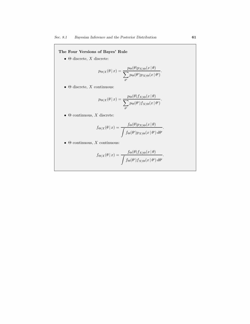
The Four Versions of Bayes’ Rule

• Θ discrete, X discrete:

pΘ|X(θ |x) = pΘ(θ)pX|Θ(x | θ)∑

θ′

pΘ(θ′)pX|Θ(x | θ′).

• Θ discrete, X continuous:

pΘ|X(θ |x) = pΘ(θ)fX|Θ(x | θ)∑

θ′

pΘ(θ′)fX|Θ(x | θ′).

• Θ continuous, X discrete:

fΘ|X(θ |x) = fΘ(θ)pX|Θ(x | θ)∫

fΘ(θ′)pX|Θ(x | θ′) dθ′.

• Θ continuous, X continuous:

fΘ|X(θ |x) = fΘ(θ)fX|Θ(x | θ)∫

fΘ(θ′)fX|Θ(x | θ′) dθ′.


8.2 POINT ESTIMATION, HYPOTHESIS TESTING, AND THEMAP RULE

The Maximum a Posteriori Probability (MAP) Rule

• Given the observation value x, the MAP rule selects a value θ thatmaximizes over θ the posterior distribution pΘ|X(θ |x) (if Θ is discrete)or fΘ|X(θ |x) (if Θ is continuous).

• Equivalently, it selects θ that maximizes over θ:

pΘ(θ)pX|Θ(x | θ) (if Θ and X are discrete),

pΘ(θ)fX|Θ(x | θ) (if Θ is discrete and X is continuous),

fΘ(θ)pX|Θ(x | θ) (if Θ is continuous and X is discrete),

fΘ(θ)fX|Θ(x | θ) (if Θ and X are continuous).

• If Θ takes only a finite number of values, the MAP rule minimizes (overall decision rules) the probability of selecting an incorrect hypothesis.This is true for both the unconditional probability of error and theconditional one, given any observation value x.

Sec. 8.3 Bayesian Least Mean Squares Estimation 63

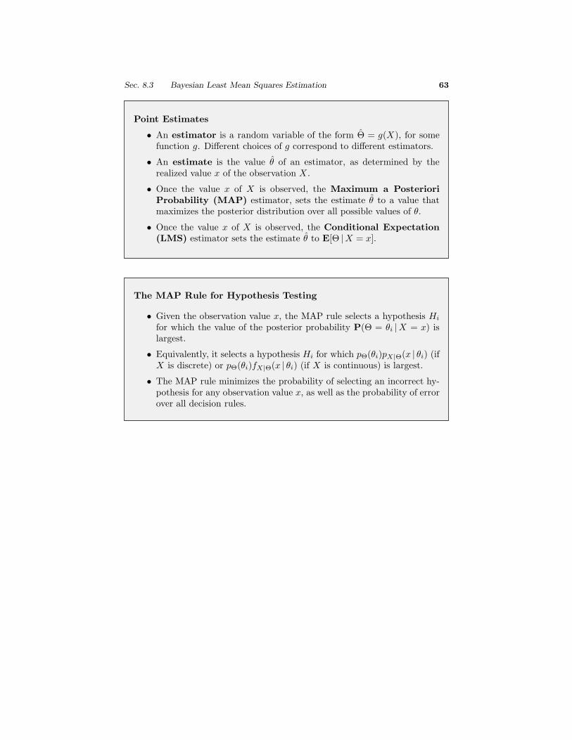
Point Estimates

• An estimator is a random variable of the form Θ = g(X), for somefunction g. Different choices of g correspond to different estimators.

• An estimate is the value θ of an estimator, as determined by therealized value x of the observation X .

• Once the value x of X is observed, the Maximum a PosterioriProbability (MAP) estimator, sets the estimate θ to a value thatmaximizes the posterior distribution over all possible values of θ.

• Once the value x of X is observed, the Conditional Expectation(LMS) estimator sets the estimate θ to E[Θ |X = x].

The MAP Rule for Hypothesis Testing

• Given the observation value x, the MAP rule selects a hypothesis Hi

for which the value of the posterior probability P(Θ = θi |X = x) islargest.

• Equivalently, it selects a hypothesis Hi for which pΘ(θi)pX|Θ(x | θi) (ifX is discrete) or pΘ(θi)fX|Θ(x | θi) (if X is continuous) is largest.

• The MAP rule minimizes the probability of selecting an incorrect hy-pothesis for any observation value x, as well as the probability of errorover all decision rules.


8.3 BAYESIAN LEAST MEAN SQUARES ESTIMATION

Key Facts About Least Mean Squares Estimation

• In the absence of any observations, E[

(Θ − θ)2]

is minimized when

θ = E[Θ]:

E[

(

Θ−E[Θ])2]

≤ E[

(Θ− θ)2]

, for all θ.

• For any given value x of X , E[

(Θ − θ)2 |X = x]

is minimized when

θ = E[Θ |X = x]:

E[

(

Θ−E[Θ |X = x])2 ∣∣ X = x

]

≤ E[

(Θ − θ)2 |X = x]

, for all θ.

• Out of all estimators g(X) of Θ based on X , the mean squared esti-

mation error E[

(

Θ− g(X))2]

is minimized when g(X) = E[Θ |X ]:

E[

(

Θ−E[Θ |X ])2]

≤ E[

(

Θ− g(X))2]

, for all estimators g(X).


Properties of the Estimation Error

• The estimation error Θ is unbiased, i.e., it has zero unconditionaland conditional mean:

E[Θ] = 0, E[Θ |X = x] = 0, for all x.

• The estimation error Θ is uncorrelated with the estimate Θ:

cov(Θ, Θ) = 0.

• The variance of Θ can be decomposed as

var(Θ) = var(Θ) + var(Θ).

8.4 BAYESIAN LINEAR LEAST MEAN SQUARES ESTIMATION

Linear LMS Estimation Formulas

• The linear LMS estimator Θ of Θ based on X is

Θ = E[Θ] +cov(Θ, X)

var(X)

(

X −E[X ])

= E[Θ] + ρσΘ

σX

(

X −E[X ])

,

where

ρ =cov(Θ, X)

σΘσX

is the correlation coefficient.

• The resulting mean squared estimation error is equal to

(1− ρ2)σ2Θ.


9

Classical Statistical Inference




Contents

9.1. Classical Parameter Estimation . . . . . . . . . . . . . . p. 4609.2. Linear Regression . . . . . . . . . . . . . . . . . . . . p. 4759.3. Binary Hypothesis Testing . . . . . . . . . . . . . . . . p. 4859.4. Significance Testing . . . . . . . . . . . . . . . . . . . p. 4959.5. Summary and Discussion . . . . . . . . . . . . . . . . p. 506

Problems . . . . . . . . . . . . . . . . . . . . . . . . p. 507

67


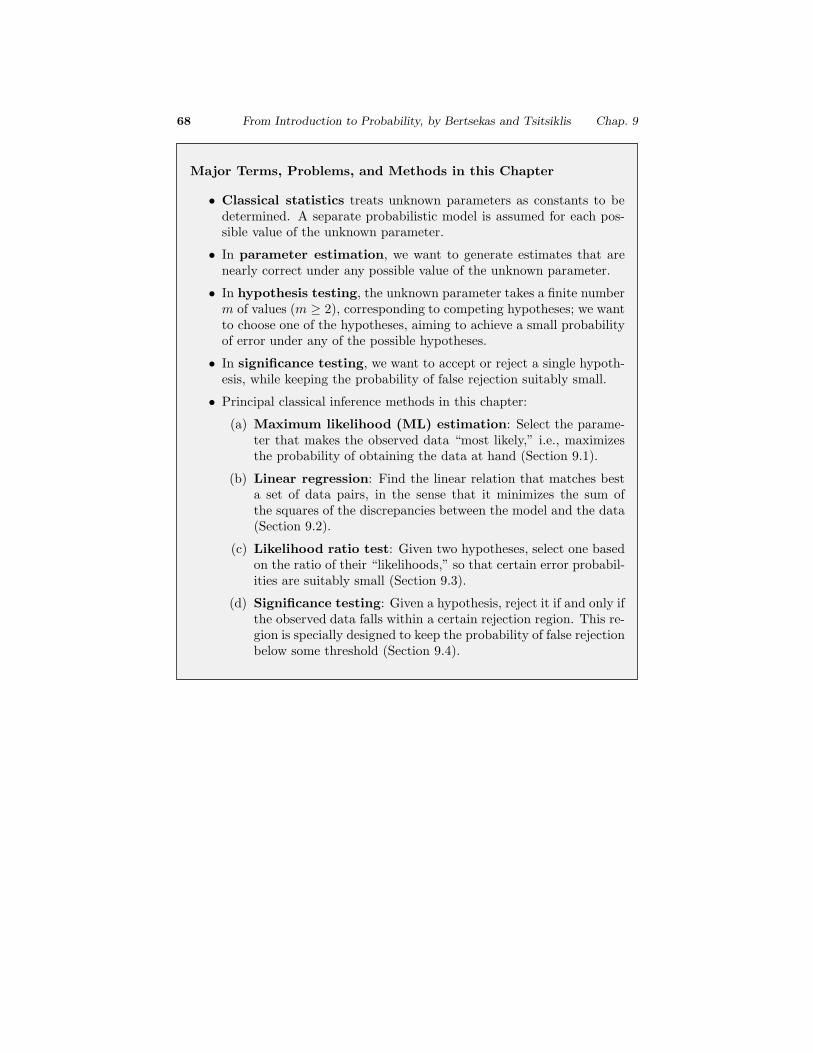
Major Terms, Problems, and Methods in this Chapter

• Classical statistics treats unknown parameters as constants to bedetermined. A separate probabilistic model is assumed for each pos-sible value of the unknown parameter.

• In parameter estimation, we want to generate estimates that arenearly correct under any possible value of the unknown parameter.

• In hypothesis testing, the unknown parameter takes a finite numberm of values (m ≥ 2), corresponding to competing hypotheses; we wantto choose one of the hypotheses, aiming to achieve a small probabilityof error under any of the possible hypotheses.

• In significance testing, we want to accept or reject a single hypoth-esis, while keeping the probability of false rejection suitably small.

• Principal classical inference methods in this chapter:

(a) Maximum likelihood (ML) estimation: Select the parame-ter that makes the observed data “most likely,” i.e., maximizesthe probability of obtaining the data at hand (Section 9.1).

(b) Linear regression: Find the linear relation that matches besta set of data pairs, in the sense that it minimizes the sum ofthe squares of the discrepancies between the model and the data(Section 9.2).

(c) Likelihood ratio test: Given two hypotheses, select one basedon the ratio of their “likelihoods,” so that certain error probabil-ities are suitably small (Section 9.3).

(d) Significance testing: Given a hypothesis, reject it if and only ifthe observed data falls within a certain rejection region. This re-gion is specially designed to keep the probability of false rejectionbelow some threshold (Section 9.4).

Sec. 9.1 Classical Parameter Estimation 69

9.1 CLASSICAL PARAMETER ESTIMATION

Terminology Regarding Estimators

Let Θn be an estimator of an unknown parameter θ, that is, a function ofn observations X1, . . . , Xn whose distribution depends on θ.

• The estimation error, denoted by Θn, is defined by Θn = Θn − θ.

• The bias of the estimator, denoted by bθ(Θn), is the expected valueof the estimation error:

bθ(Θn) = Eθ[Θn]− θ.

• The expected value, the variance, and the bias of Θn depend on θ,while the estimation error depends in addition on the observationsX1, . . . , Xn.

• We call Θn unbiased if Eθ[Θn] = θ, for every possible value of θ.

• We call Θn asymptotically unbiased if limn→∞ Eθ[Θn] = θ, forevery possible value of θ.

• We call Θn consistent if the sequence Θn converges to the true valueof the parameter θ, in probability, for every possible value of θ.

Maximum Likelihood Estimation

• We are given the realization x = (x1, . . . , xn) of a random vectorX = (X1, . . . , Xn), distributed according to a PMF pX(x; θ) or PDFfX(x; θ).

• The maximum likelihood (ML) estimate is a value of θ that maximizesthe likelihood function, pX(x; θ) or fX(x; θ), over all θ.

• The ML estimate of a one-to-one function h(θ) of θ is h(θn), where θnis the ML estimate of θ (the invariance principle).

• When the random variables Xi are i.i.d., and under some mild addi-tional assumptions, each component of the ML estimator is consistentand asymptotically normal.


Estimates of the Mean and Variance of a Random Variable

Let the observations X1, . . . , Xn be i.i.d., with mean θ and variance v thatare unknown.

• The sample mean

Mn =X1 + · · ·+Xn

n

is an unbiased estimator of θ, and its mean squared error is v/n.

• Two variance estimators are

S2n =

1

n

n∑

i=1

(Xi −Mn)2, S2n =

1

n− 1

n∑

i=1

(Xi −Mn)2.

• The estimator S2n coincides with the ML estimator if the Xi are nor-

mal. It is biased but asymptotically unbiased. The estimator S2n is

unbiased. For large n, the two variance estimators essentially coincide.

Confidence Intervals

• A confidence interval for a scalar unknown parameter θ is an intervalwhose endpoints Θ−

n and Θ+n bracket θ with a given high probability.

• Θ−n and Θ+

n are random variables that depend on the observationsX1, . . . , Xn.

• A 1− α confidence interval is one that satisfies

Pθ

(

Θ−n ≤ θ ≤ Θ+

n

)

≥ 1− α,

for all possible values of θ.

Sec. 9.2 Linear Regression 71

9.2 LINEAR REGRESSION

Linear Regression

Given n data pairs (xi, yi), the estimates that minimize the sum of thesquared residuals are given by

θ1 =

n∑

i=1

(xi − x)(yi − y)

n∑

i=1

(xi − x)2

, θ0 = y − θ1x,

where

x =1

n

n∑

i=1

xi, y =1

n

n∑

i=1

yi.


Bayesian Linear Regression

• Model:

(a) We assume a linear relation Yi = Θ0 +Θ1xi +Wi.

(b) The xi are modeled as known constants.

(c) The random variables Θ0,Θ1,W1, . . . ,Wn are normal and inde-pendent.

(d) The random variables Θ0 and Θ1 have mean zero and variancesσ20 , σ

21 , respectively.

(e) The random variables Wi have mean zero and variance σ2.

• Estimation Formulas:

Given the data pairs (xi, yi), the MAP estimates of Θ0 and Θ1 are

θ1 =σ21

σ2 + σ21

n∑

i=1

(xi − x)2

·n∑

i=1

(xi − x)(

yi − y)

,

θ0 =nσ2

0

σ2 + nσ20

(y − θ1x),

where

x =1

n

n∑

i=1

xi, y =1

n

n∑

i=1

yi.

9.3 BINARY HYPOTHESIS TESTING

Likelihood Ratio Test (LRT)

• Start with a target value α for the false rejection probability.

• Choose a value for ξ such that the false rejection probability is equalto α:

P L(X) > ξ;H0 = α.

• Once the value x of X is

(

observed, rejec

)

t H0 if L(x) > ξ.

Sec. 9.4 Significance Testing 73

Neyman-Pearson Lemma

Consider a particular choice of ξ in the LRT, which results in error proba-bilities

P(

L(X) > ξ;H0

)

= α, P(

L(X) ≤ ξ;H1

)

= β.

Suppose that some other test, with rejection region R, achieves a smaller orequal false rejection probability:

P(X ∈ R;H0) ≤ α.

Then,P(X /∈ R;H1) ≥ β,

with strict inequality P(X /∈ R;H1) > β when P(X ∈ R;H0) < α.


9.4 SIGNIFICANCE TESTING

Significance Testing Methodology

A statistical test of a hypothesis H0 is to be performed, based on the obser-vations X1, . . . , Xn.

• The following steps are carried out before the data are observed.

(a) Choose a statistic S, that is, a scalar random variable thatwill summarize the data to be obtained. Mathematically, thisinvolves the choice of a function h : ℜn → ℜ, resulting in thestatistic S = h(X1 . . . , Xn).

(b) Determine the shape of the rejection region by specifyingthe set of values of S for which H0 will be rejected as a functionof a yet undetermined critical value ξ.

(c) Choose the significance level, i.e., the desired probability α ofa false rejection of H0.

(d) Choose the critical value ξ so that the probability of false re-jection is equal (or approximately equal) to α. At this point, therejection region is completely determined.

• Once the values x1, . . . , xn of X1, . . . , Xn are observed:

(i) Calculate the value s = h(x1, . . . , xn) of the statistic S.

(ii) Reject the hypothesis H0 if s belongs to the rejection region.


The Chi-Square Test:

• Use the statistic

S =m∑

k=1

Nk log( Nk

nθ∗k

)

(or possibly the related statistic T ) and a rejection region of the form

reject H0 if 2S > γ

(or T > γ, respectively).

• The critical value γ is determined from the CDF tables for the χ2

distribution with m− 1 degrees of freedom so that

P(2S > γ;H0) = α,

where α is a given significance level.


MIT OpenCourseWarehttps://ocw.mit.edu

Resource: Introduction to ProbabilityJohn Tsitsiklis and Patrick Jaillet

The following may not correspond to a p articular course on MIT OpenCourseWare, but has beenprovided by the author as an individual learning resource.

For information about citing these materials or our Terms of Use, visit: https://ocw.mit.edu/terms.

https://ocw.mit.edu

https://ocw.mit.edu/terms

Date post:	21-May-2020
Category:	Documents
Upload:	others
View:	45 times
Download:	1 times

Introduction to Probability, Selected Textbook Summary ... · 6 From Introduction to Probability,...

Documents