252
Introduction to Programming in ATS Hongwei Xi ATS Trustful Software, Inc.

Introduction to Programming in ATS
Hongwei XiATS Trustful Software, Inc.

Introduction to Programming in ATSby Hongwei Xi
Copyright © 2010-201? Hongwei Xi
As a programming language, ATS is both syntax-rich and feature-rich. This book introduces the reader to some corefeatures of ATS, including basic functional programming, simple types, (recursively defined) datatypes, polymorphictypes, dependent types, linear types, theorem-proving, programming with theorem-proving (PwTP), andtemplate-based programming. Although the reader is not assumed to be familiar with programming in general, thebook is likely to be rather dense for someone without considerable programming experience.
All rights are reserved. Permission is granted to print this document for personal use.

Dedication
To Jinning, Zoe, and Chloe.

Table of ContentsPreface ..................................................................................................................................................... viiI. Basic Functional Programming ...........................................................................................................ix
1. Preparation for Starting ..................................................................................................................11.1. A Running Program...........................................................................................................11.2. A Template for Single-File Programs................................................................................11.3. A Makefile Template .........................................................................................................2
2. Elements of Programming .............................................................................................................52.1. Expressions and Values .....................................................................................................52.2. Names and Bindings..........................................................................................................62.3. Scopes for Bindings...........................................................................................................62.4. Environments for Evaluation.............................................................................................72.5. Static Semantics.................................................................................................................82.6. Primitive Types ..................................................................................................................82.7. Tuples and Tuple Types .....................................................................................................92.8. Records and Record Types ..............................................................................................102.9. Conditional Expressions..................................................................................................112.10. Sequence Expressions ...................................................................................................122.11. Comments in Code ........................................................................................................13
3. Functions ......................................................................................................................................143.1. Functions as a Simple Form of Abstraction ....................................................................143.2. Function Arity .................................................................................................................153.3. Function Interface............................................................................................................163.4. Evaluation of Function Calls ...........................................................................................173.5. Recursive Functions ........................................................................................................173.6. Evaluation of Recursive Function Calls ..........................................................................183.7. Example: Coin Changes for Fun .....................................................................................193.8. Tail-Call and Tail-Recursion............................................................................................203.9. Example: The Eight-Queens Puzzle................................................................................213.10. Mutually Recursive Functions.......................................................................................253.11. Mutually Defined Tail-Recursion ..................................................................................253.12. Envless Functions and Closure-Functions.....................................................................273.13. Higher-Order Functions.................................................................................................293.14. Example: Binary Search for Fun ...................................................................................313.15. Example: A Higher-Order Fun Puzzle ..........................................................................313.16. Currying and Uncurrying ..............................................................................................32
4. Datatypes......................................................................................................................................344.1. Patterns ............................................................................................................................344.2. Pattern-Matching .............................................................................................................344.3. Matching Clauses and Case-Expressions ........................................................................354.4. Enumerative Datatypes....................................................................................................364.5. Recursively Defined Datatypes .......................................................................................374.6. Exhaustiveness of Pattern-Matching ...............................................................................384.7. Example: Binary Search Tree..........................................................................................394.8. Example: Evaluating Integer Expressions .......................................................................41
5. Parametric Polymorphism............................................................................................................455.1. Function Templates .........................................................................................................45
iv

5.2. Polymorphic Functions....................................................................................................475.3. Polymorphic Datatypes ...................................................................................................485.4. Example: Function Templates on Lists ...........................................................................505.5. Example: Mergesort on Lists...........................................................................................54
II. Support for Practical Programming.................................................................................................576. Effectful Programming Features ..................................................................................................58
6.1. Exceptions .......................................................................................................................586.2. Example: Testing for Braun Trees...................................................................................606.3. References .......................................................................................................................636.4. Example: A Counter Implementation..............................................................................646.5. Arrays ..............................................................................................................................656.6. Example: Ordering Permutations ....................................................................................666.7. Matrices ...........................................................................................................................696.8. Example: Estimating the Constant Pi ..............................................................................716.9. Simple Input and Output .................................................................................................71
7. Modularity....................................................................................................................................757.1. Types as a Form of Specification.....................................................................................757.2. Static and Dynamic ATS Files.........................................................................................777.3. Generic Template Implementation ..................................................................................807.4. Specific Template Implementation ..................................................................................817.5. Abstract Types .................................................................................................................827.6. Example: A Package for Rationals..................................................................................857.7. Example: A Functorial Package for Rationals ................................................................86
8. Interaction with C.........................................................................................................................908.1. External Global Names....................................................................................................908.2. External Types and Values in ATS ..................................................................................928.3. Inclusion of External Code in ATS..................................................................................928.4. Calling External Functions in ATS..................................................................................938.5. Unsafe C-style Programming in ATS..............................................................................948.6. Exporting Types in ATS for Use in C..............................................................................978.7. Example: Constructing a Statically Allocated List .........................................................98
III. Programming with Dependent Types............................................................................................1019. Introduction to Dependent Types ...............................................................................................102
9.1. Enhanced Expressiveness for Specification ..................................................................1029.2. Constraint-Solving during Typechecking......................................................................1059.3. Example: String Processing...........................................................................................1069.4. Example: Binary Search on Arrays ...............................................................................1099.5. Termination-Checking for Recursive Functions............................................................1119.6. Example: Dependent Types for Debugging...................................................................112
10. Datatype Refinement................................................................................................................11510.1. Dependent Datatypes...................................................................................................11510.2. Example: Function Templates on Lists (Redux) .........................................................11810.3. Example: Mergesort on Lists (Redux).........................................................................12110.4. Sequentiality of Pattern Matching ...............................................................................12310.5. Example: Functional Red-Black Trees........................................................................124
11. Theorem-Proving in ATS/LF ...................................................................................................12911.1. Encoding Relations as Dataprops................................................................................129
v

11.2. Constructing Proofs as Total Functions.......................................................................13011.3. Example: Distributivity of Multiplication ...................................................................13211.4. Example: Commutativity of Multiplication ................................................................13311.5. Algebraic Datasorts .....................................................................................................13511.6. Example: Establishing Properties on Braun Trees ......................................................13811.7. Programmer-Centric Theorem-Proving.......................................................................141
12. Programming with Theorem-Proving ......................................................................................14412.1. Circumventing Nonlinear Constraints .........................................................................14412.2. Example: Safe Matrix Subscripting.............................................................................14512.3. Specifying with Enhanced Precision ...........................................................................14712.4. Example: Another Verified Factorial...........................................................................14812.5. Example: Verified Fast Exponentiation .......................................................................150
IV. Programming with Views and Viewtypes .....................................................................................15413. Introduction to Views and Viewtypes ......................................................................................155
13.1. Views for Memory Access through Pointers ...............................................................15513.2. Viewtypes as a Combination of Views and Types.......................................................15813.3. Left-Values and Call-by-Reference .............................................................................15913.4. Stack-Allocated Variables ...........................................................................................16113.5. Heap-Allocated Linear Closure-Functions..................................................................163
14. Dataviews as Linear Dataprops................................................................................................16614.1. Optional Views ............................................................................................................16614.2. Disjunctive Views........................................................................................................16614.3. Dataview for Linear Arrays .........................................................................................16814.4. Dataview for Linear Strings.........................................................................................17114.5. Dataview for Singly-Linked Lists ...............................................................................17414.6. Proof Functions for View-Changes .............................................................................178
15. Dataviewtypes as Linear Datatypes .........................................................................................18415.1. Linear Optional Values ................................................................................................18415.2. Linear Lists ..................................................................................................................18515.3. Example: Merge-Sort on Linear Lists .........................................................................19115.4. Example: Insertion Sort on Linear Lists......................................................................19315.5. Example: Quick-Sort on Linear Lists..........................................................................19615.6. Linear Binary Search Trees .........................................................................................19915.7. Transition from Datatypes to Dataviewtypes ..............................................................204
16. Abstract Views and Viewtypes.................................................................................................20916.1. Simple Linear Objects .................................................................................................20916.2. Memory Allocation and Deallocation .........................................................................21316.3. Example: Array-Based Circular Buffers .....................................................................21716.4. Locking and Unlocking ...............................................................................................21916.5. Linear Channels for Asynchronous IPC......................................................................223
V. Programming with Function Templates .........................................................................................22917. From Genericity to Late-Binding.............................................................................................230
17.1. Genericity of Template Implementations ....................................................................23017.2. Example: Generic Operations on Numbers.................................................................23217.3. Templates as a Special Form of Functors ....................................................................23517.4. Example: Templates for Loop Construction................................................................23717.5. Template-Based Support for Late-Binding..................................................................241
vi

Preface
ATS (http://www.ats-lang.org) is a statically typed programming language that unifies implementationwith formal specification. Within ATS, there are two sublanguages: one for specification and the other forimplementation, and there is also a theorem-proving subsystem for verifying whether an implementationindeed implements according to its specification. If I could associate only one single word with ATS, Iwould choose the word precision. Programming in ATS is about being precise and being able toeffectively enforce precision. This point will be demonstrated concretely and repeatedly in this book.
In order to be precise in building software systems, we need to specify what such a system is expected toaccomplish. In the current day and age, software specification, which is used in a rather loose sense here,is often done in forms of varying degrees of formalism, ranging from verbal discussions to pencil/paperdrawings to diagrammatic depictions in modeling languages such as UML to text descriptions in formalspecification languages such as VDM and Z. Often the main purpose of software specification is toestablish some mutual understanding among a team of developers. After the specification for a softwaresystem is done, either formally or informally, we need to implement the specification in a programminglanguage. In general, it is exceedingly difficult to be reasonably certain whether an implementationactually meets its specification. Even if the implementation coheres well with its specification initially, itnearly inevitably diverges from the specification as the software system evolves. The dreadfulconsequences of such a divergence are all too familiar; the specification becomes less and less reliablefor understanding the behavior of the software system while the implementation gradually turns into itsown specification; for the developers, it becomes increasingly difficult and risky to maintain and extendthe software system; for the users, it requires increased amount of time and effort to learn and use thesoftware system.
Largely inspired by Martin-Loef’s constructive type theory, which was originally developed for thepurpose of establishing a foundation for mathematics, I designed ATS in an attempt to combinespecification and implementation into a single programming language. There are a static component(statics) and a dynamic component (dynamics) in ATS. Intuitively, the statics and dynamics are each forhandling types and programs, respectively. In particular, specification is done in the statics. Given aspecification, how can we then effectively ensure that an implementation of the specification (type)indeed implements according to the specification? We request that the programmer who does theimplementation also construct a proof in the theorem-proving subsystem of ATS to demonstrate it. Thisis a style of program verification that puts the programmer at the center, and thus we refer to it as aprogrammer-centric approach to program verification.
As a programming language, ATS is both syntax-rich and feature-rich. It can support a variety ofprogramming paradigms, including functional programming, imperative programming, object-orientedprogramming, concurrent programming, modular programming, etc. However, the core of ATS, which isbased on a call-by-value functional language, is surprisingly simple, and this is where the journey ofprogramming in ATS starts. In this book, I will demonstrate primarily through examples how variousprogramming features in ATS can be employed effectively to facilitate the construction of high-qualityprograms. I will focus on programming practice instead of programming theory. If you are primarilyinterested in the type-theoretical foundation of ATS, then you have to find it elsewhere.
vii

Preface
If you can implement, then you are a good programmer. In order to be a better programmer, you shouldalso be able to explain what you implement. If you can guarantee what is implemented matches what isspecified, then you are surely the best programmer. Hopefully, learning ATS will put you on a wonderfulexploring journey to become the best programmer. Let that journey start now!
viii

I. Basic Functional Programming

Chapter 1. Preparation for Starting
It is likely that you want to write programs in the programming language you are learning. You may alsowant to try some of the examples included in this book and see what really happens. So I will first showyou how to write in ATS a single-file program, that is, a program contained in a single file, and compile itand then execute it.
1.1. A Running Program
The following example is a program in ATS that prints out (onto the console) the string "Hello, world!"plus a newline before it terminates:
//val _ = print ("Hello, world!\n")//implement main0 () = () // a dummy for [main]//
The keyword val initiates a binding between the variable _ (underscore) and the function call print("Hello, world!\n"). However, this binding is never used after it is introduced; its sole purpose is for thecall to the print function to get evaluated.
The function main0 is a slight variant of another function named main, which is of certain specialmeaning in ATS. For a programmer who knows the C or Java programming language, I simply point outthat the role of main is essentially the same as its counterpart of the same name in C or Java. Thekeyword implement initiates the implementation of a function whose interface has already been declaredelsewhere. Following is the declared interface for main0 in ATS:
fun main0 (): void
which indicates that main0 is a nullary function, that is, a function taking no arguments, and it returns novalue (or it returns the void value). The double slash symbol (//) initiates a comment that terminates atthe end of the current line.
Suppose that you have already installed the ATS programming language system. You can issue thefollowing command-line to generate an executable named hello in the current working directory:
atscc -o hello hello.dats
where hello.dats refers to a file containing the above program. The command atscc is essentially aconvenience wrapper around the command atsopt, which triggers the process of typechecking andcompiling ATS programs. Note that atscc and atsopt may actually be given the names patscc andpatsopt, respectively, in certain installations of ATS. The filename extension .dats should not be alteredas it has already been assigned a special meaning that the compilation command atscc recognizes.Another special filename extension is .sats, which we will soon encounter.
1

Chapter 1. Preparation for Starting
1.2. A Template for Single-File Programs
The following code template, which is available on-line (https://github.com/ats-lang/ats-lang.github.io/blob/master/DOCUMENT/INT2PROGINATS/CODE/CHAP_START/mytest.dats), isdesigned for constructing a single-file program in ATS:
(***** A template for single-file ATS programs
***)
(* ****** ****** *)//#include "share/atspre_define.hats"#include "share/atspre_staload.hats"//(* ****** ****** *)
//// please write you program in this section//
(* ****** ****** *)
implement main0 () = () // a dummy implementation for [main]
The line starting with the keyword #include enables the ATS compiler atsopt to gain access to certainexternal library packages and the definitions of various library functions. I will cover elsewhere in thebook the topic on making use of library code in ATS.
1.3. A Makefile Template
The following Makefile template, which is available on-line (https://github.com/ats-lang/ats-lang.github.io/blob/master/DOCUMENT/INT2PROGINATS/CODE/CHAP_START/Makefile_template),is provided to help you construct your own Makefile for compiling ATS programs. If you are not familiarwith the make utility, you could readily find plenty resources on-line to help yourself learn it.
######## Note that# certain installations require the following changes:## atscc -> patscc# atsopt -> patsopt# ATSHOME -> PATSHOME#
2

Chapter 1. Preparation for Starting
#######ATSHOMEQ="$(ATSHOME)"########ATSCC=$(ATSHOMEQ)/bin/atsccATSOPT=$(ATSHOMEQ)/bin/atsopt########## HX: Please uncomment the one you want, or skip it entirely#ATSCCFLAGS=# ATSCCFLAGS=-O2## ’-flto’ enables link-time optimization such as inlining lib functions## ATSCCFLAGS=-O2 -flto#########cleanall::######### Please uncomment the following three lines and replace the name [foo]# with the name of the file you want to compile## foo: foo.dats ; \# $(ATSCC) $(ATSCCFLAGS) -o $@ $< || echo $@ ": ERROR!!!"# cleanall:: ; $(RMF) foo######### You may find these rules useful## %_sats.o: %.sats ; $(ATSCC) $(ATSCCFLAGS) -c $< || echo $@ ": ERROR!!!"# %_dats.o: %.dats ; $(ATSCC) $(ATSCCFLAGS) -c $< || echo $@ ": ERROR!!!"########RMF=rm -f########clean:: ; $(RMF) *~clean:: ; $(RMF) *_?ats.oclean:: ; $(RMF) *_?ats.c#cleanall:: clean
3

Chapter 1. Preparation for Starting
####### end of [Makefile] ######
4

Chapter 2. Elements of Programming
The core of ATS is a call-by-value functional programming language. I will explain the meaning ofcall-by-value in a moment. As for functional programming, there is really no precise definition. Themost important aspect of functional programming that I want to explore is the notion of binding, whichrelates names to expressions.
2.1. Expressions and Values
ATS is both syntax-rich and feature-rich, and its grammar is probably more complex than most existingprogramming languages. In ATS, there are a large variety of forms of expressions, which I will introducegradually.
Let us first start with some integer arithmetic expressions (IAEs): 1, ~2, 1+2, 1+2*3-4, (1+2)/(3-4), etc.Note that the negative sign is represented by the tilde symbol (~) in ATS. There is also support forfloating point numbers, and some floating point constants are given here: 1.0, ~2.0, 3., 0.12345, 2.71828,31416E-4, etc. Note that 3. and 31416E-4 are the same as 3.0 and 3.1416, respectively. What I reallywant to emphasize at this point is that 1 and 1.0 are two distinct numbers in ATS: the former is an integerwhile the latter is a floating point number (of double precision).
There are also boolean constants: true and false. We can form boolean expressions such as 1 >= 0,not(2-1 >= 2), (1 < 2) andalso (2 < 3) and (~1 > 1) orelse (~1 <= 1), where not, andalso and orelse standfor negation, conjunction and disjunction, respectively. For programmers familiar with C-like syntax, Ipoint out that operators && and || are synonyms for andalso and orelse, respectively.
Other commonly used constant values include characters and strings. For instance, following are somecharacter constants: ’a’, ’B’, ’\n’ (newline), ’\t’ (tab), ’\(’ (left parenthesis), ’)’ (right parenthesis), ’\{’(left curly brace), ’}’ (right curly brace), etc; following are some string constants: "My name is Zoe","Don’t call me \"Chloe\"", "this is a newline:\n", etc.
Given a (function) name, say, foo, and an expression exp, the expression foo(exp) is a functionapplication or function call. The parentheses in foo(exp) may be dropped if no ambiguity is created bydoing so. For instance, print("Hello") is a function application, which can also be written as print"Hello". If foo is a nullary function, then a function application foo() can be formed. If foo is a binaryfunction, then a function application foo(exp1, exp2) can be formed for expressions exp1 and exp2.Functions of more arguments can be treated accordingly.
Note that we cannot write +(1,2) as the name + has already been given the infix status requiring that it betreated as an infix operator. However, we can write op+(1,2), where op is a keyword in ATS that can beused to temporarily suspend the infix status of any name immediately following it. I will explain in detailthe issue of fixity (prefix, infix and postfix) elsewhere.
5

Chapter 2. Elements of Programming
Values are essentially expressions of certain special forms, which cannot be reduced or simplified further.For instance, integer constants such as 1 and ~2 are values, but the integer expression 1+2 is not a value,which can be reduced to the value 3. Evaluation refers to the computational process that reduces a givenexpression into a value. However, certain expressions such as 1/0 cannot be reduced to a value, andevaluating such an expression must abort at some point. I will gradually present more information onevaluation.
2.2. Names and Bindings
A crucial aspect of a programming language is the mechanism it provides for binding names, which arethemselves expressions, to expressions. For instance, a declaration is introduced by the following syntaxthat declares a binding between the name x, which is also referred to as a variable, and the expression1+2:
val x = 1 + 2
Note that val is a keyword in ATS, and the declaration is classified as a val-declaration. Conceptually,what happens at run-time in a call-by-value language such as ATS is that the expression 1+2 is firstevaluated to the value 3, and then the binding between x and 1+2 is finalized into a binding between xand 3. Essentially, call-by-value means that a binding between a name and an expression needs to befinalized into one between the name and the value of the expression before it can be used in evaluationsubsequently. As another example, the following syntax declares three bindings, two of which areformed simultaneously in the first line:
val PI = 3.14 and radius = 10.0val area = PI * radius * radius
Note that it is unspecified in ATS as to which of the first two bindings (connected by the keyword and) isfinalized ahead of the other at run-time. However, it is guaranteed that the third binding is finalized afterthe first two are done. To see this issue from a different angle, we can try to typecheck the followingcode:
val x = 0 and y = x + 1
The error message reported in this case indicates that the name (or dynamic identifier) x in the expressionx + 1 is unbound. In particular, the two occurrences of x in the above code are unrelated.
2.3. Scopes for Bindings
Each binding is given a fixed scope in which the binding is considered legal or effective. The scope of atoplevel binding in a file starts from the point where the binding is introduced until the very end of thefile. The bindings introduced in the following example between the keywords let and in are effective untilthe keyword end is reached:
6

Chapter 2. Elements of Programming
val area = letval PI = 3.14 and radius = 10.0 in PI * radius * radius
end // end of [let]
Such bindings are referred to as local bindings, and the names such as PI and radius are referred to aslocal names. This example can also be written in the following style:
val area =PI * radius * radius where {val PI = 3.14 and radius = 10.0 // simultaneous bindings
} // end of [where] // end of [val]
The keyword where appearing immediately after an expression introduces bindings that are solelyeffective for evaluating names contained in the expression. Note that expressions formed using thekeywords let and where are often referred to as let-expressions and where-expressions, respectively. Theformer can always be translated into the latter directly and vice versa. Which style is better? I have notformed my opinion yet. The answer seems to entirely depend on the taste of the programmer.
The following example demonstrates an alternative approach to introducing local bindings:
local
val PI = 3.14 and radius = 10.0
in (* in-of-local *)
val area = PI * radius * radius
end // end of [local]
where the bindings introduced between the keywords local and in are effective until the keyword end isreached. Note that the bindings introduced between the keywords in and end are themselves toplevelbindings. The difference between let and local should be clear: The former is used to form an expressionwhile the latter is used to introduce a sequence of declarations.
2.4. Environments for Evaluation
Evaluation is the computational process that reduces expressions to values. When performing evaluation,we need not only the expression to be evaluated but also a collection of bindings that map names in theexpression to values. This collection of bindings, which is just a finite mapping, is often referred to as anenvironment (for evaluation). For instance, suppose that we want to evaluate the following expression:
letval PI = 3.14 and radius2 = 10.0 * 10.0 in PI * radius2
end
7

Chapter 2. Elements of Programming
We start with the empty environment ENV0; we evaluate 3.14 to itself and 10.0 * 10.0 to 100.0 under theenvironment ENV0; we then extend ENV0 to ENV1 with two bindings mapping PI to 3.14 and radius2to 100.0; we then evaluate PI * radius2 under ENV1 to 3.14 * radius2, then to 3.14 * 100.0, and finally to314.0, which is the value of the let-expression.
2.5. Static Semantics
ATS is a programming language equipped with a highly expressive type system rooted in the AppliedType System framework, which also gives ATS its name. I will gradually introduce the type system ofATS, which is probably the most outstanding and interesting part of this book.
It is common to treat a type as the set of values it classifies. However, I find it more approriate to treat atype as a form of meaning. There are formal rules for assigning types to expressions, which are referredto as typing rules. If a type T can be assigned to an expression, then I say that the expression possessesthe static meaning (semantics) represented by the type T. Note that an expression may be assigned manydistinct static meanings. An expression is well-typed if there exists a type T such that the expression canbe assigned the type T.
If there is a binding between a name and an expression and the expression is of some type T, then thename is assumed to be of the type T in the effective scope of the binding. In other words, the nameassumes the static meaning of the expression it refers to.
Let exp0 be an expression of some type T, that is, the type T can be assigned to exp0 according to certaintyping rules. If we can evaluate exp0 to exp1, then exp1 can also be assigned the type T. In other words,static meaning is an invariant under evaluation. This property is often referred to as type preservation,which is part of the soundness of the type system of ATS. Based on this property, we can readily inferthat any value is of the type T if exp0 can be evaluated to it (in multiple steps).
Let exp0 be an expression of some type T. Assume that exp0 is not a value. Then exp0 can always beevaluated one step further to another expression exp1. This property is often referred to as progress,which is another part of the soundness of the type system of ATS.
2.6. Primitive Types
The simplest types in ATS are primitive types, which are used to classify primitive values. For instance,we have the primitive types int and double, which classify integers (in a fixed range) and floating pointnumbers (of double precision), respectively.
In the current implementation of ATS (Postiats), a program in ATS is first compiled into one in C(conforming to the C99 standard), which can then be compiled to object code by a compiler for C such
8

Chapter 2. Elements of Programming
as gcc. In the compilation from ATS to C, each of the types int, double and void in ATS is translated tothe type of the same name in C.
There are many other primitive types in ATS, and I will introduce them gradually. Some commonly usedprimitive types are listed as follows:
• bool: This type is for boolean values true and false, and it is translated into the int type in C.
• char: This type is translated into the type in C for characters.
• schar: This type is translated into the type in C for signed characters.
• uchar: This type is translated into the type in C for unsigned characters.
• float: This type is translated into the type in C for floating point numbers of single precision.
• uint: This type is translated into the type in C for unsigned integers.
• lint: This type is translated into the type in C for long integers.
• ulint: This type is translated into the type in C for unsigned long integers.
• llint: This type is translated into the type in C for long long integers.
• ullint: This type is translated into the type in C for unsigned long long integers.
• size_t: This type is translated into the type in C of the same name, which is for unsigned integers ofcertain precision. Usually, the type size_t can be treated as the type ulint and vice versa.
• ssize_t: This type is translated into the type in C of the same name, which is for signed integers ofcertain precision. Usually, the type ssize_t can be treated as the type lint and vice versa.
• sint: This type is translated into the type in C for short integers.
• usint: This type is translated into the type in C for unsigned short integers.
• string: This type is for strings, and its translation in C is the type for pointers. I will explain thistranslation elsewhere.
I will gradually present programming examples involving various primitive types and values.
2.7. Tuples and Tuple Types
Given two types T1 and T2, we can form a tuple type (T1, T2), which can also be written as @(T1, T2).Assume that exp1 and exp2 are two expressions of the types T1 and T2, respectively. Then theexpression (exp1, exp2), which can also be written as @(exp1, exp2), refers to a tuple of the tuple type(T1, T2). Accordingly, we can form tuples and tuple types of more components. In order for a tuple typeto be assigned to a tuple, the tuple and the tuple type must have the equal number of components.
When evaluating a tuple expression, we evaluate all of its components sequentially. Suppose that theexpression contains n components, then the value of the expression is the tuple consisting of the n valuesof the n components listed in the order as the components themselves.
9

Chapter 2. Elements of Programming
A tuple of length n for n >= 2 is just a record of field names ranging from 0 until n-1, inclusive. Given anexpression exp of some tuple type (T1, T2), we can form expressions (exp).0 and (exp).1, which are oftypes T1 and T2, respectively. Note that the expression exp does not have to be a tuple expression. Forinstance, exp may be a name or a function application. If exp evaluates to a tuple of two values, thenexp.0 evaluates to the first value and exp.1 the second value. Clearly, if the tuple type of exp containsmore components, what is stated can be generalized accordingly.
In the following example, we first construct a tuple of length 3 and then introduce bindings between 3names and all of the 3 components of the tuple:
val xyz = (’A’, 1, 2.0)val x = xyz.0 and y = xyz.1 and z = xyz.2
Note that the constructed tuple can be assigned the tuple type (char, int, double). Another method forselecting components in a given tuple is based on pattern matching, which is employed in the followingexample:
val xyz = (’A’, 1, 2.0)val (x, y, z) = xyz // x = ’A’; y = 1; z = 2.0
Note that (x, y, z) is a pattern that can match any tuples of exact 3 components. I will say more aboutpattern matching elsewhere.
The tuples introduced above are often referred to as flat tuples, native tuples or unboxed tuples. There isanother kind of tuples supported in ATS, which are called boxed tuples. A boxed tuple is essentially apointer pointing to some heap location where a flat tuple is stored.
Assume that exp1 and exp2 are two expressions of the types T1 and T2, respectively. Then theexpression ’(exp1, exp2), refers to a tuple of the tuple type ’(T1, T2). Accordingly, we can form boxedtuples and boxed tuple types of fewer or more components. What should be noted immediately is thatevery boxed tuple is of the size of a pointer, and can thus be stored in any place where a pointer can.Using boxed tuples is rather similar to using unboxed ones. For instance, the meaning of the followingcode should be evident:
val xyz = ’( ’A’, 1, 2.0 )val x = xyz.0 and y = xyz.1 and z = xyz.2
Note that a space is needed between ’( and ’A’ for otherwise the current parser (for ATS/Postiats) wouldbe confused.
Given the availability of flat and boxed tuples, one naturally wants to know whether there is a simple wayto determine which kind is preferred over the other. Unfortunately, there is no simple way to do this asfar as I can tell. In order to be certain, some kind of profiling is often needed. However, if we want to runcode with no support of garbage collection (GC), then we should definitely avoid using boxed tuples.
10

Chapter 2. Elements of Programming
2.8. Records and Record Types
A record is just like a tuple except that each field name of the record is chosen by the programmer(instead of being fixed). Similarly, a record type is just like a tuple type. For instance, a record typepoint2D is defined as follows:
typedefpoint2D = @{ x= double, y= double }
where x and y are the names of the two fields in a record value of this type. We also refer to a field in arecord as a component. The special symbol @{ indicates that the formed type is for flat/native/unboxedrecords. A value of the type point2D is constructed as follows and given the name theOrigin:
val theOrigin = @{ x= 0.0, y= 0.0 } : point2D
We can use the standard dot notation to extract out a selected component in a record, and this is shown inthe next line of code:
val theOrigin_x = theOrigin.x and theOrigin_y = theOrigin.y
Alternatively, we can use pattern matching for doing component extraction as is done in the next line ofcode:
val @{ x= theOrigin_x, y= theOrigin_y } = theOrigin
In this case, the names theOrigin_x and theOrigin_y are bound to the components in theOrgin that arenamed x and y, respectively. If we only need to extract out a selected few of components (instead of allthe available ones), we can make use of the following kind of patterns:
val @{ x= theOrigin_x, ... } = theOrigin // the x-component onlyval @{ y= theOrigin_y, ... } = theOrigin // the y-component only
If you find all this syntax for component extraction to be confusing, then I suggest that you stick to thedot notation. I myself rarely use pattern matching on record values.
Compared with handling native/flat/unboxed records, the only change needed for handling boxed recordsis to replace the special symbol @{ with another one: ’{, which is a quote followed immediately by a leftcurly brace.
11

Chapter 2. Elements of Programming
2.9. Conditional Expressions
A conditional expression consists of a test and two branches. For instance, the following expression isconditional:
if (x >= 0) then x else ~x
where if, then and else are keywords in ATS. In a conditional expression, the expression following if isthe test and the expressions following then and else are referred to as the then-branch and the else-branch(of the conditional expression), respectively.
In order to assign a type T to a conditional expression, we need to assign the type bool to the test and thetype T to both of the then-branch and the else-branch. For instance, the type int can be assigned to theabove conditional expression if the name x is given the type int.
Suppose that we have a conditional expression that is well-typed. When evaluating it, we first evaluatethe test to a value, which is guaranteed to be either true or false; if the value is true, then we continue toevaluate the then-branch; otherwise, we continue to evaluate the else-branch.
It is also allowed to form a conditional expression where the else-branch is missing or truncated. Forinstance, we can form an expression as follows:
if (x >= 0) then print(x)
which is equivalent to the following conditional expression:
if (x >= 0) then print(x) else ()
Note that () stands for the void value (of the type void). If a type can be assigned to a conditionalexpression in the truncated form, then the type must be void.
2.10. Sequence Expressions
Assume that exp1 and exp2 are expressions of types T1 and T2 respectively, where T1 is void. Then asequence expression (exp1; exp2) can be formed that is of the type T2. When evaluating the sequenceexpression (exp1; exp2), we first evaluate exp1 to the void value and then evaluate exp2 to some value,which is also the value of the sequence expression. When more expressions are sequenced, all of thembut the last one need to be of the type void and the type of the last expression is also the type of thesequence expression being formed. Evaluating a sequence of more expressions is analogous to evaluatinga sequence of two. The following example is a sequence expression:
(print ’H’; print ’e’; print ’l’; print ’l’; print ’o’)
12

Chapter 2. Elements of Programming
Evaluating this sequence expression prints out (onto the console) the 5-letter string "Hello". Instead ofparentheses, we can also use the keywords begin and end to form a sequence expression:
beginprint ’H’; print ’e’; print ’l’; print ’l’; print ’o’
end // end of [begin]
If we like, we may also add a semicolon immediately after the last expression in a sequence as long asthe last expression is of the type void. For instance, the above example can also be written as follows:
beginprint ’H’; print ’e’; print ’l’; print ’l’; print ’o’;
end // end of [begin]
I also want to point out the following style of sequencing:
letval () = print ’H’val () = print ’e’val () = print ’l’val () = print ’l’val () = print ’o’
in// nothing
end // end of [let]
which is quite common in functional programming.
2.11. Comments in Code
ATS currently supports four forms of comments: line comment, block comment of ML-style, blockcomment of C-style, and rest-of-file comment.
• A line comment starts with the double slash symbol (//) and extends until the end of the current line.
• A block comment of ML-style starts and closes with the tokens (* and *), respectively. Note thatnested block comments of ML-style are allowed, that is, one block comment of ML-style can occurwithin another one of the same style.
• A block comment of C-style starts and closes with the tokens /* and */, respectively. Note that blockcomments of C-style cannot be nested. The use of block comments of C-style is primarily in code thatis supposed to be shared by ATS and C. In other cases, block comments of ML-style should be thepreferred choice.
• A rest-of-file comment starts with the quadruple slash symbol (////) and extends until the end of thefile. Comments of this style of are primarily useful for developing or debugging programs.
13

Chapter 3. Functions
Functions play a foundational role in programming. While it may be theoretically possible to programwithout functions (but with loops), such a programming style is of little practical value. ATS doesprovide some language constructs for implementing for-loops and while-loops directly. I, however,strongly recommend that the programmer implement loops as recursive functions or more precisely, astail-recursive functions. This is a programming style that matches well with more advancedprogramming features in ATS, which will be presented in this book later.
The code employed for illustration in this chapter plus some additional code for testing is availableon-line (https://github.com/ats-lang/ats-lang.github.io/blob/master/DOCUMENT/INT2PROGINATS/CODE/CHAP_FUNCTION/).
3.1. Functions as a Simple Form of Abstraction
Given an expression exp of the type double, we can multiply exp by itself to compute its square. If exp isa complex expression, we may introduce a binding between a name and exp so that exp is only evaluatedonce. This idea is shown in the following example:
let val x = 3.14 * (10.0 - 1.0 / 1.4142) in x * x end
Now suppose that we have found a more efficient way to do squaring. In order to take full advantage ofit, we need to modify each occurrence of squaring in the current program accordingly. This style ofprogramming is clearly not modular, and it is of little chance to scale. To address this problem, we canimplement a function as follows to compute the square of a given floating point number:
fn square (x: double): double = x * x
The keyword fn initiates the definition of a non-recursive function, and the name following it is for thefunction to be defined. In the above example, the function square takes one argument of the name x,which is assumed to have the type double, and returns a value of the type double. The expression on theright-hand side (RHS) of the symbol = is the body of the function, which is x * x in this case. If we havea more efficient way to do squaring, we can just re-implement the body of the function squareaccordingly to take advantage of it, and there is no other changes needed (assuming that squaring issolely done by calling square).
If square is a name, what is the expression it refers to? It turns out that the above function definition canalso be written as follows:
val square = lam (x: double): double => x * x
where the RHS of the symbol = is a lambda-expression representing an anonymous function that takesone argument of the type double and returns a value of the type double, and the expression following the
14

Chapter 3. Functions
symbol => is the body of the function. If we wish, we can change the name of the function argument asfollows:
val square = lam (y: double): double => y * y
This is called alpha-renaming (of function arguments), and the new lambda-expression is said to bealpha-equivalent to the original one.
A lambda-expression is a (function) value. Suppose we have a lambda-expression representing a binaryfunction, that is, a function taking two arguments. In order to assign a type of the form (T1, T2) -> T tothe lambda-expression, we need to verify that the body of the function can be given the type T if the twoarguments of the function are assumed to have the types T1 and T2. What is stated also applies, mutatismutandis, to lambda-expressions representing functions of fewer or more arguments. For instance, thelambda-expression lam (x: double): double => x * x can be assigned the function type (double) ->double, which may also be written as double -> double.
Assume that exp is an expression of some function type (T1, T2) -> T. Note that exp is not necessarily aname or a lambda-expression. If expressions exp
1and exp
2can be assigned the types T1 and T2, then the
function application exp(exp1, exp
2), which may also be referred to as a function call, can be assigned the
type T. Typing a function application of fewer or more arguments is handled similarly.
Let us now see an example that builds on the previously defined function square. The boundary of a ringconsists of two circles centered at the same point. If the radii of the outer and inner circles are R and r,respectively, then the area of the ring can be computed by the following function area_of_ring:
fn area_of_ring(R: double, r: double): double = 3.1416 * (square(R) - square(r))
// end of [area_of_ring]
Note that the subtraction and multiplication functions are of the type (double, double) -> double andsquare is of the type (double) -> double. It is thus a simple routine to verify that the body of area_of_ringcan be assigned the type double.
3.2. Function Arity
The arity of a function is the number of arguments the function takes. Functions of arity 0, 1, 2 and 3 areoften called nullary, unary, binary and ternary functions, respectively. For example, the followingfunction sqrsum1 is a binary function such that its two arguments are of the type int:
fn sqrsum1 (x: int, y: int): int = x * x + y * y
We can define a unary function sqrsum2 as follows:
//
15

Chapter 3. Functions
typedef int2 = (int, int)//fn sqrsum2(xy: int2): int =let val x = xy.0 and y = xy.1 in x * x + y * y end
// end of [sqrsum2]
The keyword typedef introduces a binding between the name int2 and the tuple type (int, int). In otherwords, int2 is treated as an abbreviation or alias for (int, int). The function sqrsum2 is unary as it takesonly one argument, which is a tuple of the type int2. When applying sqrsum2 to a tuple consisting of 1and ~1, we need to write sqrsum2 @(1, ~1). If we simply write sqrsum2 (1, ~1), then the typechecker isto report an error of function arity mismatch as it assumes that sqrsum2 is applied to two arguments(instead of one representing a pair).
Many functional languages (e.g., Haskell and ML) only allow unary functions. A function of multiplearguments is encoded in these languages as a unary function taking a tuple as its only argument or it iscurried into a function that takes these arguments sequentially. ATS, however, provides direct support forfunctions of multiple arguments. There is even some limited support in ATS for variadic functions, thatis, functions of indefinite number of arguments (e.g., the famous printf function in C). This is a topic Iwill cover elsewhere.
3.3. Function Interface
The interface for a function specifies the type assigned to the function. Given a binary function foo of thetype (T1, T2) -> T3, its interface can be written as follows:
fun foo (arg1: T1, arg2: T2): T3
where arg1 and arg2 may be replaced with any other legal identifiers for function arguments. Forfunctions of more or fewer arguments, interfaces can be written in a similar fashion. For instance, wehave the following interfaces for various functions on integers:
fun succ_int (x: int): int // successorfun pred_int (x: int): int // predecessor
fun add_int_int (x: int, y: int): int // +fun sub_int_int (x: int, y: int): int // -fun mul_int_int (x: int, y: int): int // *fun div_int_int (x: int, y: int): int // /
fun mod_int_int (x: int, y: int): int // modulofun gcd_int_int (x: int, y: int): int // greatest common divisor
fun lt_int_int (x: int, y: int): bool // <fun lte_int_int (x: int, y: int): bool // <=fun gt_int_int (x: int, y: int): bool // >fun gte_int_int (x: int, y: int): bool // >=
16

Chapter 3. Functions
fun eq_int_int (x: int, y: int): bool // =fun neq_int_int (x: int, y: int): bool // <>
fun max_int_int (x: int, y: int): int // maximumfun min_int_int (x: int, y: int): int // minimum
fun print_int (x: int): voidfun tostring_int (x: int): string
For now, I mostly use function interfaces for the purpose of presenting functions. I will show later how afunction definition can be separated into two parts: a function interface and an implementation thatimplements the function interface. Note that separation as such is pivotal for constructing (large)programs in a modular style.
3.4. Evaluation of Function Calls
Evaluating a function call is straightforward. Assume that we are to evaluate the function call abs(0.0 -1.0) under some environment ENV0, where the function abs is defined as follows:
fn abs (x: double): double = if x >= 0.0 then x else ~x
We first evaluate the argument of the call to ~1.0 under ENV0; we then extend ENV0 to ENV1 with abinding between x and ~1.0 and start to evaluate the body of abs under ENV1; we evaluate the test x >=0 to ~1.0 >= 0 and then to false, which indicates that we take the else-branch ~x to continue; we evaluate~x to ~(~1.0) and then to 1.0; so the evaluation of the function call abs(0.0 - 1.0) returns 1.0.
3.5. Recursive Functions
A recursive function is one that may make calls to itself in its body. In ATS, the keyword fun is used toinitiate the definition of a recursive function. Clearly, a non-recursive function is just a special kind ofrecursive function: the kind that does not make any calls to itself in its body. If one prefers, one can usefun (instead of fn) to initiate the definition of a non-recursive function.
I consider recursion the most enabling feature a programming language can provide. With recursion, weare enabled to do problem-solving based on a strategy of reduction: In order to solve a problem to whicha solution is difficult to find immediately, we reduce the problem to problems that are similar butsimpler, and we repeat this reduction process if needed until solutions become apparent. Let us now seesome concrete examples of problem-solving that make use of this reduction strategy.
Suppose that we want to sum up all the integers ranging from 1 to n, where n is a given integer. This canbe readily done by implementing the following recursive function sum1:
fun sum1(n: int): int =
17

Chapter 3. Functions
if n >= 1 then sum1 (n-1) + n else 0// end of [sum1]
To find out the sum of all the integers ranging from 1 to n, we call sum1 (n). The reduction strategy forsum1 (n) is straightforward: If n is greater than 1, then we can readily find the value of sum1 (n) bysolving a simpler problem, that is, finding the value of sum1 (n-1).
We can also solve the problem by implementing the following recursive function sum2 that sums up allthe integers in a given range:
fun sum2(m: int, n: int): int =if m <= n then m + sum2 (m+1, n) else 0
// end of [sum2]
This time, we call sum2 (1, n) in order to find out the sum of all the integers ranging from 1 to n. Thereduction strategy for sum2 (m, n) is also straightforward: If m is less than n, then we can readily find thevalue of sum2 (m, n) by solving a simpler problem, that is, finding the value of sum2 (m+1, n). Thereason for sum2 (m+1, n) being simpler than sum2 (m, n) is that m+1 is closer to n than m is.
Given integers m and n, there is another strategy for summing up all the integers from m to n: If m doesnot exceed n, we can find the sum of all the integers from m to (m+n)/2-1 and then the sum of all theintegers from (m+n)/2+1 to n and then sum up these two sums and (m+n)/2. The following recursivefunction sum3 is implemented precisely according to this strategy:
fun sum3(m: int, n: int): int =if m <= nthen letval mn2 = (m+n)/2
insum3 (m, mn2-1) + mn2 + sum3 (mn2+1, n)
end // end of [then]else 0 // end of [else]
// end of [sum3]
It should be noted that the division involved in the expression (m+n)/2 is integer division for whichrounding is done by truncation.
3.6. Evaluation of Recursive Function Calls
Evaluating a call to a recursive function is not much different from evaluating one to a non-recursivefunction. Let fib be the following defined function for computing the Fibonacci numbers:
fun fib(n: int): int =if n >= 2 then fib(n-1) + fib(n-2) else n
18
Chapter 3. Functions
// end of [fib]
Suppose that we are to evaluate fib(2) under some environment ENV0. Given that 2 is already a value,we extend ENV0 to ENV1 with a binding between n and 2 and start to evaluate the body of fib underENV1; clearly, this evaluation leads to the evaluation of fib(n-1) + fib(n-2); it is easy to see thatevaluating fib(n-1) and fib(n-2) under ENV1 leads to 1 and 0, respectively, and the evaluation of fib(n-1)+ fib(n-2) eventually returns 1 (as the result of 1+0); thus the evaluation of fib(2) under ENV0 yields theinteger value 1.
Let us now evaluate fib(3) under ENV0; we extend ENV0 to ENV2 with a binding between n and 3, andstart to evaluate the body of fib under ENV2; we then reach the evaluation of fib(n-1) + fib(n-2) underENV2; evaluating fib(n-1) under ENV2 leads to the evaluation of fib(2) under ENV2, which eventuallyreturns 1; evaluating fib(n-2) under ENV2 leads to the evaluation of fib(1) under ENV2, whicheventually returns 1; therefore, evaluating fib(3) under ENV0 returns 2 (as the result of 1+1).
3.7. Example: Coin Changes for Fun
Let S be a finite set of positive numbers. The problem we want to solve is to find out the number ofdistinct ways for a given integer x to be expressed as the sum of multiples of the positive numbers chosenfrom S. If we interpret each number in S as the denomination of a coin, then the problem asks how manydistinct ways there exist for a given value x to be expressed as the sum of a set of coins. If we use cc(S,x) for this number, then we have the following properties on the function cc:
• cc(S, 0) = 1 for any S.
• If x < 0, then cc(S, x) = 0 for any S.
• If S is empty and x > 0, then cc(S, x) = 0.
• If S contains a number c, then cc(S, x) = cc(S1, x) + cc(S, x-c), where S
1is the set formed by removing
c from S.
In the following implementation, we fix S to be the set consisting of 1, 5, 10 and 25.
//typedefint4 = (int, int, int, int)//val theCoins = (1, 5, 10, 25): int4//fun coin_get(n: int): int =
(if n = 0 then theCoins.0else if n = 1 then theCoins.1else if n = 2 then theCoins.2else if n = 3 then theCoins.3else ~1 (* erroneous value *)
) (* end of [coin_get] *)
19

Chapter 3. Functions
//fun coin_change(sum: int): int = letfun aux (sum: int, n: int): int =if sum > 0 then(if n >= 0 then aux (sum, n-1) + aux (sum-coin_get(n), n) else 0)
else (if sum < 0 then 0 else 1)// end of [aux]
inaux (sum, 3)
end // end of [coin_change]//
The auxiliary function aux defined in the body of the function coin_change corresponds to the ccfunction mentioned above. When applied to 1000, the function coin_change returns 142511.
Note that the entire code in this section plus some additional code for testing is available on-line(https://github.com/ats-lang/ats-lang.github.io/blob/master/DOCUMENT/INT2PROGINATS/CODE/CHAP_FUNCTION/coinchange.dats).
3.8. Tail-Call and Tail-Recursion
Suppose that a function foo makes a call in its body to a function bar, where foo and bar may be the samefunction. If the return value of the call to bar is also the return value of foo, then this call to bar is atail-call. If foo and bar are the same, then this is a (recursive) self tail-call. For instance, there are tworecursive calls in the body of the function f91 defined as follows:
fun f91 (n: int): int =if n >= 101 then n - 10 else f91(f91(n+11))
where the outer recursive call is a self tail-call while the inner one is not.
If each recursive call in the body of a function is a tail-call, then this function is a tail-recursive function.For instance, the following function sum_iter is tail-recursive:
fun sum_iter(n: int, res: int): int =if n > 0 then sum_iter(n-1, n+res) else (res)
// end of [sum_iter]
A tail-recursive function is often referred to as an iterative function.
In ATS, the single most important optimization is probably the one that turns a self tail-call into a localjump. This optimization effectively turns every tail-recursive function into the equivalent of a loop.Although ATS provides direct syntactic support for constructing for-loops and while-loops, the preferredapproach to loop construction in ATS is in general through the use of tail-recursive functions. This is the
20

Chapter 3. Functions
case primarily due to the fact that the syntax for writing tail-recursive functions is compatible with thesyntax for other programming features in ATS while the syntax for loops is much less so.
3.9. Example: The Eight-Queens Puzzle
The eight-queens puzzle is the problem of positioning on a 8x8 chessboard 8 queen pieces so that noneof them can capture any other pieces using the standard chess moves defined for a queen piece. I willpresent as follows a solution to this puzzle in ATS, reviewing some of the programming features thathave been covered so far. In particular, please note that every recursive function implemented in thissolution is tail-recursive.
First, let us introduce a name for the integer constant 8 as follows:
#define N 8
After this declaration, each occurrence of the name N is to be replaced with 8. For representing boardconfigurations, we define a type int8 as follows:
typedef int8 =(int, int, int, int, int, int, int, int
) // end of [int8]
A value of the type int8 is a tuple of 8 integers where the first integer states the column position of thequeen piece on the first row (row 0), and the second integer states the column position of the queen pieceon the second row (row 1), and so on.
In order to print out a board configuration, we define the following functions:
fun print_dots (i: int): void =if i > 0 then (print ". "; print_dots (i-1)) else ()
// end of [print_dots]
fun print_row (i: int): void =(print_dots (i); print "Q "; print_dots (N-i-1); print "\n";
) // end of [print_row]
fun print_board (bd: int8): void =(print_row (bd.0); print_row (bd.1); print_row (bd.2); print_row (bd.3);print_row (bd.4); print_row (bd.5); print_row (bd.6); print_row (bd.7);print_newline ()
) // end of [print_board]
21

Chapter 3. Functions
The function print_newline prints out a newline symbol and then flushes the buffer associated with thestandard output. If the reader is unclear about what buffer flushing means, please feel free to ignore thisaspect of print_newline.
As an example, if print_board is called on the board configuration represented by @(0, 1, 2, 3, 4, 5, 6, 7),then the following 8 lines are printed out:
Q . . . . . . .. Q . . . . . .. . Q . . . . .. . . Q . . . .. . . . Q . . .. . . . . Q . .. . . . . . Q .. . . . . . . Q
Given a board and the row number of a queen piece on the board, the following function board_getreturns the column number of the piece:
fun board_get(bd: int8, i: int): int =if i = 0 then bd.0else if i = 1 then bd.1else if i = 2 then bd.2else if i = 3 then bd.3else if i = 4 then bd.4else if i = 5 then bd.5else if i = 6 then bd.6else if i = 7 then bd.7else ~1 // end of [if]
// end of [board_get]
Given a board, a row number i and a column number j, the following function board_set returns a newboard that are the same as the original board except for j being the column number of the queen piece onrow i:
fun board_set(bd: int8, i: int, j:int): int8 = letval (x0, x1, x2, x3, x4, x5, x6, x7) = bd
inif i = 0 then letval x0 = j in (x0, x1, x2, x3, x4, x5, x6, x7)
end else if i = 1 then letval x1 = j in (x0, x1, x2, x3, x4, x5, x6, x7)
end else if i = 2 then letval x2 = j in (x0, x1, x2, x3, x4, x5, x6, x7)
22

Chapter 3. Functions
end else if i = 3 then letval x3 = j in (x0, x1, x2, x3, x4, x5, x6, x7)
end else if i = 4 then letval x4 = j in (x0, x1, x2, x3, x4, x5, x6, x7)
end else if i = 5 then letval x5 = j in (x0, x1, x2, x3, x4, x5, x6, x7)
end else if i = 6 then letval x6 = j in (x0, x1, x2, x3, x4, x5, x6, x7)
end else if i = 7 then letval x7 = j in (x0, x1, x2, x3, x4, x5, x6, x7)
end else bd // end of [if]end // end of [board_set]
Clearly, the functions board_get and board_set are defined in a rather unwieldy fashion. This is entirelydue to the use of tuples for representing board configurations. If we could use an array to represent aboard configuration, then the implementation would be much simpler and cleaner. However, we have notyet covered arrays at this point.
Let us now implement two testing functions safety_test1 and safety_test2 as follows:
fun safety_test1(i0: int, j0: int, i1: int, j1: int
) : bool =(*** [abs]: the absolute value function
*)j0 != j1 andalso abs (i0 - i1) != abs (j0 - j1)
// end of [safety_test1]
fun safety_test2(i0: int, j0: int, bd: int8, i: int
) : bool =if i >= 0 thenif safety_test1 (i0, j0, i, board_get (bd, i))then safety_test2 (i0, j0, bd, i-1) else false
// end of [if]else true // end of [if]
// end of [safety_test2]
The functionalities of these two functions can be described as such:
• The function safety_test1 tests whether a queen piece on row i0 and column j0 can capture another oneon row i and column j.
• The function safety_test2 tests whether a queen piece on row i0 and column j0 can capture any otherpieces on a given board with a row number less than or equal to i.
23
Chapter 3. Functions
We are now ready to implement the following function search based on a standard depth-first search(DFS) algorithm:
fun search(bd: int8, i: int, j: int, nsol: int
) : int = (//if(j < N)then letval test = safety_test2 (i, j, bd, i-1)
inif testthen letval bd1 = board_set (bd, i, j)
inif i+1 = Nthen letval () = print! ("Solution #", nsol+1, ":\n\n")val () = print_board (bd1)
insearch (bd, i, j+1, nsol+1)
end // end of [then]else (search (bd1, i+1, 0(*j*), nsol) // positioning next piece
) (* end of [else] *)// end of [if]
end // end of [then]else search (bd, i, j+1, nsol)
// end of [if]end // end of [then]else (if i > 0then search (bd, i-1, board_get (bd, i-1) + 1, nsol) else nsol
// end of [if]) (* end of [else] *)//) (* end of [search] *)
The return value of search is the number of distinct solutions to the eight queens puzzle. The symbolprint! in the body of search is a special identifier in ATS: It takes an indefinite number of arguments andthen applies print to each of them. Following is the first solution printed out by print_board during a callto the function search:
Q . . . . . . .. . . . Q . . .. . . . . . . Q. . . . . Q . .. . Q . . . . .. . . . . . Q .. Q . . . . . .
24

Chapter 3. Functions
. . . Q . . . .
There are 92 distinct solutions in total.
Note that the entire code in this section plus some additional code for testing is available on-line(https://github.com/ats-lang/ats-lang.github.io/blob/master/DOCUMENT/INT2PROGINATS/CODE/CHAP_FUNCTION/queens.dats).
3.10. Mutually Recursive Functions
A collection of functions are defined mutually recursively if each function can make calls in its body toany functions in this collection. Mutually recursive functions are commonly encountered in practice.
As an example, let P be a function on natural numbers defined as follows:
• P(0) = 1
• P(n+1) = 1 + the sum of the products of i and P(i) for i ranging from 1 to n
Let us introduce a function Q such that Q(n) is the sum of the products of i and P(i) for i ranging from 1to n. Then the functions P and Q can be defined mutually recursively as follows:
• P(0) = 1
• P(n+1) = 1 + Q(n)
• Q(0) = 0
• Q(n+1) = Q(n) + (n+1) * P(n+1)
The following implementation of P and Q is a direct translation of their definitions into ATS:
fun P (n:int): int = if n > 0 then 1 + Q(n-1) else 1and Q (n:int): int = if n > 0 then Q(n-1) + n * P(n) else 0
Note that the keyword and is used to combine function definitions.
3.11. Mutually Defined Tail-Recursion
Suppose that foo and bar are two mutually defined recursive functions. In the body of foo or bar, atail-call to foo or bar is a mutually recursive tail-call. For instance, the following two functions isevn andisodd are mutually recursive:
//funisevn (n: int): bool = if n > 0 then isodd (n-1) else true//
25
Chapter 3. Functions
andisodd (n: int): bool = if n > 0 then isevn (n-1) else false//
The mutually recursive call to isodd in the body of isevn is a tail-call, and the mutually recursive call toisevn in the body of isodd is also a tail-call. If we want that these two tail-calls be compiled into localjumps, we should replace the keyword fun with the keyword fnx as follows:
//fnxisevn (n: int): bool = if n > 0 then isodd (n-1) else true//andisodd (n: int): bool = if n > 0 then isevn (n-1) else false//
What the ATS compiler does in this case is to combine these two functions into a single one so that eachmutually recursive tail-call in their bodies can be turned into a self tail-call in the body of the combinedfunction, which is then ready to be compiled into a local jump.
When writing code corresponding to embedded loops in an imperative programming language such as Cor Java, we often need to make sure that mutually recursive tail-calls are compiled into local jumps. Thefollowing function print_multable is implemented to print out a standard multiplication table for nonzerodigits:
funprint_multable((*void*)) = let
//#define N 9//fnxloop1(i: int): void =if i <= N then loop2 (i, 1) else ()
//andloop2(i: int, j: int): void =if j <= ithen letval () = if j >= 2 then print " "val () = $extfcall(void, "printf", "%dx%d=%2.2d", j, i, j*i)
inloop2 (i, j+1)
end // end of [then]else letval () = print_newline () in loop1 (i+1)
end // end of [else]// end of [if]
//
26

Chapter 3. Functions
inloop1 (1)
end // end of [print_multable]
The functions loop1 and loop2 are defined mutually recursively, and the mutually recursive calls in theirbodies are all tail-calls. The keyword fnx indicates to the ATS compiler that the functions loop1 andloop2 should be combined so that these tail-calls can be compiled into local jumps. In a case where N isa large number (e.g., 1,000,000), calling loop1 may run the risk of stack overflow if these tail-calls arenot compiled into local jumps.
When called, the function print_multable prints out the following multiplication table:
1x1=011x2=02 2x2=041x3=03 2x3=06 3x3=091x4=04 2x4=08 3x4=12 4x4=161x5=05 2x5=10 3x5=15 4x5=20 5x5=251x6=06 2x6=12 3x6=18 4x6=24 5x6=30 6x6=361x7=07 2x7=14 3x7=21 4x7=28 5x7=35 6x7=42 7x7=491x8=08 2x8=16 3x8=24 4x8=32 5x8=40 6x8=48 7x8=56 8x8=641x9=09 2x9=18 3x9=27 4x9=36 5x9=45 6x9=54 7x9=63 8x9=72 9x9=81
In summary, the very ability to turn mutually recursive tail-calls into local jumps makes it possible toimplement embedded loops as mutually tail-recursive functions. This ability is indispensable foradvocating the practice of replacing loops with recursive functions in ATS.
3.12. Envless Functions and Closure-Functions
I use envless as a shorthand for environmentless, which is not a legal word but I suppose that you have noproblem figuring out what it means.
An envless function is represented by a pointer pointing to some place in a code segment where theobject code for executing a call to this function is located. Every function in the programming languageC is envless. A closure-function is also represented by a pointer, but the pointer points to some place in aheap where a tuple is allocated (at run-time). Usually, the first component of this tuple is a pointerrepresenting an envless function and the rest of the components represent some bindings. A tuple as suchis often referred to as a closure-function or simply closure, which can be thought of as an envlessfunction paired with an environment. It is possible that the environment of a closure-function is empty,but this does not equate a closure-function with an envless function. Every function in functionallanguages such as ML and Haskell is a closure-function.
In the following example, the function sum, which is assigned the type (int) -> int, sums up all theintegers between 1 and a given natural number:
27

Chapter 3. Functions
fun sum(n: int): int = letfun loop(i: int, res: int
) :<cloref1> int =if i <= n then loop (i+1, res+i) else res
// end of [loop]inloop (1(*i*), 0(*res*))
end // end of [sum]
The inner function loop is a closure-function as is indicated by the special syntax :<cloref1>, and thetype assigned to loop is denoted by (int, int) -<cloref1> int. Hence, envless functions andclosure-functions can be distinguished at the level of types.
If the syntax :<cloref1> is replaced with the colon symbol : alone, the code can still pass typecheckingbut its compilation may eventually lead to a warning or even an error indicating that loop cannot becompiled into a toplevel function in C. The reason for this warning/error is due to the body of loopcontaining a variable n that is neither at toplevel nor a part of the arguments of loop itself. It isstraightforward to make loop an envless function by including n as an argument in addition to theoriginal ones:
fun sum(n: int): int = letfun loop(n:int, i: int, res: int
) : int =if i <= n then loop (n, i+1, res+i) else res
// end of [loop]inloop (n, 1(*i*), 0(*res*))
end // end of [sum]
As a matter of fact, what happens during compilation is that the first implementation of sum and loopgets translated, more or less, into the second implementation, and there is no actual creation of closuresat run-time.
The need for creating closures often appears when a function is not directly applied. For instance, thereturn value of a function call may also be a function. In the following code, the defined function addxreturns another function when applied to a given integer x, and the returned function is aclosure-function, which always adds the integer x to its own argument:
//fun addx (x: int): int -<cloref1> int = lam y => x + y//val plus1 = addx (1) // [plus1] is of the type int -<cloref1> intval plus2 = addx (2) // [plus2] is of the type int -<cloref1> int//
28
Chapter 3. Functions
It should be clear that plus1(0) and plus2(0) return 1 and 2, respectively. The closure-function that isgiven the name plus1 consists of an envless function and an environment binding x to 1. The envlessfunction can essentially be described by the pseudo syntax lam (env, y) => env.x + y, where env andenv.x refer to an environment and the value to which x is bound in that environment. When evaluatingplus1(0), we can first bind env and y to the environment in plus1 and the argument 0, respectively, andthen start to evaluate the body of the envless function in plus1, which is env.x + y. Clearly, this evaluationyields the value 1 as is expected.
Closures are often passed as arguments to functions that are referred to as higher-order functions. It isalso fairly common for closures to be embedded in data structures.
3.13. Higher-Order Functions
A higher-order function is a function that take another function as its argument. For instance, thefollowing defined function rtfind is a higher-order one:
fun rtfind(f: int -> int): int = letfun loop (f: int -> int, n: int
) : int =if f(n) = 0 then n else loop (f, n+1)
// end of [loop]inloop (f, 0)
end // end of [rtfind]
Given a function from integers to integers, rtfind searches for the first natural number that is a root of thefunction. For instance, calling rtfind on the polynomial function lam x => x * x - x - 110 returns 11. Notethat rtfind loops forever if it is applied to a function that does not have a root.
Higher-order functions can greatly facilitate code reuse, and I now present a simple example to illustratethis point. The following defined functions sum and prod compute the sum and product of the integersranging from 1 to a given natural number, respectively:
fun sum (n: int): int = if n > 0 then sum (n-1) + n else 0fun prod (n: int): int = if n > 0 then prod (n-1) * n else 1
The similarity between the functions sum and prod is evident. We can define a higher-function ifold andthen implement sum and prod based on ifold:
//fun ifold(n: int, f: (int, int) -> int, ini: int): int =if n > 0 then f (ifold (n-1, f, ini), n) else ini
//
29

Chapter 3. Functions
fun sum (n: int): int = ifold (n, lam (res, x) => res + x, 0)fun prod (n: int): int = ifold (n, lam (res, x) => res * x, 1)//
If we ever want to compute the sum of the squares of the integers ranging from 1 to a given naturalnumber n, we can readily do it by defining a function based on ifold as follows:
fun sqrsum (n: int): int = ifold (n, lam (res, x) => res + x * x, 0)
Suppose we generalize sqrsum to the following function sqrmodsum in order to compute the sum of thesquares of the integers ranging from 1 to n that are multiples of a given number d:
fun sqrmodsum(n: int, d: int): int =ifold (n, lam (res, x) => if x mod d = 0 then res + x * x else res, 0)
// end of [sqrmodsum]
For someone unfamilar with the distinction between an envless function and a closure-function, it maybe a bit suprising to learn that this generalization does not actually work. The simple reason is that ifoldexpects its second argument to be an envless function but the function passed to ifold in the body ofsqrmodsum is clearly not envless (due to its use of d). To address the issue, we can implement a variantof ifold as follows and then implement sqrmodsum based on this variant:
//funifold2(n: int, f: (int, int) -<cloref1> int, ini: int
) : int =if n > 0 then f (ifold2 (n-1, f, ini), n) else ini
// end of [ifold2]//funsqrmodsum (n: int, d: int): int =ifold2 (n, lam (res, x) => if x mod d then res + x * x else res, 0)
// end of [sqrmodsum]//
While ifold2 is indeed more general than ifold, this generality does come with a price. Wheneversqrmodsum is called, a closure-function must be created on heap and then passed to ifold2; thisclosure-function is of no further use after the call returns and the memory it occupies can only beproperly relcaimed through garbage collection (GC). Therefore, calling functions like sqrmodsum canreadily result in memory leaks in a setting where GC is not available. Fortunately, there are also linearclosure-functions in ATS, which do not cause any memory leaks even in the absence of GC as they arerequired to be explicitly freed by the programmer. I will cover this interesting programming featureelsewhere.
As more features of ATS are introduced, higher-order functions will become even more effective infacilitating code reuse.
30

Chapter 3. Functions
3.14. Example: Binary Search for Fun
While binary search is often performed on an ordered array to check whether a given element is stored inthat array, it can also be employed to compute the inverse of an increasing or decreasing function onintegers. In the following code, the defined function bsearch_fun returns an integer i0 such that f(i) <= x0holds for i ranging from lb to i0, inclusive, and x0 < f(i) holds for i ranging from i0+1 to ub, inclusive:
//// The type [uint] is for unsigned integers//fun bsearch_fun(f: int -<cloref1> uint
, x0: uint, lb: int, ub: int) : int =if lb <= ub then letval mid = lb + (ub - lb) / 2
inif x0 < f (mid) thenbsearch_fun (f, x0, lb, mid-1)
elsebsearch_fun (f, x0, mid+1, ub)
// end of [if]end else ub // end of [if]
// end of [bsearch_fun]
As an example, the following function isqrt is defined based on bsearch_fun to compute the integersquare root of a given natural number, that is, the largest integer whose square is less than or equal to thegiven natural number:
//// Assuming that [uint] is of 32 bits//valISQRT_MAX = (1 << 16) - 1 // = 65535//fun isqrt(x: uint): int =bsearch_fun (lam i => square(g0i2u(i)), x, 0, ISQRT_MAX)
// end of [isqrt]
Note that the function g0i2u is for casting a signed integer into an unsigned one and the function squarereturns the square of its argument.
Please find on-line (https://github.com/ats-lang/ats-lang.github.io/blob/master/DOCUMENT/INT2PROGINATS/CODE/CHAP_FUNCTION/bsearch.dats)the entire code in this section plus some additional code for testing.
31

Chapter 3. Functions
3.15. Example: A Higher-Order Fun Puzzle
Let us first introduce a type definition as follows:
typedef I (a:t@ype) = a -<cloref1> a
Given a type T, I(T) is for a closure-function that maps a given input value of type T to an output value ofthe same type T. Given a function f of type I(T), we can compose f with itself to form another function,which just applies f twice to a given argument. The following function template twice does precisely thedescribed function composition:
fn{a:t0p}twice (f: I(a)):<cloref> I(a) = lam (x) => f (f (x))
Let us now take a look at some interesting code involving twice that is also likely to be puzzling:
//typedef I0 = inttypedef I1 = I(I0)typedef I2 = I(I1)typedef I3 = I(I2)//val Z = 0val S = lam (x: int): int =<cloref> x + 1val ans0 = twice<I0>(S)(Z)val ans1 = twice<I1>(twice<I0>)(S)(Z)val ans2 = twice<I2>(twice<I1>)(twice<I0>)(S)(Z)val ans3 = twice<I3>(twice<I2>)(twice<I1>)(twice<I0>)(S)(Z)//
Note that the type definitions I0, I1, I2, and I3 are introduced to make the above code more easilyaccessible.
Obviously, Z stands for the integer 0 and S for the successor function on integers. Also, ans0 equals 2 asit is the result of applying S to Z twice. Let S2 be the function that applies S twice. It is clear that ans1 isthe result of applying S2 to Z twice and thus equals 4. With a bit more effort, one should be able to figureout that the value of ans2 is 16. What is the value of ans3? In general, what is the nth value in thesequence of ans0, ans1, ans2, etc.? I leave these questions as exercises for the interested reader.
Please find on-line (https://github.com/ats-lang/ats-lang.github.io/blob/master/DOCUMENT/INT2PROGINATS/CODE/CHAP_FUNCTION/twice.dats) theentire code in this section plus some additional code for testing.
32

Chapter 3. Functions
3.16. Currying and Uncurrying
Currying, which is named after the logician Haskell Curry, means to turn a function taking multiplearguments simultaneously into a function of the same body (modulo corresponding recursive functioncalls being changed accordingly) that takes these arguments sequentially. Uncurrying means preciselythe opposite of currying. In the following code, both of the defined functions acker1 and acker2implement the Ackermann’s function (which is famous for being recursive but not primitive recursive):
fun acker1(m: int, n: int): int =
(if m > 0 thenif n > 0 then acker1 (m-1, acker1 (m, n-1)) else acker1 (m-1, 1)
else n+1 // end of [if])
fun acker2(m: int) (n: int): int =
(if m > 0 thenif n > 0 then acker2 (m-1) (acker2 m (n-1)) else acker2 (m-1) 1
else n+1 // end of [if])
The function acker2 is a curried version of acker1 while the function acker1 in an uncurried version ofacker2. Applying acker2 to an integer value generates a closure-function, which causes a memory-leakunless it can be reclaimed by garbage collection (GC) at run-time.
In functional languages such as ML and Haskell, a function of multiple arguments needs to be eithercurried or translated into a corresponding unary function of a single argument that itself is a tuple. Insuch languages, currying often leads to better performance at run-time and thus is preferred. In ATS,functions of multiple arguments are supported directly. Also, given a function of multiple arguments, acurried version of the function is likely to perform less efficiently at run-time than the function itself (dueto the treatment of curried functions by the ATS compiler atsopt). Therefore, the need for currying inATS is greatly diminished. Unless convincing reasons can be given, currying is in general not arecommended programming style in ATS.
Please find on-line (https://github.com/ats-lang/ats-lang.github.io/blob/master/DOCUMENT/INT2PROGINATS/CODE/CHAP_FUNCTION/acker.dats) theentire code in this section plus some additional code for testing.
33

Chapter 4. Datatypes
The feature of datatypes in ATS in largely taken from ML.
A datatype is like a tagged union type. For each datatype, there are some constructors associated with it,and these constructors are needed for constructing values of the datatype. As an example, the followingsyntax declares a datatype named intopt:
datatype intopt =| intopt_none of () | intopt_some of (int)
// end of [intopt]
There are two constructors associated with intopt: intopt_none, which is nullary, and intopt_some, whichis unary. For instance, intopt_none() and intopt_some(1) are two values of the type intopt. In order foraccessing components in such values, a mechanism often referred to as pattern-matching is provided inATS. I will demonstrate through examples that datatypes plus pattern matching can offer not only greatconvenience in programming but also clarity in code.
The code employed for illustration in this chapter plus some additional code for testing is availableon-line (https://github.com/ats-lang/ats-lang.github.io/blob/master/DOCUMENT/INT2PROGINATS/CODE/CHAP_DATATYPE/).
4.1. Patterns
Patterns in ATS can be defined inductively as follows:
• Certain constant values such as integers, booleans, chars, floating point numbers, and strings arepatterns.
• The void-value () is a pattern.
• The underscore symbol _ represents a special wildcard pattern.
• Variables are patterns.
• A tuple of patterns, either boxed or unboxed, is a pattern.
• A record of patterns, either boxed or unboxed, is a pattern.
• Given a constructor C, a pattern can be formed by applying C to a given list of patterns.
• Given a variable x and a pattern pat, (x as pat) is a reference-pattern, where as is a keyword.
• Some other forms of patterns will be introduced elsewhere.
Each variable can occur at most once in a given pattern, and this is referred as the linearity restriction onvariables in patterns. For instance, (x, x) is not a legal pattern as the variable x appears twice in it.However, this restriction does not apply to the variable _, which represents the wildcard pattern.
34

Chapter 4. Datatypes
4.2. Pattern-Matching
Pattern matching means matching values against patterns. In the case where a value matches a pattern, acollection of bindings are generated between the variables in the pattern and certain components in thevalue. Pattern-matching is performed according to the following set of rules:
• A value that matches a constant pattern must be the same constant, and this matching generates nobindings.
• The void-value () only matches the void-pattern (), and this matching generates no bindings.
• Any value can match the wildcard pattern, and this matching generates no bindings.
• Any value can match a variable pattern, and this matching generates a binding between the variableand the value.
• A tuple-value matches a tuple-pattern if they are of the same length and each value component in theformer matches the corresponding pattern component in the latter, and this matching generates acollection of bindings that is the union of the bindings generated from matching the value componentsin the tuple-value against the pattern components in the tuple-pattern.
• A record-value matches a record-pattern if they have the same field names and each value componentin the former matches the corresponding pattern component in the latter, and this matching generates acollection of bindings that is the union of the bindings generated from matching the value componentsin the record-value against the pattern components in the record-pattern.
• Given a pattern formed by applying a constructor C to some pattern arguments, a value matches thispattern if the value is formed by applying C to some value arguments matching the pattern arguments,and this matching generates a collection of bindings that is the union of the bindings generated frommatching the value arguments against the pattern arguments.
• Given a referenced pattern (x as pat), a value matches the pattern if it matches pat, and this matchinggenerates a collection of bindings that extends the bindings generated from matching the value againstpat with a binding from x to the value.
Suppose we have a tuple-value (0, 1, 2, 3) and a tuple-pattern (0, _, x, y). Then the value matches thepattern and this matching yields bindings from x and y to 2 and 3, respectively.
4.3. Matching Clauses and Case-Expressions
Given a pattern pat and an expression exp, (pat => exp) is a matching clause. The pattern pat and theexpression exp are referred to as the guard and the body of the matching clause.
Given an expression exp0 and a sequence of matching clauses clseq, a case-expression can be formed assuch: (case exp0 of clseq). To evaluate the case-expression under a given environment ENV0, we firstevaluate exp0 under ENV0 to a value. If this value does not match the guard of any clause in clseq, thenthe evaluation of the case-expression aborts. Otherwise, we choose the first clause in clseq such that thevalue matches the guard of the clause. Let ENV1 be the environment that extends ENV0 with the
35

Chapter 4. Datatypes
bindings generated from this matching, and we evaluate the body of the chosen clause under ENV1. Thevalue obtained from this evaluation is the value of the case-expression being evaluated.
4.4. Enumerative Datatypes
The simplest form of datatypes is for enumerating a finite number of constants. For instance, thefollowing concrete syntax introduces a datatype of the name wday:
datatype wday =| Monday of ()| Tuesday of ()| Wednesday of ()| Thursday of ()| Friday of ()| Saturday of ()| Sunday of ()
// end of [wday]
where the first bar symbol (|) is optional. There are 7 nullary constructors introduced in the datatypedeclaration: Monday through Sunday, which are for constructing values of the type wday. For instance,Monday() is a value of the type wday. Given a nullary constructor C, we can write C for C() as a value.For instance, we can write Monday for Monday(). However, one should not assume that Tuesday issomething like Monday+1.
The following code implements a function that tests whether a given value of the type wday is a weekdayor not:
fun isWeekday(x: wday): bool = case x of| Monday() => true // the first bar (|) is optional| Tuesday() => true| Wednesday() => true| Thursday() => true| Friday() => true| Saturday() => false| Sunday() => false
// end of [isWeekday]
Given a unary constructor C, C() is a pattern that can only match the value C(). Note that C() cannot bewritten as C when it is used as a pattern. If Monday() is written as Monday in the body of the functionisWeekday, then an error message is to be reported during typechecking, indicating that all the clausesafter the first one are redundant. This is simply due to Monday being treated as a variable pattern, whichis matched by any value. A likely more sensible implementation of isWeekday is given as follows:
fun isWeekday(x: wday): bool = case x of| Saturday() => false | Sunday() => false | _ => true
36
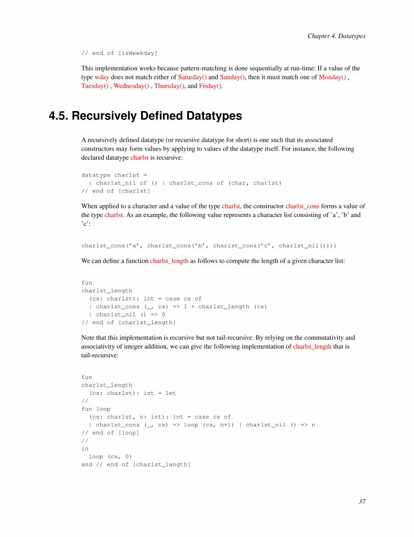
Chapter 4. Datatypes
// end of [isWeekday]
This implementation works because pattern-matching is done sequentially at run-time: If a value of thetype wday does not match either of Saturday() and Sunday(), then it must match one of Monday() ,Tuesday() , Wednesday() , Thursday(), and Friday().
4.5. Recursively Defined Datatypes
A recursively defined datatype (or recursive datatype for short) is one such that its associatedconstructors may form values by applying to values of the datatype itself. For instance, the followingdeclared datatype charlst is recursive:
datatype charlst =| charlst_nil of () | charlst_cons of (char, charlst)
// end of [charlst]
When applied to a character and a value of the type charlst, the constructor charlst_cons forms a value ofthe type charlst. As an example, the following value represents a character list consisting of ’a’, ’b’ and’c’:
charlst_cons(’a’, charlst_cons(’b’, charlst_cons(’c’, charlst_nil())))
We can define a function charlst_length as follows to compute the length of a given character list:
funcharlst_length(cs: charlst): int = case cs of| charlst_cons (_, cs) => 1 + charlst_length (cs)| charlst_nil () => 0
// end of [charlst_length]
Note that this implementation is recursive but not tail-recursive. By relying on the commutativity andassociativity of integer addition, we can give the following implementation of charlst_length that istail-recursive:
funcharlst_length(cs: charlst): int = let
//fun loop(cs: charlst, n: int): int = case cs of| charlst_cons (_, cs) => loop (cs, n+1) | charlst_nil () => n
// end of [loop]//inloop (cs, 0)
end // end of [charlst_length]
37

Chapter 4. Datatypes
Note that the naming convention I follow closely in this book (and elsewhere) mandates that only atail-recursive function be given a name indicative of its being a loop. A non-tail-recursive function is notcalled a loop because it cannot be translated directly to a loop in an imperative programming languagelike C.
4.6. Exhaustiveness of Pattern-Matching
Given a type T and a set of patterns, if for any given value of the type T there is always at least onepattern in the set such that the value matches the pattern, then pattern-matching values of the type Tagainst the set of patterns is exhaustive. Given a case-expression of the form (case exp0 of clseq), whereexp0 is assumed to be of some type T, if pattern-matching values of the type T against the guards of thematching clauses in clseq is exhaustive, then the case-expression is said to bepattern-matching-exhaustive.
The following code implements a function that finds the last character in a non-empty character list:
funcharlst_last(cs: charlst): char =
(case cs of| charlst_cons (c, charlst_nil ()) => c| charlst_cons (_, cs1) => charlst_last (cs1)
)// end of [charlst_last]
The body of charlst_last is a case-expression, which is not pattern-matching-exhaustive: If cs is bound tothe value charlst_nil(), that is, the empty character list, than none of the matching clauses in thecase-expression can be chosen. When the code is typechecked by atsopt, a warning message is issued toindicate the case-expression being non-pattern-matching-exhaustive. If the programmer wants an errormessage instead, the keyword case should be replaced with case+. If the programmer wants to suppressthe warning message, the keyword case should be replaced with case-. I myself mostly use case+ whencoding in ATS.
The function charlst_last can also be implemented as follows:
funcharlst_last(cs: charlst): char =
(case cs of| charlst_cons (c, cs1) =>(case+ cs1 of| charlst_nil () => c | charlst_cons _ => charlst_last (cs1)
) // end of [charlst_cons]) // end of [charlst_last]
38

Chapter 4. Datatypes
In this implementation, the outer case-expression is not pattern-matching-exhaustive while the inner oneis. Note that the pattern charlst_cons _ is just a shorthand for charlst_cons(_, _). In general, a pattern ofthe form C _, where C is a constructor (associated with some datatype), can be matched by any value thatis constructed by applying C to some values. For instance, the pattern charlst_nil() can also be written ascharlst_nil _.
Suppose we have a case-expression containing only one matching clause, that is, the case-expression isof the form [case exp0 of pat => exp]. Then we can also write this case-expression as a let-expression:(let val pat = exp0 in exp end). For instance, we give another implementation of the function charlst_lastas follows:
funcharlst_last(cs: charlst): char = letval charlst_cons (c, cs1) = cs in case+ cs1 of| charlst_nil () => c | charlst_cons _ => charlst_last (cs1)
end // end of [charlst_last]
When this implementation is typechecked by atsopt, a warning message is issued to indicate theval-declaration being non-pattern-matching-exhaustive. If the programmer wants an error messageinstead, the keyword val should be replaced with val+. If the programmer wants to suppress the warningmessage, the keyword val should be replaced with val-.
As values formed by the constructors charlst_nil and charlst_cons are assigned the same type charlst, it isimpossible to rely on typechecking to prevent the function charlst_last from being applied to an emptycharacter list. This is a serious limitation. With dependent types, which allow data to be described muchmore precisely, we can ensure at the level of types that a function finding the last element of a list canonly be applied to a non-empty list.
4.7. Example: Binary Search Tree
A binary search tree is a binary tree satisfying the following property: for each node in the tree, the keystored in the node is greater than or equal to every key stored in the left child of the node and less than orequal to every key stored in the right child of the node. In other words, a binary tree is a binary searchtree if a pre-order traversal encounters a sequence of keys ordered ascendingly (according to someordering on keys). In practice, binary search trees are commonly employed to represent sets and maps.
The following declaration introduces a datatype bstree for binary search trees in which the stored keysare strings:
datatype bstree =| E of () | B of (bstree, string, bstree)
// end of [bstree]
39

Chapter 4. Datatypes
It should be noted that not every value of the type bstree represents a valid binary search tree as it iscertainly possible to construct a value representing a binary tree but not a binary search tree.
The following function [bstree_inord] does a in-order traversal of a given binary tree:
funbstree_inord(t0: bstree, fwork: string -<cloref1> void
) : void =(case+ t0 of| E () => ()| B (t1, k, t2) =>{val () = bstree_inord (t1, fwork)val () = fwork (k)val () = bstree_inord (t2, fwork)
}) (* end of [bstree_inord] *)
If [t0] is a binary search tree, then the sequence of keys processed by [fwork] are ordered ascendingly.
Given a binary search tree and a key, the following function [bstree_search] checks whether the key isstored inside the tree:
funbstree_search(t0: bstree, k0: string
) : bool =(//case+ t0 of| E () => false| B (t1, k, t2) => let
val sgn = compare (k0, k)incase+ 0 of| _ when sgn < 0 => bstree_search (t1, k0)| _ when sgn > 0 => bstree_search (t2, k0)| _ (*k0 = k*) => true
end // end of [B]//) (* end of [bstree_search] *)
Note that [bstree_search] returns true if the given key is found. Otherwise, it returns false.
Given a binary search tree and a key, the following function [bstree_insert] inserts the key into the tree:
40
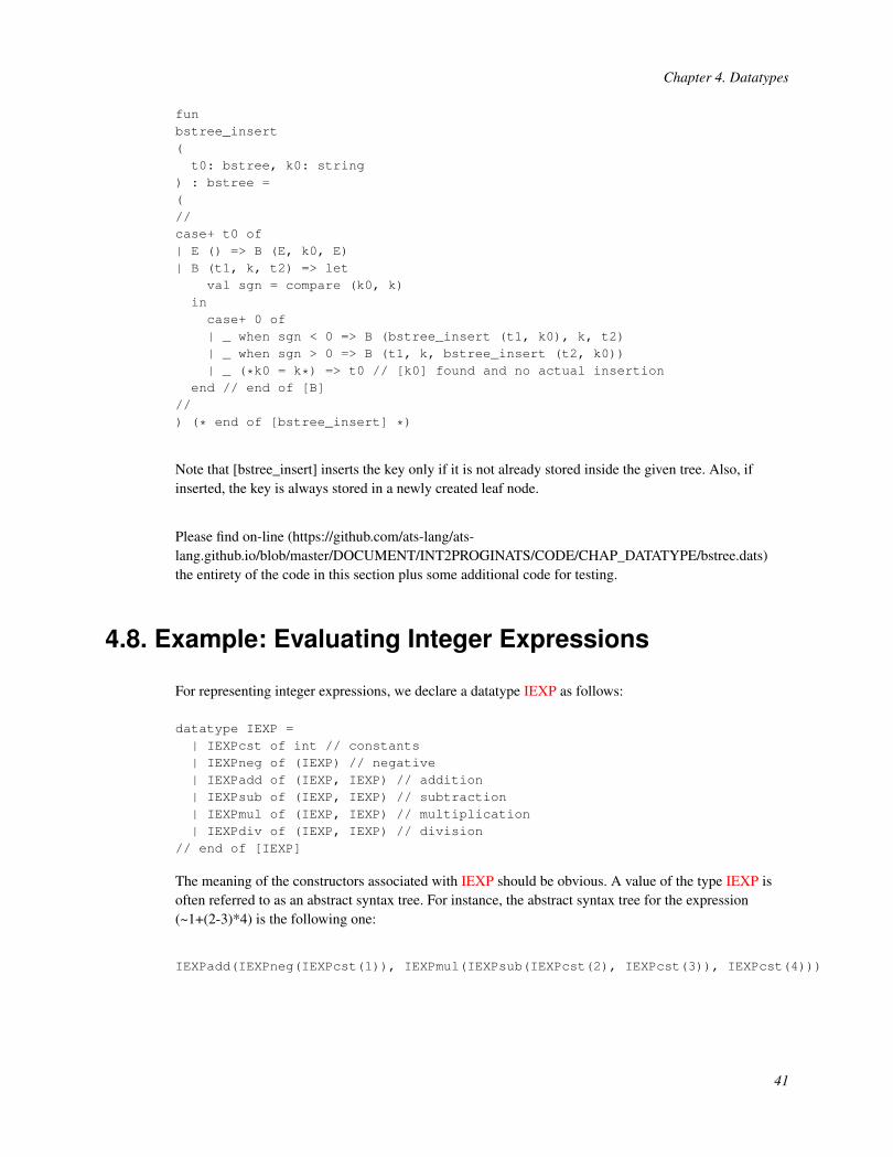
Chapter 4. Datatypes
funbstree_insert(t0: bstree, k0: string
) : bstree =(//case+ t0 of| E () => B (E, k0, E)| B (t1, k, t2) => let
val sgn = compare (k0, k)incase+ 0 of| _ when sgn < 0 => B (bstree_insert (t1, k0), k, t2)| _ when sgn > 0 => B (t1, k, bstree_insert (t2, k0))| _ (*k0 = k*) => t0 // [k0] found and no actual insertion
end // end of [B]//) (* end of [bstree_insert] *)
Note that [bstree_insert] inserts the key only if it is not already stored inside the given tree. Also, ifinserted, the key is always stored in a newly created leaf node.
Please find on-line (https://github.com/ats-lang/ats-lang.github.io/blob/master/DOCUMENT/INT2PROGINATS/CODE/CHAP_DATATYPE/bstree.dats)the entirety of the code in this section plus some additional code for testing.
4.8. Example: Evaluating Integer Expressions
For representing integer expressions, we declare a datatype IEXP as follows:
datatype IEXP =| IEXPcst of int // constants| IEXPneg of (IEXP) // negative| IEXPadd of (IEXP, IEXP) // addition| IEXPsub of (IEXP, IEXP) // subtraction| IEXPmul of (IEXP, IEXP) // multiplication| IEXPdiv of (IEXP, IEXP) // division
// end of [IEXP]
The meaning of the constructors associated with IEXP should be obvious. A value of the type IEXP isoften referred to as an abstract syntax tree. For instance, the abstract syntax tree for the expression(~1+(2-3)*4) is the following one:
IEXPadd(IEXPneg(IEXPcst(1)), IEXPmul(IEXPsub(IEXPcst(2), IEXPcst(3)), IEXPcst(4)))
41

Chapter 4. Datatypes
Translating an integer expression written in some string form into an abstract syntax tree is calledparsing, which we will not do here. The following defined function eval_iexp takes the abstract syntaxtree of an integer expression and returns an integer that is the value of the expression:
funeval_iexp(e0: IEXP): int =
(case+ e0 of| IEXPcst (n) => n| IEXPneg (e) => ~eval_iexp (e)| IEXPadd (e1, e2) => eval_iexp (e1) + eval_iexp (e2)| IEXPsub (e1, e2) => eval_iexp (e1) - eval_iexp (e2)| IEXPmul (e1, e2) => eval_iexp (e1) * eval_iexp (e2)| IEXPdiv (e1, e2) => eval_iexp (e1) / eval_iexp (e2)) (* end of [eval_iexp] *)
Suppose we also allow the construct if-then-else to be use in forming integer expressions. For instance,we may write an integer expression like (if 1+2 <= 3*4 then 5+6 else 7-8). Note that the test (1+2 <=3*4) is a boolean expression rather than an integer expression. This indicates that we also need to declarea datatype BEXP for representing boolean expressions. Furthermore, IEXP and BEXP should be definedmutually recursively as follows:
datatype IEXP =| IEXPcst of int // integer constants| IEXPneg of (IEXP) // negative| IEXPadd of (IEXP, IEXP) // addition| IEXPsub of (IEXP, IEXP) // subtraction| IEXPmul of (IEXP, IEXP) // multiplication| IEXPdiv of (IEXP, IEXP) // division| IEXPif of (BEXP(*test*), IEXP(*then*), IEXP(*else*))
// end of [IEXP]
and BEXP = // [and] for combining datatype declarations| BEXPcst of bool // boolean constants| BEXPneg of BEXP // negation| BEXPconj of (BEXP, BEXP) // conjunction| BEXPdisj of (BEXP, BEXP) // disjunction| BEXPeq of (IEXP, IEXP) // equal-to| BEXPneq of (IEXP, IEXP) // not-equal-to| BEXPlt of (IEXP, IEXP) // less-than| BEXPlte of (IEXP, IEXP) // less-than-equal-to| BEXPgt of (IEXP, IEXP) // greater-than| BEXPgte of (IEXP, IEXP) // greater-than-equal-to
// end of [BEXP]
Evidently, we also need to evaluate boolean expressions when evaluating integer expressions. Thefollowing two functions eval_iexp and eval_bexp for evaluating integer and boolean expressions,respectively, are defined mutually recursively as can be expected:
42

Chapter 4. Datatypes
funeval_iexp(e0: IEXP
) : int = (//case+ e0 of| IEXPcst n => n| IEXPneg (e) => ~eval_iexp (e)| IEXPadd (e1, e2) => eval_iexp (e1) + eval_iexp (e2)| IEXPsub (e1, e2) => eval_iexp (e1) - eval_iexp (e2)| IEXPmul (e1, e2) => eval_iexp (e1) * eval_iexp (e2)| IEXPdiv (e1, e2) => eval_iexp (e1) / eval_iexp (e1)| IEXPif(e_test, e_then, e_else
) =>(eval_iexp (if eval_bexp (e_test) then e_then else e_else)
) // end of [IEXPif]//) (* end of [eval_iexp] *)
andeval_bexp(e0: BEXP
) : bool = (//case+ e0 of| BEXPcst b => b| BEXPneg (e) => ~eval_bexp (e)| BEXPconj (e1, e2) =>
if eval_bexp (e1) then eval_bexp (e2) else false| BEXPdisj (e1, e2) =>
if eval_bexp (e1) then true else eval_bexp (e2)| BEXPeq (e1, e2) => eval_iexp (e1) = eval_iexp (e2)| BEXPneq (e1, e2) => eval_iexp (e1) != eval_iexp (e2)| BEXPlt (e1, e2) => eval_iexp (e1) < eval_iexp (e2)| BEXPlte (e1, e2) => eval_iexp (e1) <= eval_iexp (e2)| BEXPgt (e1, e2) => eval_iexp (e1) > eval_iexp (e2)| BEXPgte (e1, e2) => eval_iexp (e1) >= eval_iexp (e2)//) (* end of [eval_bexp] *)
The integer and boolean expressions used in this example are all constant expressions containing novariables. Therefore, there is no need for an environment to evaluate them. I will present a moreadvanced example elsewhere to demonstrate how an evaluator for a simple call-by-value functionalprogramming language like the core of ATS can be implemented.
43
Chapter 4. Datatypes
Please find on-line (https://github.com/ats-lang/ats-lang.github.io/blob/master/DOCUMENT/INT2PROGINATS/CODE/CHAP_DATATYPE/intexp.dats)the entirety of the code in this section plus some additional code for testing.
44

Chapter 5. Parametric Polymorphism
Code sharing is of paramount importance in programming. In a typed programming language, we oftenencounter a situation where the same functionality is needed for values of different types. For instance,we may need to compute the length of a list while the elements in the list can be characters, integers,strings, etc. Evidently, we want to avoid implementing a list-length function for each element type as itwould probably be the worst form of code duplication. We want to implement one single function thatcan be applied to any list to compute the length of the list. This list-length function parameterizes overthe element type of a given list, and it behaves uniformly regardless what the element type is. This is aform of code sharing that is often referred to as parametric polymorphism, which should be distinguishedfrom other forms of polymorphism such as inheritance polymorphism in object-oriented programming.
The code employed for illustration in this chapter plus some additional code for testing is availableon-line (https://github.com/ats-lang/ats-lang.github.io/blob/master/DOCUMENT/INT2PROGINATS/CODE/CHAP_POLYMORPH).
5.1. Function Templates
A function template is a code template that implements a function. In the following code, two functionsare defined to swap values:
//typedef charint = (char, int)typedef intchar = (int, char)//fun swap_char_int (xy: charint): intchar = (xy.1, xy.0)fun swap_int_char (xy: intchar): charint = (xy.1, xy.0)//
If types are ignored, the bodies of swap_char_int and swap_int_char are identical. In order to avoid thiskind of code duplication, we can first implement a function template swap as follows and then implementswap_char_int and swap_int_char based on swap:
//fun{a,b:t@ype} swap (xy: (a, b)): (b, a) = (xy.1, xy.0)//fun swap_char_int (xy: charint): intchar = swap<char,int> (xy)fun swap_int_char (xy: intchar): charint = swap<int,char> (xy)//
It should be noted that a function template is not a first-class value in ATS: There is no expression forrepresenting a function template. The syntax {a,b:t@ype} following the keyword fun represents templateparameters or arguments. The unusual symbol t@ype is a sort for static terms representing types of
45

Chapter 5. Parametric Polymorphism
unspecified size, where the size of a type is the number of bytes needed for representing a value of thetype (under the assumption that all of the values of the type have the same size). There is another sorttype in ATS, which is for static terms representing types of size equal to one word exactly, that is, 4 byteson a 32-bit machine or 8 bytes on a 64-bit machine. The syntax swap<char,int>, where no space isallowed between swap and < , stands for an instance of the function template swap in which theparameters a and b are replaced with char and int, respectively. The syntax swap<int,char> is interpretedsimilarly.
A different style of implementation of swap is given as follows:
fun{a:t@ype}{b:t@ype} swap2 (xy: (a, b)): (b, a) = (xy.1, xy.0)
where the template parameters are given sequentially (instead of simultaneously). The following codeshows how swap2 can be instantiated to form instances:
fun swap_char_int (xy: charint): intchar = swap2<char><int> (xy)fun swap_int_char (xy: intchar): charint = swap2<int><char> (xy)
Note that >< is a special symbol (of the name GTLT) and no space is allowed between > and <.
As another example, a higher-order function template for composing (closure) functions is given asfollows:
//typedefcfun (t1:t@ype, t2:t@ype) = t1 -<cloref1> t2//fun{a,b,c:t@ype} compose (f: cfun (a, b), g: cfun (b, c)
) :<cloref1> cfun (a, c) = lam x => g(f(x))//val inc_by_1 = lam (x:int): int =<cloref> x+1val mul_by_2 = lam (x:int): int =<cloref> x*2//val f_2x_1 = compose<int,int,int> (mul_by_2, inc_by_1)val f_2x_2 = compose<int,int,int> (inc_by_1, mul_by_2)//
It should be clear that the value f_2x_1 represents the function that multiplies its integer argument by 2and then adds 1 to the result. Similarly, the value f_2x_2 represents the function that adds 1 to its integerargument and then multiplies the result by 2.
In ATS, function templates are typechecked but not compiled to code in C. Instead, they are compiled toan intermediate form. Only instances of function templates are compiled to code in C. Suppose we havea function template foo taking one type parameter and two instances foo<T1> and foo<T2> are used in aprogram for some types T1 and T2. In general, one function in C is generated for each instance of foo
46

Chapter 5. Parametric Polymorphism
when the program is compiled. However, if T1 and T2 have the same name, then the two instances mayshare one function in C.
Please note that I may simply use the name function to refer to a function template from now on if noconfusion is expected.
5.2. Polymorphic Functions
A polymorphic function is rather similar to a function template. However, the former is a first-class valuein ATS while the latter is not. As an example, the following defined function swap_boxed ispolymorphic:
fun swap_boxed{a,b:type} (xy: (a, b)): (b, a) = (xy.1, xy.0)
The type variables a and b are often referred as static arguments while xy is a dynamic argument. Forexample, the following code makes use of the polymorphic function swap_boxed:
val AB = (box("A"), box("B"))val BA1 = swap_boxed{boxstr,boxstr} (AB)val BA2 = swap_boxed (AB) // omitting type arguments may be fine
where the type boxstr is an explicitly boxed version of string that is defined as boxed(string). Internally,there is really no difference between string and boxed(string). If swap_boxed is called on a pair of thetype (T1, T2) for some types T1 and T2, both T1 and T2 are required to be boxed. Otherwise, atype-error is reported. For example, calling swap_boxed on (0, 1) yields a type-error as the type int is notboxed. One may be attempted to form a boxed integer like box(0), but doing so leads to a type-error asthere is no assumption made about the size of an integer value of the type int in ATS.
When calling a polymorphic function, we often omit passing static arguments explicitly and expect themto be synthesized by the compiler. However, there are also occasions, which are not uncommon, wherestatic arguments need to be supplied explicitly as either they cannot be successfully synthesized or whatis synthesized is not exactly what is expected by the programmer.
It is also possible to pass static arguments sequentially as is shown in the following style ofimplementation of a polymorphic function:
//fun swap2_boxed{a:type}{b:type} (xy: (a, b)): (b, a) = (xy.1, xy.0)//val AB = (box("A"), box("B"))val BA1 = swap2_boxed (AB) // both static arguments to be synthesizedval BA2 = swap2_boxed{...} (AB) // both static arguments to be synthesizedval BA3 = swap2_boxed{..}{boxstr} (AB) // 1st static argument to be synthesizedval BA4 = swap2_boxed{boxstr}{..} (AB) // 2nd static argument to be synthesizedval BA5 = swap2_boxed{..}{..} (AB) // both static arguments to be synthesized
47

Chapter 5. Parametric Polymorphism
val BA6 = swap2_boxed{boxstr}{boxstr} (AB) // both static arguments are provided//
The special syntax {..} indicates to the typechecker that the static argument (or arguments) involved inthe current application should be synthesized while the special syntax {...} means that the rest of staticarguments should all be synthesized.
I have seen two kinds of errors involving polymorphic functions that are extremely common in practice.
• The first kind is depicted in the following example:
fun swap_boxed{a,b:t@ype} (xy: (a, b)): (b, a) = (xy.1, xy.0)
Notice that the sort for type variables a and b is t@ype (instead of type). While this example can passtypechecking, its compilation results in a compile-time error that may seem mysterious to manyprogrammers. The simple reason for this error is that the compiler cannot figure out the size of a and bwhen trying to generate code in C as the sort t@ype is for types of unspecified size.
• The second kind is depicted in the following example:
fun{a,b:type} swap_boxed (xy: (a, b)): (b, a) = (xy.1, xy.0)
Strictly speaking, there is really no error in this case. If defined as such, swap_boxed is a functiontemplate instead of a polymorphic function. However, such a function template is severely restricted asit cannot be instantiated with types that are not boxed. While this could be intended, it is very unlikely.
Given the potential confusion, why do we need both function templates and polymorphic functions? Atthis stage, it is certainly plausible that we program only with function templates and make no use ofpolymorphic functions. However, polymorphic functions simply become indispensible in the presencedependent types. There will actually be numerous occasions where we encounter polymorphic functiontemplates, that is, templates for polymorphic functions.
5.3. Polymorphic Datatypes
Code sharing also applies to datatype declarations. For instance, a commonly used polymorphic datatypelist0 is declared as follows:
datatypelist0 (a:t@ype) =| list0_nil (a) of () | list0_cons (a) of (a, list0 a)
// end of [list0]
More precisely, list0 is a type constructor. Given a type T, we can form a type list0(T) for lists consistingof elements of the type T. For instance, list0(char) is for character lists, list0(int) for integer lists,list0(list0(int)) for lists whose elements are themselves integer lists, etc. To a great extent, the need forfunction templates or polymorphic functions largely stems from the availability of polymorphicdatatypes. As an example, a function template list0_length is implemented as follows for computing thelength of any given list:
48

Chapter 5. Parametric Polymorphism
fun{a:t@ype}list0_length(xs: list0 a): int =
(case+ xs of| list0_cons (_, xs) => 1 + list0_length<a> (xs) | list0_nil () => 0
) (* end of [list0_length] *)
When applying list0_length to a list xs, we can in general write list0_length(xs), expecting thetypechecker to synthesize a proper type parameter for list0_length. We may also writelist0_length<T>(xs) if the elements of xs are of the type T. The latter style, though a bit more verbose, islikely to yield more informative messages in case type-errors occur.
Another commonly used polymorphic datatype option0 is declared as follows:
datatypeoption0 (a:t@ype) =| option0_none (a) of () | option0_some (a) of a
// end of [option0]
A typical use of option0 is to perform some kind of error-handling. Suppose that we are to implement afunction doing integer division and we want to make sure that the function returns even if it is called in acase where the divisor equals 0. This can be done as follows:
fun divopt(x: int, y: int
) : option0 (int) =if y != 0 then option0_some{int}(x/y) else option0_none((*void*))
// end of [divopt]
By inspecting what divopt returns, we can tell whether integer division has been done normally or anerror of divsion-by-zero has occurred. A realistic use of option0 is shown in the followingimplementation of list0_last:
fun{a:t@ype} list0_last(xs: list0 a
) : option0 (a) = let//fun loop(x: a, xs: list0 a): a =
(case+ xs of| list0_nil () => x | list0_cons (x, xs) => loop (x, xs)
) (* end of [loop] *)//in
49

Chapter 5. Parametric Polymorphism
case+ xs of| list0_nil () => option0_none((*void*))| list0_cons (x, xs) => option0_some{a}(loop (x, xs))
end // end of [list0_last]
When applied to a list, list0_last returns an optional value. If the value matches the patternoption0_none(), then the list is empty. Otherwise, the value is formed by applying option0_some to thelast element of the given list.
5.4. Example: Function Templates on Lists
In functional programming, lists are ubiquitous. We implement as follows some commonly used functiontemplates on lists. It should be noted that these templates are all available in some library of ATS, wherethey may be implemented in a significantly more efficient manner due to the use of certain programmingfeatures (such as linear datatypes) that have not been covered so far.
Please find the entire code in this section plus some additional code for testing on-line(https://github.com/ats-lang/ats-lang.github.io/blob/master/DOCUMENT/INT2PROGINATS/CODE/CHAP_POLYMORPH/listfuns.dats).
5.4.1. Appending: list0_append
Given two lists xs and ys of the type list0(T) for some type T, list0_append(xs, ys) returns a list that is theconcatenation of xs and ys:
fun{a:t@ype} list0_append(xs: list0 a
, ys: list0 a) : list0 a =(case+ xs of| list0_cons (x, xs) =>
list0_cons{a}(x, list0_append<a> (xs, ys))| list0_nil ((*void*)) => ys) (* end of [list0_append] *)
Clearly, this implementation of list0_append is not tail-recursive.
50

Chapter 5. Parametric Polymorphism
5.4.2. Reverse-Appending: list0_reverse_append
Given two lists xs and ys of the type list0(T) for some type T, list0_reverse_append(xs, ys) returns a listthat is the concatenation of the reverse of xs and ys:
fun{a:t@ype} list0_reverse_append(xs: list0 a, ys: list0 a
) : list0 a =(case+ xs of| list0_cons (x, xs) =>
list0_reverse_append<a> (xs, list0_cons{a}(x, ys))| list0_nil () => ys) (* end of [list0_reverse_append] *)
Clearly, this implementation of list0_reverse_append is tail-recursive.
5.4.3. Reversing: list0_reverse
Given a list xs, list0_reverse(xs) returns the reverse of xs:
fun{a:t@ype}list0_reverse(xs: list0 a): list0 a = list0_reverse_append<a> (xs, list0_nil)
// end of [list0_reverse]
5.4.4. Mapping: list0_map
Given a list xs of the type list0(T1) for some type T1 and a closure function f of the type T1 -<cloref1>T2 for some type T2, list0_map(xs, f) returns a list ys of the type list0(T2):
fun{a:t@ype}{b:t@ype}list0_map(xs: list0 a, f: a -<cloref1> b
) : list0 b =(case+ xs of| list0_cons (x, xs) =>
list0_cons{b}(f x, list0_map<a><b> (xs, f))
51

Chapter 5. Parametric Polymorphism
| list0_nil ((*void*)) => list0_nil ()) (* end of [list0_map] *)
The length of ys equals that of xs and each element y in ys equals f(x), where x is the correspondingelement in xs. Clearly, this implementation of list0_map is not tail-recursive.
5.4.5. Left-Folding: list0_foldleft
Given xs, ini and f, list0_foldleft(ini, xs, f) computes the value of the expression f(... f(f(ini, xs[0]), xs[1])..., xs[n-1]), where n is the length of xs and xs[i] refers to element i in xs for each i < n. The followingimplementation of list0_foldleft is tail-recursive:
fun{a:t@ype}{b:t@ype}list0_foldleft(ini: a, xs: list0 (b), f: (a, b) -> a
) : a =(case+ xs of| list0_cons
(x, xs) => list0_foldleft<a><b> (f (ini, x), xs, f)| list0_nil ((*void*)) => ini
)
5.4.6. Right-Folding: list0_foldright
Given xs, res and f, list0_foldright(xs, res, f) computes the value of the expression f(xs[0], f(xs[1], f(...f(xs[n-1], res) ...))), where n is the length of xs and xs[i] refers to element i in xs for each i < n. Thefollowing implementation of list0_foldright is not tail-recursive:
fun{a:t@ype}{b:t@ype}list0_foldright(xs: list0 (a), res: b, f: (a, b) -> b
) : b =(case+ xs of| list0_cons
(x, xs) => f (x, list0_foldright<a><b> (xs, res, f))| list0_nil ((*void*)) => res
)
52

Chapter 5. Parametric Polymorphism
5.4.7. Zipping: list0_zip
Given two lists xs and ys of the types list0(T1) and list0(T2) for some types T1 and T2, respectively,list0_zip(xs, ys) returns a list zs of the type list0(@(T1, T2)):
fun{a,b:t@ype} list0_zip(xs: list0 a
, ys: list0 b) : list0 @(a, b) = lettypedef ab = @(a, b)
in//case+ (xs, ys) of| (list0_cons (x, xs),
list0_cons (y, ys)) =>(list0_cons{ab}((x, y), list0_zip<a,b> (xs, ys))
)| (_, _) => list0_nil ()//end // end of [list0_zip]
The length of zs is the minimum of the lengths of xs and ys and each element z in zs equals @(x, y),where x and y are the corresponding elements in xs and ys, respectively. Clearly, this implementation oflist0_zip is not tail-recursive.
5.4.8. Zipping with: list0_zipwith
Given two lists xs and ys of the types list0(T1) and list0(T2) for some types T1 and T2, respectively, anda closure function f of the type (T1, T2) -<cloref1> T3 for some type T3, list0_zipwith(xs, ys, f) returns alist zs of the type list0(T3):
fun{a,b:t@ype}{c:t@ype}list0_zipwith(xs: list0 a
, ys: list0 b, f: (a, b) -<cloref1> c) : list0 c =(case+ (xs, ys) of
53

Chapter 5. Parametric Polymorphism
| (list0_cons (x, xs),list0_cons (y, ys)) =>
(list0_cons{c}(f (x, y), list0_zipwith<a,b><c> (xs, ys, f))
)| (_, _) => list0_nil ()) (* end of [list0_zipwith] *)
The length of zs is the minimum of the lengths of xs and ys and each element z in zs is f(x, y), where xand y are the corresponding elements in xs and ys, respectively. Clearly, this implementation oflist0_zipwith is not tail-recursive. Note that list0_zipwith behaves exactly like list0_zip if its thirdargument f is replaced with lam (x, y) => @(x, y). This function template is also named list0_map2 forthe obvious reason.
5.5. Example: Mergesort on Lists
Mergesort is a simple sorting algorithm that is guaranteed to be log-linear. It is stable in the sense that theorder of two equal elements always stay the same after sorting. I give as follows a typical functional styleof implementation of mergesort on lists.
First, let us introduce abbreviations for the list constructors list0_nil and list0_cons:
#define :: list0_cons // writing [::] for list0_cons#define cons0 list0_cons // writing [cons0] for list0_cons#define nil0 list0_nil // writing [nil0] for list0_nil
Note that the operator :: is already given the infix status. For instance, the list consisting of the first 5natural numbers can be constructed as follows:
cons0(0, cons0(1, 2 :: 3 :: 4 :: nil0((*void*))))
In practice, there is of course no point in mixing cons0 with ::.
We next implement a function template merge to merge two given ordered lists into a single ordered one:
//typedeflte (a:t@ype) = (a, a) -> bool//fun{a:t@ype} merge (xs: list0 a, ys: list0 a, lte: lte a
) : list0 a =(
54

Chapter 5. Parametric Polymorphism
case+ xs of| cons0 (x, xs1) => (case+ ys of| cons0 (y, ys1) =>
if x \lte y thencons0{a}(x, merge<a> (xs1, ys, lte))
elsecons0{a}(y, merge<a> (xs, ys1, lte))
// end of [if]| nil0 () => xs) // end of [cons0]
| nil0 () => ys) (* end of [merge] *)//
For instance, suppose that the two given lists are (1, 3, 4, 8) and (2, 5, 6, 7, 9), and the comparisonfunction (the third argument of merge) is the standard less-than-or-equal-to function on integers. Thenthe list returned by merge is (1, 2, 3, 4, 5, 6, 7, 8, 9). The syntax \lte means that the particular occurrenceof lte following the backslash symbol (\) is given the infix status, and thus the expression x \lte y meansthe same as lte(x, y).
The following function template mergesort implements the standard mergesort algorithm:
fun{a:t@ype} mergesort(xs: list0 a, lte: lte a
) : list0 a = let//val n = list0_length<a> (xs)//fun msort(xs: list0 a, n: int, lte: lte a
) : list0 a =if n >= 2 then split (xs, n, lte, n/2, nil0) else xs
//and split(xs: list0 a, n: int, lte: lte a, i: int, xsf: list0 a
) : list0 a =if i > 0 then letval-cons0 (x, xs) = xs
insplit (xs, n, lte, i-1, cons0{a}(x, xsf))
end else letval xsf = list0_reverse<a> (xsf) // make sorting stable!val xsf = msort (xsf, n/2, lte) and xs = msort (xs, n-n/2, lte)
inmerge<a> (xsf, xs, lte)
end // end of [if]
55

Chapter 5. Parametric Polymorphism
//inmsort (xs, n, lte)
end // end of [mergesort]
Suppose we want to sort the list (8, 3, 4, 1, 2, 7, 6, 5, 9); we first divide it into two lists: (8, 3, 4, 1) and (2,7, 6, 5, 9); by performing mergesort on each of them, we obtain two ordered lists: (1, 3, 4, 8) and (2, 5, 6,7, 9); by merging these two ordered list, we obtain the ordered list (1, 2, 3, 4, 5, 6, 7, 8, 9), which is apermutation of the originally given list (8, 3, 4, 1, 2, 7, 6, 5, 9).
Note that the function template merge is not tail-recursive as the call to merge in its body is not atail-call. This can be a serious problem in practice: It is almost certain that a stack overflow is to occur ifthe above implementation of mergesort is employed to sort a list that is very long (e.g., containing1,000,000 elements or more). I will later give a tail-recursive implementation of the merge function inATS that makes use of linear types.
Please find the entire code in this section plus some additional code for testing on-line(https://github.com/ats-lang/ats-lang.github.io/blob/master/DOCUMENT/INT2PROGINATS/CODE/CHAP_POLYMORPH/mergesort.dats).
56
II. Support for PracticalProgramming

Chapter 6. Effectful Programming Features
Effectful programming features are those that can generate effects at run-time. But what is really aneffect? The answer to this question is rather complex as it depends on the model of evaluation. I willgradually introduce various kinds of effects in this book. In sequential programming, that is, constructingprograms to be evaluated sequentially (in contrast to concurrently), an expression is effectless if thereexists a value such that the expression and the value cannot be distinguished as far as evaluation isconcerned. For instance, the expression 1+2 is effectless as it cannot be distinguished from the value 3.An effectless expression is also said to be pure. On the other hand, an effectful expression is one that canbe distinguished from any given values. For instance, the expression print("Hello") is effectful as itsevaluation results in an observable behavior that distinguishes the expression from any values. In thiscase, print("Hello") is said to certain I/O effect. If the evaluation of an expression never terminates, thenthe expression is also effectul. For instance, let us define a function loop as follows:
fun loop (): void = loop ()
Then the expression loop() can be distinguished from any values in the following context:
let val _ = [] in print ("Terminated") end
If the hole [] in the context is replaced with loop(), then the evaluation of the resulting expressioncontinues forever. If the hole [] is replaced with any value, then the evaluation leads to the string"Terminated" being printed out. The expression loop is said to contain non-termination effect.
I will cover programming features related to exceptional control-flow, persistent memory storage andsimple I/O in this chapter, which are all of common use in practical programming.
The code employed for illustration in this chapter plus some additional code for testing is availableon-line (https://github.com/ats-lang/ats-lang.github.io/blob/master/DOCUMENT/INT2PROGINATS/CODE/CHAP_EFFECTFUL/).
6.1. Exceptions
The exception mechanism provides an efficient means for reporting a special condition encounteredduring program evaluation. Often such a special condition indicates an error, but it is not uncommon toemploy exceptions to address issues that are not related to errors.
The type exn is predefined in ATS. One may think of exn as an extensible datatype for which newconstructors can always be declared. For instance, two exception constructors are declared as follows:
exception FatalError0 of ()exception FatalError1 of (string)
58
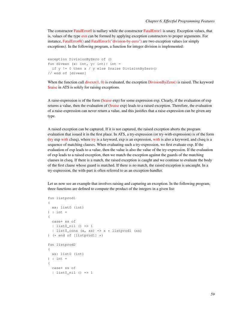
Chapter 6. Effectful Programming Features
The constructor FatalError0 is nullary while the constructor FatalError1 is unary. Exception values, thatis, values of the type exn can be formed by applying exception constructors to proper arguments. Forinstance, FatalError0() and FatalError1("division-by-zero") are two exception values (or simplyexceptions). In the following program, a function for integer division is implemented:
exception DivisionByZero of ()fun divexn (x: int, y: int): int =if y != 0 then x / y else $raise DivisionByZero()
// end of [divexn]
When the function call divexn(1, 0) is evaluated, the exception DivisionByZero() is raised. The keyword$raise in ATS is solely for raising exceptions.
A raise-expression is of the form ($raise exp) for some expression exp. Clearly, if the evaluation of expreturns a value, then the evaluation of ($raise exp) leads to a raised exception. Therefore, the evaluationof a raise-expression can never return a value, and this justifies that a raise-expression can be given anytype.
A raised exception can be captured. If it is not captured, the raised exception aborts the programevaluation that issued it in the first place. In ATS, a try-expression (or try-with-expression) is of the form(try exp with clseq), where try is a keyword, exp is an expression, with is also a keyword, and clseq is asequence of matching clauses. When evaluating such a try-expression, we first evaluate exp. If theevaluation of exp leads to a value, then the value is also the value of the try-expression. If the evaluationof exp leads to a raised exception, then we match the exception against the guards of the matchingclauses in clseq. If there is a match, the raised exception is caught and we continue to evaluate the bodyof the first clause whose guard is matched. If there is no match, the raised exception is uncaught. In atry-expression, the with-part is often referred to as an exception-handler.
Let us now see an example that involves raising and capturing an exception. In the following program,three functions are defined to compute the product of the integers in a given list:
fun listprod1(xs: list0 (int)
) : int =(case+ xs of| list0_nil () => 1| list0_cons (x, xs) => x * listprod1 (xs)
) (* end of [listprod1] *)
fun listprod2(xs: list0 (int)
) : int =(case+ xs of| list0_nil () => 1
59

Chapter 6. Effectful Programming Features
| list0_cons (x, xs) =>if x = 0 then 0 else x * listprod2 (xs)
// end of [list0_cons]) (* end of [listprod2] *)
fun listprod3(xs: list0 (int)
) : int = letexception ZERO of ()fun aux (xs: list0 (int)): int =case+ xs of| list0_cons (x, xs) =>
if x = 0 then $raise ZERO() else x * aux (xs)| list0_nil () => 1
// end of [aux]intry aux (xs) with ~ZERO () => 0
end // end of [listprod3]
While these functions can all be defined tail-recursively, they are not so as to make a point that should beclear shortly. Undoubtedly, we all know the following simple fact:
• If the integer 0 occurs in a given list, then the product of the integers in the list is 0 regardless whatother integers are.
The function listprod1 is defined in a standard manner, and it does not make any use of the stated fact.The function listprod2 is defined in a manner that makes only partial use of the stated fact. To see thereason, let us evaluate a call to listprod2 on [1, 2, 3, 0, 4, 5, 6], which denotes a list consisting of the 7mentioned integers. The evaluation of this call eventually leads to the evaluation of1*(2*(3*(listprod([0,4,5,6])))), which then leads to 1*(2*(3*0)), and then to 1*(2*0), and then to 1*0,and finally to 0. However, what we really want is for the evaluation to return 0 immediately once theinteger 0 is encountered in the list, and this is accomplished by the function listprod3. When evaluating acall to listprod3 on [1, 2, 3, 0, 4, 5, 6], we eventually reach the evaluation of the following expression:
try 1*(2*(3*(aux([0,4,5,6])))) with ~ZERO() => 0
Evaluating aux([0,4,5,6]) leads to the exception ZERO() being raised, and this raised exception is caughtand 0 is returned as the value of the call to listprod3. Note that the pattern guard of the matching clausefollowing the keyword with is ~ZERO(). I will explain the need for the tilde symbol ~ elsewhere. Fornow, it suffices to say that exn is a linear type and each exception value is a linear value, which must beconsumed or re-raised. The tilde symbol ~ indicates that the value matching the pattern following ~ isconsumed (and the memory for holding the value is freed).
Exceptions are not a programming feature that is easy to master, and misusing exceptions is abundant inpractice. So please be patient when learning the feature and be cautious when using it.
60

Chapter 6. Effectful Programming Features
6.2. Example: Testing for Braun Trees
Braun trees are special binary trees that can be defined inductively as follows:
• If a binary tree is empty, then it is a Braun tree.
• If both children of a binary tree are Braun trees and the size of the left child minus the size of the rightchild equals 0 or 1, then the binary tree is a Braun tree.
Given a natural number n, there is exactly one Braun tree of size n. It is straightforward to prove thatBraun trees are balanced.
A polymorphic datatype is declared as follows for representing binary trees:
datatype tree (a:t@ype) =| tree_nil of ((*void*))| tree_cons of (a, tree(a)(*left*), tree(a)(*right*))
// end of [tree] // end of [datatype]
The following defined function brauntest0 tests whether a given binary tree is a Braun tree:
fun{a:t@ype} size (t: tree a): int = case+ t of| tree_nil () => 0| tree_cons (_, tl, tr) => 1 + size(tl) + size(tr)
// end of [size]
fun{a:t@ype} brauntest0(t: tree a): bool =
(case+ t of| tree_nil () => true| tree_cons (_, tl, tr) => let
val cond1 = brauntest0(tl) andalso brauntest0(tr)inif cond1 then letval df = size(tl) - size(tr) in (df = 0) orelse (df = 1)
end else falseend // end of [tree_cons]
) (* end of [brauntest0] *)
The implementation of brauntest0 follows the definition of Braun trees closely. If applied to binary treesof size n, the time-complexity of the function size is O(n) and the time-complexity of the functionbrauntest0 is O(n(log(n))).
In the following program, the defined function brauntest1 also tests whether a given binary tree is aBraun tree:
61

Chapter 6. Effectful Programming Features
fun{a:t@ype} brauntest1(t: tree a): bool = letexception Negative of ()fun aux (t: tree a): int =(case+ t of| tree_nil () => 0| tree_cons (_, tl, tr) => let
val szl = aux (tl) and szr = aux (tr)val df = szl - szr
inif df = 0 orelse df = 1 then 1+szl+szr else $raise Negative()
end // end of [tree_cons]) (* end of [aux] *)
intry letval _ = aux (t)
intrue // [t] is a Braun tree
end with~Negative() => false // [t] is not a Braun tree
// end of [try]end // end of [brauntest1]
Clearly, a binary tree cannot be a Braun tree if one of its subtrees, proper or improper, is not a Braun tree.The auxiliary function aux is defined to return the size of a binary tree if the tree is a Braun tree or raisean exception otherwise. When the evaluation of the try-expression in the body of brauntest1 starts, thecall to aux on a binary tree t is first evaluated. If the evaluation of this call returns, then t is a Braun treeand the boolean value true is returned as the value of the try-expression. Otherwise, the exceptionNegative() is raised and then caught, and the boolean value false is returned as the value of thetry-expression. The time complexity of brauntest1 is the same as that of aux, which is O(n).
The use of the exception mechanism in the implementation of brauntest1 is a convincing one because therange between the point where an exception is raised and the point where the raised exception is capturedcan span many function calls. If this range is short (e.g., spanning only one function call) in a case, thenthe programmer should probably investigate whether it is a sensible use of the exception mechanism. Forinstance, the use of exception in the following example may seem interesting but it actually leads to veryinefficient code:
fun{a:t@ype} list0_length(xs: list0 (a)): int =try 1 + list0_length (xs.tail()) with ~ListSubscriptExn() => 0
// end of [list0_length]
Therefore, making use of exceptions in this style should be avoided.
62

Chapter 6. Effectful Programming Features
Please find the entirety of the code in this section plus some additional code for testing on-line(https://github.com/ats-lang/ats-lang.github.io/blob/master/DOCUMENT/INT2PROGINATS/CODE/CHAP_EFFECTFUL/brauntest.dats).
6.3. References
A reference is just a singleton array, that is, an array containing one element. Given a type T, a referencefor storing a value of the type T is given the type ref(T). The following simple program makes use of allthe essential functionalities on references:
val intr = ref<int> (0) // create a ref and init. it with 0val () = !intr := !intr + 1 // increase the integer at [intr] by 1
The first line creates a reference for storing an integer and initializes it with the value 0 and then names itintr. Note that this style of reference creation cannot be separated from its initialization. The second lineupdates the reference intr with its current value plus 1. In general, given a reference r of type ref(T) forsome T, the expression !r means to fetch the value stored at r, which is of the type T. However, !r can alsobe used as a left-value. For instance, the assignment (!r := exp) means to evaluate exp into a value andthen store the value into r. Therefore, the value stored in intr is 1 after the second line in the aboveprogram is evaluated.
Various functions and function templates on references are declared in the file reference.sats(https://github.com/ats-lang/ats-lang.github.io/blob/master/DOCUMENT/ATS-Postiats/prelude/SATS/reference.sats), which is automatically loaded by atsopt. In particular, it is alsopossible to read from and write to a reference by using the function templates ref_get_elt and ref_set_eltof the following interfaces, respectively:
fun{a:t@ype} ref_get_elt (r: ref a): a // !rfun{a:t@ype} ref_set_elt (r: ref a, x: a): void // !r := x
References are often misused in practice, especially, by beginners of functional programming who hadsome previous exposure to imperative programming languages such C and Java. Such programmersoften think that they can just "translate" their programs in C or Java into functional programs. Forexample, the following defined function sumup is such an example, which sums up all the integersbetween 1 and a given integer, inclusive:
fun sumup(n: int): int = letval i = ref<int> (1)val res = ref<int> (0)fun loop (): void =if !i <= n then (!res := !res + !i; !i := !i + 1; loop ())
// end of [loop]inloop (); !res
63

Chapter 6. Effectful Programming Features
end // end of [sumup]
This is a correct but poor implementation, and its style, though not the worst of its kind, is deplorable. Asreferences are allocated in heap, reading from or writing to a reference can be much moretime-consuming than reading from or writing to a register. So, this implementation of sumup is unlikelyto be time-efficient. Every call to sumup creates two references in heap and leaves them there when itreturns, and the memory allocated for such references can only be reclaimed through garbage collection(GC). So, this implementation of sumup is not memory-efficient. More importantly, a program makingheavy use of references is often difficult to reason about.
I consider references a dangerous feature in functional programming. If you want to run your programwithout GC, please do not create references in the body of a function (besides many other restrictions). Ifyou find that you are in need of references to "translate" imperative programs into functional ones, then itis most likely that you are lost and you have not learned well to program in a functional style yet.
6.4. Example: A Counter Implementation
Let us see as follows the implementation of a counter-like object in the style of object-orientedprogramming (OOP). The type counter for counters is defined as follows:
typedefcounter = ’{get= () -<cloref1> int
, inc= () -<cloref1> void, reset= () -<cloref1> void} // end of [counter]
The three fields of counter are closure functions that correspond to methods associated with an object:getting the count of the counter, increasing the count of the counter by 1 and resetting the count of thecounter to 0. The following defined function newCounter is for creating a counter object (represented asa boxed record of closure functions):
fun newCounter(// argumentless) : counter = letval count = ref<int> (0)
in ’{get= lam () => !count
, inc= lam () => !count := !count + 1, reset= lam () => !count := 0} end // end of [newCounter]
The state of each created counter object is stored in a reference, which can only be accessed by the threeclosure functions in the record that represents the object. This is often referred to as state encapsulationin OOP.
64

Chapter 6. Effectful Programming Features
I myself think that the above counter implementation is of rather a poor style. It is also possible to protectthe integrity of a state by simply making it abstract. I will present elsewhere another counterimplementation based on a linear abstract type (that is, abstract viewtype in ATS), where counters can becreated and then safely freed.
6.5. Arrays
I mentioned earlier that a reference is just an array of size 1. I would now like to state that an array ofsize n is just n references allocated consecutively. These references can also be called cells, and they arenumbered from 0 until n-1, inclusive.
Given an array of size n, an integer is a valid index for this array if it is a natural number strictly less thann. Otherwise, the integer is out of the bounds of the array. For an array named A, the expression A[i]means to fetch the content of the cell in A that is numbered i if i is a valid index for A. The expressionA[i] can also be used as a left value. For instance, the assignment (A[i] := exp) means to evaluate exp to avalue and then store the value into the cell in A that is numbered i if i is a valid index.
What happens if the index i in A[i] is invalid, that is, it is out of the bounds of the array A? In this case,A[i] is referred to as out-of-bounds array subscription and evaluating A[i] leads to a raised exceptionwhere the exception is ArraySubscriptExn(). One simple and reliable way to tell whether an integer is avalid index for a given array is to compare it with the size of the array at run-time. Given a type T, thetype arrszref(T) is for an array paired with its size in which elements of the type T are stored. I willloosely refer to values of the type arrszref(T) as arrays from now on. In case there is a clear need to avoidpotential confusion, I may also refer to them as array0-values.
Various functions and function templates on array0-values are declared in the file arrayref.sats(https://github.com/ats-lang/ats-lang.github.io/blob/master/DOCUMENT/ATS-Postiats/prelude/SATS/arrayref.sats), which is automatically loaded by atsopt. For instance, threefunction templates and one polymorphic function on arrays are depicted by the following interfaces:
//fun{a:t@ype} // templatearrszref_make_elt(asz: size_t, x: a): arrszref a // array creation
//// polymorphic fun://fun arrszref_get_size{a:t@ype} (A: arrszref a): size_t // size of an array
//fun{a:t@ype} // templatearrszref_get_elt_at (A: arrszref a, i: size_t): a // A[i]//fun{a:t@ype} // templatearrszref_set_elt_at (A: arrszref a, i: size_t, x: a): void // A[i] := x//
65

Chapter 6. Effectful Programming Features
As for programming with arrays that carry no size information, it is a topic to be covered after dependenttypes are introduced.
Like in C, there are many types of integer values in ATS. The type size_t is essentially for unsigned longintegers. The functions for converting between the type int and the type size_t are g0int2uint_int_sizeand g0uint2int_size_int. Given a type T and two values asz and init of the types size_t and T,respectively, arrszref_make_elt<T> (asz, init) returns an array of the type arrszref(T) such that the size ofthe array is asz and each cell in the array is initialized with the value init. Given an array A of the typearrszref(T) for some T, arrszref_get_size(A) returns the size of A, which is of the type size_t. Forconvenience, arrszref_get_size(A) can be written as A.size(). As for array access and update, thefunctions arrszref_get_elt_at and arrszref_set_elt_at can be called. For convenience, the bracket notationcan be used to call these functions.
In the following program, the function template insertion_sort implements the standard insertion sort onarrays:
fun{a:t@ype} insertion_sort(A: arrszref (a)
, cmp: (a, a) -> int) : void = letval n = g0uint2int_size_int(A.size())fun ins (x: a, i: int):<cloref1> void =if i >= 0 then(if cmp (x, A[i]) < 0then (A[i+1] := A[i]; ins (x, i-1)) else A[i+1] := x
// end of [if]) else A[0] := x // end of [if]
// end of [ins]fun loop (i: int):<cloref1> void =if i < n then (ins (A[i], i-1); loop (i+1)) else ()
// end of [loop]inloop (1)
end // end of [insertion_sort]
The comparison function cmp should return 1, -1, and 0 if its first argument is greater than, less than andequal to its second one, respectively.
Note that the entire code in this section plus some additional code for testing is available on-line(https://github.com/ats-lang/ats-lang.github.io/blob/master/DOCUMENT/INT2PROGINATS/CODE/CHAP_EFFECTFUL/insort.dats).
66

Chapter 6. Effectful Programming Features
6.6. Example: Ordering Permutations
Given a natural number n, we want to print out all the permutations consisting of integers ranging from 1to n, inclusive. In addition, we want to print them out according to the lexicographic ordering on integersequences. For instance, we want the following output to be generated when n is 3:
1, 2, 31, 3, 22, 1, 32, 3, 13, 1, 23, 2, 1
Let us first define a function as follows for printing out an array of integers:
fun print_intarray(A: arrszref (int)): void = letval asz = g0uint2int_size_int(A.size())
//// The integers are to be separated by the string [sep]//fun loop (i: int, sep: string): void =if i < asz then(if i > 0 then print sep; print A[i]; loop (i+1, sep))
// end of [if]inloop (0, ", ")
end // end of [print_intarray]
We next implement two functions lrotate and rrotate for rearranging the elements in a given integer array:
fun lrotate (A: arrszref int, i: int, j: int
) : void = letfun lshift (A: arrszref int, i: int, j: int
) : void =if i < j then (A[i] := A[i+1]; lshift (A, i+1, j))
inif i < j then letval tmp = A[i] in lshift (A, i, j); A[j] := tmp
end // end of [if]end // end of [lrotate]
fun rrotate (
67

Chapter 6. Effectful Programming Features
A: arrszref int, i: int, j: int) : void = letfun rshift (A: arrszref int, i: int, j: int
) : void =if i < j then (A[j] := A[j-1]; rshift (A, i, j-1))
inif i < j then letval tmp = A[j] in rshift (A, i, j); A[i] := tmp
end // end of [if]end // end of [rrotate]
When applied to an array and two valid indexes i and j for the array such that i is less than or equal to j,lrotate moves simultaneously the content of cell i into cell j and the content of cell k to cell k-1 for kranging from i+1 to j, inclusive. The function rrotate is similar to lrotate but shuffles elements in theopposite direction.
Given a natural number n, the following defined function permute prints out all the permutationsconsisting of integers ranging from 1 to n, inclusive while arranging the output according to thelexicographic ordering on integer sequences.
fun permute(n: int): void = let
//#define i2sz g0int2uint_int_size
//// Creating array A of size n//val A = arrszref_make_elt<int> (i2sz(n), 0)
//// Initializing A with integers from 1 to n, inclusive//val () = init(0) where{fun init (i: int): void =if i < n then (A[i] := i+1; init (i+1))
} // end of [where] // end of [val]//fun aux(i: int): void =
(if i <= nthen aux2 (i, i)else (print_intarray (A); print_newline ()
) (* end of [else] *)) (* end of [aux] *)
//and aux2(i: int, j: int): void =
(if j <= n then let
68

Chapter 6. Effectful Programming Features
val () = (rrotate (A, i-1, j-1); aux (i+1); lrotate (A, i-1, j-1)
) // end of [val]inaux2 (i, j+1)
end // end of [if]) (* end of [aux2] *)
//inaux (1)
end // end of [permute]
Note that where is a keyword, and the expression (exp where { decseq }) for some expression exp anddeclaration sequence decseq is equivalent to the let-expression of the form (let decseq in exp end). Tounderstand the behavior of the function aux, let us evaluate aux(1) while assuming that n is 4 and the 4elements of the array A are 1, 2, 3, and 4. It should be fairly straightforward to see that this evaluationleads to the evaluation of aux(2) for 4 times: the array A contains (1, 2, 3, 4) for the first time, and (2, 1,3, 4) for the second time, and (3, 1, 2, 4) for the third time, and (4, 1, 2, 3) for the fourth time. With someinductive reasoning, it should not be difficult to see that evaluating aux(1) indeed leads to all thepermutations being output according to the lexicographic ordering on integer sequences.
Please find the entire code in this section plus some additional code for testing on-line(https://github.com/ats-lang/ats-lang.github.io/blob/master/DOCUMENT/INT2PROGINATS/CODE/CHAP_EFFECTFUL/permord.dats).
6.7. Matrices
A matrix in ATS is just a two-dimensional array but it is represented by a one-dimensional array and therepresentation is of the row-major style (in contrast to the column-major style). Given a type T, the typemtrxszref(T) is for a matrix combined with its number of rows and number of columns such that eachelement stored in the matrix is of the type T. I will loosely refer to values of the type mtrxszref(T) asmatrices from now on. If there is a clear need to avoid potential confusion, I may also refer to them asmatrix0-values.
Given a matrix M of dimension m by n, the expression M[i,j] means to fetch the content of the cell in Mthat is indexed by (i, j), where i and j are natural numbers strictly less than m and n, respectively. Theexpression M[i,j] can also be used as a left value. For instance, the assignment (M[i,j] := exp) means toevaluate exp to a value and then store the value into the cell in M that is indexed by (i, j).
Various functions and function templates on matrix0-values are declared in the file matrixref.sats(https://github.com/ats-lang/ats-lang.github.io/blob/master/DOCUMENT/ATS-Postiats/prelude/SATS/matrixref.sats), which is automatically loaded by atsopt. For instance, threefunction templates and two polymorphic functions on matrices are depicted by the following interfaces:
//fun{a:t@ype}
69

Chapter 6. Effectful Programming Features
mtrxszref_make_elt // template(row: size_t, col: size_t, x: a): mtrxszref (a)
//fun mtrxszref_get_nrow{a:t@ype} (M: mtrxszref a): size_t // polyfunfun mtrxszref_get_ncol{a:t@ype} (M: mtrxszref a): size_t // polyfun//fun{a:t@ype}mtrxszref_get_elt_at // template(M: mtrxszref a, i: size_t, j: size_t): a // M[i,j]
fun{a:t@ype}mtrxszref_set_elt_at // template(M: mtrxszref a, i: size_t, j: size_t, x: a): void // M[i,j] := x
//
Given a type T and three values nrow, ncol and init of the types size_t, size_t and T, respectively,mtrxszref_make_elt<T> (row, col, init) returns a matrix of the type mtrxszref(T) such that the dimensionof the matrix is nrow by ncol and each cell in the matrix is initialized with the value init. Given a matrixM of the type mtrxszref(T) for some T, mtrxszref_get_nrow(M) and mtrxszref_get_ncol(M) return thenumber of rows and the number of columns of M, respectively, which are both of the type size_t. Forconvenience, mtrxszref_get_nrow(M) and mtrxszref_get_ncol(M) can also be written as M.nrow andM.ncol, respectively. As for matrix access and update, the function templates mtrxszref_get_elt_at andmtrxszref_set_elt_at can be called, respectively. For convenience, bracket notation can used for thesefunctions.
Let us now take a look at an example. The following defined function mtrxszref_transpose turns a givenmatrix into its transpose:
fun{a:t@ype}mtrxszref_transpose(M: mtrxszref a): void = let
//val nrow = mtrxszref_get_nrow (M)//fnx loop1(i: size_t): void =if i < nrow then loop2 (i, 0) else ()
//and loop2(i: size_t, j: size_t): void =if j < i then letval tmp = M[i,j]
inM[i,j] := M[j,i]; M[j,i] := tmp; loop2 (i, j+1)
end elseloop1 (i+1)
// end of [if]//in
70

Chapter 6. Effectful Programming Features
loop1 (0)end // end of [mtrxszref_transpose]
The matrix M is assumed to be a square, that is, its number of rows equals its number of columns. Notethat the two functions loop1 and loop2 are defined mutually tail-recursively, and the keyword fnxindicates the need to combine the bodies of loop1 and loop2 so that mutual recursive tail-calls in thesefunction bodies can be compiled into direct local jumps.
6.8. Example: Estimating the Constant Pi
I present as follows a Monte Carlo approach to estimating the constant Pi, the ratio of the circumferenceof a circle over its diameter.
Assume that we have a square of the dimension N by N, where N is a relatively large natural number(e.g., 1000), and a disk of radius 1 that is contained in the square. Let N2 stand for N*N, that is, thesquare of N. If we randomly choose a point inside the square, then the probability for the point to hit thedisk is Pi/N2.
The experiment we use to estimate the constant Pi can be described as follows. Given a natural numberK, let us randomly choose K points inside the square in K rounds. In each round, we choose exactly onepoint. If the point chosen in round k hits on the disk centered at a previously chosen point, then werecord one hit. Clearly, the expected number of hits recorded in round k is (k-1)*Pi/N2 as k-1 points havealready being chosen in the previous rounds. Therefore, in K rounds, the expected total number of hits is(K*(K-1)/2)*Pi/N2. If K is fixed to be N2, then the expected total number of hits is (N2-1)*Pi/2. It canbe proven that the total number of hits divided by N2 converges to Pi/2 (with probability 1) as Napproaches infinity.
If we implement the above experiment directly based on the given description, the time-complexity ofthe implementation is evidently proportional to N2*N2 as the time spent in round k is proportional to k,where k ranges from 1 to N2. An implementation as such is simply impractical for handling N aroundthe order 1000 (and thus N2 around the order of 1,000,000). To address the issue, we can impose a gridon the square, dividing it into N2 unit squares (of the dimension 1 by 1). We then associate with eachunit square a list of chosen points that are inside it. In each round, we first choose a point randomlyinside the original square; we next locate the unit square that contains this point; we then only search thelists associated with the unit square or any of its neighbors to count the number of hits generated by thepoint chosen in this round as this point cannot hit any disks centered at points that are not on these lists.As each unit square can have at most 8 neighbors and the average length of the list associated with eachsquare is less than 1 during the experiment, the time spent during each round is O(1), that is, bounded bya constant. Hence, the time taken by the entire experiment is O(N2).
An implementation that precisely matches the above description plus some testing code is availableon-line (https://github.com/ats-lang/ats-lang.github.io/blob/master/DOCUMENT/INT2PROGINATS/CODE/CHAP_EFFECTFUL/montecarlo.dats).
71

Chapter 6. Effectful Programming Features
6.9. Simple Input and Output
Handling I/O in ATS properly requires the availability of both dependent types and linear types, which Iwill cover elsewhere. In this section, I only present a means for allowing the programmer to accesscertain very basic I/O functionalities.
A file handle essentially associates a stream (of bytes) with a file identifier (represented as an integer). InATS, the type for file handles is FILEref. There are three standard file handles, which are listed asfollows:
• stdin_ref: standard input
• stdout_ref: standard output
• stderr_ref: standard error output
Various functions on file handles are declared in the file filebas.sats (https://github.com/ats-lang/ats-lang.github.io/blob/master/DOCUMENT/ATS-Postiats/prelude/SATS/filebas.sats), which isautomatically loaded by atsopt. For instance, the functions for opening and closing file handles have thefollowing interfaces:
fun fileref_open_exn(path: string, fm: file_mode
) : FILEref // endfun
fun fileref_close (fil: FILEref): void
Note that these two functions abort immediately whenever an error occurs. The following function is anoptional version of fileref_open_exn, and the caller needs to inspect the value returned by a call tofileref_open_opt to see if a file handle is actually obtained.
fun fileref_open_opt(path: string, fm: file_mode) : Option_vt(FILEref)
The type file_mode is for values representing file modes, which are listed as follows:
• file_mode_r: opening a file for reading and positioning the associated stream at the beginning of thefile.
• file_mode_rr: opening a file for both reading and and writing and positioning the associated stream atthe beginning of the file.
• file_mode_w: truncating a given file to zero length or creating a new one for writing and positioningthe associated stream at the beginning of the file.
• file_mode_ww: truncating a given file to zero length or creating a new one for both reading andwriting and positioning the associated stream at the beginning of the file.
72

Chapter 6. Effectful Programming Features
• file_mode_a: opening a file for writing and positioning the associated stream at the end of the file.
• file_mode_aa: opening a file for both reading and writing and positioning the associated stream at thebeginning of the file for reading and at the end for writing.
As an example, the following short program opens a file handle, outputs the string "Hello, world!" plus anewline into the stream associated with the file handle and then closes the file handle:
implementmain0 () ={val out =fileref_open_exn ("hello.txt", file_mode_w)
val () = fprint_string (out, "Hello, world!\n")val () = fileref_close (out)//} (* end of [main0] *)
After executing the program, we obtain a file of the name "hello.txt" in the current working directorycontaining the expected content. There are various fprint-functions in ATS for printing out data into thestream associated with a given file handle. Often the programmer can simply use the name fprint to referto these functions due to the support for overloading in ATS.
Another common I/O function is given the following interface:
fun fileref_get_line_string(fil: FILEref): Strptr1
The function fileref_get_line_string reads a line from the stream associated with a given file handle, andit returns a value of the type Strptr1. For the moment, I will simply say that such a value is just like astring except that it needs to be freed explicitly. As an example, the following short program echos ontothe standard output each line read from the standard input:
implementmain0 (// argumentless) = loop () where{//fun loop (): void = letval isnot = fileref_isnot_eof (stdin_ref)
in//if isnot then letval line =fileref_get_line_string (stdin_ref)
val ((*void*)) = fprintln! (stdout_ref, line)val ((*void*)) = strptr_free (line)
inloop ()
end else ((*loop exits as the end-of-file is reached*))
73

Chapter 6. Effectful Programming Features
//end (* end of [loop] *)//} (* end of [main0] *)
Note that the function strptr_free is called to free a linear string (of the type Strptr1). Often, typing theCTRL-D character can terminate the above program for echoing each line of input.
74

Chapter 7. Modularity
Generally speaking, modularity in programming means to organize programs in a modular fashion sothat they each can be constructed in a relatively isolated manner and then be combined to functioncoherently. I will introduce in this section some features in ATS that are largely designed to facilitateprogram organization.
The code employed for illustration in this chapter plus some additional code for testing is availableon-line (https://github.com/ats-lang/ats-lang.github.io/blob/master/DOCUMENT/INT2PROGINATS/CODE/CHAP_MODULARITY/).
7.1. Types as a Form of Specification
The interface for a function or value specifies a type that any implementation of the function or valueshould possess. For instance, the following code defines a function fact for computing the factorial of agiven integer:
fun fact (x: int): int = if x > 0 then x * fact (x-1) else 1
It is also possible to first declare an interface for fact as follows:
extern fun fact (x: int): int
where extern is a keyword in ATS that initiates the declaration of an interface. Alternative ways todeclare an interface for fact are given as follows:
extern fun fact : (int) -> intextern val fact : (int) -> int
If fact is declared to be a function, then it is required to be applied when occurring in code. If it isdeclared to be a value, there is no such a restriction.
A function interface can be considered as a form of specification. For instance, the above interface forfact specifies that fact is a function that takes one argument required to be an integer and returns a valueguaranteed to be an integer. What is so special about this form of specification is that it is formallyenforced in ATS through typechecking: Any well-typed implementation of fact in ATS must possess theinterface declared for it. Of course, this interface for fact is not a precise specification as there are(infinitely) many functions that can be given the same interface. This kind of imprecision can, however,be reduced or even eliminated, sometimes. After dependent types are introduced, I will present aninterface for fact such that any implementation of the interface is guaranteed to implement precisely thefactorial function as is defined by the following two equations:
• fact(0) = 1
75

Chapter 7. Modularity
• fact(n) = n * fact (n-1) for each natural number n > 0
An implementation for fact as the following one can be given at any point where the declared interfacefor fact is accessible:
implement fact (x) = if x > 0 then x * fact (x-1) else 1
The keyword implement is for initiating an implementation of a function or value whose interface isalready declared. It is fairly common to see the following style of coding, usually, by a beginning ATSprogrammer:
implement fact (x: int): int = if x > 0 then x * fact (x-1) else 1
While this implementation can pass typechecking, it is nonetheless of a poor style: The types providedby the programmer for the argument and the result of fact are redundant as they can be automaticallysynthesized by the typechecker.
As an example of an interface for a value, fact10 is declared as follows to be a value of the type int:
extern val fact10 : int
The following implementation for fact10 can be given at any point where the declared interface forfact10 is accessible:
implement fact10 = fact (10)
As another example, the following code declares an interface for a polymorphic function namedswap_boxed:
externfun swap_boxed{a,b:type} (xy: (a, b)): (b, a)
Note that both type variables a and b are boxed. An implementation for swap_boxed is given as follows:
implement swap_boxed{a,b} (xy) = (xy.1, xy.0)
The syntax {a,b} is for passing static arguments a and b to swap_boxed simultaneously. As neither a norb is actually used in the body of swap_boxed, it is allowed to drop {a,b} in this case.
As yet another example, the following code declares an interface for a function template namedswap_tmplt:
extern
76

Chapter 7. Modularity
fun{a,b:t@ype} swap_tmplt (xy: (a, b)): (b, a)
Note that both type variables a and b are of the sort t@ype, indicating that they can be of any size. Animplementation for swap_tmplt is given as follows:
implement{a,b} swap_tmplt (xy) = (xy.1, xy.0)
It is a standard practice for a programmer to first design interfaces for the functions to be supported in apackage before actually implementing any of these functions. When such interfaces are available,application programs can be constructed to test whether the interface design makes sense or isconvenient for practical use. Please remember that a superb implementation of a poor design cannotmake the design any better. Therefore, testing a design before actually implementing it is often of vitalimportance. This is especially true if the involved design is complex.
7.2. Static and Dynamic ATS Files
The first letters in the ATS filename extensions sats and dats refer to the words static and dynamic,respectively. For instance, foo.sats is a name for a static file while bar.dats is for a dynamic one. Astatic file is often referred to as a SATS-file, and it usually contains interface declarations for functionsand values, datatype declarations, type definitions, etc. The primary purpose of a SATS-file is forallowing its content to be shared among various other ATS files, either static or dynamic.
Let us now go through a simple example to see a typical use of static files. Suppose that we want toimplement the Ackermann’s function, which is famous for being recursive but not primitive recursive. Ina static file named acker.sats (or any other legal filename), we can declare the following functioninterface:
fun acker (m: int, n: int): int
Please note that one should not use the keyword extern when declaring an interface for either a functionor a value in a static file. Then in a dynamic file named acker.dats (or any other legal filename), wecan give the following implementation:
staload "acker.sats"
implementacker (m, n) =if m > 0 thenif n > 0 then acker (m-1, acker (m, n-1))else acker (m-1, 1)
else n+1// end of [acker]
77
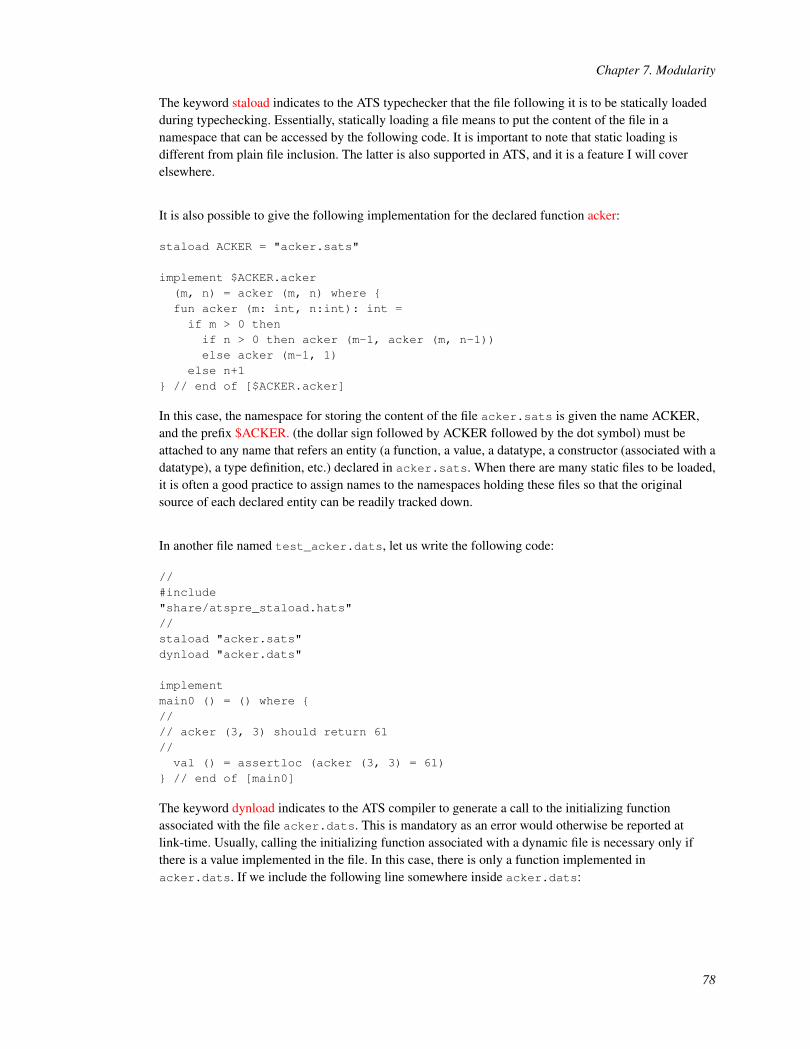
Chapter 7. Modularity
The keyword staload indicates to the ATS typechecker that the file following it is to be statically loadedduring typechecking. Essentially, statically loading a file means to put the content of the file in anamespace that can be accessed by the following code. It is important to note that static loading isdifferent from plain file inclusion. The latter is also supported in ATS, and it is a feature I will coverelsewhere.
It is also possible to give the following implementation for the declared function acker:
staload ACKER = "acker.sats"
implement $ACKER.acker(m, n) = acker (m, n) where {fun acker (m: int, n:int): int =if m > 0 thenif n > 0 then acker (m-1, acker (m, n-1))else acker (m-1, 1)
else n+1} // end of [$ACKER.acker]
In this case, the namespace for storing the content of the file acker.sats is given the name ACKER,and the prefix $ACKER. (the dollar sign followed by ACKER followed by the dot symbol) must beattached to any name that refers an entity (a function, a value, a datatype, a constructor (associated with adatatype), a type definition, etc.) declared in acker.sats. When there are many static files to be loaded,it is often a good practice to assign names to the namespaces holding these files so that the originalsource of each declared entity can be readily tracked down.
In another file named test_acker.dats, let us write the following code:
//#include"share/atspre_staload.hats"//staload "acker.sats"dynload "acker.dats"
implementmain0 () = () where {//// acker (3, 3) should return 61//val () = assertloc (acker (3, 3) = 61)
} // end of [main0]
The keyword dynload indicates to the ATS compiler to generate a call to the initializing functionassociated with the file acker.dats. This is mandatory as an error would otherwise be reported atlink-time. Usually, calling the initializing function associated with a dynamic file is necessary only ifthere is a value implemented in the file. In this case, there is only a function implemented inacker.dats. If we include the following line somewhere inside acker.dats:
78

Chapter 7. Modularity
#define ATS_DYNLOADFLAG 0 // no need for dynloading at run-time
then the line starting with the keyword dynload in test_acker.dats is no longer needed. The functionassertloc verifies at run-time that its argument evaluates to the boolean value true. In the case where theargument evaluates to false, the function call aborts and a message is reported that contains the name ofthe file, which is test_acker.dats in this example, and the location at which the source code of thecall is found in the file. If this sounds a bit confusing, please try to execute a program that contains a callto assertloc on false and you will see clearly what happens.
The simplest way to compile the two files acker.dats and test_acker.dats is to issue the followingcommand-line:
atscc -o test_acker acker.dats test_acker.dats
The generated excutable test_acker is in the current working directory. The compilation can also beperformed separately as is demonstrated below:
atscc -c acker.datsatscc -c test_acker.datsatscc -o test_acker acker_dats.o test_acker_dats.o
This style of separate compilation works particularly well when it is employed by the make utility.
If we want to, we can also merge acker.sats and acker.dats into a single filename of the followingcontent:
externfun acker (m: int, m: int): int
implementacker (m, n) =if m > 0 thenif n > 0 then acker (m-1, acker (m, n-1))else acker (m-1, 1)
else n+1// end of [acker]
Suppose that this single file is given the name acker3.dats. Then the testing code can be written asfollows:
//#include"share/atspre_staload.hats"//staload "acker3.dats"dynload "acker3.dats"
implementmain0 () = () where {
79

Chapter 7. Modularity
//// acker (3, 3) should return 61//val () = assertloc (acker (3, 3) = 61)
} // end of [main0]
Note that it is perfectly fine for a dynamic ATS file to be statically loaded. Actually, a static ATS file isreally just a special case of dynamic ATS file in which there is no implementation (of either functions orvalues).
7.3. Generic Template Implementation
Interfaces for function templates are mostly similar to those for functions. For example, the followingsyntax declares an interface in a dynamic file for a function template of the name list0_fold_left:
externfun{a:t0p}{b:t0p} list0_fold_left(xs: list0 b, f: (a, b) -<cloref1> a, init: a): a
where t0p is a shorthand for t@ype.
If the same interface is declared in a static file, the keyword extern should be dropped. Implementing aninterface for a function template is also mostly similar to implementing one for a function. The aboveinterface for list0_fold_left is given an implementation in the following code:
implement{a}{b}list0_fold_left(xs, f, init) = let
//fun loop(xs: list0 b, res: a
) : a =(case+ xs of| list0_nil () => res| list0_cons (x, xs) => loop (xs, f (res, x))
) (* end of [loop] *)//inloop (xs, init)
end // end of [list0_fold_left]
Note that template parameters are required to appear immediately after the keyword implement, and theycannot be omitted. Template parameters can also be passed sequentially as is shown in the followingshort example:
80

Chapter 7. Modularity
externfun{a,b:t0p}{c:t0p}app2 (f: (a, b) -<cloref1> c, x: a, y: b): c
implement{a,b}{c} app2 (f, x, y) = f (x, y)
The style of template implementation presented in this section is referred to as generic templateimplementation. I will later present a different style of template implementation, which is often referredto as specific template implementation.
7.4. Specific Template Implementation
Implementing an interface for a function template specifically means to give an implementation for afixed instance of the template. For instance, the following interface is for a function template of the nameeq_elt_elt:
fun{a:t0p}eq_elt_elt (x: a, y: a): bool // a generic equality
There is no meaningful generic implementation for eq_elt_elt as equality test for values of a type Tdepends on T. Two specific template implementations are given as follows for the instanceseq_elt_elt<int> and eq_elt_elt<double>:
implement eq_elt_elt<int> (x, y) = g0int_eq (x, y)implement eq_elt_elt<double> (x, y) = g0float_eq (x, y)
where eq_int_int and eq_double_double are equality functions for values of the type int and double,respectively. It is also possible to give the implementations as follows:
implement eq_elt_elt<int> (x, y) = (x = y)implement eq_elt_elt<double> (x, y) = (x = y)
This is allowed as the symbol = is already overloaded with g0int_eq and g0float_eq (in addition to manyother functions).
Let us now see a typical use of specific template implementation. The following defined functiontemplate listeq implements an equality function on lists:
fun{a:t0p} listeq(xs: list0 a
81

Chapter 7. Modularity
, ys: list0 a) : bool = (case+ (xs, ys) of| (list0_cons (x, xs),
list0_cons (y, ys)) =>if eq_elt_elt<a> (x, y) then listeq (xs, ys) else false
| (list0_nil (), list0_nil ()) => true| (_, _) => false
) (* end of [listeq] *)
Given two lists xs and ys, listeq returns true if and only if xs and ys are of the same length and eachelement in xs equals the corresponding one in ys (according to eq_elt_elt). Given a type T, it is clear thatthe instance eq_elt_elt<T> is needed if listeq is called on two lists of the type list0(T). In other words, aspecific implementation for eq_elt_elt<T> should be given if a call to listeq is to be made on two lists ofthe type list0(T). Note that the implementation for an instance of a function template is required to beaccessible from the file where the instance is called.
As a comparison, the following defined function template listeqf also implements equality test on twogiven lists:
fun{a:t0p} listeqf(xs: list0 a
, ys: list0 a, eq: (a, a) -> bool) : bool = (case+ (xs, ys) of| (list0_cons (x, xs),
list0_cons (y, ys)) =>if eq (x, y) then listeqf (xs, ys, eq) else false
| (list0_nil (), list0_nil ()) => true| (_, _) => false
) (* end of [listeqf] *)
In this case, listeqf takes an additional argument eq that tests whether two list elements are equal. Aslisteq is a first-order function while listeqf is a higher-order one, it is likely for the former to be compiledinto more efficient object code. I would like to point out that the library of ATS makes pervasive use ofspecifically implemented templates.
Please find the code presented in this section plus some additional testing code available on-line(https://github.com/ats-lang/ats-lang.github.io/blob/master/DOCUMENT/INT2PROGINATS/CODE/CHAP_MODULARITY/listeq.dats).
82

Chapter 7. Modularity
7.5. Abstract Types
The name abstract type refers to a type such that values of the type are represented in a way that iscompletely hidden from users of the type. This form of information-hiding attempts to ensure thatchanges to the implementation of an abstract type cannot introduce type-errors into well-typed code thatmakes use of the abstract type. In ATS as well as in many other programming languages, abstract typesplay a pivotal role in support of modular programming. I will present as follows a concrete example toillustrate a typical use of abstract types in practice.
Suppose that we are to implement a package to provide various funtionalities on finite sets of integers.We first declare an abstract type intset as follows for values representing finite sets of integers:
abstype intset // a boxed abstract type
The keyword abstype indicates that the declared abstract type intset is boxed, that is, the size of intset isthe same as that of a pointer. There is a related keyword abst@ype for introducing unboxed abstracttypes, which will be explained elsewhere. We next present an interface for each function or value that wewant to implement in the package:
// empty setval intset_empty : intset
// singleton set of [x]fun intset_make_sing (x: int): intset
// turning a list into a setfun intset_make_list (xs: list0 int): intset
// turning a set into a listfun intset_listize (xs: intset): list0 (int)
// membership testfun intset_ismem (xs: intset, x: int): bool
// computing the size of [xs]fun intset_size (xs: intset): size_t
// adding [x] into [xs]fun intset_add (xs: intset, x: int): intset
// deleting [x] from [xs]fun intset_del (xs: intset, x: int): intset
// union of [xs1] and [xs2]fun intset_union (xs1: intset, xs2: intset): intset
// intersection of [xs1] and [xs2]fun intset_inter (xs1: intset, xs2: intset): intset
// difference between [xs1] and [xs2]
83

Chapter 7. Modularity
fun intset_differ (xs1: intset, xs2: intset): intset
Let us now suppose that the declaration for intset and the above interfaces are all stored in a file namedintset.sats (or any other legal name for a static file).
Usually, a realistic implementation for finite sets is based on some kind of balanced trees (e.g., AVLtrees, red-black trees). For the purpose of illustration, I hereby give an implementation in which finitesets of integers are represented as ordered lists of integers. This implementation is contained in a filenamed intset.dats, which is available on-line (https://github.com/ats-lang/ats-lang.github.io/blob/master/DOCUMENT/INT2PROGINATS/CODE/CHAP_MODULARITY/intset.dats).In order to construct values of an abstract type, we need to concretize it temporarily by using thefollowing form of declaration:
assume intset = list0 (int)
where assume is a keyword. This assume-declaration equates intset with the type list0 (int) and thisequation is valid until the end of the scope in which it is introduced. As the assume-declaration is at thetoplevel in intset.dats, the assumption that intset equals list0 (int) is valid until the end of the file.There is a global restriction in ATS that allows each abstract type to be concretized by anassume-declaration at most once. More specifically, if an abstract type is concretized in two filesfoo1.dats and foo2.dats, then these two files cannot be used together to generate an executable. Therest of implementation in intset is all standard. For instance, the union operation on two given sets ofintegers is implemented as follows:
implementintset_union(xs1, xs2) = (
case+ (xs1, xs2) of| (list0_cons (x1, xs11),
list0_cons (x2, xs21)) =>letval sgn = compare (x1, x2)
incase+ 0 of| _ when sgn < 0 =>
list0_cons{int}(x1, intset_union (xs11, xs2))| _ when sgn > 0 =>
list0_cons{int}(x2, intset_union (xs1, xs21))| _ (* sgn = 0 *) =>
list0_cons{int}(x1, intset_union (xs11, xs21))// end of [case]
end // end of [(cons, cons)]| (list0_nil (), _) => xs2| (_, list0_nil ()) => xs1) (* end of [intset_union] *)
There is also some testing code available on-line (https://github.com/ats-lang/ats-lang.github.io/blob/master/DOCUMENT/INT2PROGINATS/CODE/CHAP_MODULARITY/test_intset.dats)that makes use of some functions declared in intset.sats. Often testing code as such is constructedimmediately after the interfaces for various functions and values in a package are declared. This allows
84

Chapter 7. Modularity
these interfaces to be tried before they are actually implemented so that potential flaws can be exposed ina timely fashion.
7.6. Example: A Package for Rationals
Let us represent a rational number as a pair of integers. If we declare a boxed abstract type rat for valuesrepresenting rational numbers, then each value of the type rat is stored in heap-allocated memory, whichcan only be reclaimed through garbage collection (GC). Instead, we follow an alternative approach bydeclaring rat as an unboxed abstract type. Therefore, a declaration like the following one is expected:
abst@ype rat
The problem with this declaration is that it is too abstract. As there is not information given about thesize of the type rat, the ATS compiler does not even know how much memory is needed for storing avalue of the type rat. However, the programmer should not assume that such a form of declaration isuseless. There are realistic circumstances where a declaration of this form can be of great importance,and this is a topic I will cover elsewhere. For now, let us declare an unboxed abstract type as follows:
abst@ype rat = (int, int)
This declaration simply informs the ATS compiler that the representation for values of the type rat is thesame as the one for values of the type (int, int). However, this information is not made available to thetypechecker of ATS. In particular, if a value of the type rat is treated as a pair of integers in a program,then a type-error will surely occur.
The following code is contained in a file named ratmod.sats, which is available on-line(https://github.com/ats-lang/ats-lang.github.io/blob/master/DOCUMENT/INT2PROGINATS/CODE/CHAP_MODULARITY/ratmod.sats).
exception Denominatorexception DivisionByZero
fun rat_make_int_int (p: int, q: int): rat
fun ratneg: (rat) -> rat // negationfun ratadd: (rat, rat) -> rat // additionfun ratsub: (rat, rat) -> rat // subtractionfun ratmul: (rat, rat) -> rat // multiplicationfun ratdiv: (rat, rat) -> rat // division
The exception Denominator is for reporting an erroneous occasion where a rational number is to beformed with a denominator equal to zero. Given two integers representing the numerator anddenominator of a rational number, the function rat_make_int_int returns a value representing the rationalnumber. The following implementation of rat_make_int_int can be found in a file named ratmod.dats,
85

Chapter 7. Modularity
which is also available on-line (https://github.com/ats-lang/ats-lang.github.io/blob/master/DOCUMENT/INT2PROGINATS/CODE/CHAP_MODULARITY/ratmod.dats).
implementrat_make_int_int (p, q) = letfun make (p: int, q: int
) : rat = letval r = gcd (p, q) in (p / r, q / r)
end // end of [make]//val () = if q = 0 then $raise Denominator
//inif q > 0 then make (p, q) else make (~p, ~q)
end // end of [rat_make_int_int]
Given a pair of integers p and q such that q is not zero, the function rat_make_int_int returns another pairof integers p
1and q
1such that q
1is positive, p
1and q
1are coprimes, that is, their greatest common divisor
is 1, and p1/q
1equals p/q. With rat_make_int_int, it is straightforward to implement as follows the
arithmetic operations on rational numbers:
implement ratneg (x) = (~x.0, x.1)
implementratadd (x, y) =rat_make_int_int (x.0 * y.1 + x.1 * y.0, x.1 * y.1)
// end of [ratadd]
implementratsub (x, y) =rat_make_int_int (x.0 * y.1 - x.1 * y.0, x.1 * y.1)
// end of [ratsub]
implementratmul (x, y) = rat_make_int_int (x.0 * y.0, x.1 * y.1)
implementratdiv (x, y) = (if y.0 > 0then rat_make_int_int (x.0 * y.1, x.1 * y.0) else $raise DivisionByZero()
// end of [if]) (* end of [ratdiv] *)
There is also some testing code available on-line (https://github.com/ats-lang/ats-lang.github.io/blob/master/DOCUMENT/INT2PROGINATS/CODE/CHAP_MODULARITY/test_ratmod.dats)that makes use of some functions declared in ratmod.sats.
86

Chapter 7. Modularity
7.7. Example: A Functorial Package for Rationals
The previous package for rational numbers contains a serious limitation: The type for the integersemployed in the representation of rational numbers is fixed to be int. If we ever want to represent rationalnumbers based on integers of a different type (for instance, lint for long integers or llint for long longintegers), then we need to implement another package for rationals based on such integers. It is clearlyadvantageous to avoid this style of programming as it involves code duplication to a great extent.
The approach I employ in this section to implement a package for rational numbers that can address theaforementioned limitation follows the idea of functors in the programming language Standard ML(SML). Let us first introduce a type definition as follows:
typedefintmod (a:t@ype) = ’{ofint= int -> a
, fprint= (FILEref, a) -> void, neg= (a) -> a // negation, add= (a, a) -> a // addition, sub= (a, a) -> a // subtraction, mul= (a, a) -> a // multiplication, div= (a, a) -> a // division, mod= (a, a) -> a // modulo operation, cmp= (a, a) -> int // comparison} // end of [intmod]
Given a type T, intmod(T) is a boxed record type in which each field is a function type. A value of thetype intmod(T) is supposed to represent a module of integer operations on integers represented by valuesof the type T. Similarly, let us introduce another type definition as follows:
abst@ype rat(a:t@ype) = (a, a)
typedefratmod (a:t@ype) = ’{make= (a, a) -<cloref1> rat a
, fprint= (FILEref, rat a) -<cloref1> void, numer= rat a -> a // numerator, denom= rat a -> a // denominator, neg= (rat a) -<cloref1> rat a // negation, add= (rat a, rat a) -<cloref1> rat a // addition, sub= (rat a, rat a) -<cloref1> rat a // subtraction, mul= (rat a, rat a) -<cloref1> rat a // multiplication, div= (rat a, rat a) -<cloref1> rat a // division, cmp= (rat a, rat a) -<cloref1> int // comparison} // end of [ratmod]
Given a type T, a value of the type ratmod(T) is supposed to represent a module of rational operations onrationals represented by values of the type rat(T). The function we need to implement can now be giventhe following interface:
87

Chapter 7. Modularity
fun{a:t@ype}ratmod_make_intmod (int: intmod a): ratmod a
If applied to a given module of integer operations, ratmod_make_intmod returns a module of rationaloperations such that the integers in the former and the latter modules have the same representation.Therefore, ratmod_make_intmod behaves like a functor in SML. In the following code, let us implementtwo modules ratmod_int and ratmod_dbl of rational operations in which integers are represented asvalues of the types int and double, respectively:
staload M = "libc/SATS/math.sats"
val ratmod_int = let//val intmod_int = ’{ofint= lam (i) => i
, fprint= lam (out, x) => $extfcall (void, "fprintf", out, "%i", x), neg= lam (x) => ~x, add= lam (x, y) => x + y, sub= lam (x, y) => x - y, mul= lam (x, y) => x * y, div= lam (x, y) => x / y, mod= lam (x, y) => op mod (x, y), cmp= lam (x, y) => compare (x, y)} : intmod (int) // end of [val]//inratmod_make_intmod<int> (intmod_int)
end // end of [val]
val ratmod_dbl = let//val intmod_dbl = ’{ofint= lam (i) => g0i2f(i)
, fprint= lam (out, x) => $extfcall (void, "fprintf", out, "%0.f", x), neg= lam (x) => ~x, add= lam (x, y) => x + y, sub= lam (x, y) => x - y, mul= lam (x, y) => x * y, div= lam (x, y) => $M.trunc (x / y) // truncation, mod= lam (x, y) => $M.fmod (x, y), cmp= lam (x, y) => compare (x, y)} : intmod (double) // end of [val]//inratmod_make_intmod<double> (intmod_dbl)
end // end of [ratmod_dbl]
Animplementation of the function ratmod_make_intmod is available on-line (https://github.com/ats-lang/ats-lang.github.io/blob/master/DOCUMENT/INT2PROGINATS/CODE/CHAP_MODULARITY/ratfun.dats)
88

Chapter 7. Modularity
and there is some related testing code available on-line (https://github.com/ats-lang/ats-lang.github.io/blob/master/DOCUMENT/INT2PROGINATS/CODE/CHAP_MODULARITY/test_ratfun.dats)as well.
89
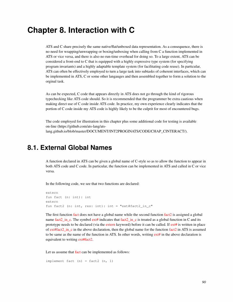
Chapter 8. Interaction with C
ATS and C share precisely the same native/flat/unboxed data representation. As a consequence, there isno need for wrapping/unwrapping or boxing/unboxing when calling from C a function implemented inATS or vice versa, and there is also no run-time overhead for doing so. To a large extent, ATS can beconsidered a front-end to C that is equipped with a highly expressive type system (for specifyingprogram invariants) and a highly adaptable template system (for facilitating code reuse). In particular,ATS can often be effectively employed to turn a large task into subtasks of coherent interfaces, which canbe implemented in ATS, C or some other langauges and then assembled together to form a solution to theorginal task.
As can be expected, C code that appears directly in ATS does not go through the kind of rigoroustypechecking like ATS code should. So it is recommended that the programmer be extra cautious whenmaking direct use of C code inside ATS code. In practice, my own experience clearly indicates that theportion of C code inside my ATS code is highly likely to be the culprit for most of encountered bugs.
The code employed for illustration in this chapter plus some additional code for testing is availableon-line (https://github.com/ats-lang/ats-lang.github.io/blob/master/DOCUMENT/INT2PROGINATS/CODE/CHAP_CINTERACT/).
8.1. External Global Names
A function declared in ATS can be given a global name of C-style so as to allow the function to appear inboth ATS code and C code. In particular, the function can be implemented in ATS and called in C or viceversa.
In the following code, we see that two functions are declared:
externfun fact (n: int): intexternfun fact2 (n: int, res: int): int = "ext#fact2_in_c"
The first function fact does not have a global name while the second function fact2 is assigned a globalname fact2_in_c. The symbol ext# indicates that fact2_in_c is treated as a global function in C and itsprototype needs to be declared (via the extern keyword) before it can be called. If ext# is written in placeof ext#fact2_in_c in the above declaration, then the global name for the function fact2 in ATS is assumedto be same as the name of the function in ATS. In other words, writing ext# in the above declaration isequivalent to writing ext#fact2.
Let us assume that fact can be implemented as follows:
implement fact (n) = fact2 (n, 1)
90

Chapter 8. Interaction with C
When compiling this implementation, the ATS compiler needs to form function names in the generatedC code to refer to fact and fact2. For the former, the function name in the C code is determined by a setof rules (which take into account the issue of namespace). For the latter, the function name is simplychosen to be the assigned global name fact2_in_c. As is suggested by the name of fact2_in_c, thisfunction can be directly implemented in C as follows:
intfact2_in_c (int n, int res){while (n > 0) { res *= n ; n -= 1 ; } ; return res ;
}
It is also allowed to implement fact2 in ATS directly as is shown below:
implementfact2 (n, res) = if n > 0 then fact2 (n-1, n*res) else res
This implementation of fact2 can be called in C through the name fact2_in_c.
If both fact2 and fact2_in_c are implemented (the former in ATS and the latter in C), then a link-timeerror is to be issued to indicate that fact2_in_c is implemented repeatedly.
One can also declare fact2 as follows:
externfun fact2 (n: int, res: int): int = "mac#fact2_in_c"
The symbol mac# indicates that fact2_in_c is treated like a macro in C. In particular, fact2_in_c can becalled without its prototype being declared first. As a matter of fact, it may not even have a prototype.This style of declaration naturally expects fact2_in_c to be implemented in C directly.
It is also allowed to use sta# in place of mac#:
externfun fact2 (n: int, res: int): int = "sta#fact2_in_c"
If declared in this style, which only occurs rarely in practice, then fact2_in_c is treated like a staticfunction in C.
For the sake of completeness, I mention as follows another way of declaring a static function:
static fun fact2 (n: int, res: int): int
This style of declaration is automatically translated into the following one:
extern fun fact2 (n: int, res: int): int = "sta#"
91

Chapter 8. Interaction with C
where the use of sta# means that the name referring to fact2 in C is simply fact2.
8.2. External Types and Values in ATS
External types and values can be readily formed in ATS to refer to types and values declared in C.
Suppose that there is a type in C of the name some_type_in_c, then this type can be referred to in ATS as$extype"some_type_in_c". For instance, type definitions are introduced in the following code for someexternal types in C:
typedef Cint = $extype"int"typedef Clint = $extype"long int"typedef Cllint = $extype"long long int"typedef Cint2 = $extype"struct{ int x; int y; }"
Suppose that there is a value in C of the name some_value_in_c, then this value can be referred to in ATSas $extval(T, "some_value_in_c"), where T is a type in ATS assigned to this value. For instance, macrodefinitions are introduced in the following code for some external values in C:
macdef NULL = $extval(ptr, "0")macdef stdin_ref = $extval(FILEref, "stdin")macdef stdout_ref = $extval(FILEref, "stdout")
External values can also be formed to refer to functions in C as done in the following code:
macdef atoi = $extval(string -> int, "atoi")macdef atol = $extval(string -> lint, "atol")macdef atof = $extval(string -> double, "atof")
Note that there are other ways in ATS that are often more approriate for directly referring to functions inC. Typically, the primary purpose of forming an external value in ATS is to allow a constant declared inC to be directly referred to in ATS code.
8.3. Inclusion of External Code in ATS
Just like including assembly code inside C code, it is straightforward to include C code inside ATS code.For instance, the example appearing at the beginning of this chapter can be written as follows in a singlefile:
//externfun fact (n: int): intexternfun fact2 (n: int, res: int): int = "ext#fact2_in_c"
92
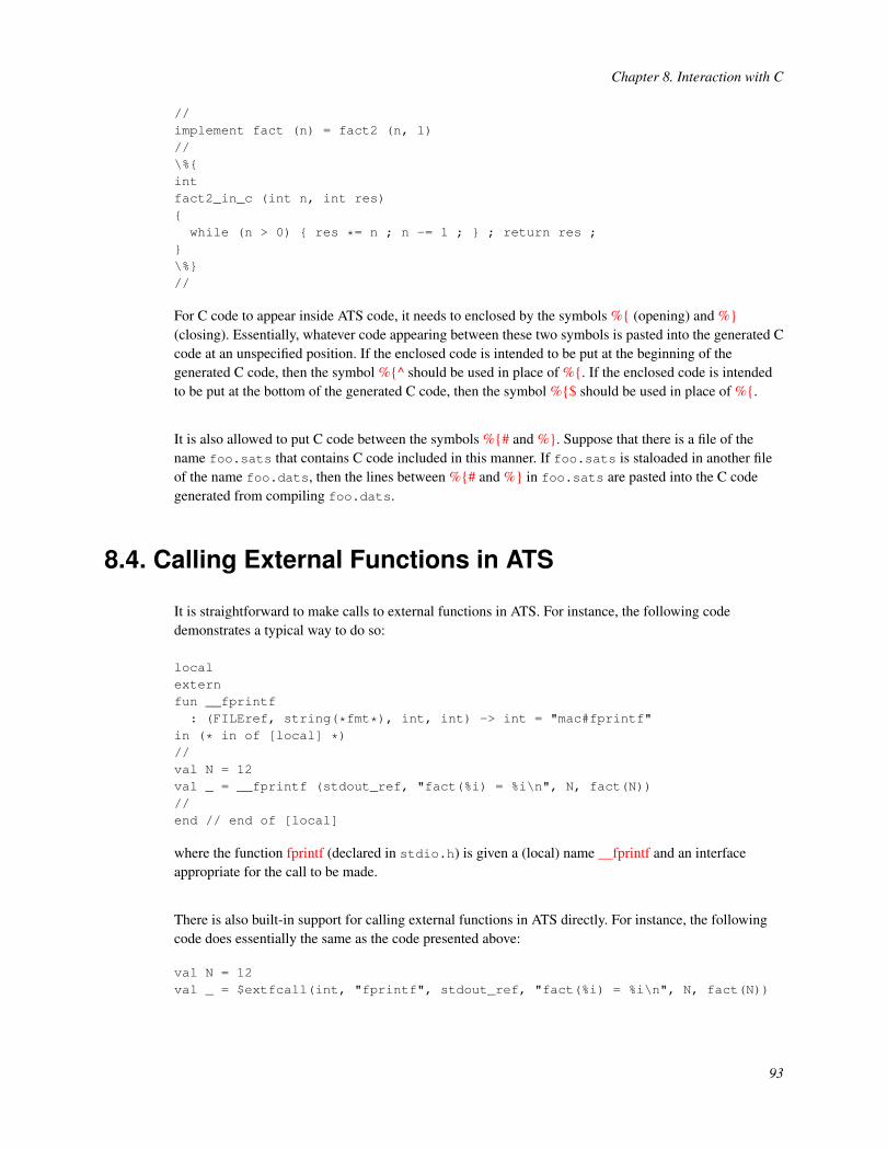
Chapter 8. Interaction with C
//implement fact (n) = fact2 (n, 1)//\%{intfact2_in_c (int n, int res){while (n > 0) { res *= n ; n -= 1 ; } ; return res ;
}\%}//
For C code to appear inside ATS code, it needs to enclosed by the symbols %{ (opening) and %}(closing). Essentially, whatever code appearing between these two symbols is pasted into the generated Ccode at an unspecified position. If the enclosed code is intended to be put at the beginning of thegenerated C code, then the symbol %{^ should be used in place of %{. If the enclosed code is intendedto be put at the bottom of the generated C code, then the symbol %{$ should be used in place of %{.
It is also allowed to put C code between the symbols %{# and %}. Suppose that there is a file of thename foo.sats that contains C code included in this manner. If foo.sats is staloaded in another fileof the name foo.dats, then the lines between %{# and %} in foo.sats are pasted into the C codegenerated from compiling foo.dats.
8.4. Calling External Functions in ATS
It is straightforward to make calls to external functions in ATS. For instance, the following codedemonstrates a typical way to do so:
localexternfun __fprintf: (FILEref, string(*fmt*), int, int) -> int = "mac#fprintf"
in (* in of [local] *)//val N = 12val _ = __fprintf (stdout_ref, "fact(%i) = %i\n", N, fact(N))//end // end of [local]
where the function fprintf (declared in stdio.h) is given a (local) name __fprintf and an interfaceappropriate for the call to be made.
There is also built-in support for calling external functions in ATS directly. For instance, the followingcode does essentially the same as the code presented above:
val N = 12val _ = $extfcall(int, "fprintf", stdout_ref, "fact(%i) = %i\n", N, fact(N))
93

Chapter 8. Interaction with C
When $extfcall is employed to make an external function call, its first argument is the return type of thecall, and its second argument is the name of the called function (represented as a string), and its rest ofarguments are the arguments of the called function.
8.5. Unsafe C-style Programming in ATS
ATS is probably not a programming language easy for one to write code in. While ATS provides manyfeatures to support safe (low-level) programming, it may take a long time and some great efforts for aprogrammer to learn and then master these features before he or she can make effective use of them. Inthis section, I would like to present some ATS code written in C-style that makes typical use of certanunsafe programming features in ATS. This is a programming style that should be familiar to anyprogrammer who can write C code competently.
There are always occasions where one may find it sensible to program in unsafe C-style. Sometimes, onejust wants to get a running implementation and then relies on testing to detect and fix bugs. Sometimes,one simply does not know enough of ATS needed to implement a function in a safe programmingmanner. This list of occasions can be readily extended as one wishes. I myself do unsafe C-styleprogramming in ATS frequently, and I see it as a necessary skill for anyone who not just only wants to beable to write code in ATS but also wants to do it highly productively. Let us now see a concrete exampleof unsafe C-style programming in ATS.
Suppose that we want to implement a function for comparing two given strings according to the standardlexicographic ordering. Let us name the function strcmp and give it the following interface:
fun strcmp (str1: string, str2: string): int
Given two strings str1 and str2, strcmp(str1, str2) is expected to return 1, -1, and 0 if str1 is greater than,less than, and equal to str2, respectively. An implementation of strcmp is given as follows:
staloadUN = "prelude/SATS/unsafe.sats"
(* ****** ****** *)
implementstrcmp (str1, str2) = let//funloop(p1: ptr, p2: ptr
) : int = let//val c1 = $UN.ptr0_get<uchar>(p1)val c2 = $UN.ptr0_get<uchar>(p2)//
94

Chapter 8. Interaction with C
incase+ 0 of| _ when c1 > c2 => 1| _ when c1 < c2 => ~1| _ (* c1 = c2 *) =>(if $UN.cast{int}(c1) = 0then 0 else loop (ptr0_succ<uchar>(p1), ptr0_succ<uchar>(p2))
// end of [if])
end (* end of [loop] *)//inloop (string2ptr(str1), string2ptr(str2))
end (* end of [strcmp] *)
For a programmer familar with C, the above implementation of strcmp should be easily accessible. Thereare a variety of unsafe functions declared in unsafe.sats (https://github.com/ats-lang/ats-lang.github.io/blob/master/DOCUMENT/ATS-Postiats/prelude/SATS/unsafe.sats). Given a type T and apointer p, ptr0_get<T>(p) fetches the value of the type T stored at the location to which p points. Notethat ptr0_get is inherently unsafe as there is simply no guarantee that p actually points to a valid memorylocation where a value of the type T is stored. The function cast, which is also inherently unsafe, caststhe type of a given value into any chosen type. The function template ptr0_succ, which is declared inpointer.sats (https://github.com/ats-lang/ats-lang.github.io/blob/master/DOCUMENT/ATS-Postiats/prelude/SATS/pointer.sats), is type-safe. Given a type T, ptr0_succ<T>(p) returns the pointerthat is n bytes after p, where n equals the size of T.
Please find the entire code for this example on-line (https://github.com/ats-lang/ats-lang.github.io/blob/master/DOCUMENT/INT2PROGINATS/CODE/CHAP_CINTERACT/strcmp.dats).
For a function like strcmp, one can readily implement it in C directly. For instance, an implementation ofstrcmp in C, which is essentially a translation of the above implementation of strcmp in ATS, is given asfollows:
int strcmp (char *p1, char *p2){int res ;unsigned char c1, c2;while (1){c1 = *p1; c2 = *p2;if (c1 > c2) { res = 1; break; } ;if (c1 < c2) { res = -1; break; } ;if ((int)c1==0) { res = 0 ; break ; } else { p1++; p2++; } ;
}return res ;
}
However, writing ATS code in C-style can often have advantages over writing C code directly. Forinstance, there is direct support in ATS but not in C for implementing function templates. In C, one is
95
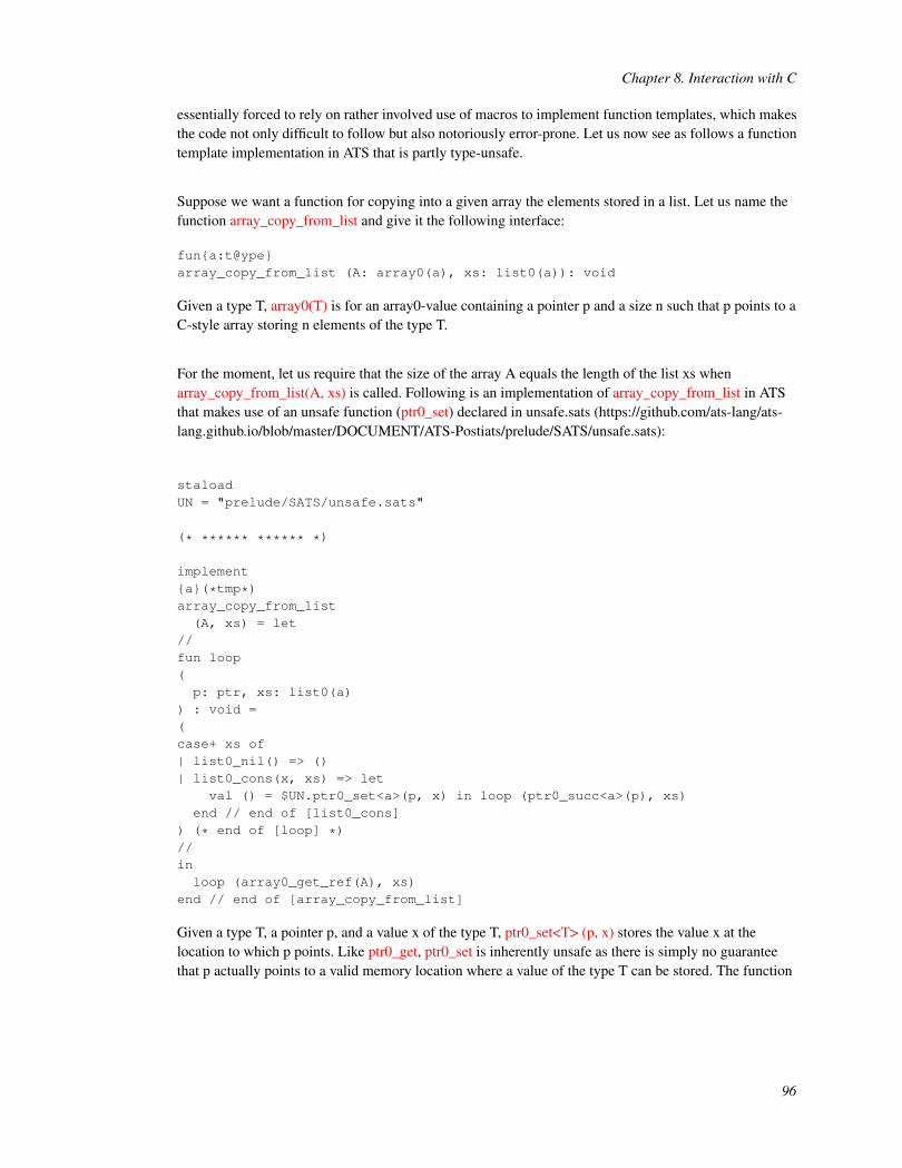
Chapter 8. Interaction with C
essentially forced to rely on rather involved use of macros to implement function templates, which makesthe code not only difficult to follow but also notoriously error-prone. Let us now see as follows a functiontemplate implementation in ATS that is partly type-unsafe.
Suppose we want a function for copying into a given array the elements stored in a list. Let us name thefunction array_copy_from_list and give it the following interface:
fun{a:t@ype}array_copy_from_list (A: array0(a), xs: list0(a)): void
Given a type T, array0(T) is for an array0-value containing a pointer p and a size n such that p points to aC-style array storing n elements of the type T.
For the moment, let us require that the size of the array A equals the length of the list xs whenarray_copy_from_list(A, xs) is called. Following is an implementation of array_copy_from_list in ATSthat makes use of an unsafe function (ptr0_set) declared in unsafe.sats (https://github.com/ats-lang/ats-lang.github.io/blob/master/DOCUMENT/ATS-Postiats/prelude/SATS/unsafe.sats):
staloadUN = "prelude/SATS/unsafe.sats"
(* ****** ****** *)
implement{a}(*tmp*)array_copy_from_list(A, xs) = let
//fun loop(p: ptr, xs: list0(a)
) : void =(case+ xs of| list0_nil() => ()| list0_cons(x, xs) => let
val () = $UN.ptr0_set<a>(p, x) in loop (ptr0_succ<a>(p), xs)end // end of [list0_cons]
) (* end of [loop] *)//inloop (array0_get_ref(A), xs)
end // end of [array_copy_from_list]
Given a type T, a pointer p, and a value x of the type T, ptr0_set<T> (p, x) stores the value x at thelocation to which p points. Like ptr0_get, ptr0_set is inherently unsafe as there is simply no guaranteethat p actually points to a valid memory location where a value of the type T can be stored. The function
96

Chapter 8. Interaction with C
array0_get_ref, which is declared in array0.sats (https://github.com/ats-lang/ats-lang.github.io/blob/master/DOCUMENT/ATS-Postiats/libats/ML/SATS/array0.sats), returns the pointerto the C-style array associated with a given array0-value.
Please find the entire code for this example on-line (https://github.com/ats-lang/ats-lang.github.io/blob/master/DOCUMENT/INT2PROGINATS/CODE/CHAP_CINTERACT/ArrayCopyFromList.dats).
8.6. Exporting Types in ATS for Use in C
There is also support in ATS for exporting types to make them available for use in C directly. In thefollowing example, a typedef of the name int_and_string is expected to be declared in the generated Ccode for values that are assigned the type (int, string) in ATS:
externtypedef "int_and_string" = (int, string)
Essentially, int_and_string is defined in C as follows:
typedefstruct {int atslab__0; void *atslab__1;
} int_and_string ;
Sometimes, we want to construct in C values of a datatype declared in ATS. For instance, let us try toconstruct a value of the form cons2(i, d) in C for an integer i and a double d, where cons2 is a dataconstructor associated with the following declared datatype abc:
datatype abc =| cons1 of int | cons2 of (int, double)
Whenever a data constructor is declared, a corresponding (linear) type constructor is created whose nameequals the concatenation of the name of the data constructor and the string "_pstruct". So in the case ofthe above declared datatype abc, the type constructors cons1_pstruct and cons2_pstruct are created, andthese type constructors can be used to form types for boxed values constructed with the data constructorscons1 and cons2.
In the following declaration, the type cons2_pstruct(int, double) in ATS is exported to C under the namecons2_node:
externvtypedef "cons2_node" = cons2_pstruct(int, double)
Implicitly, a typedef in C of the name cons2_node_ is also introduced for the unboxed portion of a valueconstructed with the data constructor cons2. Essentially, we have the following generated code in C:
97
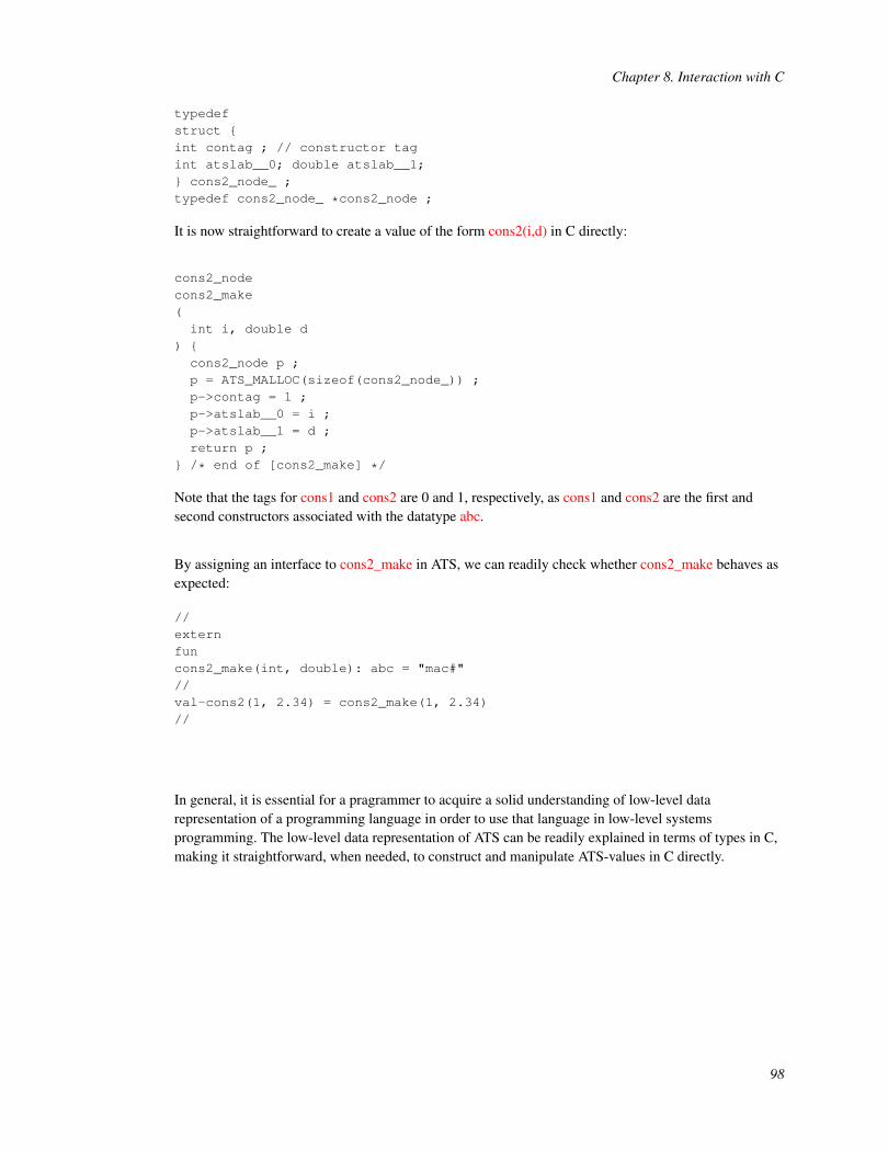
Chapter 8. Interaction with C
typedefstruct {int contag ; // constructor tagint atslab__0; double atslab__1;} cons2_node_ ;typedef cons2_node_ *cons2_node ;
It is now straightforward to create a value of the form cons2(i,d) in C directly:
cons2_nodecons2_make(int i, double d
) {cons2_node p ;p = ATS_MALLOC(sizeof(cons2_node_)) ;p->contag = 1 ;p->atslab__0 = i ;p->atslab__1 = d ;return p ;
} /* end of [cons2_make] */
Note that the tags for cons1 and cons2 are 0 and 1, respectively, as cons1 and cons2 are the first andsecond constructors associated with the datatype abc.
By assigning an interface to cons2_make in ATS, we can readily check whether cons2_make behaves asexpected:
//externfuncons2_make(int, double): abc = "mac#"//val-cons2(1, 2.34) = cons2_make(1, 2.34)//
In general, it is essential for a pragrammer to acquire a solid understanding of low-level datarepresentation of a programming language in order to use that language in low-level systemsprogramming. The low-level data representation of ATS can be readily explained in terms of types in C,making it straightforward, when needed, to construct and manipulate ATS-values in C directly.
98

Chapter 8. Interaction with C
8.7. Example: Constructing a Statically Allocated List
In embedded programming, static memory allocation is often preferred due to dynamic memoryallocation being less predictable. I present as follows an example in which a list is constructed withstatically allocated memory. This example also strongly attests to ATS and C being intimately related.
In order to statically allocate memory for list-nodes, we need to first form a type for list-nodes so that wecan inform the C compiler how much memory is needed for each list-node. In the following code, thetype list_node in ATS is for boxed list-nodes, and this type is exported to C under the same name:
//vtypedeflist_node =list_cons_pstruct(int,ptr) // [list_node] for boxed nodes//externvtypedef "list_node" = list_node // exporting [list_node] to C//
Exporting list_node to C also introduces (implicitly) a typedef list_node_ in C for unboxed list-nodes. Sothe following type list_node_ in ATS is precisely what we want (for unboxed list-nodes):
//typedeflist_node_ = $extype"list_node_" // [list_node_] for unboxed nodes//
The following code statically allocates an array of list-nodes and then initialize these nodes, turning thearray into a list:
local
#define N 10
(*** static allocation
*)var nodes = @[list_node_][N]()
fun loop(p: ptr, i: int
) : void = letin//if i < N then letval res =
99

Chapter 8. Interaction with C
$UN.castvwtp0{list_node}(p)val+list_cons (x, xs) = resval () = x := i*ival p = ptr_succ<list_node_> (p)val i = i + 1val () = (if i < N then xs := p else xs := the_null_ptr
) : void // end of [val]val _(*ptr*) = $UN.castvwtp0{ptr}((view@x, view@xs | res))
inloop (p, i)
end else ((*void*)) // end of [if]//end // end of [loop]
in (* in of [local] *)
val () = loop (addr@nodes, 0)val xs_static = $UN.castvwtp0{list(int,N)}((view@nodes|addr@nodes))val () = println! ("xs_static = ", xs_static) // 0, 1, 4, 9, 16, ...
end // end of [local]
The implementation of loop makes extensive use of unsafe C-style programming in ATS. For someonefamiliar with C, it should be straightforward to visualize the C code that corresponds to thisimplementation directly.
Please find the entire code for this example on-line (https://github.com/ats-lang/ats-lang.github.io/blob/master/DOCUMENT/INT2PROGINATS/CODE/CHAP_CINTERACT/StaticAllocList.dats).
100

III. Programming with DependentTypes

Chapter 9. Introduction to Dependent Types
The types we have encountered so far in this book are often not adequately precise in capturingprogramming invariants. For instance, if we assign the type int to both of integers 0 and 1, then wesimply cannot distinguish 0 from 1 at the level of types. This means that 0 and 1 are interchangeable asfar as typechecking is concerned. In other words, we cannot expect a program error to be caught duringtypechecking if the error is caused by 0 being mistyped as 1. This form of imprecision in types canbecome a crippling limitation if we ever want to build a type-based specification language that isreasonably expressive for practical use.
Please find on-line (https://github.com/ats-lang/ats-lang.github.io/blob/master/DOCUMENT/INT2PROGINATS/CODE/CHAP_DEPTYPES/) the codeemployed for illustration in this chapter plus some additional code for testing.
9.1. Enhanced Expressiveness for Specification
The primary purpose of introducing dependent types into the type system of ATS is to greatly enhancethe expressiveness of types so that they can be employed to capture program invariants with muchgreater precision. Generally speaking, dependent types are types dependent on values of expressions. Forinstance, bool is a type constructor in ATS that forms a type bool(b) when applied to a given booleanvalue b. As this type can only be assigned to a boolean expression of the value b, it is often referred to asa singleton type, that is, a type for exactly one value. Clearly, the meaning of bool(b) depends on theboolean value b. Similarly, int is a type constructor in ATS that forms a type int(i) when applied to agiven integer i. This type is also a singleton type as it can only be assigned to an integer expression of thevalue i. Please note that both bool and int are overloaded as they also refer to (non-dependent) types. Iwill gradually introduce many other examples of dependent types. In particular, I will present a flexiblemeans for the programmer to declare dependent datatypes.
The statics of ATS is a simply-typed language, and the types in this language are called sorts so as toavoid some potential confusion (with the types for dynamic terms). The following four listed sorts arecommonly used:
• bool: for static terms of boolean values
• int: for static terms of integer values
• type: for static terms representing boxed types (for dynamic terms)
• t@ype: for static terms representing unboxed types (for dynamic terms)
The sorts bool and int are classified as predicative sorts while the sorts type and t@ype are impredicative.A boxed type is a static term of the sort type while an unboxed type is a static term of the sort t@ype. Astypes, bool and int are static terms of the sort t@ype. As type constructors, bool and int are static termsof the sorts (bool -> t@ype) and (int -> t@ype), respectively. Also note that the type constructor list0 isof the sort (t@ype -> type), which indicates that list0 forms a boxed type when applied to an unboxed
102

Chapter 9. Introduction to Dependent Types
one. There are a variety of built-in static functions in ATS for constructing static terms of the sorts booland int, and I list as follows some of these functions together with the sorts assigned to them:
• ~ (negation): (int) -> int
• + (addition): (int, int) -> int
• - (subtraction): (int, int) -> int
• * (multiplication): (int, int) -> int
• / (division): (int, int) -> int
• > (greater-than): (int, int) -> bool
• >= (greater-than-or-equal-to): (int, int) -> bool
• < (less-than): (int, int) -> bool
• <= (less-than-or-equal-to): (int, int) -> bool
• == (equal-to): (int, int) -> bool
• != (not-equal-to): (int, int) -> bool
• <> (not-equal-to): (int, int) -> bool
• ~ (boolean negation): (bool) -> bool
• || (disjunction): (bool, bool) -> bool
• && (conjunction) : (bool, bool) -> bool
By combining a sort with one or more predicates, we can define a subset sort. For instance, the followingsubset sorts are defined in the file basics_pre.sats (https://github.com/ats-lang/ats-lang.github.io/blob/master/DOCUMENT/ATS-Postiats/prelude/basics_pre.sats), which is automaticallyloaded by the ATS compiler:
sortdef nat = {a: int | a >= 0} // for natural numberssortdef pos = {a: int | a >= 1} // for positive numberssortdef neg = {a: int | a <= ~1} // for negative numbers
sortdef nat1 = {a: nat | a < 1} // for 0sortdef nat2 = {a: nat | a < 2} // for 0, 1sortdef nat3 = {a: nat | a < 3} // for 0, 1, 2sortdef nat4 = {a: nat | a < 4} // for 0, 1, 2, 3
Note that predicates can be sequenced together with the semicolon symbol (;) to form a conjunction:
sortdef nat2 = {a: int | 0 <= a; a < 2} // for 0, 1sortdef nat3 = {a: int | 0 <= a; a < 3} // for 0, 1, 2sortdef sgn = { i:int | ~1 <= i; i <= 1 } // for ~1, 0, 1
It is also possible to define the subset sorts nat2 and nat3 as follows:
sortdef nat2 = {a: int | a == 0 || a == 1} // for 0, 1sortdef nat3 = {a: int | 0 <= a && a <= 2} // for 0, 1, 2
103

Chapter 9. Introduction to Dependent Types
where || and && stands for disjunction and conjunction, respectively.
In order to unleash the expressiveness of dependent types, we need to employ both universal andexistential quantification over static variables. For instance, the type Int in ATS is defined as follows:
typedef Int = [a:int] int (a) // for unspecified integers
where the syntax [a:int] means existential quantification over a static variable a of the sort int.Essentially, this means that for each value of the type Int, there exists an integer I such that the value is ofthe type int(I). Therefore, any value that can be given the type int can also be given the type Int. A typelike Int is often referred to as an existentially quantified type. As another example, the type Nat in ATS isdefined as follows:
typedef Nat = [a:int | a >= 0] int (a) // for natural numbers
where the syntax [a:int | a >= 0] means existential quantification over a static variable a of the sort intthat satisfies the constraint a >= 0. Therefore, each value of the type Nat can be assigned the type int(I)for some integer I satisfying I >= 0. Given that int(I) is a singleton type, the value equals I and is thus anatural number. This means that the type Nat is for natural numbers. The definition of Nat can also begiven as follows:
typedef Nat = [a:nat] int (a) // for natural numbers
where the syntax [a:nat] is just a form of syntactic sugar that automatically expands into [a:int | a >= 0].
At this point, types have already become much more expressive. For instance, we could only assign thetype (int) -> int to a function that maps integers to natural numbers (e.g., the function that computes theabsolute value of a given integer), but we can now do better by assigning it the type (Int) -> Nat, which isclearly more precise. In order to relate at the level of types the return value of a function to its arguments,we need universal quantification. For instance, the following universally quantified type is for a functionthat returns the successor of its integer argument:
{i:int} int (i) -> int (i+1)
where the syntax {i:int} means universal quantification over a static variable i of the sort int and thescope of this quantification is the function type following it. One may think that this function type is alsoa singleton type as the only function of this type is the successor function on integers. Actually, there areinfinitely may partial functions that can be given this type as well. For the successor function on naturalnumbers, we can use the following type:
{i:int | i >= 0} int (i) -> int (i+1)
where the syntax {i:int | i >= 0} means universal quantification over a static variable i of the sort int thatsatisfies the constraint i >= 0. This type can also be written as follows:
{i:nat} int (i) -> int (i+1)
104

Chapter 9. Introduction to Dependent Types
where the syntax {i:nat} automatically expands into {i:int | i >= 0}. I list as follows the interfaces forsome commonly used functions on integers:
fun g1int_neg {i:int} (int i): int (~i) // negationfun g1int_add {i,j:int} (int i, int j): int (i+j) // additionfun g1int_sub {i,j:int} (int i, int j): int (i-j) // subtractionfun g1int_mul {i,j:int} (int i, int j): int (i*j) // multiplicationfun g1int_div {i,j:int} (int i, int j): int (i/j) // division
fun g1int_lt {i,j:int} (int i, int j): bool (i < j) // less-thanfun g1int_lte {i,j:int} (int i, int j): bool (i <= j) // less-than-or-equal-tofun g1int_gt {i,j:int} (int i, int j): bool (i > j) // greater-thanfun g1int_gte {i,j:int} (int i, int j): bool (i >= j) // greater-than-or-equal-tofun g1int_eq {i,j:int} (int i, int j): bool (i == j) // equal-tofun g1int_neq {i,j:int} (int i, int j): bool (i != j) // not-equal-to
These interfaces are all declared in the file integer.sats (https://github.com/ats-lang/ats-lang.github.io/blob/master/DOCUMENT/ATS-Postiats/prelude/SATS/integer.sats), which isautomatically loaded by the ATS compiler. Note that the functions listed here can all be referred to bytheir standard names: ~ for g1int_neg, + for g1int_add, - for g1int_sub, * for g1int_mul, / for g1int_div,< for g1int_lt, <= for g1int_lte, > for g1int_gt, >= for g1int_gte, = for g1int_eq, != for g1int_neq, <> forg1int_neq (most of the time).
It is now a proper moment for me to raise an interesting question: What does a dependently typedinterface for the factorial function look like? After seeing the above examples, it is only natural for one toexpect something along the following line of thought:
fun g1int_fact{i:nat}(i: int(i)): int (fact(i))
where fact is a static version of the factorial function. The very problem with this solution is that a staticfunction like fact cannot be defined in ATS. The statics of ATS is a simply-typed language that does notallow any recursive means to be employed in the construction of static terms. This design is adoptedprimarily to ensure that the equality on static terms can be decided based on a practical algorithm. Astypechecking involving dependent types essentially turns into verifying whether a set of equalities (andsome built-in predicates) on static terms hold, such a design is of vital importance to the goal ofsupporting practical programming with dependent types. In order to assign an interface to the factorialfunction that precisely matches the definition of the function, we need to employ a mechanism in ATSfor combining programming with theorem-proving. This is a topic I will cover later.
9.2. Constraint-Solving during Typechecking
Typechecking in ATS involves generating and solving constraints. As an example, the code belowimplements the well-known factorial function:
funfact{n:nat}(
105

Chapter 9. Introduction to Dependent Types
x: int(n)) : [r:nat] int r =if x > 0 then x * fact (x-1) else 1
// end of [fact]
In this implementation, the function fact is assigned the following type:
{n:nat} int(n) -> [r:nat] int(r)
which means that fact returns a natural number r when applied to a natural number n. When the code istypechecked, the following constraints need to be solved:
• For each natural number n, n > 0 implies n - 1 >= 0
• For each natural number n and each natural number r1, n > 0 implies n * r
1>= 0
• For each natural number n, 1 >= 0 holds.
The first constraint is generated due to the call fact(x-1), which requires that x-1 be a natural number.The second constraint is generated in order to verify that x * fact(x-1) is a natural number under theassumption that fact(x-1) is a natural number. The third constraint is generated in order to verify that 1 isa natural number. The first and the third constraints can be readily solved by the constraint solver in ATS,which is based on the Fourier-Motzkin variable elimination method. However, the second constraintcannot be handled by the constraint solver as it is nonlinear: The constraint cannot be turned into a linearinteger programming problem due to the occurrence of the nonlinear term (n*r
1). While nonlinear
constraints cannot be handled automatically by the constraint solver in ATS, the programmer can verifythem by constructing proofs in ATS explicitly. I will cover the issue of explicit proof construction in anelaborated manner elsewhere.
By default, the constraint-solver implemented for ATS/Postiats makes use of the standard arithmetic ofinfinite precision. For the sake of efficiency, one may also choose to use machine-level arithmetic forsolving integer constraints. Due to potential arithmetic overflow, results returned by the constraint-solverthat uses machine-level arithmetic can be incorrect (but I have so far not knowingly encountered such asituation in practice).
9.3. Example: String Processing
A string in ATS is represented in the same manner as in C: It is a sequence of adjacently stored non-nullcharacters followed by the null character, and its length is the number of non-null characters in thesequence. Conventionally, such strings are often referred to as C-style strings, which are notoriouslydifficult to be processed safely (as is clearly indicated by so many bugs and breaches due to misusingsuch strings). As a matter of fact, ATS is the first practical programming language that I know can fullysupport safe processing of C-style strings. In ATS, string is a type constructor of the sort (int) -> type.Given a static integer n, string(n) is the type for strings of length n. Note that string also refers to a
106

Chapter 9. Introduction to Dependent Types
non-dependent type for strings of unspecified length, which is basically equivalent to the type Stringdefined as follows:
typedef String = [n:nat] string (n)
The following two functions are commonly used for traversing a given string:
//fun string_is_atend{n:int}{i:nat | i <= n}(str: string (n), i: size_t (i)): bool (i==n)
// end of [string_is_atend]//fun string_isnot_atend{n:int}{i:nat | i <= n}(str: string (n), i: size_t (i)): bool (i < n)
// end of [string_isnot_atend]//
Obviously, either one of them can be implemented based on the other. As an example, the following codeimplements a function that computes the length of a given string:
funstring_length{n:nat} (str: string (n)
) : size_t (n) = letfun loop {i:nat | i <= n} .<n-i>.(str: string n, i: size_t i): size_t (n) =if string_isnot_atend (str, i) then loop (str, succ(i)) else i
// end of [loop]inloop (str, i2sz(0))
end // end of [string_length]
Note that the function loop in the body of string_length is defined tail-recursively, which can then betranslated into a genuine loop in the generated C code. Although this implementation of string_lengthlooks fairly plain right now, it was actually an exciting achievement in the pursuit of practicalprogramming with dependent types.
The following two functions are for accessing and updating characters stored in strings:
//typedef charNZ = [c:int | c != 0] char(c)//funstring_get_at{n:int}{i:nat | i < n}(str: string n, i: size_t i): charNZ
overload [] with string_get_at//
107

Chapter 9. Introduction to Dependent Types
funstring_set_char_at{n:int}{i:nat | i < n}(str: string n, i: size_t i, c: charNZ): void
overload [] with string_set_char_at//
The type constructor char is of the sort (char) -> t@ype, which takes a static character c to form asingleton type char(c) for the only character equal to c. Thus, the type charNZ is for all non-nullcharacters. The following defined function string_find traverses a string from left to right to checkwhether a given character occurs in the string:
//typedefsizeLt (n:int) = [i:nat | i < n] size_t (i)//funstring_find{n:nat}(str: string n, c0: char
) : Option (sizeLt n) = lettypedef res = sizeLt (n)fun loop{i:nat | i <= n}(str: string n, c0: char, i: size_t i
) : Option (res) = letval isnot = string_isnot_atend (str, i)
inif isnot thenif (c0 = str[i]) then Some{res}(i) else loop (str, c0, succ(i))
else None () // end of [if]end (* end of [loop] *)
inloop (str, c0, i2sz(0))
end // end of [string_find]//
If the character c0 occurs in the string str, then a value of the form Some(i) is returned, when i refers tothe position of the first occurrence of c0 (counting from left to right). Otherwise, the value None() isreturned.
There is some inherent inefficiency in the implementation of string_find: A given position i is firstchecked to see if it is strictly less than the length of the string str by calling string_isnot_atend, and, if itis, the character stored at the position in the string is fetched by calling string_get_at. These two functioncalls are merged into one in the following implementation:
//// This implementation does the same as [string_find]// but should be more efficient.//funstring_find2{n:nat}
108

Chapter 9. Introduction to Dependent Types
(str: string n, c0: char
) : Option (sizeLt n) = let//funloop{i:nat | i <= n}(str: string n
, c0: char, i: size_t i) : Option (sizeLt n) = lettypedef res = sizeLt (n)val c = string_test_at (str, i)
inif c != ’\\000’ then(if (c0 = c)then Some{res}(i) else loop(str, c0, succ(i))
// end of [if]) else None((*void*)) // end of [if]
end // end of [loop]//inloop (str, c0, i2sz(0))
end // end of [string_find2]
The interface for the function string_test_at is given as follows:
funstring_test_at{n:int}{i:nat | i <= n}
(str: string (n), i: size_t (i)
) : [c:char | (c != NUL && i < n) || (c == NUL && i >= n)] char(c)// end of [string_test_at]
By checking the return value of a call to string_test_at, we can readily tell whether the position i is at theend of the string str.
Handling strings safely and efficiently is a complicated matter in programming language design, and agreat deal of information about a programming language can often be revealed by simply studying itstreatment of strings. In ATS, properly processing C-style strings also makes essential use of linear types,which I will cover in another part of this book.
9.4. Example: Binary Search on Arrays
Given a type T of the sort t@ype and a static integer I (i.e., a static term of the sort int), arrayref(T, I) is aboxed type for arrays of size I in which each stored element is of the type T. Note that such arrays have
109

Chapter 9. Introduction to Dependent Types
no size information attached to them. The following interface is for a function template array_make_eltthat can be called to create an array (with no size information attached to it):
fun{a:t@ype}array_make_elt{n:int} (asz: size_t(n), elt: a): arrayref(a, n)
Given a static integer I, the type size_t(I) is a singleton type for a value of the type size_t in C thatrepresents the integer equal to I. The function templates for reading from and writing to an array cellhave the following interfaces:
//fun{a:t@ype}arrayref_get_at{n:int}{i:nat | i < n} (A: arrayref (a, n), i: size_t i): (a)
overload [] with arrayref_get_at//fun{a:t@ype}arrayref_set_at{n:int}{i:nat | i < n} (A: arrayref (a, n), i: size_t i, x: a): void
overload [] with arrayref_set_at//
Note that these two function templates do not incur any run-time array-bounds checking: The typesassigned to them guarantee that each index used for array subscripting is always legal, that is, within thebounds of the array being subscripted.
As a convincing example of practical programming with dependent types, the following codeimplements the standard binary search algorithm on an ordered array:
fun{a:t@ype} bsearch_arr{n:nat}(A: arrayref (a, n), n: int n, x0: a, cmp: (a, a) -> int
) : int = let//fun loop{i,j:int |0 <= i; i <= j+1; j+1 <= n}
(A: arrayref (a, n), l: int i, u: int j
) :<cloref1> int =(if l <= u then letval m = l + half (u - l)val x = A[m]val sgn = cmp (x0, x)
inif sgn >= 0 then loop (A, m+1, u) else loop (A, l, m-1)
end else u // end of [if]) (* end of [loop] *)
110

Chapter 9. Introduction to Dependent Types
//inloop (A, 0, n-1)
end // end of [bsearch_arr]
The function loop defined in the body of bsearch_arr searches the segment of the array A between theindices l and u, inclusive. Clearly, the type assigned to loop indicates that the integer values i and j of thearguments l and u must satisfy the precondition consisting of the constraints 0 <= i, i <= j+1, and j+1 <=n, where n is the size of the array being searched. The progress we have made by introducing dependenttypes into ATS should be evident in this example: We can not only specify much more precisely thanbefore but also enforce effectively the enhanced precision in specification.
Please find on-line (https://github.com/ats-lang/ats-lang.github.io/blob/master/DOCUMENT/INT2PROGINATS/CODE/CHAP_DEPTYPES/bsearch_arr.dats)the code employed for illustration in this section plus some additional code for testing.
9.5. Termination-Checking for Recursive Functions
There is a mechanism in ATS that allows the programmer to supply termination metrics for checkingwhether recursively defined functions are terminating. It will soon become clear that this mechanism oftermination-checking plays a fundamental role in the design of ATS/LF, a theorem-proving subsystem ofATS, where proofs are constructed as total functional programs.
A termination metric is just a tuple of natural numbers and the standard lexicographic ordering on naturalnumbers is used to order such tuples. In the following example, a singleton metric n is supplied to verifythat the recursive function fact is terminating, where n is the value of the integer argument of fact:
fun fact {n:nat} .<n>.(x: int n): int = if x > 0 then x * fact (x-1) else 1
// end of [fact]
Note that the metric attached to the recursive call fact(x-1) is n-1, which is strictly less than the initialmetric n. Essentially, termination-checking in ATS verifies that the metric attached to each recursive callin the body of a function is strictly less that the initial metric attached to the function.
A more difficult and also more interesting example is given as follows, where the MacCarthy’s91-function is implemented:
fun f91 {i:int} .<max(101-i,0)>. (x: int i): [j:int | (i < 101 && j==91) || (i >= 101 && j==i-10)] int (j) =if x >= 101 then x-10 else f91 (f91 (x+11))
// end of [f91]
The metric supplied to verify the termination of f91 is max(101-i,0), where i is the value of the integerargument of f91. Please try to verify manually that this metric suffices for verifying the termination off91.
111

Chapter 9. Introduction to Dependent Types
As another example, the following code implements the Ackermann’s function, which is well-known forbeing recursive but not primitive recursive:
fun acker{m,n:nat} .<m,n>.(x: int m, y: int n): Nat =if x > 0 thenif y > 0 then acker (x-1, acker (x, y-1)) else acker (x-1, 1)
else y + 1// end of [acker]
The metric supplied for verifying the termination of acker is a pair (m,n), where m and n are values of thetwo integer arguments of acker. The metrics attached to the three recursive calls to acker are, from left toright, (m-1,k) for some natural number k, (m,n-1), and (m-1,1). Clearly, these metrics are all strictly lessthan the initial metric (m,n) according to the lexicographic ordering on pairs of natural numbers.
Termination-checking for mutually recursive functions is similar. In the following example, isevn andisodd are defined mutually recursively:
fun isevn{n:nat} .<2*n>.(n: int n) : bool =if n = 0 then true else isodd (n-1)
and isodd{n:nat} .<2*n+1>.(n: int n) : bool = not (isevn (n))
The metrics supplied for verifying the termination of isevn and isodd are 2*n and 2*n+1, respectively,where n is the value of the integer argument of isevn and also the value of the integer argument of isodd.Clearly, if the metrics (n, 0) and (n, 1) are supplied for isevn and isodd, respectively, the termination ofthese two functions can also be verified. Note that it is required that the metrics for mutually recursivelydefined functions be tuples of the same length.
9.6. Example: Dependent Types for Debugging
Given an integer x >= 0, the integer square root of x is the greatest integer i satisfying i * i <= x. Animplementation of the integer square root function is given as follows based on the method of binarysearch:
funisqrt(x: int
) : int = let//funsearch(
112

Chapter 9. Introduction to Dependent Types
x: int, l: int, r: int) : int = letval diff = r - l
incase+ 0 of| _ when diff > 0 => let
val m = l + (diff / 2)in// x < m * m can overflow easilyif x / m < mthen search (x, l, m) else search (x, m, r)
// end of [if]end // end of [if]
| _ (* diff <= 0 *) => l (* the result is found *)end // end of [search]//insearch (x, 0, x)
end // end of [isqrt]
This implementation passes typechecking, but it seems to be looping forever when tested. Instead ofgoing into the standard routine of debugging (e.g., by inserting calls to some printing functions), let usattempt to identify the cause for infinite looping by proving the termination of the function searchthrough the use of dependent types. Clearly, the function search is assigned the function type (int, int,int) -> int, meaning that search takes three integers as its arguments and returns an integer as its result,and there is not much else that can be gathered from a non-dependent type as such. However, theprogrammer may have thought that the function search should possess the following invariants (ifimplemented correctly):
• l * l <= x and x <= r * r must hold when search(x, l, r) is called.
• Assume l * l <= x < r * r for some integers x, l, r. If a recursive call search(x, l1, r1) for some integersl1 and r1 is encountered in the body of search(x, l, r), then r1-l1 < r-l must hold. This invariant impliesthat search is terminating.
Though the first invariant can be captured in the type system of ATS, it is somewhat involved to do sodue to the need for handling nonlinear constraints. Instead, let us try to assign search the followingdependent function type:
{x:nat} {l,r:nat | l < r} .<r-l>. (int(x), int(l), int(r)) -> int
which captures a weaker invariant stating that l < r must hold when search(x, l, r) is called. Thetermination metric .<r-l>. is provided for checking that the function search is terminating. When weassign search the dependent function type, we have to modify its body as certain errors are otherwisereported during typechecking. The following code we obtain after proper modification does passtypechecking:
funisqrt{x:nat}
113
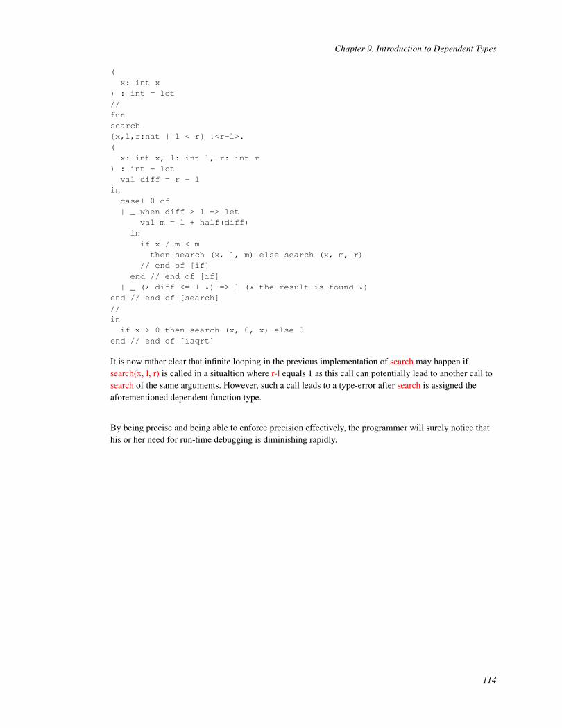
Chapter 9. Introduction to Dependent Types
(x: int x
) : int = let//funsearch{x,l,r:nat | l < r} .<r-l>.(x: int x, l: int l, r: int r
) : int = letval diff = r - l
incase+ 0 of| _ when diff > 1 => let
val m = l + half(diff)inif x / m < mthen search (x, l, m) else search (x, m, r)
// end of [if]end // end of [if]
| _ (* diff <= 1 *) => l (* the result is found *)end // end of [search]//inif x > 0 then search (x, 0, x) else 0
end // end of [isqrt]
It is now rather clear that infinite looping in the previous implementation of search may happen ifsearch(x, l, r) is called in a situaltion where r-l equals 1 as this call can potentially lead to another call tosearch of the same arguments. However, such a call leads to a type-error after search is assigned theaforementioned dependent function type.
By being precise and being able to enforce precision effectively, the programmer will surely notice thathis or her need for run-time debugging is diminishing rapidly.
114

Chapter 10. Datatype Refinement
The datatype mechanism in ATS is adopted from ML directly, and it is really a signatory feature infunctional programming. However, the datatypes we have seen so far are not very precise when employedto classify values. For instance, given a type T, the type list0(T) is for values representing both empty andnon-empty lists consisting of elements of the type T. Therefore, empty and non-empty lists cannot bedistinguished at the level of types. This limitation severely diminishes the effectiveness of datatypes ofML-style in capturing program invariants. In ATS, datatypes of ML-style can be refined into dependentdatatypes of DML-style, where DML refers to the programming language Dependent ML, the immediateprecursor of ATS. With such refinement, datatypes can classify values with greatly enhanced precision.
The code employed for illustration in this chapter plus some additional code for testing is availableon-line (https://github.com/ats-lang/ats-lang.github.io/blob/master/DOCUMENT/INT2PROGINATS/CODE/CHAP_DEPDTREF/).
10.1. Dependent Datatypes
The syntax for declaring dependent datatypes is mostly similar to the syntax for declaring non-dependentdatatypes: For instance, the dependent datatype list in ATS is declared as follows:
datatypelist(t@ype+, int) =| {a:t@ype} list_nil(a, 0) of () // [of ()] is optional| {a:t@ype} {n:nat} list_cons(a, n+1) of (a, list(a, n))
More precisely, list is declared as a type constructor of the sort (t@ype, int) -> type, which means thatlist takes an unboxed type and a static integer to form a boxed type. The keyword t@ype+ indicates thatlist is covariant at its first parameter (of the sort t@ype), that is, list(T1, I) is considered a subtype oflist(T2, I) if T1 is a subtype of T2. There is also the keyword t@ype- for indicating the declared typeconstructor being contravariant at a parameter, but it is rarely used in practice. Also, keywords like type+and type- are interpreted similarly.
There two data (or value) constructors list_nil and list_cons associated with list, which are declared to beof the following types:
list_nil : {a:t@ype} () -> list(a, 0)list_cons : {a:t@ype}{n:nat} (a, list(a, n)) -> list(a, n+1)
Given a type T and a static integer I, the type list(T, I) is for values representing lists of length I in whicheach element is of the type T. Hence, the types of list_nil and list_cons mean that list_nil forms a list oflength 0 and list_cons forms a list of length n+1 if applied to an element and a list of length n. Note thatit is also possible to declare list as follows in a more concise style:
datatype
115

Chapter 10. Datatype Refinement
list (a:t@ype+, int) =| list_nil(a, 0) of () // [of ()] is optional| {n:nat} list_cons(a, n+1) of (a, list(a, n))
The use of a:t@ype+ (instead of t@ype+) introduces implicitly a universal quantifier over a for the typeassigned to each data constructor associated with the declared type constructor list.
As an example of programming with dependent datatypes, the following code implements a functiontemplate for computing the length of a given list:
fun{a:t@ype} list_length{n:nat} .<n>.// .<n>. is a termination metric(xs: list (a, n)): int (n) = case+ xs of| list_nil((*void*)) => 0| list_cons(_(*x*), xs1) => 1 + list_length<a>(xs1)
// end of [list_length]
The type assigned to the function list_length indicates that the function takes a list of length n for anynatural number n and returns an integer of value n. In addition, the function is verified to be terminating.Therefore, list_length is guaranteed to implement the function that computes the length of a given list. Inow briefly explain how typechecking can be performed on the definition of list_length. Let us first seethat the the following clause typechecks:
| list_cons (_, xs1) => 1 + list_length (xs1)
What we need to verify is that the expression on the righthand side of the symbol => can be assigned thetype int(n) under the assumption that xs matches the pattern on the lefthand side of the symbol =>. Let usassume that xs1 is of the type list(a, n1) for some natural number n1, and this assumption implies that thepattern list_cons(_, xs1) is of the type list(a, n1+1). Clearly, matching xs against the pattern list_cons(_,xs1) generates a condition n=n1+1. It is also clear that list_length(xs1) is of the type int(n1) and thus 1 +list_length(xs1) is of the type int(1+n1). As the condition n=n1+1 implies n=1+n1, 1 + list_length(xs1)can be given the type int(n). So this clause typechecks. Note that matching xs against the patternlist_nil() generates the assumption n=0, which implies that 0 is of the type int(n). Therefore, thefollowing clause typechecks:
| list_nil((*void*)) => 0
Given that the two clauses typecheck properly, the case-expression containing them can be assigned thetype int(n). Therefore, the definition of list_length typechecks.
As the recursive call in the body of the above defined function list_length is not a tail-call, the functionmay not be able to handle a long list (e.g., one that contains 1 million elements). The following codegives another implementation for computing the length of a given list:
fun{
116

Chapter 10. Datatype Refinement
a:t@ype} list_length{n:nat} .<>.(xs: list (a, n)): int (n) = let// loop: {i,j:nat} (list (a, i), int (j)) -> int (i+j)fun loop {i,j:nat} .<i>.// .<i>. is a termination metric(xs: list (a, i), j: int j): int (i+j) = case+ xs of| list_cons (_, xs1) => loop (xs1, j+1) | list_nil () => j
// end of [loop]inloop (xs, 0)
end // end of [list_length]
This time, list_length is based on a tail-recursive function loop and thus can handle lists of any length inconstant stack space. Note that the type assigned to loop indicates that loop takes a list of length i and aninteger of value j for some natural numbers i and j and returns an integer of value i+j. Also, loop isverified to be terminating.
There is also a dependent datatype option in ATS for forming optional values:
datatypeoption(a:t@ype+, bool) =| Some (a, true) of a | None (a, false) of ()
// end of [option]
As an example, the following function template list_last tries to find the last element in a given list:
fun{a:t@ype} list_last{n:nat} .<>.
(xs: list (a, n)
) : option (a, n > 0) = let//fun loop{n:pos} .<n>.
(xs: list (a, n)
) : a = letval+ list_cons (_, xs1) = xs
incase+ xs1 of| list_cons _ => loop (xs1)| list_nil () => let
val+ list_cons (x, _) = xs in xend // end of [list_nil]
end // end of [loop]//in
117

Chapter 10. Datatype Refinement
case+ xs of| list_cons _ => Some (loop (xs)) | list_nil () => None ()
end // end of [list_last]
The inner function loop is evidently tail-recursive and it is verified to be terminating.
After a programmer becomes familar with list and option, there is little incentive for him or her to uselist0 and option0 anymore. Internally, values of list and list0 have exactly the same representation andthere are cast functions of zero run-time cost in ATS for translating between values of list and list0. Thesame applies to values of option and option0 as well.
10.2. Example: Function Templates on Lists (Redux)
I have presented previously implementation of some commonly used function templates on lists formedwith the constructors list0_nil and list0_cons. This time, I present as follows implementation of thecorresponding function templates on lists formed with the constructors list_nil and list_cons, whichmake it possible to assign more accurate types to these templates.
Please find the entire code in this section plus some additional code for testing on-line(https://github.com/ats-lang/ats-lang.github.io/blob/master/DOCUMENT/INT2PROGINATS/CODE/CHAP_DEPDTREF/listfuns.dats).
10.2.1. Appending: list_append
Given two lists xs and ys of the types list(T, I1) and list(T, I2) for some type T and integers I1 and I2,list_append(xs, ys) returns a list of the type list(T,I1+I2) that is the concatenation of xs and ys:
fun{a:t@ype} list_append{m,n:nat} .<m>.
(xs: list (a, m), ys: list(a, n)
) : list (a, m+n) =(case+ xs of| list_nil() => ys| list_cons(x, xs) => list_cons(x, list_append<a>(xs, ys))
) (* end of [list_append] *)
Clearly, this implementation of list_append is not tail-recursive.
118

Chapter 10. Datatype Refinement
10.2.2. Reverse Appending: list_reverse_append
Given two lists xs and ys of the type list(T, I1) and list(T, I2) for some type T and integers I1 and I2,list_reverse_append(xs, ys) returns a list of the type list(T, I1+I2) that is the concatenation of the reverseof xs and ys:
fun{a:t@ype} list_reverse_append{m,n:nat} .<m>.
(xs: list(a, m)
, ys: list(a, n)) : list(a, m+n) =(case+ xs of| list_nil () => ys| list_cons (x, xs) =>
list_reverse_append<a>(xs, list_cons(x, ys))) (* end of [list_reverse_append] *)
Clearly, this implementation of list_reverse_append is tail-recursive.
10.2.3. Reversing: list_reverse
Given a list xs, list_reverse(xs) returns the reverse of xs, which is of the same length as xs:
fun{a:t@ype}list_reverse{n:nat} .<>. // defined non-recursively(xs: list(a, n)): list(a, n) = list_reverse_append<a>(xs, list_nil())
// end of [list_reverse]
10.2.4. Mapping: list_map
Given a list xs of the type list(T1, I) for some type T1 and integer I and a closure function f of the typeT1 -<cloref1> T2 for some T2, list_map(xs) returns a list ys of the type list(T2, I):
fun{a:t@ype}{b:t@ype} list_map{n:nat} .<n>.
(xs: list (a, n), f: a -<cloref1> b
) : list (b, n) =
119

Chapter 10. Datatype Refinement
(case+ xs of| list_nil() => list_nil()| list_cons(x, xs) => list_cons(f x, list_map<a>(xs, f))
) (* end of [list_map] *)
Each element y in ys equals f(x), where x is the corresponding element in xs. Clearly, thisimplementation of list_map is not tail-recursive.
10.2.5. Zipping: list_zip
Given two lists xs and ys of the types list(T1, I) and list(T2, I) for some types T1 and T2 and integer I,respectively, list_zip(xs, ys) returns a list zs of the type list((T1,T2), I).
fun{a,b:t@ype} list_zip{n:nat} .<n>.
(xs: list (a, n), ys: list (b, n)
) : list ((a, b), n) =(case+ (xs, ys) of| (
list_nil(), list_nil()) => list_nil((*void*))
| (list_cons (x, xs)
, list_cons (y, ys)) => list_cons((x, y), list_zip<a,b>(xs, ys))
) (* end of [list_zip] *)
Each element z in zs equals the pair (x, y), where x and y are the corresponding elements in xs and ys,respectively. Clearly, this implementation of list_zip is not tail-recursive.
10.2.6. Zipping with: list_zipwith
Given two lists xs and ys of the types list(T1, I) and list(T2, I) for some types T1 and T2 and integer I,respectively, and a closure function f of the type (T1, T2) -<cloref1> T3 for some type T3,list_zipwith(xs, ys, f) returns a list zs of the type list(T3, I):
fun{a,b:t@ype}{c:t@ype} list_zipwith{n:nat} .<n>.
(
120

Chapter 10. Datatype Refinement
xs: list (a, n), ys: list (b, n), f: (a, b) -<cloref1> c) : list (c, n) =(case+ (xs, ys) of| (
list_nil(), list_nil()) => list_nil((*void*))
| (list_cons(x, xs)
, list_cons(y, ys)) =>list_cons(f(x, y), list_zipwith<a,b><c>(xs, ys, f))
// end of (list_cons, list_cons)) (* end of [list_zipwith] *)
Each element z in zs equals f(x, y), where x and y are the corresponding elements in xs and ys,respectively. Clearly, this implementation of list_zipwith is not tail-recursive.
10.3. Example: Mergesort on Lists (Redux)
I have previously presented an implementation of mergesort on lists that are formed with the constructorslist0_nil and list0_cons. In this section, I give an implementation of mergesort on lists formed with theconstructors list_nil and list_cons. This implementation is based on the same algorithm as the previousone but it assigns a type to the implemented sorting function that guarantees the function to belength-preserving, that is, the function always returns a list of the same length as the list it sorts.
The following defined function merge combines two ordered list (according to a given ordering) into asingle ordered list:
//typedef lte (a:t@ype) = (a, a) -> bool//fun{a:t@ype} merge{m,n:nat} .<m+n>.
(xs0: list (a, m), ys0: list (a, n), lte: lte a
) : list (a, m+n) =case+ xs0 of| list_nil() => ys0| list_cons(x, xs1) =>(case+ ys0 of| list_nil() => xs0
121

Chapter 10. Datatype Refinement
| list_cons(y, ys1) =>if x \lte ythen list_cons (x, merge (xs1, ys0, lte))else list_cons (y, merge (xs0, ys1, lte))
// end of [if]) // end of [list_cons]
// end of [merge]//
Clearly, the type assigned to merge indicates that the function returns a list whose length equals the sumof the lengths of the two input lists. Note that a termination metric is present for verifying that merge is aterminating function.
The following defined function mergesort mergesorts a list according to a given ordering:
fun{a:t@ype} mergesort{n:nat}(xs: list (a, n), lte: lte a
) : list (a, n) = let//fun msort{n:nat} .<n,n>.
(xs: list (a, n), n: int n, lte: lte a
) : list (a, n) =if n >= 2then split (xs, n, lte, half(n), list_nil) else xs
// end of [if]// end of [msort]and split{n:int | n >= 2}{i:nat | i <= n/2} .<n,i>.
(xs: list (a, n-n/2+i)
, n: int n, lte: lte a, i: int i, xsf: list (a, n/2-i)) : list (a, n) =if i > 0 then letval+ list_cons (x, xs) = xs
insplit (xs, n, lte, i-1, list_cons (x, xsf))
end else letval n2 = half(n)val xsf = list_reverse<a> (xsf) // make sorting stable!val xsf = list_of_list_vt (xsf) // linear list -> nonlinear listval xsf = msort (xsf, n2, lte) and xs = msort (xs, n-n2, lte)
inmerge (xsf, xs, lte)
end // end of [if]// end of [split]
//in
122

Chapter 10. Datatype Refinement
msort(xs, list_length<a>(xs), lte)end // end of [mergesort]
The type assigned to mergesort indicates that mergesort returns a list of the same length as its input list.The two inner functions msort and split are defined mutually recursively, and the termination metrics forthem are pairs of natural numbers that are compared according to the standard lexicographic ordering oninteger sequences. The type assigned to msort clearly indicates that its integer argument is required to bethe length of its list argument, and a mismatch between the two surely results in a type-error. The typeassigned to split is particularly informative, depicting a relation between the arguments and the returnvalue of the function that can be of great help for someone trying to understand the code. The functionlist_reverse returns a linear list that is the reverse of its input, and the cast function list_of_list_vt turns alinear list into a nonlinear one (while incuring no cost at run-time). I will explain what linear lists areelsewhere.
Please find the entire code in this section plus some additional code for testing on-line(https://github.com/ats-lang/ats-lang.github.io/blob/master/DOCUMENT/INT2PROGINATS/CODE/CHAP_DEPDTREF/mergesort.dats).
10.4. Sequentiality of Pattern Matching
In ATS, pattern matching is performed sequentially at run-time. In other words, a clause is selected onlyif a given value matches the pattern guard associated with this clause but the value fails to match thepattern associated with any clause ahead of it. Naturally, one may expect that the followingimplementation of list_zipwith also typechecks:
fun{a,b:t@ype}{c:t@ype} list_zipwith{n:nat}
(xs: list(a, n)
, ys: list(b, n), f: (a, b) -<cloref1> c) : list(c, n) = (//case+ (xs, ys) of| (
list_cons(x, xs), list_cons(y, ys)) =>(list_cons(f(x, y), list_zipwith<a,b><c>(xs, ys, f))
)| (_, _) => list_nil((*void*))//) (* end of [list_zipwith] *)
123

Chapter 10. Datatype Refinement
This, however, is not the case. In ATS, typechecking clauses is done nondeterministically (rather thansequentially). In this example, the second clause fails to typecheck as it is done without the assumptionof the given pair (xs, ys) failing to match the pattern guard associated with the first clause. The secondclause can be modified slightly as follows to pass typechecking:
| (_, _) =>> list_nil((*void*))
The use of the symbol =>> (in place of =>) indicates to the typechecker that this clause needs to betypechecked under the sequentiality assumption that the given value matching it does not match thepattern guards associated with any previous clauses. Therefore, when the modified second clause istypechecked, it can be assumed that the pair (xs, ys) matching the pattern (_, _) must match one of thefollowing three patterns:
• (list_cons _, list_nil ())
• (list_nil (), list_cons _)
• (list_nil (), list_nil ())
Given that xs and ys are of the same length, the typechecker can readily infer that (xs, ys) cannot matcheither of the first two patterns. After these two patterns are ruled out, typechecking is essentially done asif the second clause was written as follows:
| (list_nil(), list_nil()) => list_nil((*void*))
One may be wondering why typechecking clauses is not required to be done sequentially by default. Thesimple reason is that this requirement, if fully enforced, can have a great negative impact on the efficiencyof typechecking. Therefore, it is a reasonable design to provide the programmer with an explict means tooccasionally make use of the sequentiality assumption needed for typechecking a particular clause.
10.5. Example: Functional Red-Black Trees
A red-black tree is defined as a binary tree such that each node in it is colored red or black and every pathfrom the root to a leaf has the same number of black nodes while containing no occurrences of two rednodes in a row. Clearly, the length of a longest path in each red-black tree is bounded by 2 times thelength of a shortest path in it. Therefore, red-black trees are a family of balanced trees. The number ofblack nodes occurring on each path in a red-black tree is often referred to as the black height of the tree.
Formally, a datatype precisely for red-black trees can be declared in ATS as follows:
//#define BLK 0#define RED 1sortdef clr = {c:nat | c <= 1}
124

Chapter 10. Datatype Refinement
//datatype rbtree(a:t@ype+, int(*clr*), int(*bh*)) =| rbtree_nil (a, BLK, 0)| {c,cl,cr:clr | cl <= 1-c; cr <= 1-c} {bh:nat}rbtree_cons (a, c, bh+1-c) of (int c, rbtree (a, cl, bh), a, rbtree (a, cr, bh))
// end of [rbtree]//
The color of a tree is the color of its root node or is black if the tree is empty. Given a type T, a color C(represented by a integer) and an integer BH, the type rbtree(T, C, BH) is for red-black trees carryingelements of the type T that is of the color C and the black height BH.
When implementing various operations (such as insertion and deletion) on a red-black tree, we oftenneed to first construct intermediate trees that contain color violations caused by a red node beingfollowed by another red node and then employ tree rotations to fix such violations. This need makes theabove datatype rbtree too rigid as it cannot be assigned to any intermediate trees containing colorviolations. To address this issue, we can declare rbtree as follows:
//datatype rbtree(a:t@ype+
, int // color, int // black height, int // violations) = // rbtree| rbtree_nil (a, BLK, 0, 0) of ()| {c,cl,cr:clr}{bh:nat}{v:int}
{c==BLK && v==0 || c == RED && v==cl+cr}rbtree_cons (a, c, bh+1-c, v) of(int c, rbtree0 (a, cl, bh), a, rbtree0(a, cr, bh)
) (* end of [rbtree_cons] *)// end of [rbtree]//where rbtree0(a:t@ype, c:int, bh:int) = rbtree(a, c, bh, 0)//
We count each occurrence of two red nodes in a row as one color violation. Given a type T, a color C(represented by a integer), an integer BH and an integer V, the type rbtree(T, C, BH, V) is for treescarrying elements of the type T that is of the color C and the black height BH and contains exactly Vcolor violations. Therefore, the type rbtree(T, C, BH, 0) is for valid red-black trees (containing no colorviolations).
Given a tree containing at most one color violation, an element and another tree containing no violations,the following operation constructs a valid red-black tree:
fn{
125

Chapter 10. Datatype Refinement
a:t@ype} insfix_l // right rotation for fixing left insertion{cl,cr:clr} {bh:nat} {v:nat} (tl: rbtree (a, cl, bh, v), x0: a, tr: rbtree (a, cr, bh, 0)
) : [c:clr] rbtree0 (a, c, bh+1) = let#define B BLK; #define R RED; #define cons rbtree_cons
incase+ (tl, x0, tr) of| (cons (R, cons (R, a, x, b), y, c), z, d) =>
cons (R, cons (B, a, x, b), y, cons (B, c, z, d)) // shallow rot| (cons (R, a, x, cons (R, b, y, c)), z, d) =>
cons (R, cons (B, a, x, b), y, cons (B, c, z, d)) // deep rotation| (a, x, b) =>> cons (B, a, x, b)
end // end of [insfix_l]
By simply reading the interface of insfix_l, we can see that the two tree arguments are required to be ofthe same black height bh for some natural number bh and the returned tree is of the black height bh+1.
The following operation insfix_r is just the mirror image of insfix_l:
fn{a:t@ype} insfix_r // left rotation for fixing right insertion{cl,cr:clr} {bh:nat} {v:nat} (tl: rbtree (a, cl, bh, 0), x0: a, tr: rbtree (a, cr, bh, v)
) : [c:clr] rbtree0 (a, c, bh+1) = let#define B BLK; #define R RED; #define cons rbtree_cons
incase+ (tl, x0, tr) of| (a, x, cons (R, b, y, cons (R, c, z, d))) =>
cons (R, cons (B, a, x, b), y, cons (B, c, z, d)) // shallow rot| (a, x, cons (R, cons (R, b, y, c), z, d)) =>
cons (R, cons (B, a, x, b), y, cons (B, c, z, d)) // deep rotation| (a, x, b) =>> cons (B, a, x, b)
end // end of [insfix_r]
The preparation for implementing insertion on a red-black tree is all done by now, and we are ready tosee an implementation of insertion guaranteeing that the tree obtained from inserting an element into agiven red-black tree is always a valid red-black tree itself. This guarantee is precisely captured in thefollowing interface for insertion:
externfun{a:t@ype} rbtree_insert{c:clr} {bh:nat}
(t: rbtree0 (a, c, bh), x0: a, cmp: cmp a
) : [bh1:nat] rbtree0 (a, BLK, bh1)
126

Chapter 10. Datatype Refinement
Interestingly, this interface also implies that the tree returned by a call to rbtree_insert is always black.The code presented below gives an implementation of rbtree_insert:
implement{a}rbtree_insert(t, x0, cmp) = let
//#define B BLK#define R RED#define nil rbtree_nil#define cons rbtree_cons//fun ins{c:clr}{bh:nat} .<bh,c>.
(t: rbtree0 (a, c, bh), x0: a
) :[cl:clr;v:nat | v <= c
] rbtree (a, cl, bh, v) =(case+ t of| nil ((*void*)) =>
cons{..}{..}{..}{0} (R, nil, x0, nil)| cons (c, tl, x, tr) => let
val sgn = compare (x0, x, cmp)inif sgn < 0 then letval [cl,v:int] tl = ins (tl, x0)
inif c = B then insfix_l (tl, x, tr)else cons{..}{..}{..}{cl} (R, tl, x, tr)
// end of [if]end else if sgn > 0 then letval [cr,v:int] tr = ins (tr, x0)
inif c = B then insfix_r (tl, x, tr)else cons{..}{..}{..}{cr} (R, tl, x, tr)
// end of [if]end else t // end of [if]
end // end of [cons]) (* end of [ins] *)//val t = ins (t, x0)//incase+ t of cons (R, tl, x, tr) => cons (B, tl, x, tr) | _ =>> t
end // end of [rbtree_insert]
Note that the type assigned to the inner function ins is so informative that it literally gives an formalexplanation about the way in which insertion works on a red-black tree. Many a programmer implementsred-black trees by simply following an algorithm written in some format of pseudo code while having
127

Chapter 10. Datatype Refinement
little understanding about the innerworkings of the algorithm. For instance, if the above inner functionins is implemented in C, few programmers are likely to see that the function always maintain the blackheight of a given red-black tree after insertion but may introduce one color violation if the root of the treeis red. On the other hand, knowing this invariant is essential to gaining a thorough understanding of theinsertion algorithm on red-black trees.
The insertion operation implemented above does not insert an element if it is already in the givenred-black tree. It may be desirable to require that the operation inform the caller if such a case occurs.For instance, an exception can be raised for this purpose. An alternative is to give rbtree_insert acall-by-reference argument so that a flag can be returned in it to indicate whether the element to beinserted is actually inserted. I will explain elsewhere what call-by-reference is and how it is supported inATS.
Often deleting an element from a binary search tree is significantly more difficult to implement thaninserting one. This is especially so in the case of a red-black tree. I refer the interested reader to the libatslibrary of ATS for some code implementing a deletion operation on red-black trees that can guaranteebased on types each tree returned by the operation being a valid red-black tree (containing no colorviolations).
Please find the entire code in this section plus some additional code for testing on-line(https://github.com/ats-lang/ats-lang.github.io/blob/master/DOCUMENT/INT2PROGINATS/CODE/CHAP_DEPDTREF/rbtree.dats).
128

Chapter 11. Theorem-Proving in ATS/LF
Within the ATS programming language system, there is a component named ATS/LF for supporting(interactive) therorem-proving. In ATS/LF, theorem-proving is done by constructing proofs as totalfunctional programs. It will soon become clear that this style of theorem-proving can be combinedcohesively with functional programming to yield a programming paradigm that is considered thesignature of ATS: programming with theorem-proving. Moreover, ATS/LF can be employed to encodevarious deduction systems and their meta-properties.
Please find on-line (https://github.com/ats-lang/ats-lang.github.io/blob/master/DOCUMENT/INT2PROGINATS/CODE/CHAP_THMPRVING/) the codeemployed for illustration in this chapter plus some additional code for testing.
11.1. Encoding Relations as Dataprops
In the statics of ATS, there is a built-in sort prop for static terms that represent types for proofs. A staticterm of the sort prop can also be referred to as a type or more accurately, a prop-type or just a prop. Adataprop can be declared in a manner that is mostly similar to the declaration of a datatype. For instance,a prop construct FIB is introduced in the following dataprop declaration:
datapropFIB(int, int) =| FIB0(0, 0) of () // [of ()] can be dropped| FIB1(1, 1) of () // [of ()] can be dropped| {n:nat}{r0,r1:int}FIB2(n+2, r0+r1) of (FIB(n, r0), FIB(n+1, r1))
// end of [FIB]
The sort assigned to FIB is (int, int) -> prop, indicating that FIB takes two static integers to form aprop-type. There are three data (or proof) constructors associated with FIB: FIB0, FIB1 and FIB2, whichare assigned the following function types (or more accurately, prop-types):
• FIB0: () -> FIB(0, 0)
• FIB1: () -> FIB(1, 1)
• FIB2: {n:nat}{r0,r1:int} (FIB(n, r0), FIB(n+1, r1)) -> FIB(n+2, r0+r1)
Given a natural number n and an integer r, it should be clear that FIB(n, r) encodes the relation fib(n) = r,where fib is defined by the following three equations:
• fib(0) = 0, and
• fib(1) = 1, and
• fib(n+2) = fib(n) + fib(n+1) for n >= 2.
129

Chapter 11. Theorem-Proving in ATS/LF
A proof value of the prop FIB(n, r) can be constructed if and only if fib(n) equals r. For instance, theproof value FIB2(FIB0(), FIB1()) is assigned the prop FIB(2, 1), attesting to fib(2) equaling 1.
As another example of dataprop, the following declaration introduces a prop constructor MUL togetherwith three associated proof constructors:
datapropMUL(int, int, int) =| {n:int} MULbas(0, n, 0) of ()| {m:nat}{n:int}{p:int}MULind(m+1, n, p+n) of MUL(m, n, p)
| {m:pos}{n:int}{p:int}MULneg(~(m), n, ~(p)) of MUL(m, n, p)
// end of [MUL]
Given three integers m, n and p, the prop MUL(m, n, p) encodes the relation m*n = p. As for MULbas,MULind and MULneg, they correspond to the following three equations, respectively:
• 0*n = 0 for every integer n, and
• (m+1)*n = m*n + n for each pair of integers m and n, and
• (~m)*n = ~(m*n) for each pair of integers m and n.
In other words, the dataprop declaration for MUL encodes the relation that represents the standardmultiplication function on integers.
It can be readily noticed that the process of encoding a functional relation (i.e., a relation representing afunction) as a dataprop is analogous to implementing a function in a logic programming language suchas Prolog.
11.2. Constructing Proofs as Total Functions
Theorems are represented as types (or more accurately, props) in ATS/LF. For instance, the followingprop states that integer multiplication is commutative:
{m,n:int}{p:int} MUL(m, n, p) -<prf> MUL(n, m, p)
Constructing a proof for a theorem in ATS/LF means implementing a total value (which is most likely tobe a total function) of the type that is the encoding of the theorem in ATS/LF, where being total meansbeing pure and terminating. Please note that this style of theorem-proving may seem rather peculiar tothose who have never tried it before.
As a simple introductory example, let us first construct a proof function in ATS/LF that is given thefollowing interface:
130

Chapter 11. Theorem-Proving in ATS/LF
prfun mul_istot {m,n:int} (): [p:int] MUL(m, n, p)
The keyword prfun indicates that the interface is for a proof function (in contrast to a non-prooffunction). Note that mul_istot is declared to be of the following type (or more accurately, prop):
{m,n:int} () -<prf> [p:int] MUL(m, n, p)
which essentially states that integer multiplication is a total function: Given any two integers m and n,there exists an integer p such that m, n and p are related according to the structurally inductively definedrelation MUL. The following code gives an implementation of mul_istot:
primplementmul_istot{m,n}() = let//prfun istot{m:nat;n:int} .<m>. (): [p:int] MUL(m, n, p) =sif m > 0 then MULind(istot{m-1,n}()) else MULbas()
// end of [istot]//insif m >= 0 then istot{m,n}() else MULneg(istot{~m,n}())
end // end of [mul_istot]
Note that the keyword primplement (instead of implement) initiates the implementation of a proof. Theinner proof function istot encodes a proof showing that there exists an integer p for any given naturalnumber m and integer n such that m, n and p are related (according to MUL). The keyword sif is used forforming a conditional (proof) expression in which the test is a static expression. The proof encoded byistot proceeds by induction on m; if m > 0 holds, then there exists an integer p1 such that m-1, n and p1are related by induction hypothesis (on m-1) and thus m, n and p are related for p = p1+n according tothe rule encoded by MULind; if m = 0, then m, n and p are related for p = 0. The proof encoded by theimplementation of mul_istot goes like this: if m is a natural number, then the lemma proven by istotshows that m, n and some p are related; if m is negative, then the same lemma shows that ~m, n and p1are related for some integer p1 and thus m, n and p are related for p = ~p1 according to the rule encodedby MULneg.
As another example of theorem-proving in ATS/LF, a proof function of the name mul_isfun is given asfollows:
prfn mul_isfun{m,n:int}{p1,p2:int}
(pf1: MUL(m, n, p1), pf2: MUL(m, n, p2)
) : [p1==p2] void = letprfun isfun{m:nat;n:int}{p1,p2:int} .<m>.
(pf1: MUL(m, n, p1), pf2: MUL(m, n, p2)
) : [p1==p2] void =case+ pf1 of
131

Chapter 11. Theorem-Proving in ATS/LF
| MULind(pf1prev) => letprval MULind(pf2prev) = pf2 in isfun (pf1prev, pf2prev)
end // end of [MULind]| MULbas() => let
prval MULbas() = pf2 in ()end // end of [MULbas]
// end of [isfun]incase+ pf1 of| MULneg(pf1nat) => let
prval MULneg(pf2nat) = pf2 in isfun (pf1nat, pf2nat)end // end of [MULneg]
| _ (*non-MULneg*) =>> isfun (pf1, pf2)end // end of [mul_isfun]
The keyword prfn is used for defining a non-recursive proof function, and the keyword prval forintroducing bindings that relate names to proof expressions, that is, expressions of prop-types. As far aspattern matching exhaustiveness is concerned, prval is equivalent to val+ (as proofs cannot contain anyeffects such as failures of pattern matching).
What mul_isfun proves is that the relation MUL is functional on its first two arguments: If m, n and p1are related according to MUL and m, n and p2 are also related according to MUL, then p1 and p2 areequal. The statement is first proven by the inner proof function isfun under the assumption that m is anatural number, and then the assumption is dropped. Let us now take a look at the first matching clausein the body of isfun. If the clause is chosen, then pf1 matches the pattern MULind(pf1prev) and thuspf1prev is of the type MUL(m1, n1, q1) for some natural number m1 and integer n1 and integer p1 suchthat m=m1+1, n=n1, and p1=q1+n1. This means that pf2 must be of the form MULind(pf2prev) for somepf2prev of the type MUL(m2, n2, q2) such that m2+1=m, n2=n and p2=q2+n2. By calling isfun onpf1prev and pf2prev, which amounts to invoking the induction hypothesis on m-1, we establish q1=q2,which implies p1=p2. The second matching clause in the body of isfun can be readily understood, whichcorresponds to the base case in the inductive proof encoded by isfun.
11.3. Example: Distributivity of Multiplication
The distributivity of multiplication over addition means that the following equation holds
m * (n1 + n2) = m * n1 + m * n2
for m, n1 and n2 ranging over integers. A direct encoding of the equation is given by the following(proof) function interface:
//prfunmul_distribute{m,n1,n2:int}{p1,p2:int}(MUL(m, n1, p1), MUL(m, n2, p2)): MUL(m, n1+n2, p1+p2)
//
132

Chapter 11. Theorem-Proving in ATS/LF
Plainly speaking, the encoding states that the product of m and (n1+n2) is p1+p2 if the product of m andn1 is p1 and the product of m and n2 is p2. An implementation of mul_distribute is given as follows:
primplementmul_distribute{m,n1,n2}{p1,p2}(pf1, pf2) = let
//prfunauxnat{m:nat}{p1,p2:int} .<m>.(pf1: MUL(m, n1, p1), pf2: MUL(m, n2, p2)
) : MUL(m, n1+n2, p1+p2) =(case+ (pf1, pf2) of| (MULbas(), MULbas()) => MULbas()| (MULind pf1, MULind pf2) => MULind(auxnat (pf1, pf2))
) (* end of [auxnat] *)//in//sifm >= 0then (auxnat (pf1, pf2)
) // end of [then]else letprval MULneg(pf1) = pf1prval MULneg(pf2) = pf2
inMULneg(auxnat (pf1, pf2))
end // end of [else]//end // end of [mul_distribute]
The inner function auxnat encodes a straighforward proof based on mathematical induction thatestablishes the following equation:
m * (n1 + n2) = m * n1 + m * n2
for m ranging over natural numbers and n1 and n2 ranging over integers. The function mul_distribute canthen be implemented immediately based on auxnat.
133

Chapter 11. Theorem-Proving in ATS/LF
11.4. Example: Commutativity of Multiplication
The commutativity of multiplication means that the following equation holds
m * n = n * m
for m and n ranging over integers. A direct encoding of this equation is given by the following (proof)function interface:
//prfunmul_commute{m,n:int}{p:int}(MUL(m, n, p)): MUL(n, m, p)//
An implementation of mul_commute is given as follows:
primplmntmul_commute{m,n}{p}(pf0) = let
//prfunauxnat{m:nat}{p:int} .<m>.(pf: MUL(m, n, p)) : MUL(n, m, p) =(case+ pf of| MULbas() => mul_nx0_0{n}()| MULind(pf1) =>
mul_distribute(auxnat(pf1), mul_nx1_n{n}())// end of [MULind]
) (* end of [auxnat] *)//in//sifm >= 0then auxnat(pf0)else letprval MULneg(pf1) = pf0 in mul_neg_2(auxnat(pf1))
end // end of [else]//end // end of [mul_commute]
where the following proof functions are called:
//prfun
134
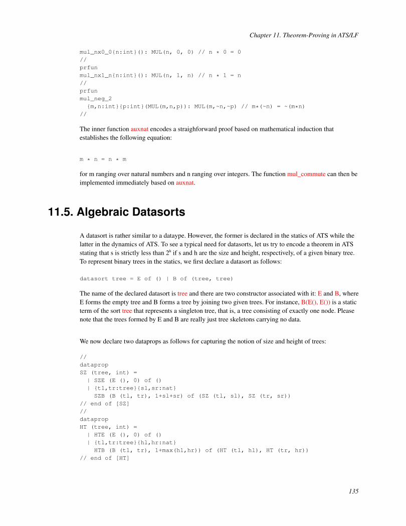
Chapter 11. Theorem-Proving in ATS/LF
mul_nx0_0{n:int}(): MUL(n, 0, 0) // n * 0 = 0//prfunmul_nx1_n{n:int}(): MUL(n, 1, n) // n * 1 = n//prfunmul_neg_2{m,n:int}{p:int}(MUL(m,n,p)): MUL(m,~n,~p) // m*(~n) = ~(m*n)
//
The inner function auxnat encodes a straighforward proof based on mathematical induction thatestablishes the following equation:
m * n = n * m
for m ranging over natural numbers and n ranging over integers. The function mul_commute can then beimplemented immediately based on auxnat.
11.5. Algebraic Datasorts
A datasort is rather similar to a dataype. However, the former is declared in the statics of ATS while thelatter in the dynamics of ATS. To see a typical need for datasorts, let us try to encode a theorem in ATSstating that s is strictly less than 2h if s and h are the size and height, respectively, of a given binary tree.To represent binary trees in the statics, we first declare a datasort as follows:
datasort tree = E of () | B of (tree, tree)
The name of the declared datasort is tree and there are two constructor associated with it: E and B, whereE forms the empty tree and B forms a tree by joining two given trees. For instance, B(E(), E()) is a staticterm of the sort tree that represents a singleton tree, that is, a tree consisting of exactly one node. Pleasenote that the trees formed by E and B are really just tree skeletons carrying no data.
We now declare two dataprops as follows for capturing the notion of size and height of trees:
//datapropSZ (tree, int) =| SZE (E (), 0) of ()| {tl,tr:tree}{sl,sr:nat}SZB (B (tl, tr), 1+sl+sr) of (SZ (tl, sl), SZ (tr, sr))
// end of [SZ]//datapropHT (tree, int) =| HTE (E (), 0) of ()| {tl,tr:tree}{hl,hr:nat}HTB (B (tl, tr), 1+max(hl,hr)) of (HT (tl, hl), HT (tr, hr))
// end of [HT]
135

Chapter 11. Theorem-Proving in ATS/LF
//
Given a tree t and an integer s, SZ(t, s) encodes the relation that the size of t equals s. Similiarly, given atree t and an integer h, HZ(t, h) encodes the relation that the height of t equals h.
As the power function (of base 2) is not available in the statics of ATS, we declare a dataprop as followsto capture it:
datapropPOW2 (int, int) =| POW2bas (0, 1)| {n:nat}{p:int} POW2ind (n+1, p+p) of POW2 (n, p)
// end of [POW2]
Given two integers h and p, POW2 (h, p) encodes the relation that 2h equals p.
It should be clear by now that the following proof function interface encodes the theorem stating that s isstrictly less than 2h if s and h are the size and height of a given binary tree:
prfunlemma_tree_size_height{t:tree}{s,h:nat}{p:int}
(pf1: SZ (t, s), pf2: HT (t, h), pf3: POW2 (h, p)
) : [s < p] void // end of [prfun]
Let us now construct an implementation of this proof function as follows.
We first establish some elementary properties on the power function (of base 2):
prfunpow2_istot{h:nat} .<h>. (): [p:int] POW2 (h, p) =sif h==0then POW2bas () else POW2ind (pow2_istot {h-1} ())
// end of [sif]// end of [pow2_istot]
prfunpow2_pos{h:nat}{p:int} .<h>.(pf: POW2 (h, p)): [p > 0] void =case+ pf of| POW2bas () => () | POW2ind (pf1) => pow2_pos (pf1)
// end of [pow2_pos]
prfunpow2_inc{h1,h2:nat | h1 <= h2}{p1,p2:int} .<h2>.(pf1: POW2 (h1, p1), pf2: POW2 (h2, p2)): [p1 <= p2] void =
136

Chapter 11. Theorem-Proving in ATS/LF
case+ pf1 of| POW2bas () => pow2_pos (pf2)| POW2ind (pf11) => let
prval POW2ind (pf21) = pf2 in pow2_inc (pf11, pf21)end // end of [POW2ind]
// end of [pow2_inc]
Clearly, pow2_istot shows that the relation encoded by the dataprop POW2 is a total relation; pow2_posproves that the power of each natural number is positive; pow2_inc establishes that the power function isincreasing.
The function lemma_tree_size_height can be implemented as follows:
primplementlemma_tree_size_height(pf1, pf2, pf3) = let
//prfunlemma{t:tree}{s,h:nat}{p:int} .<t>.
(pf1: SZ (t, s)
, pf2: HT (t, h), pf3: POW2 (h, p)) : [p > s] void =(scase t of| E () => let
prval SZE () = pf1prval HTE () = pf2prval POW2bas () = pf3
in// nothing
end // end of [E]| B (tl, tr) => let
prval SZB (pf1l, pf1r) = pf1prval HTB {tl,tr}{hl,hr} (pf2l, pf2r) = pf2prval POW2ind (pf31) = pf3prval pf3l = pow2_istot {hl} ()prval pf3r = pow2_istot {hr} ()prval () = lemma (pf1l, pf2l, pf3l)prval () = lemma (pf1r, pf2r, pf3r)prval () = pow2_inc (pf3l, pf31)prval () = pow2_inc (pf3r, pf31)
in// nothing
end // end of [B]) (* end of [lemma] *)//inlemma (pf1, pf2, pf3)
end // end of [lemma_tree_size_height]
137
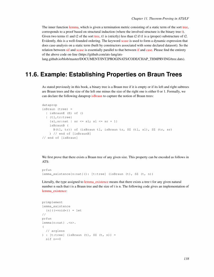
Chapter 11. Theorem-Proving in ATS/LF
The inner function lemma, which is given a termination metric consisting of a static term of the sort tree,corresponds to a proof based on structural induction (where the involved structure is the binary tree t).Given two terms t1 and t2 of the sort tree, t1 is (strictly) less than t2 if t1 is a (proper) substructure of t2.Evidently, this is a well-founded ordering. The keyword scase is used to form a dynamic expression thatdoes case-analysis on a static term (built by constructors associated with some declared datasort). So therelation between sif and scase is essentially parallel to that between if and case. Please find the entiretyof the above code on-line (https://github.com/ats-lang/ats-lang.github.io/blob/master/DOCUMENT/INT2PROGINATS/CODE/CHAP_THMPRVING/tree.dats).
11.6. Example: Establishing Properties on Braun Trees
As stated previously in this book, a binary tree is a Braun tree if it is empty or if its left and right subtreesare Braun trees and the size of the left one minus the size of the right one is either 0 or 1. Formally, wecan declare the following dataprop isBraun to capture the notion of Braun trees:
datapropisBraun (tree) =| isBraunE (E) of ()| {tl,tr:tree}{sl,sr:nat | sr <= sl; sl <= sr + 1}isBraunB (B(tl, tr)) of (isBraun tl, isBraun tr, SZ (tl, sl), SZ (tr, sr)
) // end of [isBraunB]// end of [isBraun]
We first prove that there exists a Braun tree of any given size. This property can be encoded as follows inATS:
prfunlemma_existence{n:nat}(): [t:tree] (isBraun (t), SZ (t, n))
Literally, the type assigned to lemma_existence means that there exists a tree t for any given naturalnumber n such that t is a Braun tree and the size of t is n. The following code gives an implementation oflemma_existence:
primplementlemma_existence{n}((*void*)) = let
//prfunlemma{n:nat} .<n>.(// argless
) : [t:tree] (isBraun (t), SZ (t, n)) =sif n==0
138

Chapter 11. Theorem-Proving in ATS/LF
then (isBraunE (), SZE ())else letstadef nl = n / 2stadef nr = n - 1 - nlval (pfl1, pfl2) = lemma{nl}((*void*))and (pfr1, pfr2) = lemma{nr}((*void*))
in(isBraunB (pfl1, pfr1, pfl2, pfr2), SZB (pfl2, pfr2))
end // end of [else]// end of [sif]
//inlemma{n}((*void*))
end // end of [lemma_existence]
Note that stadef is a keyword in ATS for introducting a static binding between a name and a static term(of any sort). If one prefers, this keyword can be chosen to replace the keyword typedef (for introducinga name and a static term of the sort t@ype).
Next we show that two Braun trees of the same size are identical. This property can be encoded asfollows:
prfunlemma_unicity{n:nat}{t1,t2:tree}
(pf1: isBraun t1, pf2: isBraun t2, pf3: SZ (t1, n), pf4: SZ (t2, n)
) : EQ (t1, t2) // end of [lemma_unicity]
where EQ is a prop-constructor introduced by the following dataprop declaration:
dataprop EQ (tree, tree) =| EQE (E, E) of ()| {t1l,t1r:tree}{t2l,t2r:tree}EQB (B (t1l, t1r), B (t2l, t2r)) of (EQ (t1l, t2l), EQ (t1r, t2r))
// end of [EQ]
Clearly, EQ is the inductively defined equality on trees. An implementation of the proof functionlemma_unicity is presented as follows:
primplementlemma_unicity(pf1, pf2, pf3, pf4) = letprfun lemma{n:nat}{t1,t2:tree} .<n>.(pf1: isBraun t1, pf2: isBraun t2, pf3: SZ (t1, n), pf4: SZ (t2, n)
) : EQ (t1, t2) =sif n==0then letprval SZE () = pf3 and SZE () = pf4
139

Chapter 11. Theorem-Proving in ATS/LF
prval isBraunE () = pf1 and isBraunE () = pf2inEQE ()
end // end of [then]else letprval SZB (pf3l, pf3r) = pf3prval SZB (pf4l, pf4r) = pf4prval isBraunB (pf1l, pf1r, pf1lsz, pf1rsz) = pf1prval isBraunB (pf2l, pf2r, pf2lsz, pf2rsz) = pf2prval () = SZ_istot (pf1lsz, pf3l) and () = SZ_istot (pf1rsz, pf3r)prval () = SZ_istot (pf2lsz, pf4l) and () = SZ_istot (pf2rsz, pf4r)prval pfeql = lemma (pf1l, pf2l, pf3l, pf4l)prval pfeqr = lemma (pf1r, pf2r, pf3r, pf4r)
inEQB (pfeql, pfeqr)
end // end of [else]// end of [sif]
inlemma (pf1, pf2, pf3, pf4)
end // end of [lemma_unicity]
Note that the proof function SZ_istot in this implementation of lemma_unicity is given the followinginterface:
prfunSZ_istot{t:tree}{n1,n2:int}(pf1: SZ (t, n1), pf2: SZ (t, n2)): [n1==n2] void
which simply states that SZ is a functional relation with respect to its first parameter, that is, there is atmost one n for every given t such that t and n are related according to SZ. Clearly, the mathematicalproof corresponding to this implementation is of induction on the size n of the two given trees t1 and t2.In the base case where n is 0, t1 and t2 are equal as they both are the empty tree. In the inductive casewhere n > 0, it is proven that n1l and n2l are of the same value where n1l and n2l are the sizes of the leftsubtrees of t1 and t2, respecitvely; similarly, it is also proven that n1r and n2r are of the same valuewhere n1r and n2r are the sizes of the right subtrees of t1 and t2, respectively; by induction hypothesis onn1l, the left substrees of t1 and t2 are the same; by induction hypothesis on n1r, the right substrees of t1and t2 are the same; by the definition of tree equality (encoded by EQ), t1 and t2 are the same.
As a comparison, the following code gives another implementation of lemma_unicity that is of adifferent (and rather unusual) style:
primplementlemma_unicity(pf1, pf2, pf3, pf4) = let
//prfunlemma{n:nat}{t1,t2:tree} .<t1>.(pf1: isBraun t1, pf2: isBraun t2, pf3: SZ (t1, n), pf4: SZ (t2, n)
) : EQ (t1, t2) =
140

Chapter 11. Theorem-Proving in ATS/LF
case+ (pf1, pf2) of//| (isBraunE (), isBraunE ()) => EQE ()
//| (isBraunB (pf11, pf12, pf13, pf14),
isBraunB (pf21, pf22, pf23, pf24)) => let//
prval SZB (pf31, pf32) = pf3prval SZB (pf41, pf42) = pf4
//prval () = SZ_istot (pf13, pf31)prval () = SZ_istot (pf23, pf41)
//prval () = SZ_istot (pf14, pf32)prval () = SZ_istot (pf24, pf42)
//prval pfeq1 = lemma (pf11, pf21, pf31, pf41)prval pfeq2 = lemma (pf12, pf22, pf32, pf42)
inEQB (pfeq1, pfeq2)
end//| (isBraunE _, isBraunB _) =/=>let prval SZE _ = pf3 and SZB _ = pf4 in (*none*) end
| (isBraunB _, isBraunE _) =/=>let prval SZB _ = pf3 and SZE _ = pf4 in (*none*) end
//inlemma (pf1, pf2, pf3, pf4)
end // end of [lemma_unicity]
This implementation corresponds to a proof by induction on the structure of the given tree t1. Note thatthe use of the special symbol =/=>, which is a keyword in ATS, is to indicate to the typechecker of ATSthat the involved clause of pattern matching is unreachable: It is the responsibility of the programmer toestablish the falsehood on the right-hand side of the clause. Please find the entirety of the above codeon-line (https://github.com/ats-lang/ats-lang.github.io/blob/master/DOCUMENT/INT2PROGINATS/CODE/CHAP_THMPRVING/brauntree.dats).
11.7. Programmer-Centric Theorem-Proving
I have so far presented several formal proofs in ATS. However, constructing such formal proofs is atmost a secondary issue in ATS. If I compare ATS with theorem-proving systems such as Isabelle andCoq, I would like to state emphatically that the design for theorem-proving in ATS takes a fundamentallydifferent view of theorem-proving. In particular, theorem-proving in ATS does not take a foundationalapproach that establishes the validity of a theorem by reducing it to the validity of a minimal set ofaxioms and rules. Instead, theorem-proving in ATS is mostly done in a semi-formal manner and itsprimary purpose is to greatly diminish the chance of a programmer making use of incorrect assumptionsor claims. In this regard, theorem-proving in ATS is rather similar to contructing informalpaper-and-pencil proofs (in mathematics and elsewhere). I refer to this style of theorem-proving in ATS
141
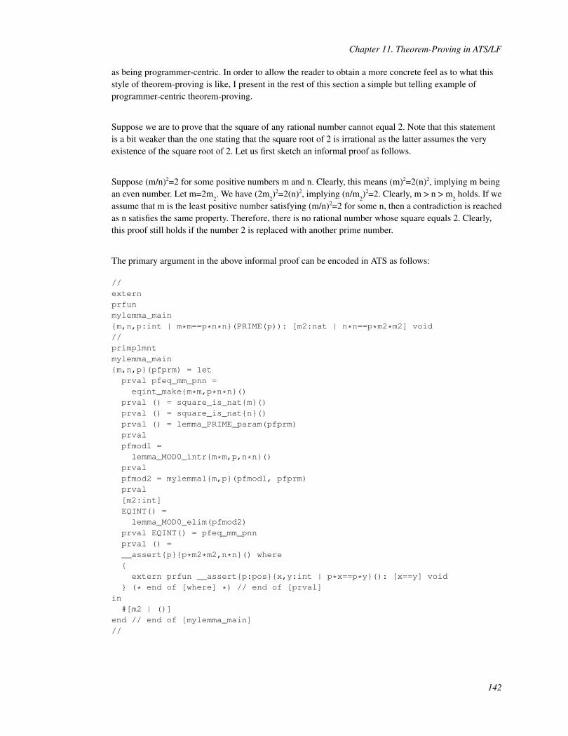
Chapter 11. Theorem-Proving in ATS/LF
as being programmer-centric. In order to allow the reader to obtain a more concrete feel as to what thisstyle of theorem-proving is like, I present in the rest of this section a simple but telling example ofprogrammer-centric theorem-proving.
Suppose we are to prove that the square of any rational number cannot equal 2. Note that this statementis a bit weaker than the one stating that the square root of 2 is irrational as the latter assumes the veryexistence of the square root of 2. Let us first sketch an informal proof as follows.
Suppose (m/n)2=2 for some positive numbers m and n. Clearly, this means (m)2=2(n)2, implying m beingan even number. Let m=2m
2. We have (2m
2)2=2(n)2, implying (n/m
2)2=2. Clearly, m > n > m
2holds. If we
assume that m is the least positive number satisfying (m/n)2=2 for some n, then a contradiction is reachedas n satisfies the same property. Therefore, there is no rational number whose square equals 2. Clearly,this proof still holds if the number 2 is replaced with another prime number.
The primary argument in the above informal proof can be encoded in ATS as follows:
//externprfunmylemma_main{m,n,p:int | m*m==p*n*n}(PRIME(p)): [m2:nat | n*n==p*m2*m2] void//primplmntmylemma_main{m,n,p}(pfprm) = letprval pfeq_mm_pnn =eqint_make{m*m,p*n*n}()
prval () = square_is_nat{m}()prval () = square_is_nat{n}()prval () = lemma_PRIME_param(pfprm)prvalpfmod1 =lemma_MOD0_intr{m*m,p,n*n}()
prvalpfmod2 = mylemma1{m,p}(pfmod1, pfprm)prval[m2:int]EQINT() =lemma_MOD0_elim(pfmod2)
prval EQINT() = pfeq_mm_pnnprval () =__assert{p}{p*m2*m2,n*n}() where{extern prfun __assert{p:pos}{x,y:int | p*x==p*y}(): [x==y] void
} (* end of [where] *) // end of [prval]in
#[m2 | ()]end // end of [mylemma_main]//
142

Chapter 11. Theorem-Proving in ATS/LF
The interface for mylemma_main states that (m)2=p(n)2 implies (n)2=p(m2)2 for some natural number m
2.
Given two integers m and p, MOD0(m,p) means that m equals the product of p and q for some naturalnumber q. This meaning is encoded into the following two proof functions:
//prfunlemma_MOD0_intr{m,p,q:nat | m==p*q}(): MOD0(m, p)//prfunlemma_MOD0_elim{m,p:int}(MOD0(m, p)): [q:nat] EQINT(m, p*q)//
where EQINT is a dataprop declared as follows:
dataprop EQINT(int, int) = {x:int} EQINT(x, x)
Given two integers x and y, EQINT(x, y) simply means that x equals y. Also, the function eqint_make isassgined the interface below:
prfun eqint_make{x,y:int | x == y}((*void*)): EQINT (x, y)
Given an integer p, PRIME(p) means that p is a prime number. The following two proof functions arecalled in the above implementation of mylemma_main:
//prfun lemma_PRIME_param{p:int}(PRIME(p)): [p >= 2] void//prfun mylemma1{n,p:int}(MOD0(n*n, p), PRIME(p)): MOD0(n, p)//
The proof function mylemma1 encodes a proposition stating that p divides n if p divides the square of nand p is also a prime number. I give no implementation of mylemma1 as I see the encoded proposition tobe obviously true. Certainly, this is a kind of programmer-centric judgment.
One may find that the following declaration in the implementation of mylemma_main looks mysterious:
prval EQINT() = pfeq_mm_pnn
Note that pfeq_mm_pnn is of the prop EQINT(m*m, p*(n*n)). Also, m equaling p*m2
for some naturalnumber m
2is available when the above declaration is typechecked. This means that the equality between
(p*m2)2 and p*(n)2 is added into the current store of (static) assumptions after the above declaration is
typechecked.
Please find on-line (https://github.com/ats-lang/ats-lang.github.io/blob/master/DOCUMENT/INT2PROGINATS/CODE/CHAP_THMPRVING/sqrt2_irrat.dats)the entirety of an encoded proof showing that there exists no rational number whose square equals 2.
143

Chapter 12. Programming withTheorem-Proving
Programming with Theorem-Proving (PwTP) is a rich and broad programming paradigm that allowscohesive construction of programs and proofs in a syntactically intwined manner. The support for PwTPin ATS is a signatory feature of ATS, and the novelty of ATS largely stems from it. For people who arefamiliar with the so-called Curry-Howard isomorphism, I emphasize that PwTP as is supported in ATSmakes little, if any, essential use of this isomorphism (between proofs and programs): The dynamics ofATS in which programs are written is certainly not pure and the proofs encoded in ATS/LF are notrequired to be constructive, either. However, that proof construction in ATS can be done in a style of(functional) programming is fundamentally important in terms of syntax design for ATS, for the need tocombine programs with proofs would otherwise be greatly more challenging.
In this chapter, I will present some simple but convincing examples to illustrate the power and flexibilityof PwTP as is supported in ATS. However, the real showcase for PwTP will not arrive until after theintroduction of linear types in ATS, when linear proofs can be combined with programs to track andsafely manipulate resources such as memory and objects (e.g, file handles). In particular, PwTP is toform the cornersone of the support for imperative programming in ATS.
Please find on-line (https://github.com/ats-lang/ats-lang.github.io/blob/master/DOCUMENT/INT2PROGINATS/CODE/CHAP_PRGTHMPRV/) the codeemployed for illustration in this chapter plus some additional code for testing.
12.1. Circumventing Nonlinear Constraints
The constraint-solver of ATS is of rather diminished power. In particular, constraints containingnonlinear integer terms (e.g., those involving the use of multiplication (of variables)) are immediatelyrejected. This weakness must be properly addressed for otherwise it would become a crippling limitationon practicality of the type system of ATS. I now use a simple example to demonstrate howtheorem-proving can be employed to circumvent the need for handling nonlinear constraints directly.
A function template list_concat is implemented as follows:
//// [list_concat] does typecheck in ATS2// [list_concat] does not typecheck in ATS1//fun{a:t@ype} list_concat{m,n:nat}(xss: list (list (a, n), m)
) : list (a, m * n) =
144
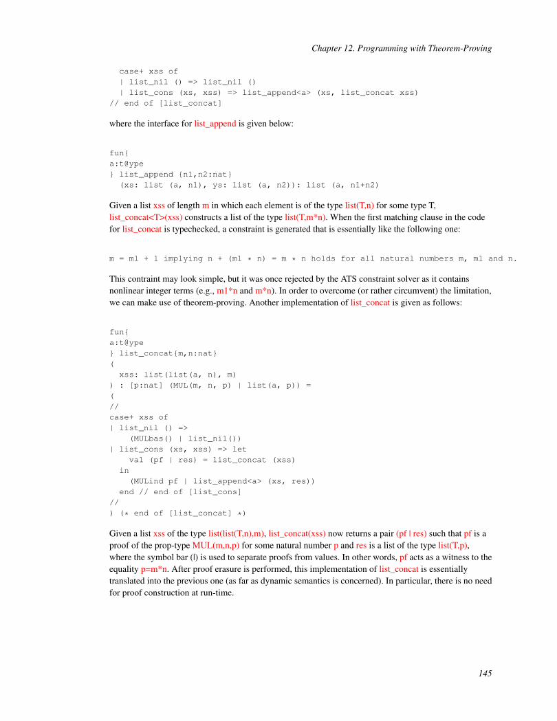
Chapter 12. Programming with Theorem-Proving
case+ xss of| list_nil () => list_nil ()| list_cons (xs, xss) => list_append<a> (xs, list_concat xss)
// end of [list_concat]
where the interface for list_append is given below:
fun{a:t@ype} list_append {n1,n2:nat}(xs: list (a, n1), ys: list (a, n2)): list (a, n1+n2)
Given a list xss of length m in which each element is of the type list(T,n) for some type T,list_concat<T>(xss) constructs a list of the type list(T,m*n). When the first matching clause in the codefor list_concat is typechecked, a constraint is generated that is essentially like the following one:
m = m1 + 1 implying n + (m1 * n) = m * n holds for all natural numbers m, m1 and n.
This contraint may look simple, but it was once rejected by the ATS constraint solver as it containsnonlinear integer terms (e.g., m1*n and m*n). In order to overcome (or rather circumvent) the limitation,we can make use of theorem-proving. Another implementation of list_concat is given as follows:
fun{a:t@ype} list_concat{m,n:nat}(xss: list(list(a, n), m)
) : [p:nat] (MUL(m, n, p) | list(a, p)) =(//case+ xss of| list_nil () =>
(MULbas() | list_nil())| list_cons (xs, xss) => let
val (pf | res) = list_concat (xss)in(MULind pf | list_append<a> (xs, res))
end // end of [list_cons]//) (* end of [list_concat] *)
Given a list xss of the type list(list(T,n),m), list_concat(xss) now returns a pair (pf | res) such that pf is aproof of the prop-type MUL(m,n,p) for some natural number p and res is a list of the type list(T,p),where the symbol bar (|) is used to separate proofs from values. In other words, pf acts as a witness to theequality p=m*n. After proof erasure is performed, this implementation of list_concat is essentiallytranslated into the previous one (as far as dynamic semantics is concerned). In particular, there is no needfor proof construction at run-time.
145

Chapter 12. Programming with Theorem-Proving
12.2. Example: Safe Matrix Subscripting
Internally, a matrix of the dimension m by n is represented as an array of the size m*n. For matrixsubscripting, we need to implement a function template of the following interface:
fun{a:t@ype} matrix_get{m,n:int}{i,j:nat | i < m; j < n}(A: arrayref (a, m*n), col: int n, i: int i, j: int j): (a)
// end of [matrix_get]
Assume that the matrix is represented in the row-major style. Then the element indexed by i and j in thematrix is the element indexed by i*n + j in the array that represents the matrix, where i and j are naturalnumbers less than m and n, respectively. However, the following implementation fails to passtypechecking:
implement{a}(*tmp*)matrix_get (A, n, i, j) = A[i*n+j] // it fails to typecheck!!!
The simple reason for this failure is due to the ATS constraint solver not being able to automaticallyverify that i*n+j is a natural number strictly less than m*n. An implementation of matrix_get thattypechecks can be given as follows:
implement{a}(*tmp*)matrix_get{m,n}{i,j}(A, n, i, j) = let
//val (pf | _in_) = imul2 (i, n)
//prval ((*void*)) = mul_elim(pf)prval ((*void*)) = mul_nat_nat_nat(pf)prval ((*void*)) = mul_gte_gte_gte{m-1-i,n}()
//inA[_in_+j]
end // end of [matrix_get]
where the functions called in the body of matrix_get are assigned the following interfaces:
//funimul2{i,j:int}(int i, int j):<> [ij:int] (MUL(i, j, ij) | int ij)
//prfun
146

Chapter 12. Programming with Theorem-Proving
mul_elim{i,j:int}{ij:int} (pf: MUL(i, j, ij)): [i*j==ij] void
//prfunmul_nat_nat_nat{i,j:nat}{ij:int} (pf: MUL(i, j, ij)): [ij >= 0] void
//prfunmul_gte_gte_gte{m,n:int | m >= 0; n >= 0} ((*void*)): [m*n >= 0] void
//
Assume that m and n are natural numbers and i and j are natural numbers less than m and n, respectively.The proof code employed in the implementation of matrix_get to show i*n+j < m*n proves (m-1-i)*n >=0, which clearly implies m*n >= i*n+n > i*n+j.
Note that there are a variety of proof functions declared in arith_prf.sats (https://github.com/ats-lang/ats-lang.github.io/blob/master/DOCUMENT/ATS-Postiats/prelude/SATS/arith_prf.sats) for helping provetheorems involving arithmetic operations. For examples of proof construction in ATS, please find theimplementation of some of these proof functions in arith_prf.dats (https://github.com/ats-lang/ats-lang.github.io/blob/master/DOCUMENT/ATS-Postiats/prelude/DATS/arith_prf.dats).
The entirety of the above presented code is available on-line (https://github.com/ats-lang/ats-lang.github.io/blob/master/DOCUMENT/INT2PROGINATS/CODE/CHAP_PRGTHMPRV/matget.dats).
12.3. Specifying with Enhanced Precision
The integer addition function can be assigned the following (dependent) type in ATS to indicate that itreturns the sum of its two integer arguments:
{i,j:int} (int(i), int(j)) -> int(i+j)
This type gives a full specification of integer addition as the only (terminating) function that can be giventhe type is the integer addition function. However, the factorial function, which yields the product of thefirst n positive integers when applied to a natural number n, cannot be given the following type:
{n:int | n >= 0} int(n) -> int(fact(n))
as fact, which refers to the factorial function, does not exist in the statics of ATS. Evidently, a highlyinteresting and relevant question is whether a type can be formed in ATS that fully captures thefunctional relation specified by fact? The answer is affirmative. We can not only construct such a type butalso assign it to a (terminating) function implemented in ATS.
Let us recall that the factorial function can be defined by the following two equations:
fact(0) = 1
147

Chapter 12. Programming with Theorem-Proving
fact(n) = n * fact(n-1) (for all n > 0)
Naturally, these equations can be encoded by the constructors associated with the dataprop FACTdeclared as follows:
datapropFACT(int, int) =| FACTbas(0, 1)| {n:nat}{r1,r:int}FACTind(n, r) of (FACT(n-1, r1), MUL(n, r1, r))
// end of [FACT]
Note that for any given natural number n and integer r, FACT(n, r) can be assigned to a proof if and onlyif fact(n) equals r. Therefore, the following type:
{n:nat} int(n) -> [r:int] (FACT(n, r) | int(r))
can only be assigned to a function that, if applied to a natural number n, returns a proof and an integersuch that the proof attests to the integer being equal to fact(n). For instance, the following definedfunction ifact is assigned this type:
//funifact{n:nat} .<n>.(n: int(n)
) :<> [r:int] (FACT(n, r) | int r) =(//ifn = 0then (FACTbas() | 1)else letval (pf1 | r1) = ifact (n-1) // pf1: FACT(n-1, r1)val (pfmul | r) = imul2 (n, r1) // pfmul: FACT(n, r1, r)
in(FACTind(pf1, pfmul) | r)
end // end of [else]//) (* end of [ifact] *)//
After proof erasure, ifact precisely implements the factorial function.
Please find the entirety of the above presented code plus some testing code on-line(https://github.com/ats-lang/ats-lang.github.io/blob/master/DOCUMENT/INT2PROGINATS/CODE/CHAP_PRGTHMPRV/ifact.dats).
148

Chapter 12. Programming with Theorem-Proving
12.4. Example: Another Verified Factorial
The function ifact presented in the section on specifying with enhanced precision is a verifiedimplementation of the factorial function as its type guarantees that ifact implements the specification offactorial encoded by the dataprop FACT. Clearly, the implementation of ifact closely follows thedeclaration of FACT. If we think of the latter as a logic program, then the former is essentially afunctional version extracted from the logic program. However, the implementation of a specification inpractice can often digress far from the specification algorithmically. For instance, we may want to have averified implementation of factorial that is also tail-recursive. This can be done as follows:
funifact2{n:nat} .<>.(n: int (n)
) :<> [r:int] (FACT(n, r) | int r) = letfun loop{i:nat|i <= n}{r:int} .<n-i>.
(pf: FACT(i, r)
| n: int n, i: int i, r: int r) :<> [r:int] (FACT(n, r) | int r) =if n - i > 0 then letval (pfmul | r1) = imul2 (i+1, r) in loop (FACTind(pf, pfmul) | n, i+1, r1)
end else (pf | r) // end of [if]// end of [loop]
inloop (FACTbas() | n, 0, 1)
end // end of [ifact2]
The function ifact2 is assigned a type indicating that ifact2 is a verified implementation of factorial, andit is defined as a call to the inner function loop that is clearly tail-recursive. If we erase types and proofs,the function ifact2 is essentially defined as follows:
fun ifact2 (n) = letfun loop (n, i, r) =if n - i > 0 then letval r1 = (i+1) * r in loop (n, i+1, r1)
end else r // end of [if]// end of [loop]
inloop (n, 0, 1)
end // end of [ifact2]
When the inner function loop is called on three arguments n, i and r, the precondition for this call is that iis natural number less than or equal to n and r equals fact(i), that is, the value of the factorial function oni. This precondition is captured by the type assigned to loop and thus enforced at each call site of loop inthe implementation of ifact2.
149

Chapter 12. Programming with Theorem-Proving
Please find on-line (https://github.com/ats-lang/ats-lang.github.io/blob/master/DOCUMENT/INT2PROGINATS/CODE/CHAP_PRGTHMPRV/ifact23.dats)the entirety of the above presented code plus some testing code.
12.5. Example: Verified Fast Exponentiation
Given an integer x, pow(x, n), the nth power of x, can be defined inductively as follows:
pow (x, 0) = 1pow (x, n) = x * pow (x, n-1) (for all n > 0)
A direct implementation of this definition is given as follows:
fun ipow {n:nat} .<n>.(x: int, n: int n): int = if n > 0 then x * ipow (x, n-1) else 1
// end of [ipow]
which is of time-complexity O(n) (assuming multiplication is O(1)). A more efficient implmentation canbe given as follows:
funifastpow{n:nat} .<n>.(x: int, n: int n
) : int =if n > 0 then letval n2 = half(n)val i2 = n-(2*n2)
inif i2 > 0 then ifastpow (x*x, n2) else x * ifastpow (x*x, n2)
end else 1 // end of [if]// end of [ifastpow]
which makes use of the property that pow(x, n) equals pow(x*x, n/2) if n is even or x * pow(x*x, n/2) ifn is odd. This is referred to as fast exponentiation. Note that ifastpow is of time-complexity O(log(n)).
Clearly, what is done above is not restricted to exponentiation on integers. As long as the underlyingmultiplication is associative, fast exponentiation can be employed to compute powers of any givenelement. In particular, powers of square matrices can be computed in this way. I now present as follows averified generic implementation of fast exponentiation.
Handling generic data properly in a verified implementation often requires some finesse with the typesystem of ATS. Let us first introduce an abstract type constructor ELT as follows:
sortdef elt = int // [elt] is just an alias for [int]
150

Chapter 12. Programming with Theorem-Proving
abst@ype ELT(a:t@ype, x:elt) = a // [x] is an imaginary stamp
This is often referred to as stamping. For each type T and stamp x, ELT(T, x) is just T as far as datarepresentation is concerned. The stamps are imaginary and they are solely used for the purpose ofspecification. Let us next introduce an abstract prop-type MUL and a function template mul_elt_elt:
//absprop MUL(elt, elt, elt) // abstract mul relation//fun{a:t@ype}mul_elt_elt{x,y:elt}(x: ELT(a, x), y: ELT(a, y)): [xy:elt] (MUL(x, y, xy) | ELT(a, xy))
// end of [mul_elt_elt]//
Please do not confuse MUL with the one of the same name that is declared in arith_prf.sats(https://github.com/ats-lang/ats-lang.github.io/blob/master/DOCUMENT/ATS-Postiats/prelude/SATS/arith_prf.sats). To state that the encoded multiplication is associative, we canintroduce the following proof function:
praximul_assoc{x,y,z:elt}{xy,yz:elt}{xy_z,x_yz:elt}(MUL(x, y, xy), MUL(xy, z, xy_z), MUL(y, z, yz), MUL(x, yz, x_yz)
) : [xy_z==x_yz] void // end of [mul_assoc]
The keyword praxi indicates that mul_assoc is treated as a form of axiom, which is not expected to beimplemented.
The abstract power function can be readily specified in terms of the abstract prop-type MUL:
datapropPOW (elt(*base*), int(*exp*), elt(*res*)
) = // res = base^exp| {x:elt}POWbas(x, 0, 1(*unit*))
| {x:elt}{n:nat}{p,p1:elt}POWind(x, n+1, p1) of (POW(x, n, p), MUL(x, p, p1))
// end of [POW]
As can be expected, generic fast exponentiation is given the following interface:
fun{a:t@ype}fastpow_elt_int{x:elt}{n:nat}(x: ELT(a, x), n: int n): [p:elt] (POW(x, n, p) | ELT(a, p))
// end of [fastpow_elt_int]
151

Chapter 12. Programming with Theorem-Proving
With the preparation done above, a straightforward implementation of fastpow_elt_int can now bepresented as follows:
implement{a}(*tmp*)fastpow_elt_int(x, n) = let
//(*lemma: (x*x)^n = x^(2n)
*)externprfunlemma{x:elt}{xx:elt}{n:nat}{y:elt}(pfxx: MUL(x, x, xx), pfpow: POW(xx, n, y)): POW(x, 2*n, y)
//overload * with mul_elt_elt // [*] loaded with mul_elt_elt//in//ifn = 0then letval res = mulunit<a> () in (POWbas () | res) // res = 1
end // end of [then]else letval n2 = half nval (pfxx | xx) = x * xval (pfpow2 | res) = fastpow_elt_int<a> (xx, n2) // xx^n2 = resprval pfpow = lemma (pfxx, pfpow2) // pfpow: x^(2*n2) = res
inif n=2*n2then (pfpow | res)else letval (pfmul | xres) = x * res in (POWind(pfpow, pfmul) | xres)
end // end of [else]end // end of [else]//end // end of [fastpow_elt_int]
Note that this implementation of fastpow_elt_int is not tail-recursive. The function template mulunit,which is called to produce a unit for the underlying multiplication, is assigned the following interface:
fun{a:t@ype} mulunit (): ELT(a, 1(*stamp*))
The proof function lemma simply establishes that pow(x, 2*n)= pow(x*x, n) for each natural number n. Ihave made an implementation of lemma available on-line but I suggest that the interested reader give it a
152
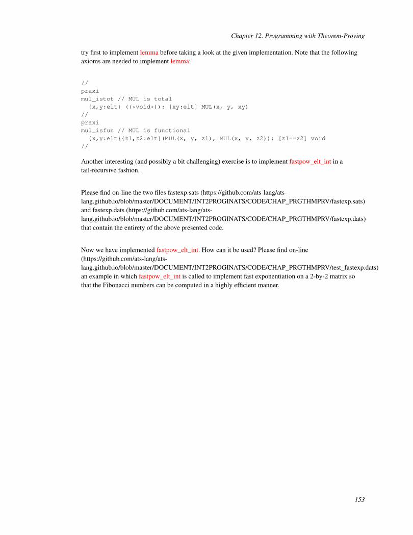
Chapter 12. Programming with Theorem-Proving
try first to implement lemma before taking a look at the given implementation. Note that the followingaxioms are needed to implement lemma:
//praximul_istot // MUL is total{x,y:elt} ((*void*)): [xy:elt] MUL(x, y, xy)
//praximul_isfun // MUL is functional{x,y:elt}{z1,z2:elt}(MUL(x, y, z1), MUL(x, y, z2)): [z1==z2] void
//
Another interesting (and possibly a bit challenging) exercise is to implement fastpow_elt_int in atail-recursive fashion.
Please find on-line the two files fastexp.sats (https://github.com/ats-lang/ats-lang.github.io/blob/master/DOCUMENT/INT2PROGINATS/CODE/CHAP_PRGTHMPRV/fastexp.sats)and fastexp.dats (https://github.com/ats-lang/ats-lang.github.io/blob/master/DOCUMENT/INT2PROGINATS/CODE/CHAP_PRGTHMPRV/fastexp.dats)that contain the entirety of the above presented code.
Now we have implemented fastpow_elt_int. How can it be used? Please find on-line(https://github.com/ats-lang/ats-lang.github.io/blob/master/DOCUMENT/INT2PROGINATS/CODE/CHAP_PRGTHMPRV/test_fastexp.dats)an example in which fastpow_elt_int is called to implement fast exponentiation on a 2-by-2 matrix sothat the Fibonacci numbers can be computed in a highly efficient manner.
153

IV. Programming with Views andViewtypes

Chapter 13. Introduction to Views andViewtypes
Probably the single greatest motivation behind the development of ATS is the desire to make ATS aprogramming language that can be employed effectively to construct safe and reliable programs runningin the kernels of operating systems. Instead of following seemingly natural approaches that often focuson carving out a "safe" subset of C and/or put wrappers around "unsafe" programming features in C,ATS relies on the paradigm of programming with theorem-proving to prevent resources such as memoryfrom being misused or mismanaged, advocating an approach to safety that is both general and flexible.For example, a well-typed program constructed in ATS cannot cause buffer overrun at run-time eventhough pointer arithmetic is fully supported in ATS. More specifically, if a pointer is to be dereferenced,ATS requires that a proof be given attesting to the safety of the dereferencing operation. Proofs of thiskind are constructed to demonstrate the validity of linear propositions, which are referred to as views inATS, for classifying resources as well as capabilities.
Please find on-line (https://github.com/ats-lang/ats-lang.github.io/blob/master/DOCUMENT/INT2PROGINATS/CODE/CHAP_VVTINTRO/) the codepresented for illustration in this chapter.
13.1. Views for Memory Access through Pointers
A view is a linear version of prop, where the word linear comes from linear logic, a resource-aware logicinvented by Jean-Yves Girard. There is a built-in sort view for static terms representing views. Given atype T and a memory location L, a view of the form T@L can be formed to indicate a value of the type Tbeing stored in the memory at the location L, where @ is a special infix operator. Views of this form areextremely common in practice, and they are often referred to as at-views. As an example, the followingfunction templates ptr_get0 and ptr_set0, which reads and writes through a given pointer, are assignedtypes containing at-views:
//fun{a:t@ype}ptr_get0 {l:addr} (pf: a @ l | p: ptr l): (a @ l | a)//fun{a:t@ype}ptr_set0 {l:addr} (pf: a? @ l | p: ptr l, x: a): (a @ l | void)//
Note that ptr is a type constructor that forms a type ptr(L) when applied to a static term L of the sortaddr, and the only value of the type ptr(L) is the pointer that points to the location denoted by L.
155

Chapter 13. Introduction to Views and Viewtypes
Given a type T, the function ptr_get0<T> is assigned the following type:
{l:addr} (T @ l | ptr (l)) -> (T @ l | T)
which indicates that the function ptr_get0<T> returns a proof of the view T@L and a value of the type Twhen applied to a proof of the view T@L and a pointer of the type ptr(L) for some L. Intuitivelyspeaking, a proof of the view T@L, which is a form of resource as T@L is linear, is consumed when it ispassed to ptr_get0<T>, and another proof of the same view T@L is generated when ptr_get0<T> returns.Notice that a proof of the view T@L must be returned for otherwise subsequent accesses to the memorylocation L would have been precluded.
Similarly, the function ptr_set0<T> is assigned the following type:
{l:addr} (T? @ l | ptr (l), T) -> (T @ l | void)
Note that T? is a type for values of size sizeof(T) that are assumed to be uninitialized. The functionptr_set0<T> returns a proof of the view T@L when applied to a proof of the view T?@L, a pointer of thetype ptr(L) and a value of the type T. The use of the view T?@L indicates that the memory location at Lis assumed to be uninitialized when ptr_set0<T> is called.
As an example, a function template swap0 is implemented as follows for swapping memory contents attwo given locations:
fn{a:t@ype}swap0{l1,l2:addr}(pf1: a @ l1, pf2: a @ l2
| p1: ptr (l1), p2: ptr (l2)) : (a @ l1, a @ l2 | void) = letval (pf1 | x1) = ptr_get0<a> (pf1 | p1)val (pf2 | x2) = ptr_get0<a> (pf2 | p2)val (pf1 | ()) = ptr_set0<a> (pf1 | p1, x2)val (pf2 | ()) = ptr_set0<a> (pf2 | p2, x1)
in(pf1, pf2 | ())
end // end of [swap0]
Compared to a corresponding implementation in C, the verbosity of this one in ATS is evident. Inparticular, the need for threading linear proofs through calls to functions that make use of resources canoften result in a lot of administrative code to be written. I now present some special syntax tosignificantly alleviate the need for such administrative code.
The function templates ptr_get1 and ptr_set1 are given the following interfaces:
//fun{a:t@ype}
156

Chapter 13. Introduction to Views and Viewtypes
ptr_get1 {l:addr} (pf: !a @ l >> a @ l | p: ptr l): a//fun{a:t@ype}ptr_set1 {l:addr} (pf: !a? @ l >> a @ l | p: ptr l, x: a): void//
Clearly, for each type T, the function ptr_get1<T> is assigned the following type:
{l:addr} (!T @ l >> T @ l | ptr(l)) -> T
Given a linear proof pf of the view T@L for some L and a pointer p of the type ptr(L), the function callptr_get1<T>(pf, p) is expected to return a value of the type T. However, the proof pf is not consumed.Instead, it is still a proof of the view T@L after the function call returns. Similarly, the functionptr_set1<T> is assigned the following type:
{l:addr} (!T? @ l >> T @ l | ptr(l), T) -> void
Given a linear proof pf of the view T?@L for some L, a pointer p of the type ptr(L) and a value v of thetype T, the function call ptr_set1<T>(pf, p, v) is expected to return the void value while changing theview of pf from T?@L to T@L. In general, assume that f is given a type of the following form for someviews V1 and V2:
(...,!V1 >> V2, ...) -> ...
Then a function call f(..., pf, ...) on some proof variable pf of the view V1 is to change the view of pf intoV2 upon its return. In the case where V1 and V2 are the same, !V1 >> V2 can simply be written as !V1.As an example, a function template swap1 for swapping the contents at two given memory locations isimplemented as follows:
fn{a:t@ype}swap1{l1,l2:addr}(pf1: !a@l1, pf2: !a@l2 | p1: ptr l1, p2: ptr l2
) : void = letval x = ptr_get1<a> (pf1 | p1)val () = ptr_set1<a> (pf1 | p1, ptr_get1<a> (pf2 | p2))val () = ptr_set1<a> (pf2 | p2, x)
in// nothing
end // end of [swap1]
Clearly, this implementation is considerably cleaner when compared to the above implementation ofswap0.
A further simplied implementation of swap1 is given as follows:
fn{a:t@ype}swap1{l1,l2:addr}
157

Chapter 13. Introduction to Views and Viewtypes
(pf1: !a@l1, pf2: !a@l2
| p1: ptr (l1), p2: ptr (l2)) : void = letval tmp = !p1 in !p1 := !p2; !p2 := tmp
end // end of [swap1]
Given a pointer p of the type ptr(L) for some L, !p yields the value stored at the memory location L. Thetypechecker first searches for a proof of the view T@L for some T among all the currently availableproofs when typechecking !p; if such a proof pf is found, then !p is essentially elaborated intoptr_get1(pf | p) and then typechecked. As !p is a left-value (which is to be explained later in detail), it canalso be used to form an assignment like !p := v for some value v. The typechecker elaborates !p := v intoptr_set1(pf | p, v) for the sake of typechecking if a proof of the at-view T@L can be found for some typeT among all the currently available proofs. Note that this implementation of swap1 makes no use ofadministrative code for handling linear proofs explicitly.
13.2. Viewtypes as a Combination of Views and Types
A linear type in ATS is given the name viewtype, which is chosen to indicate that a linear type consists oftwo parts: one part for views and the other for types. For instance, given a view V and a type T, then thetuple (V | T) is a viewtype, where the bar symbol (|) is a separator (just like a comma) to separate viewsfrom types. What seems a bit surprising is the opposite: For each viewtype VT, we may assume theexistence of a view V and a type T such that VT is equivalent to (V | T). Formally, this T can be referredas VT?! in ATS. This somewhat unexpected interpretation of linear types is a striking novelty of ATS,which stresses that the linearity of a viewtype comes entirely from the view part residing within it.
The built-in sorts viewtype and viewt@ype are for static terms representing viewtypes whose type partsare of the sorts type and t@ype, respectively. In other words, the former is assigned to viewtypes forlinear values of the size equal to that of a pointer and the latter to viewtypes for linear values ofunspecified size. For example, tptr is defined as follows that takes a type and an address to form aviewtype (of the sort viewtype):
vtypedef tptr (a:t@ype, l:addr) = (a @ l | ptr l)
Given a type T and an address L, the viewtype tptr(T, L) is for a pointer to L paired with a linear proofstating that a value of the type T is stored at L. If we think of a counter as a pointer paired with a proofstating that the pointer points to an integer (representing the count), then the following defined functiongetinc returns the current count of a given counter after increasing it by 1:
fn getinc{l:addr}{n:nat}
(cnt: !tptr (int(n), l) >> tptr (int(n+1), l)
) : int(n) = n where {val n = ptr_get1<int(n)> (cnt.0 | cnt.1)val () = ptr_set1<int(n+1)> (cnt.0 | cnt.1, n+1)
} (* end of [getinc] *)
158
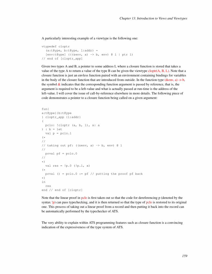
Chapter 13. Introduction to Views and Viewtypes
A particularly interesting example of a viewtype is the following one:
vtypedef cloptr(a:t@ype, b:t@ype, l:addr) =[env:t@ype] (((&env, a) -> b, env) @ l | ptr l)
// end of [cloptr_app]
Given two types A and B, a pointer to some address L where a closure function is stored that takes avalue of the type A to return a value of the type B can be given the viewtype cloptr(A, B, L). Note that aclosure function is just an envless function paired with an environment containing bindings for variablesin the body of the closure function that are introduced from outside. In the function type (&env, a) -> b,the symbol & indicates that the corresponding function argument is passed by reference, that is, theargument is required to be a left-value and what is actually passed at run-time is the address of theleft-value. I will cover the issue of call-by-reference elsewhere in more details. The following piece ofcode demonstrates a pointer to a closure function being called on a given argument:
fun{a:t@ype}{b:t@ype} cloptr_app {l:addr}(pclo: !cloptr (a, b, l), x: a
) : b = letval p = pclo.1
(*//// taking out pf: ((&env, a) -> b, env) @ l//prval pf = pclo.0
//
*)val res = !p.0 (!p.1, x)
(*prval () = pclo.0 := pf // putting the proof pf back
*)inres
end // end of [cloptr]
Note that the linear proof in pclo is first taken out so that the code for dereferencing p (denoted by thesyntax !p) can pass typechecking, and it is then returned so that the type of pclo is restored to its originalone. This process of taking out a linear proof from a record and then putting it back into the record canbe automatically performed by the typechecker of ATS.
The very ability to explain within ATS programming features such as closure function is a convincingindication of the expressiveness of the type system of ATS.
159

Chapter 13. Introduction to Views and Viewtypes
13.3. Left-Values and Call-by-Reference
In its simplest form, a left-value is just a pointer paired with a linear proof attesting to a value (of sometype) being stored at the location to which the pointer points. The name left-value stems from such avalue being allowed to appear on the left-hand side of an assignment statement (in languages like C).Often, a left-value is intuitively explained as a value with an address attached to it. Note that whateverrepresentation chosen for a left-value must make it possible to identify both the pointer and the linearproof (of some at-view) that are associated with the left-value.
In ATS, the simplest expression representing a left-value is !p, where ! is a special symbol and p a valueof the type ptr(L) for some address L. When this expression is typechecked, a proof of T@L for sometype T is required to be found among the currently available proofs. I will introduce additional forms ofleft values gradually.
The default strategy for passing a function argument in ATS is call-by-value. However, it is also allowedin ATS to specify that call-by-reference is chosen for passing a particular function argument. Bycall-by-reference, it is meant that the argument to be passed must be a left-value and what is actuallypassed is the address of the left-value (instead of the value stored at the address). For example, thefollowing defined function swap2 makes essential use of call-by-reference:
fn{a:t@ype} swap2 (x1: &a, x2: &a
) : void = letval tmp = x1 in x1 := x2; x2 := tmp
end // end of [swap2]
Note that the special symbol & in front of the type of a function argument indicates that the argumentneeds to be passed according to the call-by-reference strategy. The following code implements swap1based on swap2:
fn{a:t@ype} swap1{l1,l2:addr}(pf1: !a @ l1, pf2: !a @ l2 | p1: ptr l1, p2: ptr l2
) : void = swap2 (!p1, !p2)
When the call swap2(!p1, !p2) is evaluated at run-time, the parameters actually being passed are the twopointers p1 and p2 (rather than the values stored at the locations to which these two pointers point).
Given a type T and an integer N, the syntax @[T][N] stands for a flat array consisting N elements of thetype T. Please note that a value of the type @[T][N] is of the size N*sizeof(T). If a function has aparameter representing an array, then this parameter is most liklely call-by-reference. For instance, thefollowing code implements a function that takes two arrays of doubles to compute their dot product (alsoknowns as inner product):
160

Chapter 13. Introduction to Views and Viewtypes
fun dotprod(A: &(@[double][3])
, B: &(@[double][3])) : double =(A[0] * B[0] + A[1] * B[1] + A[2] * B[2]
)
Note that both array arguments of dotprod are call-by-reference.
13.4. Stack-Allocated Variables
Given a type T and an address L, how can a proof of the view T@L be obtained in the first place? Thereare actually a variety of methods for obtaining such proofs in practice, and I present one as follows that isbased on stack-allocation of local variables.
In the body of the following function foo, some stack-allocated local variables are declared:
fn foo (): void = letvar x0: int // view@(x0): int? @ x0val () = x0 := 0 // view@(x0): int(0) @ x0var x1: int = 1 // view@(x1): int(1) @ x1
//// [with] is a keyword in ATS//var y: int with pfy // pfy is an alias of view@(y): int? @ yval () = y := 2 // pfy = view@(y): int(2) @ yvar z: int with pfz = 3 // pfz is an alias of view@(z): int(3) @ z
in// nothing
end // end of [foo]
The keyword var is for declaring a local variable. When a variable is declared, either its type or its initialvalue needs to be given. If a variable is declared without a type, then the type of its initial value isassumed to be its type. Assume that a variable x is declared of type T. Then the pointer to the location ofthe variable is denoted by addr@(x), where addr@ is a keyword, and its associated linear proof (of someat-view) can be referred to as view@(x), where view@ is a keyword. A variable is another form ofleft-value in ATS. In the body of foo, x0 is declared to be a variable of the type int and then it isinitialized with the integer 0; x1 is declared to be a variable of the type int that is given the initial value 1;y is declared to be a variable of the type int while pfy is introduced as an alias for view@(y), and then yis initialized with the integer 2; z is declared to be a variable of the type int that is given the initial value 3while pfz is introduced as an alias for view@(z).
The following code gives an implementation of the factorial function:
fn fact{n:nat}
161

Chapter 13. Introduction to Views and Viewtypes
(n: int (n)): int = letfun loop{n:nat}{l:addr} .<n>.(pf: !int @ l | n: int n, res: ptr l): void =if n > 0 then letval () = !res := n * !res in loop (pf | n-1, res)
end // end of [if]// end of [loop]var res: int with pf = 1val () = loop (pf | n, addr@res) // addr@res: the pointer to res
inres
end // end of [fact]
Note that the variable res holds the intermediate result during the execution of the loop. As res isstack-allocated, there is no garbage generated after a call to fact is evaluated. When this style ofprogramming is done in C, there is often a concern about the pointer to res being derefenced after a callto fact returns, which is commonly referred to as derefencing a dangling pointer. This concern iscompletely eliminated in ATS as it is required by the type system of ATS that a linear proof of theat-view associated with the variable res be present at the end of legal scope for res. More specifically, if xis a declared variable of the type T, then a linear proof of the view T?@L, where L is the address of x,must be available when typechecking reaches the end of the scope for x. This requirement ensures that avariable can no longer be accessed after the portion of the stack in which it is allocated is reclaimed as nolinear proof of the at-view associated with the variable is ever available from that point on.
Arrays in ATS can also be stack-allocated. For instance, the following code allocates two arrays ofdoubles in the frame of the function main0 and then passes them to dotprod to compute their dot product:
implementmain0 () ={//var A = @[double][3](1.0) // initialized with 1.0, 1.0, 1.0var B = @[double](1.0, 2.0, 3.0) // initialized with 1.0, 2.0, 3.0//val () = println! ("A * B = ", dotprod (A, B)) // A * B = 6.0//} (* end of [main0] *)
The at-view associated with the variable A is (@[double][3])@A, where A also refers to the address ofthe variable A. Similarly, the at-view associated with the variable B is (@[double][3])@B. For the sakeof completeness, I mention the syntax for uninitialized arrays as follows: Given a type T and an integerN, the syntax @[T][N]() is for an array consisting of N uninitialized values of type T.
Note that allocating large arrays in the call frame of a function may not be a good practice as doing socan greatly increase the likelihood of stack-overflow at run-time.
162

Chapter 13. Introduction to Views and Viewtypes
It is also allowed in ATS to allocate a closure in the call frame of a function. For instance, the followingcode implements a function named foo that stores a flat closure-function in a stack-allocated variablenamed bar:
fun foo(x: int, y: int
) : int = let//var bar = lam@ (): int => x * y//inbar ()
end // end of [foo]
Note that the special keyword lam@ should be used to form a flat closure-function. For the sake ofcompleteness, I present another example as follows to show that a recursive closure-function can also bestored in a stack-allocated variable:
fun foo2(x: int, y: int
) : int = let//var bar2 = fix@ f (x: int): int => if x > 0 then y + f(x-1) else 0//inbar2 (x)
end // end of [foo]
Note that the special keyword fix@ should be used to form a flat recursive closure-function.
In a setting where dynamic memory allocation is not allowed, stack-allocated closures can play a pivotalrole in supporting programming with higher-order functions.
13.5. Heap-Allocated Linear Closure-Functions
In ATS, a closure-function can be assiged a linear type, allowing it to be properly tracked within the typesystem and also explicitly freed by the programmer.
The following code implements a higher-order function list_map_cloptr which takes a linearclosure-function as its second argument:
fun{a:t@ype}{b:vt@ype} list_map_cloptr{n:int}(
163

Chapter 13. Introduction to Views and Viewtypes
xs: list (a, n), f: !(a) -<cloptr1> b) : list_vt (b, n) =(case+ xs of| list_nil () => list_vt_nil ()| list_cons (x, xs) => list_vt_cons (f (x), list_map_cloptr<a><b> (xs, f))
)
Note that the keyword -<cloptr1> indicates that the function type it forms is for a linear closure-function.If a type for a pure linear closure-function is needed, the keyword -<cloptr0> can be used. The symbol !in front of the function type means that the second (linear) argument of list_map_cloptr is call-by-valueand it is still available after list_map_cloptr returns.
Let us now see some concrete code in which a linear closure-function is created, called, and finally freed:
implementmain0 () ={//val xs =$list_vt{int}(0, 1, 2, 3, 4)//val len = list_vt_length (xs)//val f = lam (x: int): int =<cloptr1> x * len//val ys =list_map_cloptr<int><int> ($UNSAFE.list_vt2t(xs), f)//val () = cloptr_free($UNSAFE.castvwtp0{cloptr(void)}(f))//val () = println! ("xs = ", xs) // xs = 0, 1, 2, 3, 4val () = println! ("ys = ", ys) // ys = 0, 5, 10, 15, 20//val ((*freed*)) = list_vt_free (xs)val ((*freed*)) = list_vt_free (ys)//} (* end of [main0] *)
The function cloptr_free is given the following interface:
fun cloptr_free{a:t0p}(pclo: cloptr (a)):<!wrt> void
Also, the cast involved in $UNSAFE.castvwtp0{cloptr(void)}(f) is a safe cast.
The support for linear closure-functions in ATS1 is crucial in a setting where higher-order functions areneeded but run-time garbage collection (GC) is not allowed or supported. In ATS2, linearclosure-functions become much less important as programming with higher-order functions in a settingwithout GC can be more conveniently achieved through the use of templates. However, if one wants to
164

Chapter 13. Introduction to Views and Viewtypes
store closure-functions in a data structure without causing memory leaks, it is necessary to use linearclosure-functions unless GC can be relied upon to reclaim memory.
165

Chapter 14. Dataviews as Linear Dataprops
The at-views of the form T@L for types T and addresses L are building blocks for constructing otherforms of views. One mechanism for putting together such building blocks is by declaring dataviews,which is mostly identical to declaring dataprops. I now present in this chapter some commonlyencountered dataviews and their uses.
Please find on-line (https://github.com/ats-lang/ats-lang.github.io/blob/master/DOCUMENT/INT2PROGINATS/CODE/CHAP_DATAVIEW/) the codepresented for illustration in this chapter.
14.1. Optional Views
The dataview option_v is declared as follows:
dataview option_v (v:view+, bool) =| Some_v (v, true) of (v) | None_v (v, false) of ()
This declaration indicates that the dataview option_v is covariant in its first argument and there are twoproof constructors associated with it: Some_v and None_v. Given a view V, option_v(V, b) is oftencalled an optional view, where b is a boolean. Clearly, a proof of the view option_v(V, true) contains aproof of the view V while a proof the view option_v(V, false) contains nothing.
As an example, the following function interface involves a typical use of optional view:
fun{a:t@ype}ptr_alloc_opt (): [l:addr] (option_v (a? @ l, l > null) | ptr l)
Given a type T, the function ptr_alloc_opt<T> returns a pointer paired with a proof of an optional view;if the returned pointer is not null, then the proof can be turned into a proof of the view T?@L, where L isthe location to which the pointer points; otherwise, there is no at-view associated with the returnedpointer.
14.2. Disjunctive Views
The dataview VOR is declared as follows:
dataview VOR (v0:view+, v1:view+, int) =| VORleft (v0, v1, 0) of (v0) | VORright (v0, v1, 1) of (v1)
This declaration indicates that the dataview VOR is covariant in its first and second arguments and thereare two proof constructors associated with it: VORleft and VORright. Given views V
0and V
1, a proof of
166

Chapter 14. Dataviews as Linear Dataprops
VOR(V0, V
1, 0) can be turned into a proof of V
0and a proof of VOR(V
0, V
1, 1) can be turned into a proof
of V1.
Let T be some type. The following function interface states that getopt takes an unintialized pointer andreturns an integers indicating whether the pointer is initialized:
fun getopt{l:addr}(pf: T? @ l | ptr (l)): [i:int] (VOR (T? @ l, T @ l, i) | int (i))
The following code shows a typical use of getopt:
fun foo (): void = letvar x: T?val (pfor | i) = getopt (view@(x) | addr@(x))
in//if i = 0then letprval VORleft (pf0) = pfor in view@(x) := pf0 // uninitialized
end // end of [then]else letprval VORright (pf1) = pfor in view@(x) := pf1 // initialized
end // end of [else]// end of [if]//end // end of [foo]
In ATS, there is a type constructor opt that takes a type T and a boolean B to form an opt-type opt(T, B)such that opt(T, B) equals T if B is true and it equals T? if B is false. The function getopt can be given thefollowing interface that makes use of an opt-type:
fun getopt (x: &T? >> opt (T, b)): #[b:bool] bool(b)
The code that calls getopt can now be implemented as follows:
fun foo (): void = letvar x: T?val ans = getopt (x)
in//if (ans)then letprval () = opt_unsome(x) in (*initialized*)
end // end of [then]else letprval () = opt_unnone(x) in (*uninitialized*)
end // end of [else]// end of [if]
167
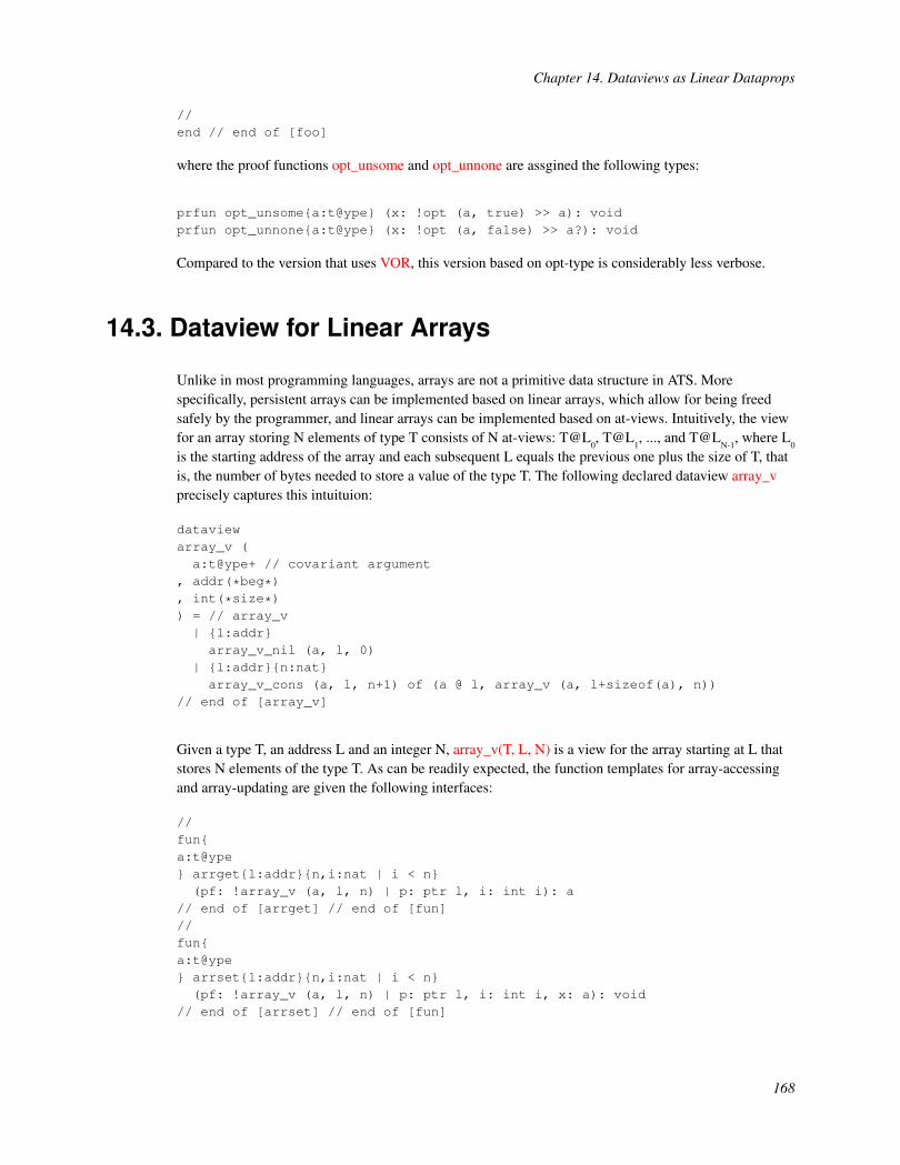
Chapter 14. Dataviews as Linear Dataprops
//end // end of [foo]
where the proof functions opt_unsome and opt_unnone are assgined the following types:
prfun opt_unsome{a:t@ype} (x: !opt (a, true) >> a): voidprfun opt_unnone{a:t@ype} (x: !opt (a, false) >> a?): void
Compared to the version that uses VOR, this version based on opt-type is considerably less verbose.
14.3. Dataview for Linear Arrays
Unlike in most programming languages, arrays are not a primitive data structure in ATS. Morespecifically, persistent arrays can be implemented based on linear arrays, which allow for being freedsafely by the programmer, and linear arrays can be implemented based on at-views. Intuitively, the viewfor an array storing N elements of type T consists of N at-views: T@L
0, T@L
1, ..., and T@L
N-1, where L
0is the starting address of the array and each subsequent L equals the previous one plus the size of T, thatis, the number of bytes needed to store a value of the type T. The following declared dataview array_vprecisely captures this intuituion:
dataviewarray_v (a:t@ype+ // covariant argument
, addr(*beg*), int(*size*)) = // array_v| {l:addr}array_v_nil (a, l, 0)
| {l:addr}{n:nat}array_v_cons (a, l, n+1) of (a @ l, array_v (a, l+sizeof(a), n))
// end of [array_v]
Given a type T, an address L and an integer N, array_v(T, L, N) is a view for the array starting at L thatstores N elements of the type T. As can be readily expected, the function templates for array-accessingand array-updating are given the following interfaces:
//fun{a:t@ype} arrget{l:addr}{n,i:nat | i < n}(pf: !array_v (a, l, n) | p: ptr l, i: int i): a
// end of [arrget] // end of [fun]//fun{a:t@ype} arrset{l:addr}{n,i:nat | i < n}(pf: !array_v (a, l, n) | p: ptr l, i: int i, x: a): void
// end of [arrset] // end of [fun]
168

Chapter 14. Dataviews as Linear Dataprops
//
Before implementing arrget and arrset, I present as follows some code that implements a functiontemplate to access the first element of a nonempty array:
fun{a:t@ype} arrgetfst{l:addr}{n:pos}(pf: !array_v (a, l, n) | p: ptr l
) : a = x where {prval array_v_cons (pf1, pf2) = pf// pf1: a @ l; pf2: array_v (a, l+sizeof(a), n-1)val x = !pprval () = pf := array_v_cons (pf1, pf2)
} // end of [arrgetfst]
Obviously, the function template arrget can be implemented based on arrgetfst:
implement{a}(*tmp*)arrget (pf | p, i) =if i > 0 then letprval array_v_cons (pf1, pf2) = pfval x = arrget (pf2 | ptr_succ<a> (p), i-1)prval () = pf := array_v_cons (pf1, pf2)
inx
end elsearrgetfst (pf | p)
// end of [if]
This is a tail-recursive implementation of time-complexity O(n). However, the very point of havingarrays is to support O(1)-time accessing and updating operations. My initial effort spent onimplementing such operations immediately dawned on me the need to construct proof functions forsupporting view-changes (of no run-time cost).
Clearly, an array starting at L that stores N elements of type T can also be thought of as two arrays: onestarting at L that stores I elements while the other starting at L+I*sizeof(T) that stores N-I elements,where I is an natural number less that or equal to N. Formally, this statement can be encoded in the typeof the proof function array_v_split:
prfunarray_v_split{a:t@ype}{l:addr}{n,i:nat | i <= n}
(pfarr: array_v (a, l, n)
) : (array_v (a, l, i), array_v (a, l+i*sizeof(a), n-i))
169

Chapter 14. Dataviews as Linear Dataprops
The other direction of the above statement can be encoded in the type of the proof functionarray_v_unsplit:
prfunarray_v_unsplit{a:t@ype}{l:addr}{n1,n2:nat}
(pf1arr: array_v (a, l, n1), pf2arr: array_v (a, l+n1*sizeof(a), n2)
) : array_v (a, l, n1+n2)
With array_v_split and array_v_unsplit, we can readily give implementations of arrget and arrset that areO(1)-time:
implement{a}(*tmp*)arrget{l}{n,i}(pf | p, i) = x where {prval (pf1, pf2) = array_v_split{a}{l}{n,i}(pf)prval array_v_cons (pf21, pf22) = pf2val x = ptr_get1<a> (pf21 | ptr_add<a> (p, i))prval pf2 = array_v_cons (pf21, pf22)prval () = pf := array_v_unsplit{a}{l}{i,n-i}(pf1, pf2)
} (* end of [arrget] *)
implement{a}(*tmp*)arrset{l}{n,i}(pf | p, i, x) = () where {prval (pf1, pf2) = array_v_split{a}{l}{n,i}(pf)prval array_v_cons (pf21, pf22) = pf2val () = ptr_set1<a> (pf21 | ptr_add<a> (p, i), x)prval pf2 = array_v_cons (pf21, pf22)prval () = pf := array_v_unsplit{a}{l}{i,n-i}(pf1, pf2)
} (* end of [arrset] *)
Of course, the proof functions array_v_split and array_v_split are still to be implemented, which I willdo when covering the topic of view-change.
Given a type T, an address L and a natural number N, a proof of the view array_v(T?, L, N) can beobtained and released by calling the functions malloc and free, respectively, which are to be explained indetails elsewhere. I now give as follows an implemention of a function template for array intialization:
typedef natLt (n:int) = [i:nat | i < n] int (i)
fun{a:t@ype}array_ptr_tabulate{l:addr}{n:nat}
(pf: !array_v (a?,l,n) >> array_v (a,l,n)
170

Chapter 14. Dataviews as Linear Dataprops
| p: ptr (l), n: int (n), f: natLt(n) -<cloref1> a) : void = letfun loop{l:addr}{i:nat | i <= n} .<n-i>.
(pf: !array_v (a?,l,n-i) >> array_v (a,l,n-i)
| p: ptr l, n: int n, f: natLt(n) -<cloref1> a, i: int i) : void =if i < n then letprval array_v_cons (pf1, pf2) = pfval () = !p := f (i)val () = loop (pf2 | ptr_succ<a> (p), n, f, i+1)
inpf := array_v_cons (pf1, pf2)
end else letprval array_v_nil () = pf in pf := array_v_nil {a} ()
end // end of [if]// end of [loop]
inloop (pf | p, n, f, 0)
end // end of [array_ptr_tabulate]
Given a natural number n, the type natLt(n) is for all natural numbers less than n. Given a type T, thefunction array_ptr_tabulate<T> takes a pointer to an uninitialized array, the size of the array and afunction f that maps each natural number less than n to a value of the type T, and it initializes the arraywith the sequence of values of f(0), f(1), ..., and f(n-1). In other words, the array stores a tabulation of thegiven function f after the initialization is over.
Given a type T and an integer N, @[T][N] is a built-in type in ATS for N consecutive values of the typeT. Therefore, the at-view @[T][N]@L for any given address L is equivalent to the array-view array_v(T,L, N). By making use of the feature of call-by-reference, we can also assign the following interfaces tothe previously presented functions arrget and arrset:
//fun{a:t@ype} arrget {n,i:nat | i < n} (A: &(@[a][n]), i: int i): (a)//fun{a:t@ype} arrset {n,i:nat | i < n} (A: &(@[a][n]), i: int i, x: a): void//
These interfaces are more concise as they obviate the need to mention explicitly where the arrayargument is located.
Please find the entirety of the above presented code on-line (https://github.com/ats-lang/ats-lang.github.io/blob/master/DOCUMENT/INT2PROGINATS/CODE/CHAP_DATAVIEW/array.dats).
171
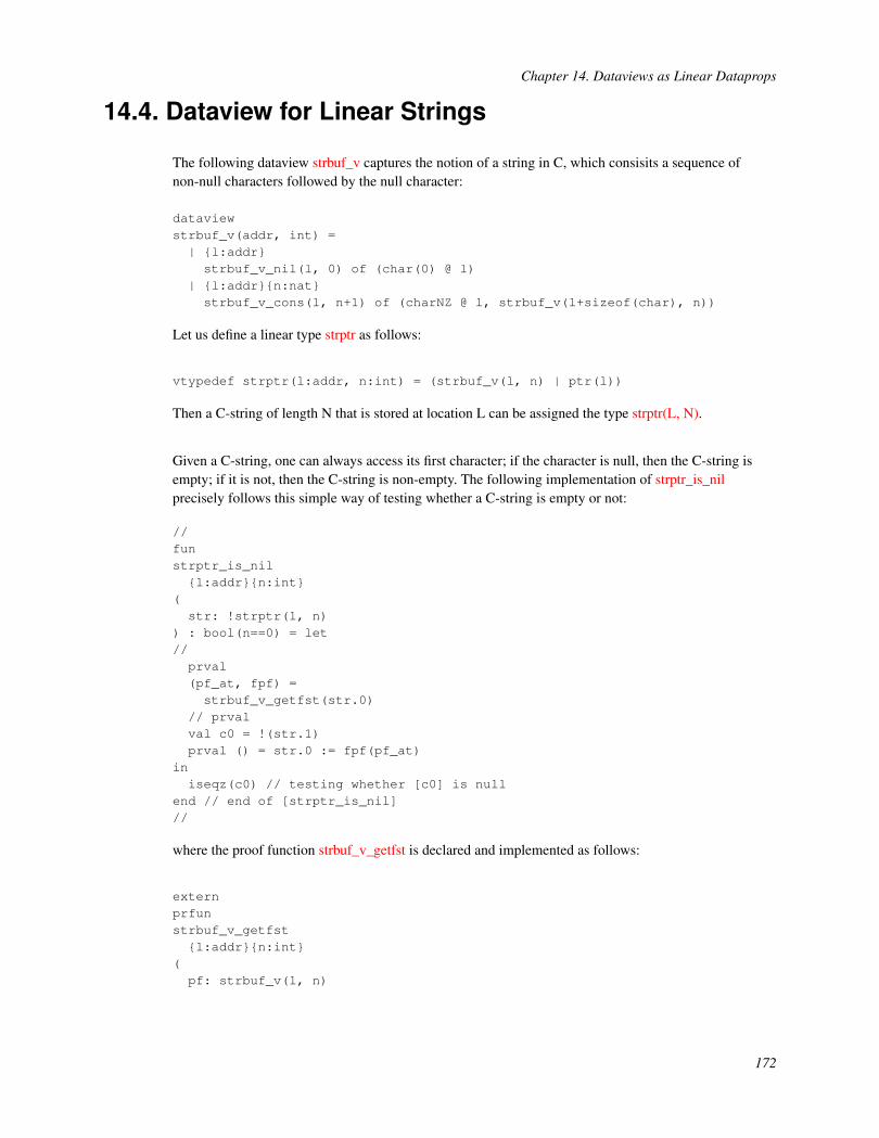
Chapter 14. Dataviews as Linear Dataprops
14.4. Dataview for Linear Strings
The following dataview strbuf_v captures the notion of a string in C, which consisits a sequence ofnon-null characters followed by the null character:
dataviewstrbuf_v(addr, int) =| {l:addr}strbuf_v_nil(l, 0) of (char(0) @ l)
| {l:addr}{n:nat}strbuf_v_cons(l, n+1) of (charNZ @ l, strbuf_v(l+sizeof(char), n))
Let us define a linear type strptr as follows:
vtypedef strptr(l:addr, n:int) = (strbuf_v(l, n) | ptr(l))
Then a C-string of length N that is stored at location L can be assigned the type strptr(L, N).
Given a C-string, one can always access its first character; if the character is null, then the C-string isempty; if it is not, then the C-string is non-empty. The following implementation of strptr_is_nilprecisely follows this simple way of testing whether a C-string is empty or not:
//funstrptr_is_nil{l:addr}{n:int}
(str: !strptr(l, n)
) : bool(n==0) = let//prval(pf_at, fpf) =strbuf_v_getfst(str.0)
// prvalval c0 = !(str.1)prval () = str.0 := fpf(pf_at)
iniseqz(c0) // testing whether [c0] is null
end // end of [strptr_is_nil]//
where the proof function strbuf_v_getfst is declared and implemented as follows:
externprfunstrbuf_v_getfst{l:addr}{n:int}
(pf: strbuf_v(l, n)
172

Chapter 14. Dataviews as Linear Dataprops
) : [c:int | (c==0 && n==0) || (c != 0 && n > 0)
] (char(c) @ l, char(c) @ l -<lin,prf> strbuf_v(l, n))
(* ****** ****** *)
primplmntstrbuf_v_getfst(pf) =
(case+ pf of| strbuf_v_nil(pf_at) => #[.. | (pf_at, llam(pf_at) => strbuf_v_nil(pf_at))]| strbuf_v_cons(pf_at, pf2) => #[.. | (pf_at, llam(pf_at) => strbuf_v_cons(pf_at, pf2))])
The following implementation gives another example of handling the dataview strbuf_v:
funstrptr_length{l:addr}{n:int}
(str: !strptr(l, n)
) : size_t(n) = let//funloop{l:addr}{i,j:int}(pf: !strbuf_v(l, i)
| p0: ptr(l), j: size_t(j)) : size_t(i+j) = let//prval[c:int](pf_at, fpf) = strbuf_v_getfst(pf)//val c0 = !p0//prval ((*return*)) = pf := fpf(pf_at)//in//ifiseqz(c0)then jelse res where{prvalstrbuf_v_cons(pf_at, pf2) = pf
173
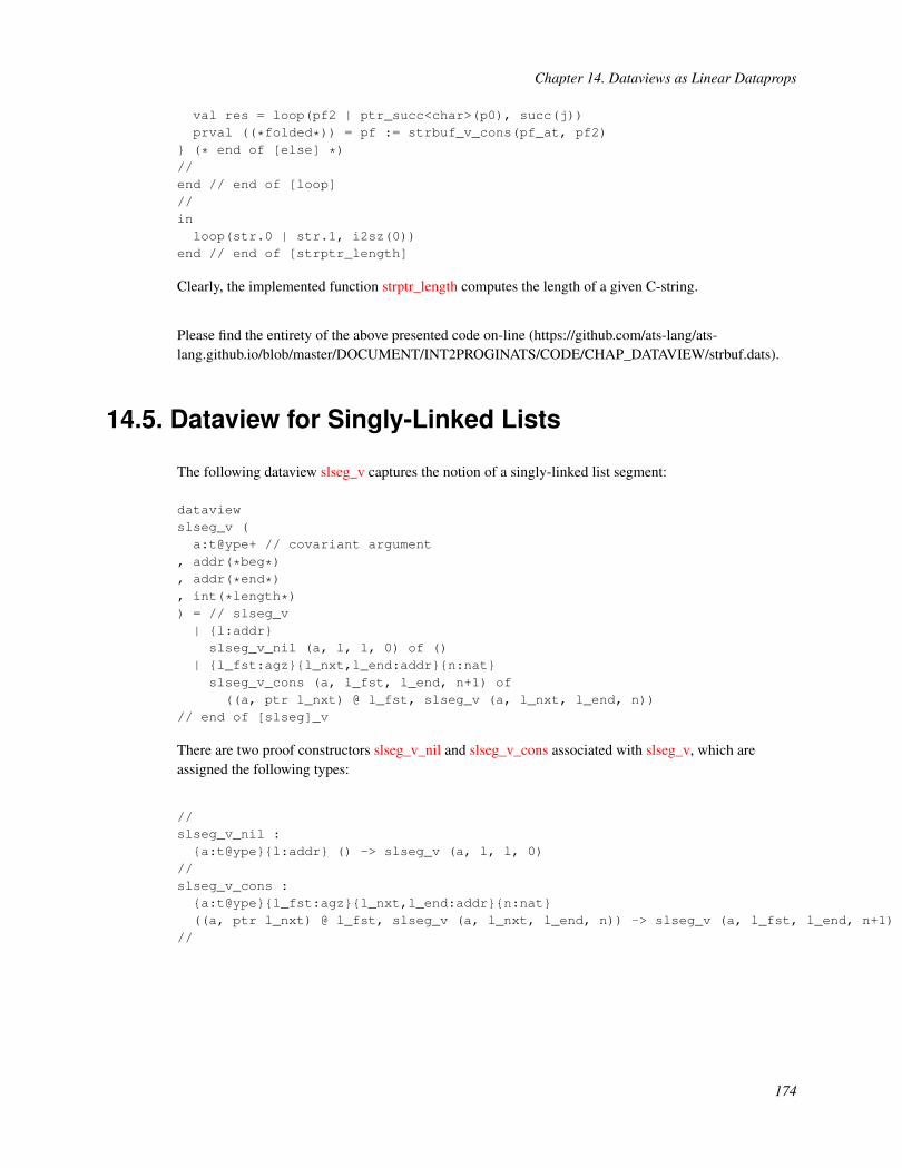
Chapter 14. Dataviews as Linear Dataprops
val res = loop(pf2 | ptr_succ<char>(p0), succ(j))prval ((*folded*)) = pf := strbuf_v_cons(pf_at, pf2)
} (* end of [else] *)//end // end of [loop]//inloop(str.0 | str.1, i2sz(0))
end // end of [strptr_length]
Clearly, the implemented function strptr_length computes the length of a given C-string.
Please find the entirety of the above presented code on-line (https://github.com/ats-lang/ats-lang.github.io/blob/master/DOCUMENT/INT2PROGINATS/CODE/CHAP_DATAVIEW/strbuf.dats).
14.5. Dataview for Singly-Linked Lists
The following dataview slseg_v captures the notion of a singly-linked list segment:
dataviewslseg_v (a:t@ype+ // covariant argument
, addr(*beg*), addr(*end*), int(*length*)) = // slseg_v| {l:addr}slseg_v_nil (a, l, l, 0) of ()
| {l_fst:agz}{l_nxt,l_end:addr}{n:nat}slseg_v_cons (a, l_fst, l_end, n+1) of((a, ptr l_nxt) @ l_fst, slseg_v (a, l_nxt, l_end, n))
// end of [slseg]_v
There are two proof constructors slseg_v_nil and slseg_v_cons associated with slseg_v, which areassigned the following types:
//slseg_v_nil :{a:t@ype}{l:addr} () -> slseg_v (a, l, l, 0)
//slseg_v_cons :{a:t@ype}{l_fst:agz}{l_nxt,l_end:addr}{n:nat}((a, ptr l_nxt) @ l_fst, slseg_v (a, l_nxt, l_end, n)) -> slseg_v (a, l_fst, l_end, n+1)
//
174

Chapter 14. Dataviews as Linear Dataprops
Note that agz is a subset sort for addresses that are not null. Given a type T, two addresses L1 and L2,and a natural number N, the view slseg_v(T, L1, L2, N) is for a singly-linked list segment containing Nelements of the type T that starts at L1 and finishes at L2. In the case where L2 is the null pointer, thenthe list segment is considered a list as is formally defined below:
viewdef slist_v(a:t@ype, l:addr, n:int) = slseg_v (a, l, null, n)
// end of [slist_v]
Given a type T, a pointer pointing to L plus a proof of the view slist_v(T, L, N) for some natural numberN is essentially the same as a pointer to a struct of the following declared type slist_struct in C:
typedefstruct slist {T data ; /* [T] matches the corresponding type in ATS */struct slist *next ; /* pointing to the tail of the list */
} slist_struct ;
Let us now see a simple example involving singly-linked lists:
fn{a:t@ype}slist_ptr_length{l:addr}{n:nat}
(pflst: !slist_v (a, l, n) | p: ptr l
) : int (n) = letfun loop{l:addr}{i,j:nat} .<i>.
(pflst: !slist_v (a, l, i) | p: ptr l, j: int (j)
) : int (i+j) =if p > 0 then letprval slseg_v_cons (pfat, pf1lst) = pflstval res = loop (pf1lst | !p.1, j+1) // !p.1 points to the tailprval () = pflst := slseg_v_cons (pfat, pf1lst)
inres
end else let // the length of a null list is 0prval slseg_v_nil () = pflst in pflst := slseg_v_nil (); j
end (* end of [if] *)// end of [loop]
inloop (pflst | p, 0)
end // end of [slist_ptr_length]
175

Chapter 14. Dataviews as Linear Dataprops
The function template slist_ptr_length computes the length of a given singly-linked list. Note that theinner function loop is tail-recursive. The above implementation of slist_ptr_length essentiallycorresponds to the following implementation in C:
intslist_ptr_length(slist_struct *p
) {int res = 0 ;while (p != NULL) { res = res + 1 ; p = p->next ; }return res ;
} // end of [slist_ptr_length]
As another example, the following function template slist_ptr_reverse turns a given linked list into itsreverse:
fn{a:t@ype}slist_ptr_reverse{l:addr}{n:nat}
(pflst: slist_v (a, l, n) | p: ptr l
) : [l:addr] (slist_v (a, l, n) | ptr l) = letfun loop{n1,n2:nat}{l1,l2:addr} .<n1>. (pf1lst: slist_v (a, l1, n1)
, pf2lst: slist_v (a, l2, n2)| p1: ptr l1, p2: ptr l2) : [l:addr] (slist_v (a, l, n1+n2) | ptr l) =if p1 > 0 then letprval slseg_v_cons (pf1at, pf1lst) = pf1lstval p1_nxt = !p1.1val () = !p1.1 := p2
inloop (pf1lst, slseg_v_cons (pf1at, pf2lst) | p1_nxt, p1)
end else letprval slseg_v_nil () = pf1lst in (pf2lst | p2)
end // end of [if]inloop (pflst, slseg_v_nil | p, the_null_ptr)
end // end of [slist_ptr_reverse]
By translating the tail-recursive function loop into a while-loop, we can readily turn the implementationof slist_ptr_reverse in ATS into the following implementation in C:
slist_struct*slist_ptr_reverse
176
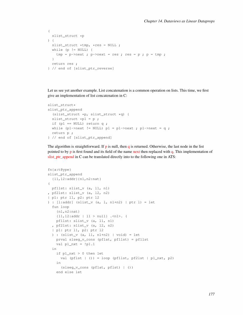
Chapter 14. Dataviews as Linear Dataprops
(slist_struct *p
) {slist_struct *tmp, *res = NULL ;while (p != NULL) {tmp = p->next ; p->next = res ; res = p ; p = tmp ;
}return res ;
} // end of [slist_ptr_reverse]
Let us see yet another example. List concatenation is a common operation on lists. This time, we firstgive an implementation of list concatenation in C:
slist_struct*slist_ptr_append(slist_struct *p, slist_struct *q) {slist_struct *p1 = p ;if (p1 == NULL) return q ;while (p1->next != NULL) p1 = p1->next ; p1->next = q ;return p ;
} // end of [slist_ptr_append]
The algorithm is straightforward. If p is null, then q is returned. Otherwise, the last node in the listpointed to by p is first found and its field of the name next then replaced with q. This implementation ofslist_ptr_append in C can be translated directly into to the following one in ATS:
fn{a:t@ype}slist_ptr_append{l1,l2:addr}{n1,n2:nat}
(pf1lst: slist_v (a, l1, n1)
, pf2lst: slist_v (a, l2, n2)| p1: ptr l1, p2: ptr l2) : [l:addr] (slist_v (a, l, n1+n2) | ptr l) = letfun loop{n1,n2:nat}{l1,l2:addr | l1 > null} .<n1>. (pf1lst: slist_v (a, l1, n1)
, pf2lst: slist_v (a, l2, n2)| p1: ptr l1, p2: ptr l2) : (slist_v (a, l1, n1+n2) | void) = letprval slseg_v_cons (pf1at, pf1lst) = pf1lstval p1_nxt = !p1.1
inif p1_nxt > 0 then letval (pflst | ()) = loop (pf1lst, pf2lst | p1_nxt, p2)
in(slseg_v_cons (pf1at, pflst) | ())
end else let
177

Chapter 14. Dataviews as Linear Dataprops
val () = !p1.1 := p2prval slseg_v_nil () = pf1lst
in(slseg_v_cons (pf1at, pf2lst) | ())
end (* end of [if] *)end // end of [loop]
inif p1 > 0 then letval (pflst | ()) = loop (pf1lst, pf2lst | p1, p2)
in(pflst | p1)
end else letprval slseg_v_nil () = pf1lst in (pf2lst | p2)
end (* end of [if] *)end // end of [slist_ptr_append]
In the above examples, it is evident that the code in ATS is a lot more verbose than its counterpart in C.However, the former is also a lot more robust than the latter in the following sense: If a minor change ismade to the code in ATS (e.g., renaming identifiers, reordering function arguments), it is most likely thata type-error is to be reported when the changed code is typechecked. On the other hand, the same thingcannot be said about the code written in C. For instance, the following erroneous implementation ofslist_ptr_reverse in C is certainly type-correct:
/*** This implementation is *incorrect* but type-correct:
*/slist_struct*slist_ptr_reverse(slist_struct *p)
{slist_struct *tmp, *res = NULL ;while (p != NULL) {tmp = p->next ; res = p ; p->next = res ; p = tmp ;
}return res ;
} // end of [slist_ptr_reverse]
I now point out that the dataview slseg_v is declared here in a manner that does not address the issue ofallocating and freeing list nodes, and it is done so for the sake of a less involved presentation. A dataviewfor singly-linked lists that does handle allocation and deallocation of list nodes can also be declared inATS, but there is really little need for it as we can declare a dataviewtype for such lists that is far moreconvenient to use. However, dataviews are fundamentally more general and flexible than dataviewtypes,and there are many common data structures (e.g. doubly-linked lists) that can only be properly handledwith dataviews in ATS.
178

Chapter 14. Dataviews as Linear Dataprops
14.6. Proof Functions for View-Changes
By the phrase view-change, I mean applying a function to proofs of a set of views to turn them intoproofs of another set of views. As this function itself is a proof function, there is no run-time costassociated with each view-change. For instance, a proof of the at-view int32@L for any address L can beturned into a proof of a tuple of 4 at-views: int8@L, int8@L+1, int8@L+2 and int8@L+3, where int32and int8 are types for 32-bit and 8-bit integers, respectively. Often more interesting view-changes involverecursively defined proof functions, and I present several of such cases in the rest of this section.
When implementing an array subscripting operation of O(1)-time, we need a proof function to changethe view of one array into the views of two adjacently located arrays and another proof function to doprecisely the opposite. Formally speaking, we need to construct the following two proof functionsarray_v_split and array_v_unsplit:
//prfunarray_v_split{a:t@ype}{l:addr}{n,i:nat | i <= n}
(pfarr: array_v (a, l, n)
) : (array_v (a, i, l), array_v (a, n-i, l+i*sizeof(a)))//prfunarray_v_unsplit{a:t@ype}{l:addr}{n1,n2:nat}
(pf1arr: array_v (a, l, n1), pf2arr: array_v (a, l+n1*sizeof(a), n2)
) : array_v (a, l, n1+n2)//
An implementation of array_v_split is given as follows:
primplmntarray_v_split{a}{l}{n,i}(pfarr) = letprfun split{l:addr}{n,i:nat | i <= n} .<i>.
(pfarr: array_v (a, l, n)
) : (array_v (a, l, i)
, array_v (a, l+i*sizeof(a), n-i)) =sif i > 0 then letprval array_v_cons (pf1, pf2arr) = pfarrprval (pf1res1, pf1res2) = split{..}{n-1,i-1} (pf2arr)
in
179

Chapter 14. Dataviews as Linear Dataprops
(array_v_cons (pf1, pf1res1), pf1res2)end else letprval EQINT () = eqint_make{i,0}((*void*))
in(array_v_nil (), pfarr)
end // end of [sif]insplit (pfarr)
end // end of [array_v_split]
Note that the keyword primplmnt (instead of implement) should be used for implementing prooffunctions. One can also choose to use the keyword primplement in place of primplmnt. Clearly, the prooffunction split directly encodes a proof based on mathematical induction. Following is an implementationof array_v_unsplit:
primplmntarray_v_unsplit{a}{l}{n1,n2}(pf1arr, pf2arr) = letprfun unsplit{l:addr}{n1,n2:nat} .<n1>.
(pf1arr: array_v (a, l, n1)
, pf2arr: array_v (a, l+n1*sizeof(a), n2)) : array_v (a, l, n1+n2) =sif n1 > 0 then letprvalarray_v_cons (pf1, pf1arr) = pf1arrprval pfres = unsplit (pf1arr, pf2arr)
inarray_v_cons (pf1, pfres)
end else letprval array_v_nil () = pf1arr in pf2arr
end // end of [sif]inunsplit (pf1arr, pf2arr)
end // end of [array_v_unsplit]
The proof function unsplit also directly encodes a proof based on mathematical induction.
Let us now see an even more interesting proof function for performing view-change. The interface of theproof function array_v_takeout is given as follows:
//prfunarray_v_takeout{a:t@ype}{l:addr}{n,i:nat | i < n}
(pfarr: array_v (a, l, n)
180

Chapter 14. Dataviews as Linear Dataprops
) : (a @ l+i*sizeof(a), a @ l+i*sizeof(a) -<lin,prf> array_v (a, l, n))//
Note that the following type is for a linear proof function that takes a proof of an at-view to return aproof of an array-view:
a @ l+i*sizeof(a) -<lin,prf> array_v (a, l, n)
As such a function essentially represents an array with one missing cell, we may simply say thatarray_v_takeout turns the view of an array into an at-view (for one cell) and a view for the rest of thearray. By making use of array_v_takeout, we can give another implementation of arrget:
implement{a}(*tmp*)arrget{l}{n,i}(pf | p, i) = x where {prval (pf1, fpf2) =array_v_takeout{a}{l}{n,i} (pf)val x = ptr_get1<a> (pf1 | ptr_add<a> (p, i))prval () = pf := fpf2 (pf1) // putting the cell and the rest together
} (* end of [arrget] *)
The proof function array_v_takeout can be implemented as follows:
primplmntarray_v_takeout{a}{l}{n,i}(pfarr) = letprfun takeout{l:addr}{n,i:nat | i < n} .<i>.
(pfarr: array_v (a, l, n)
) : (a @ l+i*sizeof(a)
, a @ l+i*sizeof(a) -<lin,prf> array_v (a, l, n)) = letprval array_v_cons (pf1at, pf1arr) = pfarr
insif i > 0 then letprval (pfres, fpfres) = takeout{..}{n-1,i-1}(pf1arr)
in(pfres, llam (pfres) => array_v_cons (pf1at, fpfres (pfres)))
end else letprval EQINT () = eqint_make{i,0}((*void*))
in(pf1at, llam (pf1at) => array_v_cons (pf1at, pf1arr))
end // end of [sif]end // end of [takeout]
in
181

Chapter 14. Dataviews as Linear Dataprops
takeout{l}{n,i}(pfarr)end // end of [array_v_takeout]
Note that llam is a keyword for forming linear functons. Once a linear function is applied, it is consumedand the resource in it, if not reclaimed, moves into the result it returns.
The proof functions presented so far for view-changes are all manipulating array-views. The followingone is different in this regard as it combines two views for singly-linked list segments into one:
//prfunslseg_v_unsplit{a:t@ype}{l1,l2,l3:addr}{n1,n2:nat}
(pf1lst: slseg_v (a, l1, l2, n1), pf2lst: slseg_v (a, l2, l3, n2)
) : slseg_v (a, l1, l3, n1+n2)//
The type of slseg_v_unsplit essentially states that a list segment from L1 to L2 that is of length N1 andanother list segment from L2 to L3 that is of length N2 can be thought of as a list segment from L1 to L3that is of length N1+N2. The following implementation of slseg_v_unsplit is largely parallel to that ofarray_v_unsplit:
primplmntslseg_v_unsplit{a}(pf1lst, pf2lst) = letprfun unsplit{l1,l2,l3:addr}{n1,n2:nat} .<n1>.
(pf1lst: slseg_v (a, l1, l2, n1), pf2lst: slseg_v (a, l2, l3, n2)
) : slseg_v (a, l1, l3, n1+n2) =sif n1 > 0 then letprval slseg_v_cons (pf1at, pf1lst) = pf1lst
inslseg_v_cons (pf1at, unsplit (pf1lst, pf2lst))
end else letprval slseg_v_nil () = pf1lst in pf2lst
end // end of [sif]inunsplit (pf1lst, pf2lst)
end // end of [slseg_v_unsplit]
The reader may find it interesting to give an implementation of slist_ptr_append by making use ofslseg_v_unsplit.
182

Chapter 14. Dataviews as Linear Dataprops
Please find on-line the files array.dats (https://github.com/ats-lang/ats-lang.github.io/blob/master/DOCUMENT/INT2PROGINATS/CODE/CHAP_DATAVIEW/array.dats) andslist.dats (https://github.com/ats-lang/ats-lang.github.io/blob/master/DOCUMENT/INT2PROGINATS/CODE/CHAP_DATAVIEW/slist.dats),which contains the code employed for illustration in this section.
183

Chapter 15. Dataviewtypes as Linear Datatypes
A dataviewtype can be thought of as a linear version of datatype. To a large extent, it is a combination ofa datatype and a dataview. This programming feature is primarily introduced into ATS for the purpose ofproviding in the setting of manual memory management the kind of convenience brought by patternmatching. In a situation where GC must be reduced or even completely eliminated, dataviewtypes canoften be chosen as a replacement for datatypes. I now present in this chapter some commonlyencountered dataviewtypes and their uses.
15.1. Linear Optional Values
When an optional value is created, the value is most likely to be used immediately and then discarded. Ifsuch a value is assigned a linear type, then the memory allocated for storing it can be efficientlyreclaimed. The dataviewtype option_vt for linear optional values is declared as follows:
//datavtypeoption_vt (a:t@ype+, bool) =| Some_vt (a, true) of a | None_vt (a, false) of ()
// end of [option_vt]//vtypedef Option_vt (a:t@ype) = [b:bool] option_vt(a, b)//
Note that datavtype is just the short version of dataviewtype. The introduced dataviewtype option_vt iscovariant in its first argument and there are two data constructors Some_vt and None_vt associated withit. In the following example, find_rightmost tries to find the rightmost element in a list that satisfies agiven predicate:
fun{a:t@ype}find_rightmost{n:nat} .<n>.
(xs: list (a, n), P: (a) -<cloref1> bool
) : Option_vt (a) =(case+ xs of| list_cons (x, xs) => let
val opt = find_rightmost (xs, P)incase opt of| ~None_vt () => if P (x) then Some_vt (x) else None_vt ()| _ (*Some_vt*) => opt
end // end of [list_cons]| list_nil () => None_vt ()
) (* end of [find_rightmost] *)
184

Chapter 15. Dataviewtypes as Linear Datatypes
Note that the tilde symbol (~) in front of the pattern None_vt() indicates that the memory for the nodethat matches the pattern is freed before the body of the matched clause is evaluated. In this case, nomemory is actually freed as None_vt is mapped to the null pointer. I will soon give more detailedexplanation about freeing memory allocated for constructors associated with dataviewtypes.
As another example, the following function template list_optcons tries to construct a new list with itshead element extracted from a given optional value:
fn{a:t@ype}list_optcons{b:bool}{n:nat}
(opt: option_vt (a, b), xs: list (a, n)
) : list (a, n+bool2int(b)) =case+ opt of| ~Some_vt (x) => list_cons (x, xs) | ~None_vt () => xs
// end of [list_optcons]
The symbol bool2int stands for a built-in static function in ATS that maps true and false to 1 and 0,respectively. What is special here is that the first argument of list_optcons, which is linear, is consumedafter a call to list_optcons returns and the memory it occupies is reclaimed.
15.2. Linear Lists
A linear list is essentially the same as a singly-linked list depicted by the dataview slist_v. However,memory allocation and deallocation of list-nodes not handled previously are handled this time. Thefollowing declaration introduces a linear datatype list_vt, which forms a boxed type (of the sortviewtype) when applied to a type and an integer:
datavtypelist_vt (a:t@ype+, int) =| list_vt_nil (a, 0) of ()| {n:nat}list_vt_cons (a, n+1) of (a, list_vt (a, n))
// end of [list_vt]
Given a type T and an integer I, list_vt(T, I) is for linear lists of length I in which each element is of thetype T.
Assume that a data constructor named foo is associated with a dataviewtype. Then there is acorresponding viewtype construtor of the name foo_unfold that takes n+1 addresses to form a viewtype,where n is the arity of foo. For instance, there is a viewtype constructor list_vt_cons_unfold that takes 3address L0, L1 and L2 to form a viewtype list_vt_cons_unfold(L0, L1, L2). This viewtype is for alist-node created by a call to list_vt_cons such that the node is located at L0 and the two arguments oflist_vt_cons are located at L1 and L2 while the proofs for the at-views associated with L1 and L2 are putin the store for currently available proofs.
185

Chapter 15. Dataviewtypes as Linear Datatypes
The following function template length computes the length of a given linear list:
fn{a:t@ype} length{n:nat}(xs: !list_vt (a, n)): int n = letfun loop{i,j:nat | i+j==n} .<i>.(xs: !list_vt (a, i), j: int j): int (n) =case+ xs of| list_vt_cons (_, xs1) => loop (xs1, j+1) | list_vt_nil () => j
// end of [loop]inloop (xs, 0)
end // end of [length]
The interface of length indicates that length<T> returns an integer equal to I when applied to a list of thetype list_vt(T, I), where T and I are a type and an integer, respectively. Note that the symbol ! in front ofthe type of a function argument indicates that the argument is call-by-value and it is preserved after a callto the function. The function loop inside the body of length is tail-recursive. Given a linear list and aninteger, loop returns the sum of the length of the list and the integer. In the body of loop, if xs matchesthe pattern list_vt_cons(_, xs1), then the name xs1 is bound to the tail of xs. Note that xs1 is a value(instead of a variable), and it is not allowed that xs1 be modified into another value (of a different type).
Suppose that we do want to modify the content stored in a list-node. For instance, we may want todouble the value of each integer stores in a linear integer list. The following code implements a functionnamed list_vt_2x that does precisely this:
funlist_vt_2x{n:nat}(xs: !list_vt (int, n) >> _): void =
(case+ xs of| @list_vt_cons
(x, xs1) => letval () = x := 2 * xval () = list_vt_2x (xs1)prval () = fold@ (xs)
in// nothing
end // end of [list_vt_cons]| list_vt_nil () => ()
) (* end of [list_vt_2x] *)
Given a type T, the notation (!T >> _) is a shorthand for (!T >> T). Note that the special symbol @ infront of the pattern list_vt_cons(x, xs1) means unfolding. If xs matches this pattern, then x and xs1 arebound to the pointers pointing to some memory locations L1 and L2 where the head and tail of xs arestored, respectively, and the type of xs changes into list_vt_cons_unfold(L0, L1, L2) for L0 being thelocation of the list-node referred to by xs. In the body of the clause guarded by the pattern list_vt_cons(x,xs1), x and xs1 are treated as variables (which are a form of left-value). The special proof function fold@is called on xs to fold it plus the proofs of at-views attached to L1 and L2 into a linear list.
186

Chapter 15. Dataviewtypes as Linear Datatypes
Let us now see an example where linear list-nodes are explicitly freed:
fun{a:t@ype} list_vt_free{n:nat} .<n>.(xs: list_vt (a, n)): void =
(case+ xs of| ~list_vt_cons
(x, xs1) => list_vt_free (xs1)| ~list_vt_nil ((*void*)) => ()
) (* end of [list_vt_free] *)
Given a linear list, the function list_vt_free frees all the nodes in the list. Let us go over the body oflist_vt_free carefully. If xs matches the pattern list_vt_cons(x, xs1), then the names x and xs1 are boundto the head and tail of xs, respectively; the special symbol ~ in front of the pattern indicates that thelist-node referred to by xs is freed immediately after xs matches the pattern. If xs matches the patternlist_vt_nil(), no bindings are generated; the special symbol ~ in front of the pattern indicates that thelist-node referred to by xs is freed; nothing in this case is actually freed at run-time as list_vt_nil ismapped to the null pointer.
It is also possible to use the special function free@ to explicitly free a node (also called a skeleton) left ina linear variable after the variable matches a pattern formed with a constructor associated with somedataviewtype. For instance, the following code gives another implementation of list_vt_free:
fun{a:t@ype} list_vt_free{n:nat} .<n>. (xs: list_vt (a, n)): void =case+ xs of| @list_vt_cons
(x, xs1) => letval xs1_ = xs1 // [xs1_] is the value stored in [xs1]val ((*void*)) = free@{a}{0}(xs) in list_vt_free (xs1_)
end // end of [list_vt_cons]| @list_vt_nil () => free@{a} (xs)
// end of [list_vt_free]
As it can be a bit tricky to use free@ in practice, I present more details as follows. First, let us note thatthe constructors list_vt_nil and list_vt_cons associated with list_vt are assigned the following types:
list_vt_nil : // one quantifier{a:t@ype} () -> list_vt (a, 0)
list_vt_cons : // two quantifiers{a:t@ype}{n:nat} (a, list_vt (a, n)) -> list_vt (a, n+1)
If free@ is applied to a node of the type list_vt_nil(), it needs one static argument, which is a type, toinstantiate the quantifier in the type of the constructor list_vt_nil. If free@ is applied to a node of the type
187

Chapter 15. Dataviewtypes as Linear Datatypes
list_vt_cons_unfold(L0, L1, L2), then it needs two static arguments, which are a type and an integer, toinstantiate the two quantifiers in the type of the constructor list_vt_cons. In the case where the type of xsis list_vt_cons_unfold(L0, L1, L2), typechecking the call free@{a}{0}(xs) implicitly consumes a proofof the at-view a?@L1 and another proof of the at-view list_vt(a, 0)?@L2. As there is no differencebetween list_vt(T, 0)? and list_vt(T, I)? for any T and I, the static argument 0 is chosen in the code. As amatter of fact, any natural number can be used in place of 0 as the second static argument of free@.
15.2.1. Linear List-Reversing
The following code implements a function reverse that turns a given linear list into its reverse:
fn{a:t@ype} reverse{n:nat}(xs: list_vt (a, n)
) : list_vt (a, n) = letfun revapp{i,j:nat | i+j==n} .<i>.
(xs: list_vt (a, i), ys: list_vt (a, j)
) : list_vt (a, n) =case+ xs of| @list_vt_cons
(_, xs1) => letval xs1_ = xs1val () = xs1 := ysprval () = fold@ (xs)
inrevapp (xs1_, xs)
end // end of [list_vt_cons]| ~list_vt_nil ((*void*)) => ys
// end of [revapp]inrevapp (xs, list_vt_nil)
end // end of [reverse]
The type assigned to reverse indicates that the function returns a linear list of the same length as the oneit consumes. Note that the inner function revapp is tail-recursive. This implementation of linearlist-reversing directly corresponds to the one presented previously that is based the dataview slseg_v (forsingly-linked list segments). Comparing the two implementations, we can see that the one based ondataviewtype is significantly simplified at the level of types. For instance, there is no explicit mentioningof pointers in the types assigned to functions reverse and revapp.
188

Chapter 15. Dataviewtypes as Linear Datatypes
15.2.2. Linear List-Appending
The following code implements a function append that concatenates two given linear lists into one:
fn{a:t@ype} append{m,n:nat}(xs: list_vt (a, m)
, ys: list_vt (a, n)) : list_vt (a, m+n) = letfun loop {m,n:nat} .<m>. // [loop] is tail-recursive(xs: &list_vt (a, m) >> list_vt (a, m+n), ys: list_vt (a, n)
) : void =case+ xs of| @list_vt_cons
(_, xs1) => letval () = loop (xs1, ys) in fold@ (xs)
end // end of [list_vt_cons]| ~list_vt_nil ((*void*)) => xs := ys
// end of [loop]var xs: List_vt (a) = xs // creating a left-value for [xs]val () = loop (xs, ys)
inxs
end // end of [append]
As the call fold@(xs) in the body of the function loop is erased after typechecking, loop is atail-recursive function. Therefore, append can be called on lists of any length without the concern ofpossible stack overflow. The type for the first argument of loop begins with the symbol &, whichindicates that this argument is call-by-reference. The type of loop simply means that its first argument ischanged from a list of length m into a list of length m+n while its second argument is consumed.
This implementation of list append essentially corresponds to the one presented previously that is basedon the dataview slseg_v. Comparing these two, we can easily see that the above one is much simpler andcleaner, demonstrating concretely some advantage of dataviewtypes over dataviews.
This is also a good place for me to mention a closely related issue involving (functional) list constructionand tail-recursion. Following is a typical implementation of functioal list concatenation:
fun{a:t@ype} append1{m,n:nat}(xs: list(a, m), ys: list(a, n)
) : list (a, m+n) =case+ xs of| list_nil() => ys| list_cons(x, xs) => list_cons(x, append1<a>(xs, ys))
189

Chapter 15. Dataviewtypes as Linear Datatypes
// end of [append1]
Clearly, append1 is not tail-recursive, which means that it may cause stack overflow at run-time if its firstargument is very long (e.g., containing 1 million elements). There is, however, a direct and type-safe wayin ATS to implement functional list concatenation in a tail-recursive manner, thus eliminating theconcern of potential stack overflow. For instance, the following implementation of append2 returns theconcatenation of two given functional lists while being tail-recursive:
fun{a:t@ype} append2{m,n:nat}(xs: list (a, m), ys: list (a, n)
) : list (a, m+n) = let//fun loop{m,n:nat} .<m>.
(xs: list (a, m), ys: list (a, n)
, res: &(List a)? >> list (a, m+n)) : void =(case+ xs of| list_nil() =>
(res := ys)// end of [list_nil]
| list_cons(x, xs) => letval () =res := list_cons{a}{0}(x, _)val+ list_cons (_, res1) = resval () = loop (xs, ys, res1)prval ((*void*)) = fold@ (res)
in// nothing
end // end of [list_cons]) (* end of [loop] *)//var res: List(a)val () = loop (xs, ys, res)//inres
end // end of [append2]
During typechecking, the expression list_cons{a}{0}(x, _) is assigned the (linear) typelist_cons_unfold(L0, L1, L2) for some addresses L0, L1 and L2 while a proof of the at-view a@L1 andanother proof of the at-view list(a, 0)?@L2 are put into the store for currently available proofs. Note thatthe special symbol _ simply indicates that the tail of the newly constructed list is uninitialized. A partiallyinitialized list of the type list_cons_unfold(L0, L1, L2) is guaranteed to match the pattern list_cons(_,res1), yielding a binding between res1 and the pointer pointing to L2 where the (possibly uninitialized)tail of the list is stored. When fold@ is called on a variable of the type list_cons_unfold(L0, L1, L2), it
190

Chapter 15. Dataviewtypes as Linear Datatypes
changes the type of the variable to list(T, N+1) by consuming a proof of the at-view T@L1 and anotherproof of the at-view list(T, N)@L2, where T and N are a type and an integer, respectively.
15.2.3. Summary
With dataviewtypes, we can largely retain the convenience of pattern matching associated with datatypeswhile supporting explicit memory management. Compared to dataviews, dataviewtypes are less general.However, if a dataviewtype can be employed to solve a problem, then the solution is often significantlysimpler and cleaner than an alternative dataview-based one.
15.3. Example: Merge-Sort on Linear Lists
When merge-sort is employed to sort an array of elements, it requires additional memory proportionateto the size of the array in order to move the elements around, which is considered a significant weaknessof merge-sort. However, merge-sort does not have this requirement when it operates on a linear list. Ipresent as follows an implementation of merge-sort on linear lists that can readily rival its counterpart inC in terms of both time-efficiency and memory-efficiency. The invariants captured in this implementationand the easiness to capture them should provide strong evidence that attests to ATS being a programminglanguage capable of enforcing great precision in practical programming.
Let us first introduce a type definition and an interface for a function template that compares elements inlists to be sorted:
//typedef cmp (a:t@ype) = (&a, &a) -> int//fun{a:t@ype}compare (x: &a, y: &a, cmp: cmp(a)): int//
The interface for merge-sort is given as follows:
fun{a:t@ype} mergeSort{n:nat}(xs: list_vt (a, n), cmp: cmp a): list_vt (a, n)
// end of [mergeSort]
The first argument of mergeSort is a linear list (to be sorted) and the second one a function for comparingthe elements in the linear list. Clearly, the interface of mergeSort indicates that mergeSort consumes itsfirst argument and then returns a linear list that is of the same length as its first argument. As is tobecome clear, the returned linear list is constructed with the nodes of the consumed one. In particular, theimplementation of mergeSort given as follows does not involve any memory allocation or deallocation.
191

Chapter 15. Dataviewtypes as Linear Datatypes
The function template for merging two sorted lists into one is given as follows:
fun{a:t@ype} merge{m,n:nat} .<m+n>.(xs: list_vt (a, m), ys: list_vt (a, n)
, res: &List_vt(a)? >> list_vt (a, m+n), cmp: cmp a) : void =case+ xs of| @list_vt_cons (x, xs1) => (case+ ys of| @list_vt_cons (y, ys1) => let
val sgn = compare<a> (x, y, cmp)inif sgn <= 0 then let // stable sortingval () = res := xsval xs1_ = xs1prval () = fold@ (ys)val () = merge<a> (xs1_, ys, xs1, cmp)
infold@ (res)
end else letval () = res := ysval ys1_ = ys1prval () = fold@ (xs)val () = merge<a> (xs, ys1_, ys1, cmp)
infold@ (res)
end // end of [if]end (* end of [list_vt_cons] *)
| ~list_vt_nil () => (fold@ (xs); res := xs)) // end of [list_vt_cons]
| ~list_vt_nil () => (res := ys)// end of [merge]
Unlike the one given in a previous functional implementation, this implementation of merge istail-recursive and thus is guaranteed to be translated into a loop in C by the ATS compiler. This meansthat the concern of merge being unable to handle very long lists (e.g., containing 1 million elements) dueto potential stack overflow is eliminated.
The next function template is for splitting a given linear lists into two:
fun{a:t@ype} split{n,k:nat | k <= n} .<n-k>.(xs: &list_vt (a, n) >> list_vt (a, n-k), nk: int (n-k)
) : list_vt (a, k) =if nk > 0 then letval+@list_vt_cons(_, xs1) = xs
192

Chapter 15. Dataviewtypes as Linear Datatypes
val res = split<a> (xs1, nk-1); prval () = fold@(xs)inres
end else letval res = xs; val () = xs := list_vt_nil () in res
end // end of [if]// end of [split]
Note that the implementation of split is also tail-recursive.
The following function template msort takes a linear list, its length and a comparsion function, and itreturns a sorted version of the given linear list:
fun{a:t@ype} msort{n:nat} .<n>.(xs: list_vt (a, n), n: int n, cmp: cmp(a)
) : list_vt (a, n) =if n >= 2 then letval n2 = half(n)val n3 = n - n2var xs = xs // lvalue for [xs]val ys = split<a> (xs(*cbr*), n3)val xs = msort<a> (xs, n3, cmp)val ys = msort<a> (ys, n2, cmp)var res: List_vt (a) // uninitializedval () = merge<a> (xs, ys, res(*cbr*), cmp)
inres
end else xs// end of [msort]
The second argument of msort is passed so that the length of the list being sorted does not have to becomputed directly by traversing the list when each recursive call to msort is made.
Finally, mergeSort can be implemented with a call to msort:
implement{a}mergeSort (xs, cmp) = msort<a> (xs, length (xs), cmp)
By inspecting the implementation of split and merge, we can readiy see that mergeSort performs stablesorting, that is, it preserves the order of equal elements during sorting.
Please find on-line (https://github.com/ats-lang/ats-lang.github.io/blob/master/DOCUMENT/INT2PROGINATS/CODE/CHAP_DATAVTYPE/mergeSort.dats)the entirety of the code presented in this section plus some additional code for testing.
193

Chapter 15. Dataviewtypes as Linear Datatypes
15.4. Example: Insertion Sort on Linear Lists
I present a standard implementation of insertion sort on linear lists in this section. The interface forinsertion sort is given as follows:
fun{a:t@ype} insertionSort{n:nat}(xs: list_vt (a, n), cmp: cmp a): list_vt (a, n)
// end of [insertionSort]
Like mergeSort, insertionSort is implemented in a manner that makes no use of memory allocation ordeallocation. Given a linear list, insertionSort essentially shuffles the nodes in the list to form a sorted list.
The following code implements a function insord that inserts a given list-node into a sorted linear list toform another sorted linear list:
fun{a:t@ype} insord{l0,l1,l2:addr}{n:nat}
(pf1: a @ l1
, pf2: list_vt (a, 0)? @ l2| xs0: &list_vt (a, n) >> list_vt (a, n+1), nx0: list_vt_cons_unfold (l0, l1, l2), p1: ptr (l1), p2: ptr (l2), cmp: cmp (a)) : void =(case+ xs0 of| @list_vt_cons
(x0, xs1) => letval sgn = compare<a> (x0, !p1, cmp)
inif sgn <= 0 // HX: for stableness: [<=] instead of [<]then letval () = insord<a> (pf1, pf2 | xs1, nx0, p1, p2, cmp)prval () = fold@ (xs0)
in// nothing
end // end of [then]else letprval () = fold@ (xs0)val () = (!p2 := xs0; xs0 := nx0)prval () = fold@ (xs0)
in// nothing
end // end of [else]// end of [if]
end // end of [list_vt_cons]| ~list_vt_nil () =>
194

Chapter 15. Dataviewtypes as Linear Datatypes
{val () = xs0 := nx0val () = !p2 := list_vt_nil ()prval () = fold@ (xs0)
}) (* end of [insord] *)
The implementation of insord is tail-recursive. The type assigned to insord indicates that the argumentxs0 of insord is call-by-reference. If xs0 stores a list of length n when insord is called, then it stores a listof length n+1 when insord returns. The arguments nx0, p1 and p2 are call-by-value, and they should bebound to a list-node and the first and second fields in the list-node, respectively, when a call to insordinitiates. The proof arguments pf1 and pf2 are needed so that the pointers bound to p1 and p2 can beaccessed and updated.
The function template insertionSort can now be readily implemented based insord:
implement{a}insertionSort(xs, cmp) = let
//fun loop{m,n:nat}(xs: list_vt (a, m)
, ys: &list_vt (a, n) >> list_vt (a, m+n), cmp: cmp (a)) : void =case+ xs of| @list_vt_cons
(x, xs1) => letval xs1_ = xs1val ((*void*)) =insord<a> (view@x, view@xs1 | ys, xs, addr@x, addr@xs1, cmp)
// end of [va]inloop (xs1_, ys, cmp)
end // end of [list_vt_cons]| ~list_vt_nil ((*void*)) => ()
//var ys = list_vt_nil{a}()val () = loop (xs, ys, cmp)//inys
end // end of [insertionSort]
Clearly, this implementation of insertionSort is tail-recursive. While insertion sort is of O(n^2)-timecomplexity, it is often more efficient than merge-sort or quick-sort when sorting very short lists. Forinstance, we may implement msort (which is called by mergeSort) as follows by taking advantage of theefficiency of insertionSort on short lists:
fun{
195
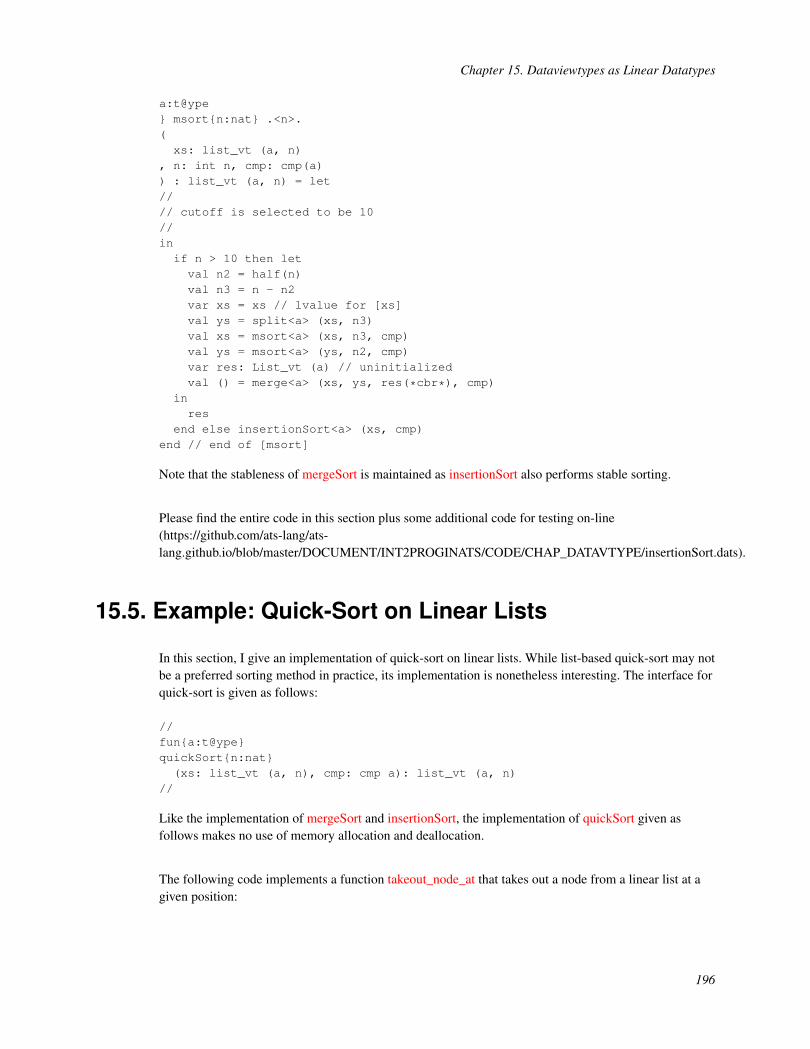
Chapter 15. Dataviewtypes as Linear Datatypes
a:t@ype} msort{n:nat} .<n>.(xs: list_vt (a, n)
, n: int n, cmp: cmp(a)) : list_vt (a, n) = let//// cutoff is selected to be 10//inif n > 10 then letval n2 = half(n)val n3 = n - n2var xs = xs // lvalue for [xs]val ys = split<a> (xs, n3)val xs = msort<a> (xs, n3, cmp)val ys = msort<a> (ys, n2, cmp)var res: List_vt (a) // uninitializedval () = merge<a> (xs, ys, res(*cbr*), cmp)
inres
end else insertionSort<a> (xs, cmp)end // end of [msort]
Note that the stableness of mergeSort is maintained as insertionSort also performs stable sorting.
Please find the entire code in this section plus some additional code for testing on-line(https://github.com/ats-lang/ats-lang.github.io/blob/master/DOCUMENT/INT2PROGINATS/CODE/CHAP_DATAVTYPE/insertionSort.dats).
15.5. Example: Quick-Sort on Linear Lists
In this section, I give an implementation of quick-sort on linear lists. While list-based quick-sort may notbe a preferred sorting method in practice, its implementation is nonetheless interesting. The interface forquick-sort is given as follows:
//fun{a:t@ype}quickSort{n:nat}(xs: list_vt (a, n), cmp: cmp a): list_vt (a, n)
//
Like the implementation of mergeSort and insertionSort, the implementation of quickSort given asfollows makes no use of memory allocation and deallocation.
The following code implements a function takeout_node_at that takes out a node from a linear list at agiven position:
196

Chapter 15. Dataviewtypes as Linear Datatypes
fun{a:t@ype}takeout_node_at{n:int}{k:nat | k < n}
(xs: &list_vt (a, n) >> list_vt (a, n-1), k: int(k)
) : list_vt_cons_pstruct (a, ptr?) =(//if k > 0 then letval+@list_vt_cons (x, xs1) = xsval res = takeout_node_at<a> (xs1, k-1)prval () = fold@ (xs)
inres
end else letval+@list_vt_cons (x, xs1) = xsval nx = xsval () = xs := xs1
in$UNSAFE.castvwtp0 ((view@x, view@xs1 | nx)) // HX: this is a safe cast
end // end of [if]//) (* end of [takeout_node_at] *)
Assume that a data constructor named foo is associated with a dataviewtype. Then there is acorresponding viewtype construtor of the name foo_pstruct that takes n types to form a viewtype, wheren is the arity of foo. For instance, there is a viewtype constructor list_vt_cons_pstruct that takes 2 typesT1 and T2 to form a viewtype list_vt_cons_pstruct(T1, T2). This viewtype is for a list-node created by acall to list_vt_cons such that the two arguments of list_vt_cons are of types T1 and T2. Essentially,list_vt_cons_pstruct(T1, T2) stands for list_vt_cons_unfold(L0, L1, L2) for some addresses L0, L1 andL2 plus two views T1@L1 and T2@L2.
A key step in quick-sort lies in partitioning a linear list based on a given pivot. This step is fulfilled bythe following code that implements a function template named partition:
fun{a:t@ype} partition{n,r1,r2:nat}(xs: list_vt (a, n), pvt: &a
, r1: int(r1), res1: list_vt (a, r1), res2: list_vt (a, r2), cmp: cmp (a)) : [n1,n2:nat | n1+n2==n+r1+r2](int(n1), list_vt (a, n1), list_vt (a, n2)) =
(case+ xs of| @list_vt_cons
(x, xs_tail) => letval xs_tail_ = xs_tailval sgn = compare<a> (x, pvt, cmp)
in
197

Chapter 15. Dataviewtypes as Linear Datatypes
if sgn <= 0 then letval r1 = r1 + 1val () = xs_tail := res1prval () = fold@ (xs)
inpartition<a> (xs_tail_, pvt, r1, xs, res2, cmp)
end else letval () = xs_tail := res2prval () = fold@ (xs)
inpartition<a> (xs_tail_, pvt, r1, res1, xs, cmp)
end // end of [if]end (* end of [list_vt_cons] *)
| ~list_vt_nil ((*void*)) => (r1, res1, res2)) (* end of [partition] *)
The implementation of partition is tail-recursive. Given a linear list and a pivot, partition returns a tuple(r1, res1, res2) such that res1 contains every element in the list that is less than or equal to the pivot, res2contains the rest, and r1 is the length of res1. The way in which the nodes of the given linear list aremoved into res1 and res2 is quite an interesting aspect of this implementation.
By making use of takeout_node_at and partition, we can readily implement quickSort as follows:
implement{a}(*tmp*)quickSort(xs, cmp) = let
//fun sort{n:nat}(xs: list_vt (a, n), n: int n
) : list_vt (a, n) =(if n > 10 then letval n2 = half (n)var xs = xsval nx = takeout_node_at<a> (xs, n2)val+list_vt_cons (pvt, nx_next) = nxval (n1, xs1, xs2) =partition<a> (xs, pvt, 0, list_vt_nil, list_vt_nil, cmp)val xs1 = sort (xs1, n1)val xs2 = sort (xs2, n - 1 - n1)val () = nx_next := xs2prval () = fold@ (nx)
inlist_vt_append (xs1, nx)
end else insertionSort<a> (xs, cmp)) (* end of [sort] *)//insort (xs, list_vt_length (xs))
end // end of [quickSort]
198
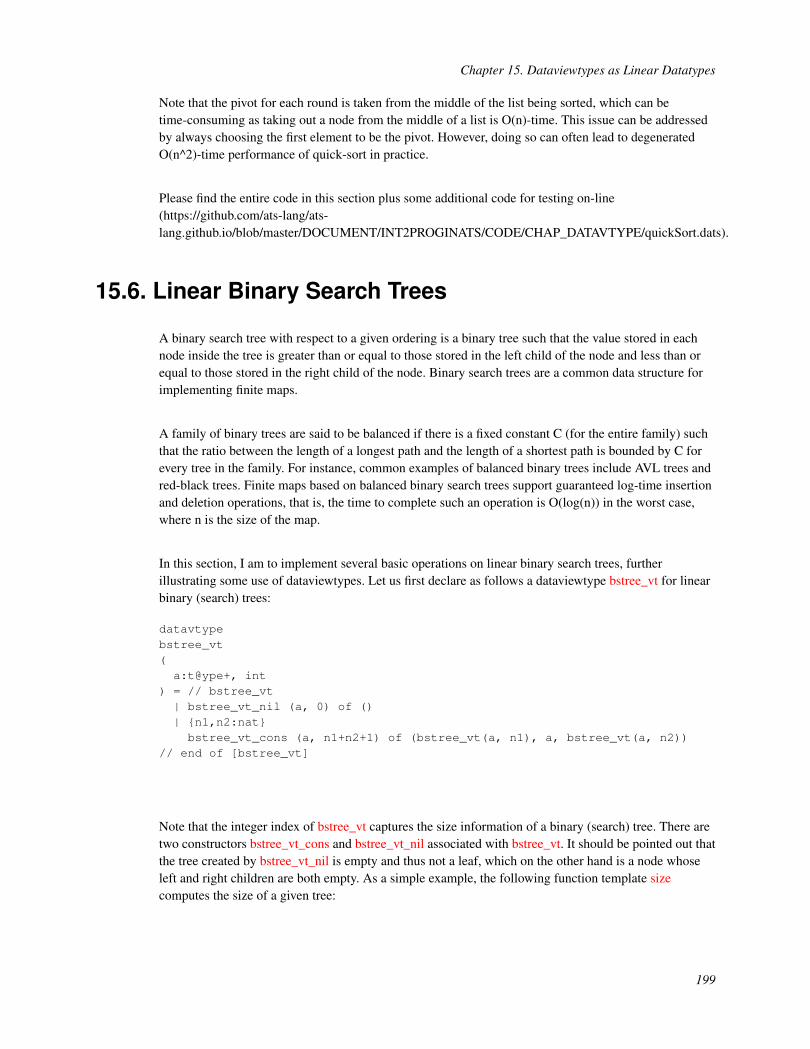
Chapter 15. Dataviewtypes as Linear Datatypes
Note that the pivot for each round is taken from the middle of the list being sorted, which can betime-consuming as taking out a node from the middle of a list is O(n)-time. This issue can be addressedby always choosing the first element to be the pivot. However, doing so can often lead to degeneratedO(n^2)-time performance of quick-sort in practice.
Please find the entire code in this section plus some additional code for testing on-line(https://github.com/ats-lang/ats-lang.github.io/blob/master/DOCUMENT/INT2PROGINATS/CODE/CHAP_DATAVTYPE/quickSort.dats).
15.6. Linear Binary Search Trees
A binary search tree with respect to a given ordering is a binary tree such that the value stored in eachnode inside the tree is greater than or equal to those stored in the left child of the node and less than orequal to those stored in the right child of the node. Binary search trees are a common data structure forimplementing finite maps.
A family of binary trees are said to be balanced if there is a fixed constant C (for the entire family) suchthat the ratio between the length of a longest path and the length of a shortest path is bounded by C forevery tree in the family. For instance, common examples of balanced binary trees include AVL trees andred-black trees. Finite maps based on balanced binary search trees support guaranteed log-time insertionand deletion operations, that is, the time to complete such an operation is O(log(n)) in the worst case,where n is the size of the map.
In this section, I am to implement several basic operations on linear binary search trees, furtherillustrating some use of dataviewtypes. Let us first declare as follows a dataviewtype bstree_vt for linearbinary (search) trees:
datavtypebstree_vt(a:t@ype+, int
) = // bstree_vt| bstree_vt_nil (a, 0) of ()| {n1,n2:nat}bstree_vt_cons (a, n1+n2+1) of (bstree_vt(a, n1), a, bstree_vt(a, n2))
// end of [bstree_vt]
Note that the integer index of bstree_vt captures the size information of a binary (search) tree. There aretwo constructors bstree_vt_cons and bstree_vt_nil associated with bstree_vt. It should be pointed out thatthe tree created by bstree_vt_nil is empty and thus not a leaf, which on the other hand is a node whoseleft and right children are both empty. As a simple example, the following function template sizecomputes the size of a given tree:
199

Chapter 15. Dataviewtypes as Linear Datatypes
fun{a:t@ype} size{n:nat} .<n>.(t: !bstree_vt (a, n)
) : int (n) =case+ t of| bstree_vt_nil () => 0| bstree_vt_cons
(tl, _, tr) => 1 + size (tl) + size (tr)// end of [size]
Assume that we have a binary search tree with repect to some ordering. If a predicate P on the elementsstored in the tree possesses the property that P(x1) implies P(x2) whenever x1 is less than x2 (accordingto the ordering), then we can locate the least element in the tree that satisfies the predicate P byemploying so-called binary search as is demonstrated in the following implementation of search:
fun{a:t@ype} search{n:nat} .<n>.
(t: !bstree_vt (a, n), P: (&a) -<cloref> bool
) : Option_vt (a) =case+ t of| @bstree_vt_cons
(tl, x, tr) =>if P (x) then letval res = search (tl, P)val res = (case+ res of| ~None_vt () => Some_vt (x) | _ => res
) : Option_vt (a)infold@ (t); res
end else letval res = search (tr, P) in fold@ (t); res
end // end of [if]| @bstree_vt_nil () => (fold@ (t); None_vt ())
// end of [search]
Clearly, if the argument t of search ranges over a family of balanced trees, then the time-complexity ofsearch is O(log(n)) (assuming that P is O(1)).
Let us next see some code implementing an operation that inserts a given element into a binary searchtree:
fun{a:t@ype
200

Chapter 15. Dataviewtypes as Linear Datatypes
} insert{n:nat} .<n>.(t: bstree_vt (a, n), x0: &a, cmp: cmp(a)
) : bstree_vt (a, n+1) =case+ t of| @bstree_vt_cons
(tl, x, tr) => letval sgn = compare<a> (x0, x, cmp)
inif sgn <= 0 then letval () = tl := insert (tl, x0, cmp)
infold@ (t); t
end else letval () = tr := insert (tr, x0, cmp)
infold@ (t); t
end (* end of [if] *)end // end of [bstree_vt_cons]
| ~bstree_vt_nil () =>bstree_vt_cons (bstree_vt_nil, x0, bstree_vt_nil)
// end of [bstree_vt_nil]// end of [insert]
When inserting an element, the function template insert extends the given tree with a new leaf nodecontaining the element, and this form of insertion is often referred to as leaf-insertion. There is anotherform of insertion often referred to as root-insertion, which always puts at the root position the new nodecontaining the inserted element. The following function template insertRT is implemented to perform astandard root-insertion operation:
fun{a:t@ype} insertRT{n:nat} .<n>.(t: bstree_vt (a, n), x0: &a, cmp: cmp(a)
) : bstree_vt (a, n+1) =case+ t of| @bstree_vt_cons
(tl, x, tr) => letval sgn = compare<a> (x0, x, cmp)
inif sgn <= 0 then letval tl_ = insertRT (tl, x0, cmp)val+@bstree_vt_cons (_, tll, tlr) = tl_val () = tl := tlrprval () = fold@ (t)val () = tlr := t
infold@ (tl_); tl_
end else let
201

Chapter 15. Dataviewtypes as Linear Datatypes
val tr_ = insertRT (tr, x0, cmp)val+@bstree_vt_cons (trl, _, trr) = tr_val () = tr := trlprval () = fold@ (t)val () = trl := t
infold@ (tr_); tr_
endend // end of [bstree_vt_cons]
| ~bstree_vt_nil () =>bstree_vt_cons (bstree_vt_nil, x0, bstree_vt_nil)
// end of [bstree_vt_nil]// end of [insertRT]
The code immediately following the first recursive call to insertRT performs a right tree rotation. Let ususe T(tl, x, tr) for a tree such that its root node contains the element x and its left and right children are tland tr, respectively. Then a right rotation turns T(T(tll, xl, tlr), x, tr) into T(tll, xl, T(tlr, x, tr)). The codeimmediately following the second recursive call to insertRT performs a left tree rotation, which turnsT(tl, x, T(trl, xr, trr)) into T(T(tl, x, tlr), xr, trr).
To further illustrate tree rotations, I present as follows two function templates lrotate and rrotate, whichimplement the left and right tree rotations, respectively:
fn{a:t@ype} lrotate{l,l_tl,l_x,l_tr:addr}{nl,nr:int | nl >= 0; nr > 0}
(pf_tl: bstree_vt (a, nl) @ l_tl
, pf_x: a @ l_x, pf_tr: bstree_vt (a, nr) @ l_tr| t: bstree_vt_cons_unfold (l, l_tl, l_x, l_tr), p_tl: ptr l_tl, p_tr: ptr l_tr) : bstree_vt (a, 1+nl+nr) = letval tr = !p_trval+@bstree_vt_cons (trl, _, trr) = trval () = !p_tr := trlprval () = fold@ (t); val () = trl := t
infold@ (tr); tr
end // end of [lrotate]
fn{a:t@ype} rrotate{l,l_tl,l_x,l_tr:addr}{nl,nr:int | nl > 0; nr >= 0}
(pf_tl: bstree_vt (a, nl) @ l_tl
, pf_x: a @ l_x
202

Chapter 15. Dataviewtypes as Linear Datatypes
, pf_tr: bstree_vt (a, nr) @ l_tr| t: bstree_vt_cons_unfold (l, l_tl, l_x, l_tr), p_tl: ptr l_tl, p_tr: ptr l_tr) : bstree_vt (a, 1+nl+nr) = letval tl = !p_tlval+@bstree_vt_cons (tll, x, tlr) = tlval () = !p_tl := tlrprval () = fold@ (t); val () = tlr := t
infold@ (tl); tl
end // end of [rrotate]
Given 4 addresses L0, L1, L2 and L3, the type bstree_vt_cons_unfold(L0, L1, L2, l3) is for a tree nodecreated by a call to bstree_vt_cons such that the node is located at L0 and the three arguments ofbstree_vt_cons are located at L1, L2 and L3, and the proofs for the at-views associated with L1, L2 andL3 are put in the store for currently available proofs.
The function template insertRT for root-insertion can now be implemented as follows by making directuse of lrotate and rrotate:
fun{a:t@ype} insertRT {n:nat} .<n>.(t: bstree_vt (a, n), x0: &a, cmp: cmp(a)
) : bstree_vt (a, n+1) =case+ t of| @bstree_vt_cons
(tl, x, tr) => letprval pf_x = view@xprval pf_tl = view@tlprval pf_tr = view@trval sgn = compare<a> (x0, x, cmp)
inif sgn <= 0 then letval () = tl := insertRT<a> (tl, x0, cmp)
inrrotate<a> (pf_tl, pf_x, pf_tr | t, addr@tl, addr@tr)
end else letval () = tr := insertRT<a> (tr, x0, cmp)
inlrotate<a> (pf_tl, pf_x, pf_tr | t, addr@tl, addr@tr)
end (* end of [if] *)end // end of [bstree_vt_cons]
| ~bstree_vt_nil () =>bstree_vt_cons (bstree_vt_nil, x0, bstree_vt_nil)
// end of [bstree_vt_nil]// end of [insertRT]
203

Chapter 15. Dataviewtypes as Linear Datatypes
I would like to point out that neither insert nor insertRT is tail-recursive. While it is straightforward togive the former a tail-recursive implementation, there is no direct way to do the same to the latter. Inorder to implement root-insertion in a tail-recursive manner, we are in need of binary search trees withparental pointers (so as to allow each node to gain direct access to its parent), which can be done withdataviews but not with dataviewtypes.
Please find the entire code in this section plus some additional code for testing on-line(https://github.com/ats-lang/ats-lang.github.io/blob/master/DOCUMENT/INT2PROGINATS/CODE/CHAP_DATAVTYPE/bstree_vt.dats).
15.7. Transition from Datatypes to Dataviewtypes
Many programmers are likely to find it a rather involved task to write code manipulating values ofdataviewtypes. When handling a complex data structure, I myself often try to first use a datatype tomodel the data structure and implement some functionalities of the data structure based the datatype. Ithen change the datatype into a corresponding dataviewtype and modify the implementation accordinglyto make it work with the dataviewtype. I now present as follows an implementation of linear red-blacktrees that is directly based on a previous implementation of functional red-black trees, illustratingconcretely a kind of gradual transition from datatypes to dataviewtypes that can greatly reduce the levelof difficulty one may otherwise encounter in an attempt to program with dataviewtypes directly.
The following declaration of dataviewtype rbtree is identical to the previous declaration of datatyperbtree except the keyword datavtype being now used instead of the keyword datatype:
#define BLK 0; #define RED 1sortdef clr = {c:int | 0 <= c; c <= 1}
datavtype rbtree(a: t@ype+, int(*c*), int(*bh*), int(*v*)
) = // element type, color, black height, violations| rbtree_nil (a, BLK, 0, 0) of ((*void*))| {c,cl,cr:clr}{bh:nat}{v:int}{c==BLK && v==0 || c == RED && v==cl+cr}rbtree_cons (a, c, bh+1-c, v) of (int c, rbtree0 (a, cl, bh), a, rbtree0 (a, cr, bh))
// end of [rbtree]
where rbtree0 (a:t@ype, c:int, bh:int) = rbtree (a, c, bh, 0)
At the first sight, the following function template insfix_l is greatly more involved that a previous versionof the same name (for manipulating functional red-black trees):
fn{a:t@ype
204
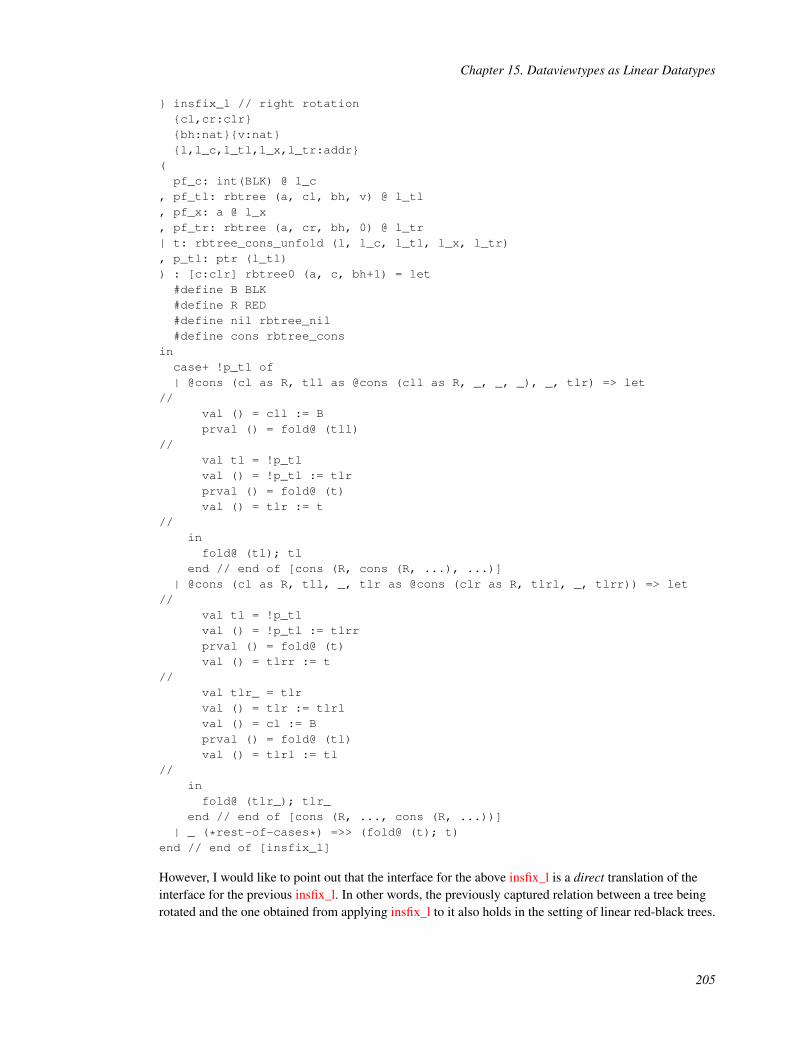
Chapter 15. Dataviewtypes as Linear Datatypes
} insfix_l // right rotation{cl,cr:clr}{bh:nat}{v:nat}{l,l_c,l_tl,l_x,l_tr:addr}
(pf_c: int(BLK) @ l_c
, pf_tl: rbtree (a, cl, bh, v) @ l_tl, pf_x: a @ l_x, pf_tr: rbtree (a, cr, bh, 0) @ l_tr| t: rbtree_cons_unfold (l, l_c, l_tl, l_x, l_tr), p_tl: ptr (l_tl)) : [c:clr] rbtree0 (a, c, bh+1) = let#define B BLK#define R RED#define nil rbtree_nil#define cons rbtree_cons
incase+ !p_tl of| @cons (cl as R, tll as @cons (cll as R, _, _, _), _, tlr) => let
//val () = cll := Bprval () = fold@ (tll)
//val tl = !p_tlval () = !p_tl := tlrprval () = fold@ (t)val () = tlr := t
//infold@ (tl); tl
end // end of [cons (R, cons (R, ...), ...)]| @cons (cl as R, tll, _, tlr as @cons (clr as R, tlrl, _, tlrr)) => let
//val tl = !p_tlval () = !p_tl := tlrrprval () = fold@ (t)val () = tlrr := t
//val tlr_ = tlrval () = tlr := tlrlval () = cl := Bprval () = fold@ (tl)val () = tlrl := tl
//infold@ (tlr_); tlr_
end // end of [cons (R, ..., cons (R, ...))]| _ (*rest-of-cases*) =>> (fold@ (t); t)
end // end of [insfix_l]
However, I would like to point out that the interface for the above insfix_l is a direct translation of theinterface for the previous insfix_l. In other words, the previously captured relation between a tree beingrotated and the one obtained from applying insfix_l to it also holds in the setting of linear red-black trees.
205
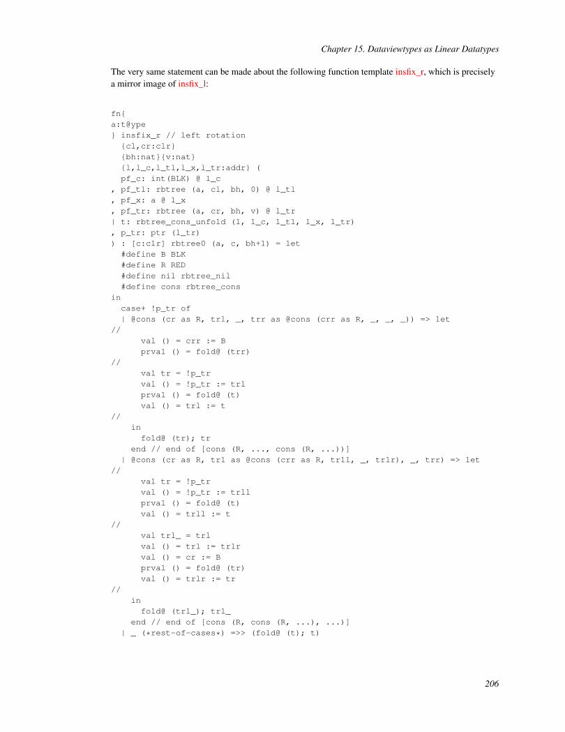
Chapter 15. Dataviewtypes as Linear Datatypes
The very same statement can be made about the following function template insfix_r, which is preciselya mirror image of insfix_l:
fn{a:t@ype} insfix_r // left rotation{cl,cr:clr}{bh:nat}{v:nat}{l,l_c,l_tl,l_x,l_tr:addr} (pf_c: int(BLK) @ l_c
, pf_tl: rbtree (a, cl, bh, 0) @ l_tl, pf_x: a @ l_x, pf_tr: rbtree (a, cr, bh, v) @ l_tr| t: rbtree_cons_unfold (l, l_c, l_tl, l_x, l_tr), p_tr: ptr (l_tr)) : [c:clr] rbtree0 (a, c, bh+1) = let#define B BLK#define R RED#define nil rbtree_nil#define cons rbtree_cons
incase+ !p_tr of| @cons (cr as R, trl, _, trr as @cons (crr as R, _, _, _)) => let
//val () = crr := Bprval () = fold@ (trr)
//val tr = !p_trval () = !p_tr := trlprval () = fold@ (t)val () = trl := t
//infold@ (tr); tr
end // end of [cons (R, ..., cons (R, ...))]| @cons (cr as R, trl as @cons (crr as R, trll, _, trlr), _, trr) => let
//val tr = !p_trval () = !p_tr := trllprval () = fold@ (t)val () = trll := t
//val trl_ = trlval () = trl := trlrval () = cr := Bprval () = fold@ (tr)val () = trlr := tr
//infold@ (trl_); trl_
end // end of [cons (R, cons (R, ...), ...)]| _ (*rest-of-cases*) =>> (fold@ (t); t)
206

Chapter 15. Dataviewtypes as Linear Datatypes
end // end of [insfix_r]
As can be expected, the following function template rbtree_insert is essentially a direct translation of theone of the same name for inserting an element into a functional red-black tree:
externfun{a:t@ype}rbtree_insert{c:clr}{bh:nat}
(t: rbtree0 (a, c, bh), x0: &a, cmp: cmp a
) : [bh1:nat] rbtree0 (a, BLK, bh1)
implement{a}rbtree_insert(t, x0, cmp) = let
//#define B BLK#define R RED#define nil rbtree_nil#define cons rbtree_cons//fun ins{c:clr}{bh:nat} .<bh,c>.
(t: rbtree0 (a, c, bh), x0: &a
) : [cl:clr; v:nat | v <= c] rbtree (a, cl, bh, v) =(case+ t of| @cons (
c, tl, x, tr) => letprval pf_c = view@cprval pf_tl = view@tlprval pf_x = view@xprval pf_tr = view@trval sgn = compare<a> (x0, x, cmp)
inif sgn < 0 then letval [cl:int,v:int] tl_ = ins (tl, x0)val () = tl := tl_
inif (c = B)then (insfix_l<a>(pf_c, pf_tl, pf_x, pf_tr | t, addr@tl)
// end of [insfix_l]) else letval () = c := R in fold@{a}{..}{..}{cl}(t); t
end // end of [if]
207

Chapter 15. Dataviewtypes as Linear Datatypes
end else if sgn > 0 then letval [cr:int,v:int] tr_ = ins (tr, x0)val () = tr := tr_
inif (c = B)then (insfix_r<a>(pf_c, pf_tl, pf_x, pf_tr | t, addr@tr)
// end of [insfix_r]) else letval () = c := R in fold@{a}{..}{..}{cr}(t); t
end // end of [if]end else (fold@{a}{..}{..}{0} (t); t)
end // end of [cons]| ~nil () => cons{a}{..}{..}{0}(R, nil, x0, nil)
) (* end of [ins] *)//val t = ins (t, x0)//in//case+ t of @cons(c as R, _, _, _) => (c := B; fold@ (t); t) | _ =>> t//end // end of [rbtree_insert]
I literally implemented the above rbtree_insert by making a copy of the previous implementation ofrbtree_insert for functional red-black trees and then properly modifying it to make it pass typechecking.Although this process of copying-and-modifying is difficult to be described formally, it is fairlystraightforward to follow in practice as it is almost entirely guided by the error messages issued duringtypechecking.
Please find the entire code in this section plus some additional code for testing on-line(https://github.com/ats-lang/ats-lang.github.io/blob/master/DOCUMENT/INT2PROGINATS/CODE/CHAP_DATAVTYPE/rbtree.dats).A challenging as well as rewarding exercise is for the reader to implement an operation that deletes anelement from a given linear red-black tree.
208

Chapter 16. Abstract Views and Viewtypes
I have so far given a presentation of views that solely focuses on at-views and the views built on top ofat-views. This is largely due to at-views being the form of most widely used views in practice and alsobeing the first form of views supported in ATS. However, other forms of views can be readily introducedinto ATS abstractly. Even in a case where a view can be defined based on at-views (or other forms ofviews), one may still want to introduce it as an abstract view (accompanied with certain proof functionsfor performing view-changes). Often what the programmer really needs is to figure out conceptuallywhether abstractly defined views and proof functions for manipulating them actually make sense. This isa bit like arguing whether a function is computable: There is rarely a need, if at all, to actually encode thefunction as a Turing-machine to prove its being computable. IMHO, learning proper use of abstractviews and abstract viewtypes is a necessary step for one to take in order to employ linear typeseffectively in practice to deal with resource-related programming issues.
16.1. Simple Linear Objects
Objects in the physical world are conspicuously linear: They cannot be created from nothing or simplygo vanished by turning into nothing. Thus, it is only natural to assign linear types to values that representphysical objects. I choose the name simple linear object here to refer to a linear value representing anobject of some sort that does not contain built-in mechanism for supporting inheritance.
Let us now take a look at a concrete example of simple linear object. The following code presents aninterface for a timer (that is, stopwatch):
//absvtype timer_vtypevtypedef timer = timer_vtype//fun timer_new (): timerfun timer_free (x: timer): voidfun timer_start (x: !timer): voidfun timer_finish (x: !timer): voidfun timer_pause (x: !timer): voidfun timer_resume (x: !timer): voidfun timer_get_ntick (x: !timer): uintfun timer_reset (x: !timer): void//
The state of a timer is given the record type timer_struct defined as follows:
//typedeftimer_struct = @{started= bool // the timer has started
, running= bool // the timer is running
209

Chapter 16. Abstract Views and Viewtypes
// the tick number recorded when the timer, ntick_beg= uint // was turned on last time, ntick_acc= uint // the number of accumulated ticks} (* end of [timer_struct] *)//
The following linear datatype timer is declared for timers, and the abstract type timer_vtype is assumedto equal timer:
//datavtype timer =TIMER of (timer_struct)
//assume timer_vtype = timer//
Various functions on timers can now be readily implemented. Let us first see the code for creating andfreeing timers:
implementtimer_new () = let//val timer = TIMER (_)val TIMER (x) = timer//val () = x.started := falseval () = x.running := falseval () = x.ntick_beg := 0uval () = x.ntick_acc := 0u//prval () = fold@ (timer)//intimer
end // end of [timer_new]
implementtimer_free (timer) =let val ~TIMER _ = timer in (*nothing*) end
// end of [timer_free]
The function for starting a timer can be implemented as follows:
implementtimer_start(timer) = letval+@TIMER(x) = timer
210

Chapter 16. Abstract Views and Viewtypes
val () = x.started := trueval () = x.running := trueval () = x.ntick_beg := the_current_tick_get ()val () = x.ntick_acc := 0uprval () = fold@ (timer)
in// nothing
end // end of [timer_start]
where the_current_tick_get is a function for reading the current time (represented as a number of ticks):
extern fun the_current_tick_get (): uint
A timer can be stopped or paused. The function for stopping a timer can be implemented as follows:
implementtimer_finish(timer) = letval+@TIMER(x) = timerval () = x.started := falseval () =if x.running then{val () = x.running := falseval () = x.ntick_acc :=x.ntick_acc + the_current_tick_get () - x.ntick_beg
} (* end of [val] *)prval () = fold@ (timer)
in// nothing
end // end of [timer_finish]
A timer can be paused and then resumed. The following code implements the functions for pausing andresuming a timer:
implementtimer_pause(timer) = letval+@TIMER(x) = timerval () =if x.running then{val () = x.running := falseval () = x.ntick_acc :=x.ntick_acc + the_current_tick_get () - x.ntick_beg
} (* end of [val] *)prval () = fold@ (timer)
211

Chapter 16. Abstract Views and Viewtypes
in// nothing
end // end of [timer_pause]
implementtimer_resume(timer) = letval+@TIMER(x) = timerval () =if x.started && ~(x.running) then{val () = x.running := trueval () = x.ntick_beg := the_current_tick_get ()
} (* end of [if] *) // end of [val]prval () = fold@ (timer)
in// nothing
end // end of [timer_resume]
As can be expected, the amount of time between the point where a timer is paused and the point wherethe timer is resumed is not counted.
It is also possible to reset a timer by calling the function timer_reset:
implementtimer_reset(timer) = letval+@TIMER(x) = timerval () = x.started := falseval () = x.running := falseval () = x.ntick_beg := 0uval () = x.ntick_acc := 0uprval () = fold@ (timer)
in// nothing
end // end of [timer_reset]
In order to read the time accumulated by a timer, the function timer_get_ntick can be called:
implementtimer_get_ntick(timer) = letval+@TIMER(x) = timervar ntick: uint = x.ntick_accval () =if x.running then (ntick := ntick + the_current_tick_get () - x.ntick_beg
) (* end of [if] *) // end of [val]prval () = fold@ (timer)
212

Chapter 16. Abstract Views and Viewtypes
inntick
end // end of [timer_get_ntick]
A straightforward approach to implementing the_current_tick_get can be based directly on the functionclock_gettime:
local
staload "libc/SATS/time.sats"
in (* in-of-local *)
implementthe_current_tick_get () = letvar tv: timespec // uninitializedval err = clock_gettime (CLOCK_REALTIME, tv)val ((*void*)) = assertloc (err >= 0)prval ((*void*)) = opt_unsome{timespec}(tv)
in$UNSAFE.cast2uint(tv.tv_sec)
end // end of [the_current_tick_get]
end // end of [local]
Note that the library flag -lrt may be needed in order to have link-time access to clock_gettime as thefunction is in librt.
Please find on-line (https://github.com/ats-lang/ats-lang.github.io/blob/master/DOCUMENT/INT2PROGINATS/CODE/CHAP_ABSVTYPE/timer.dats) theentirety of the code presented in this section plus some testing code.
16.2. Memory Allocation and Deallocation
The issue of memory allocation and deallocation is of paramount importance in systems programming,where garabage collection (GC) at run-time may not even be allowed. Handling memory managementsafely and efficiently is a long standing problem of great challenge in programming, and its novelsolution in ATS is firmly rooted in the paradigm of programming with theorem-proving (PwTP).
The following function malloc_gc is available in ATS for memory allocation:
fun malloc_gc{n:nat}(n: size_t n): [l:agz] (b0ytes n @ l, mfree_gc_v (l) | ptr l)
// end of [malloc_gc]
213

Chapter 16. Abstract Views and Viewtypes
The sort agz is a subset sort defined for addresses that are not null:
sortdef agz = {a:addr | a > null} // [gz] for great-than-zero
Given an integer N, the type b0ytes(N) is a shorthand for @[byte?][N], which is for an array of Nuninitialized bytes. Therefore, the at-view b0ytes(N)@L is the same as the array-view array_v(byte?, L,N), where L is a memory location. The view constructor mfree_gc_v is abstract. For a given location L,the view mfree_gc_v(L) stands for a form of capability that allows allocated memory at location L to befreed (or reclaimed) by the following function mfree_gc:
fun mfree_gc{l:addr}{n:nat}(pfat: b0ytes(n) @ l, pfgc: mfree_gc_v (l) | p: ptr l): void
// end of [free_gc]
Note that mfree_gc_v(L) is so far the first form of view we have encountered that is not built on top ofany at-views.
In practice, it is rather cumbersome to deal with bytes directly. The function ptr_alloc is available forallocating memory to store a single value (of certain type) and the function ptr_free for deallocating suchmemory:
fun{a:vt0p}ptr_alloc ():<> [l:agz] (a? @ l, mfree_gc_v (l) | ptr l)
// end of [ptr_alloc]
fun ptr_free{a:t@ype}{l:addr}(pfgc: mfree_gc_v (l), pfat: a @ l | p: ptr l):<> void = "mac#%"
// end of [ptr_free]
In addition, the function array_ptr_alloc is for allocating memory to store an array of values (of certaintype), and the function array_ptr_free is for deallocating such memory:
fun{a:vt0p}array_ptr_alloc{n:int}
(asz: size_t n
) : [l:agz](array_v (a?, l, n), mfree_gc_v (l) | ptr l
) // end of [array_ptr_alloc]
fun{}array_ptr_free{a:vt0p}{l:addr}{n:int}
(
214

Chapter 16. Abstract Views and Viewtypes
array_v (a?, l, n), mfree_gc_v (l) | ptr l) : void // end of [array_ptr_free]
I now give a realistic and interesting example involving both array allocation and deallocation. Thefollowing two functions templates msort1 and msort2 perform merge-sort on a given array:
typedef cmp (a:t@ype) = (&a, &a) -> int
externfun{a:t@ype} msort1 {n:nat}(A: &(@[a][n]), n: size_t n, B: &(@[a?][n]), cmp: cmp(a)): void
// end of [msort1]
externfun{a:t@ype} msort2 {n:nat}(A: &(@[a][n]), n: size_t n, B: &(@[a?][n]) >> @[a][n], cmp: cmp(a)): void
// end of [msort2]
It is well-known that merging two sorted segments of a given array requires additional space. Whenmsort1 is called on arrays A and B, the array A is the one to be sorted and the array B is some kind ofscratch area needed to perform merging (of sorted array segments). When a call to msort1 returns, thesorted version of A is still sotred in A. What msort2 does is similar but the sorted version of A is storedin B when a call to msort2 returns. As a good exercise, I suggest that the interested reader take the effortto give a mutually recursive implementation of msort1 and msort2. An implementation of merge-sortbased on msort1 can be readily given as follows:
externfun{a:t@ype} mergeSort{n:nat}(A: &(@[a][n]), n: size_t n, cmp: cmp(a)): void
// end of [mergeSort]
implement{a}(*tmp*)mergeSort(A, n, cmp) = letval (pfat, pfgc | p) = array_ptr_alloc<a> (n)val ((*void*)) = msort1 (A, n, !p, cmp)val ((*void*)) = array_ptr_free (pfat, pfgc | p)
in// nothing
end // end of [mergeSort]
215

Chapter 16. Abstract Views and Viewtypes
Clearly, an array is first allocated (to be used as a scratch area) and then deallocated after it is no longerneeded.
It is also allowed for a function to allocate memory on its call-stack by calling a special function alloca,which is given the following type in ATS:
(*staload "libc/SATS/alloa.sats"
*)fun alloca{dummy:addr}{n:int} (pf: void@dummy | n: size_t (n)
) : [l:addr] (bytes(n) @ l, bytes(n) @ l -> void@dummy | ptr(l))
The type assigned to alloca makes it extremely unlikely for someone to unintentionally write well-typedcode in ATS that may erroneourly attempt to access memory obtained from calling alloca after thecalling function has returned.
The following function array_ptr_alloca_tsz is the same as alloca dynamically but it is given a type thatis often more convenient to use:
funarray_ptr_alloca_tsz{a:vt0p}{dummy:addr}{n:int}
(pf: void@dummy | asz: size_t(n), tsz: sizeof_t(a)
) : [l:addr] (array(a?,n)@l, array(a?,n)@l -> void@dummy | ptr(l))
As an example, the function template mergeSort implemented above can also be implemented asfollows:
implement{a}(*tmp*)mergeSort(A, n, cmp) = letval tsz = sizeof<a>var dummy: void = ()prval pf = view@dummyval (pfat, fpfat | p
) = array_ptr_alloca_tsz{a}(pf | n, tsz)val ((*void*)) = msort1<a> (A, n, !p, cmp)prval ((*void*)) = view@dummy := fpfat (pfat)
in// nothing
end // end of [mergeSort]
where the array used as a scratch area during merge-sort is allocated on the call-stack of mergeSort.While this implementation of mergeSort may seem interesting, it is actually inferior to the previousimplementation as calling alloca to allocate a large chunk of memory can readily lead to a crash for
216

Chapter 16. Abstract Views and Viewtypes
which the cause is often very difficult to determine. In general, choosing alloca over malloc is difficult tojustify, and any call to the former should be scrutinized.
The entire implementation of merge-sort on arrays plus some testing code is available on-line(https://github.com/ats-lang/ats-lang.github.io/blob/master/DOCUMENT/INT2PROGINATS/CODE/CHAP_ABSVTYPE/mergeSort.dats).
16.3. Example: Array-Based Circular Buffers
Array-based circular buffers are of common use in practice. For instance, in a typical client/server model,a circular buffer can be employed to hold requests issued by multiple clients that are then processed bythe server according to the first-in-first-out (FIFO) policy. In a case where each request needs to be givena priority (chosen from a fixed set), a circular buffer can be created for each priority to hold requests ofthat particular priority.
Let us declare a linear abstract type (that is, abstract viewtype) as follows for values representing circularbuffers:
absvtypecbufObj (a:vt@ype+, m:int, n: int) = ptr
Such values are considered simple linear objects (as inheritance is not an issue to be dealt with in thissetting). Given a viewtype VT and two integers M and N, the viewtype cbufObj(VT, M, N) is for a givenbuffer of maximal capacity M that currently holds N elements of the type VT.
Some properties on the parameters of cbufObj can be captured by introducing the following prooffunction:
//prfunlemma_cbufObj_param{a:vt0p}{m,n:int}(buf: !cbufObj(a, m, n)): [m>=n; n>=0] void
//
The interface for the following two function templates indicates that they can be called to compute thecapacity and current size of a buffer:
//fun{a:vt0p}cbufObj_get_cap{m,n:int} (buf: !cbufObj(a, m, n)): size_t(m)
//fun{a:vt0p}cbufObj_get_size{m,n:int}(buf: !cbufObj(a, m, n)): size_t(n)
217

Chapter 16. Abstract Views and Viewtypes
//
While it is straightforward to use cbufObj_get_cap and cbufObj_get_size to tell whether a buffer iscurrently empty or full, a direct approach is likely to be more efficient. The following two functiontemplates check for the emptiness and fullness of a given circular buffer:
//fun{a:vt0p}cbufObj_is_empty{m,n:int}(buf: !cbufObj(a, m, n)): bool(n==0)
//fun{a:vt0p}cbufObj_is_full{m,n:int}(buf: !cbufObj(a, m, n)): bool(m==n)
//
The functions for creating and destroying circular buffers are named cbufObj_new and cbufObj_free,respectively:
//fun{a:vt0p}cbufObj_new{m:pos}(m: size_t(m)): cbufObj(a, m, 0)
//fun cbufObj_free{a:vt0p}{m:int}(buf: cbufObj(a, m, 0)): void
//
Note that a buffer can be freed only if it contains no elements as an element (of some viewtype) maycontain resources. If elements in a buffer are of some (non-linear) type, then the following function canbe called to clear out all the elements stored in the buffer:
funcbufObj_clear{a:t@ype}{m,n:int}(buf: !cbufObj(a, m, n) >> cbufObj(a, m, 0)): void
// end of [cbufObj_clear]
The next two functions are for inserting/removing an element into/from a given buffer, which areprobably the most frequently used operations on buffers:
//fun{a:vt0p}
218

Chapter 16. Abstract Views and Viewtypes
cbufObj_insert{m,n:int | n < m}
(buf: !cbufObj(a, m, n) >> cbufObj(a, m, n+1), x: a
) : void // end of [cbufObj_insert]//fun{a:vt0p}cbufObj_remove{m,n:int | n > 0}(buf: !cbufObj(a, m, n) >> cbufObj(a, m, n-1)): (a)
//
Please find on-line the file circbuf.sats (https://github.com/ats-lang/ats-lang.github.io/blob/master/DOCUMENT/INT2PROGINATS/CODE/CHAP_ABSVTYPE/circbuf.sats)containing the entirety of the interface for functions creating, destroying and manipulating circularbuffers.
There are many simple and practical ways to implement the abstract type cbufObj and the functionsdeclared in circbuf.sats (https://github.com/ats-lang/ats-lang.github.io/blob/master/DOCUMENT/INT2PROGINATS/CODE/CHAP_ABSVTYPE/circbuf.sats).In the file circbuf.dats (https://github.com/ats-lang/ats-lang.github.io/blob/master/DOCUMENT/INT2PROGINATS/CODE/CHAP_ABSVTYPE/circbuf.dats),I give an implementation that employs four pointers p_beg, p_end, p_frst and p_last to represent acircular buffer: p_beg and p_end are the starting and finishing addresses of the underline array,respectively, and p_frst and p_last are the starting addresses of the occupied and unoccupied segments (inthe array), respectively. What is special about this implementation is its employing a style ofprogramming that deliberately eschews the need for proof construction. While code written in this styleis not guaranteed to be type-safe, the style can nonetheless be of great practical value in a setting whereconstructing formal proofs is deemed too costly a requirement to be fully fulfilled. Anyone who tries togive a type-safe implementation for the functions declared in circbuf.sats (https://github.com/ats-lang/ats-lang.github.io/blob/master/DOCUMENT/INT2PROGINATS/CODE/CHAP_ABSVTYPE/circbuf.sats)should likely find some genuine appreciation for this point.
In the file circbuf2.dats (https://github.com/ats-lang/ats-lang.github.io/blob/master/DOCUMENT/INT2PROGINATS/CODE/CHAP_ABSVTYPE/circbuf2.dats),I give another implementation in which a circular buffer is represented as a pointer p_beg plus threeintegers m, n and f: p_beg points to the starting location of the underline array, m is the size of the array(that is, the capacity of the buffer), n is the number of elements currently stored in the buffer and f is thetotal number of elements that have so far been removed from the buffer. Again, proof construction isdelibrately eschewed in this implementation.
219
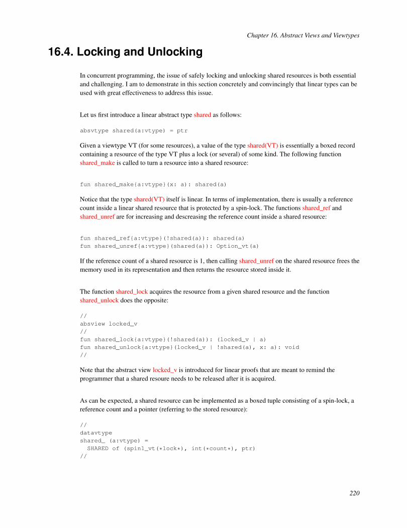
Chapter 16. Abstract Views and Viewtypes
16.4. Locking and Unlocking
In concurrent programming, the issue of safely locking and unlocking shared resources is both essentialand challenging. I am to demonstrate in this section concretely and convincingly that linear types can beused with great effectiveness to address this issue.
Let us first introduce a linear abstract type shared as follows:
absvtype shared(a:vtype) = ptr
Given a viewtype VT (for some resources), a value of the type shared(VT) is essentially a boxed recordcontaining a resource of the type VT plus a lock (or several) of some kind. The following functionshared_make is called to turn a resource into a shared resource:
fun shared_make{a:vtype}(x: a): shared(a)
Notice that the type shared(VT) itself is linear. In terms of implementation, there is usually a referencecount inside a linear shared resource that is protected by a spin-lock. The functions shared_ref andshared_unref are for increasing and descreasing the reference count inside a shared resource:
fun shared_ref{a:vtype}(!shared(a)): shared(a)fun shared_unref{a:vtype}(shared(a)): Option_vt(a)
If the reference count of a shared resource is 1, then calling shared_unref on the shared resource frees thememory used in its representation and then returns the resource stored inside it.
The function shared_lock acquires the resource from a given shared resource and the functionshared_unlock does the opposite:
//absview locked_v//fun shared_lock{a:vtype}(!shared(a)): (locked_v | a)fun shared_unlock{a:vtype}(locked_v | !shared(a), x: a): void//
Note that the abstract view locked_v is introduced for linear proofs that are meant to remind theprogrammer that a shared resoure needs to be released after it is acquired.
As can be expected, a shared resource can be implemented as a boxed tuple consisting of a spin-lock, areference count and a pointer (referring to the stored resource):
//datavtypeshared_ (a:vtype) =SHARED of (spin1_vt(*lock*), int(*count*), ptr)
//
220

Chapter 16. Abstract Views and Viewtypes
assume shared = shared_//
Note that the type spin1_vt is for linear spin-locks. The function shared_ref is implemented as follows:
implementshared_ref{a}(sh) = let
//val+@SHARED(spin, count, _) = sh
//valspin = // for temp. useunsafe_spin_vt2t(spin)
//val(pf | ()) = spin_lock(spin)val c0 = countval () = count := c0 + 1val ((*void*)) = spin_unlock(pf | spin)prval ((*void*)) = fold@sh//in$UN.castvwtp1{shared(a)}(sh)
end // end of [shared_ref]
Clearly, the implementation makes use of several unsafe casts. An implementation without such castswould be highly involved even if it could be done. The spin-lock must be acquired before the bindingbetween c0 and the integer stored in count is formed for otherwise a race condition can appear. Thefunction shared_unref is implemented as follows:
implementshared_unref{a}(sh) = let
//val+@SHARED(spin, count, _) = sh
//valspin = // for temp. useunsafe_spin_vt2t(spin)
//val(pf | ()) = spin_lock(spin)val c0 = countval () = count := c0 - 1val ((*void*)) = spin_unlock(pf | spin)prval ((*void*)) = fold@sh//in
221

Chapter 16. Abstract Views and Viewtypes
//ifc0 <= 1then letval+~SHARED(spin, _, x) = shval ((*freed*)) = spin_vt_destroy(spin)
inSome_vt($UN.castvwtp0{a}(x))
end // end of [then]else letprval () = $UN.cast2void(sh) in None_vt()
end // end of [else]//end // end of [shared_unref]
In the case where the reference count is 1, then the shared resource is freed, the spin-lock in it isdestroyed, and the resource in it is returned.
The functions shared_lock and shared_unlock are implemented as follows:
implementshared_lock{a}(sh) = let
//val+@SHARED(spin, _, x) = sh//valspin =unsafe_spin_vt2t(spin)
//val(pf | ()) = spin_lock(spin)//val x0 = $UN.castvwtp0{a}(x)//prval () = fold@sh//in($UN.castview0(pf) | x0)
end // end of [shared_lock]
implementshared_unlock{a}(pf | sh, x0) = let
//val+@SHARED(spin, _, x) = sh//valspin =unsafe_spin_vt2t(spin)
//
222

Chapter 16. Abstract Views and Viewtypes
val () = x := $UN.castvwtp0{ptr}(x0)//val () =spin_unlock($UN.castview0(pf) | spin)
//prval () = fold@sh//in// nothing
end // end of [shared_unlock]
In the case of shared_lock, please notice that the content stored in the variable x is read out after thespin-lock is acquired. This is crucial for otherwise a race condition can readily appear. In the case ofshared_unlock, the content of the variable x is updated before the acquired spin-lock is released.
Please find on-line the file shared_vt.dats (https://github.com/ats-lang/ats-lang.github.io/blob/master/DOCUMENT/INT2PROGINATS/CODE/CHAP_ABSVTYPE/shared_vt.dats)containing the entirety of the code presented in this section. In addition, the file also contains animplementation of three threads that move in locked steps: thread 0 moves; thread 1 moves; thread 2moves; thread 0 moves; thread 1 moves; thread 2 moves; etc.
16.5. Linear Channels for Asynchronous IPC
In this section, I will present an implementation of linear channels to support asynchronouscommunication between threads. This is also a very fitting occasion for me to advocate what I often referto as programmer-centric program verification.
A communication channel between threads is essentially a queue wrapped in some kind of protectionmechanism needed for guarding against race conditions. Assume that a queue is of a fixed capacity, thatis, the capacity of the queue is fixed after its creation. If the queue is full, then inserting an element into itresults in a failure. If the queue is empty, then removing an element from it results in a failure. In order toprevent inserting into a full queue or removing from an empty queue, I could first introduce a linearabstract type for queues as follows:
absvtypequeue_vtype(a:vt@ype+, int(*m*), int(*n*))vtypedef queue(a:vt@ype,m:int,n:int) = queue_vtype(a,m,n)
where the type queue(VT,M,N) is for a queue of capacity M that currently contains N elements of typeVT. Then the functions for inserting into and removing from a queue are expected to be given thefollowing interface:
//fun{a:vt0p}queue_insert{m,n:nat | m > n}
223

Chapter 16. Abstract Views and Viewtypes
(!queue(a, m, n) >> queue(a, m, n+1), a): void//fun{a:vt0p}queue_remove{m,n:nat | n > 0}(!queue(a, m, n) >> queue(a, m, n-1)): (a)
//
The presented abstract type queue can indeed work very well for the task of implementing linearchannels. However, I will not continue with this version of queue further for I intend to present a style ofprogram verification that is less rigorous but far more flexible.
Following is another version of abstract type queue:
//absvtypequeue_vtype(a:vt@ype+, int(*id*)) = ptr//vtypedefqueue(a:vt0p, id:int) = queue_vtype(a, id)vtypedef queue(a:vt0p) = [id:int] queue(a, id)//
Given a viewtype VT and an integer ID, queue(VT,ID) is for a queue containing elements of the type VTthat can be uniquely identified with the integer ID. So one may think of ID as some form of stamp. Thefollowing declared function queue_isnil is for testing whether a given queue is empty:
//absprop ISNIL(id:int, b:bool)//fun{a:vt0p}queue_isnil{id:int}(!queue(a, id)): [b:bool] (ISNIL(id, b) | bool(b))//
Given an integer ID, a proof of the prop ISNIL(ID,true) (ISNIL(ID,false)) means that the queue uniquelyidentified by ID is (not) empty. Similarly, the following declared function queue_isful is for testingwhether a given queue is full:
//absprop ISFUL(id:int, b:bool)//fun{a:vt0p}queue_isful{id:int}(!queue(a, id)): [b:bool] (ISFUL(id, b) | bool(b))//
Given an integer ID, a proof of the prop ISFUL(ID,true) (ISFUL(ID,false)) means that the queueuniquely identified by ID is (not) full.
224

Chapter 16. Abstract Views and Viewtypes
The functions queue_insert and queue_remove for inserting into and removing from a given queue cannow be given the following interface:
//externfun{a:vt0p}queue_insert{id:int}
(ISFUL(id, false)
| xs: !queue(a, id) >> queue(a, id2), x: a) : #[id2:int] void//externfun{a:vt0p}queue_remove{id:int}
(ISNIL(id, false) | xs: !queue(a, id) >> queue(a, id2)
) : #[id2:int] a // end-of-fun//
Note that either inserting an element into a queue or removing an element from a queue assigns a newstamp to the queue. This is essential for interpreting ISNIL and ISFUL in the manner presented above.
In order to call queue_insert on a given queue, one needs to have a proof attesting to the queue being notfull. Such a proof is obtained if calling queue_isful on the queue returns false. Similarly, in order to callqueue_remove on a given queue, one can first call queue_isnil on the queue to obtain a proof attesting tothe queue being not empty.
What is really of concern here is not to actually verify that queue_isnil and queue_isful have the interfaceassigned to them. Instead, the focus is on ensuring that queue_insert is never applied to a full queue andqueue_remove is never applied to an empty queue under the assumption that queue_isnil and queue_isfulhave the assigned interface. I refer to this form of program verification as being programmer-centricbecause its correctness is not formally established in an objective manner. I myself find thatprogrammer-centric program verification is very flexible and effective in practice. If we believe thatconstructing informal mathematical proofs can help one check whether the proven statements are valid,then it is only natural to believe that programmer-centric program verification can also help one checkwhether verified programs are correct.
Let us now start to implement linear channels for asynchronous communication between threads. First,let us declare a linear abstract type channel as follows:
absvtype channel_vtype(a:vt@ype+) = ptrvtypedef channel(a:vt0p) = channel_vtype(a)
The function for inserting an element into a channel is given the following interface:
225

Chapter 16. Abstract Views and Viewtypes
fun{a:vt0p} channel_insert (!channel(a), a): void
The caller of channel_insert is blocked if the channel is full. Similarly, the function for removing anelement from a channel is given the following interface:
fun{a:vt0p} channel_remove (chan: !channel(a)): (a)
The caller of channel_remove is blocked if the channel is empty.
Let a channel be represented as follows:
//datavtypechannel_ ={l0,l1,l2,l3:agz} CHANNEL of@{cap=intGt(0)
, spin=spin_vt(l0), rfcnt=intGt(0), mutex=mutex_vt(l1), CVisnil=condvar_vt(l2), CVisful=condvar_vt(l3), queue=ptr // deqarray} (* end of [channel] *)//assume channel_vtype(a:vt0p) = channel_//
There are 7 fields in the record representing a channel; the cap field stores an integer indicating the(fixed) capacity of the channel; the spin field stores a spin-lock for protecting the reference count in thefield of the name rfcnt; the mutex field stores a mutex for protecting the queue in the field of the namequeue; the field CVisnil stores a conditional variable for the situation where a caller (holding the mutex)wants to wait for the condition that the queue becomes not empty; the field CVisful stores a conditionalvariable for the situation where a caller (holding the mutex) wants to wait for the condition that the queuebecomes not full.
The function channel_insert is given the following implementation:
implement{a}(*tmp*)channel_insert(chan, x0) = let
//val+CHANNEL{l0,l1,l2,l3}(ch) = chan
val mutex = unsafe_mutex_vt2t(ch.mutex)val (pfmut | ()) = mutex_lock (mutex)val xs =
226

Chapter 16. Abstract Views and Viewtypes
$UN.castvwtp0{queue(a)}((pfmut | ch.queue))val ((*void*)) = channel_insert2<a> (chan, xs, x0)prval pfmut = $UN.castview0{locked_v(l1)}(xs)val ((*void*)) = mutex_unlock (pfmut | mutex)//in// nothing
end // end of [channel_insert]
where the auxiliary function channel_insert2 is given the following interface:
fun{a:vt0p}channel_insert2(!channel(a), !queue(a) >> _, a): void
Please note that channel_insert2 is called when the caller is holding the mutex inside the channel.Following is an implementation for channel_insert2:
implement{a}(*tmp*)channel_insert2(chan, xs, x0) = let
//val+CHANNEL{l0,l1,l2,l3}(ch) = chan
//val (pf | isful) = queue_isful (xs)//in//ifisfulthen letprval(pfmut, fpf) =__assert () where{externpraxi __assert (): vtakeout0(locked_v(l1))
}val mutex = unsafe_mutex_vt2t(ch.mutex)val CVisful = unsafe_condvar_vt2t(ch.CVisful)val ((*void*)) = condvar_wait (pfmut | CVisful, mutex)prval ((*void*)) = fpf (pfmut)
inchannel_insert2 (chan, xs, x0)
end // end of [then]else letval isnil = queue_isnil (xs)val ((*void*)) = queue_insert (pf | xs, x0)val ((*void*)) =if isnil.1
227

Chapter 16. Abstract Views and Viewtypes
then condvar_broadcast(unsafe_condvar_vt2t(ch.CVisnil))// end of [if]
in// nothing
end // end of [else]//end // end of [channel_insert2]
The logic behind channel_insert2 can be explained as follows. If the queue in the given channel is full,the caller calls condvar_wait to release the mutex it holds and then wait on the conditional variable storedin the field CVisful of the channel; after the caller regains the mutex after being awoken by a signal sentto the conditioanl variable, it calls channel_insert2 recursively. If the queue in the given channel is notfull, then the caller insert a given element into the queue stored in the field queue and then returns. Notethat channel_insert2 is a tail-recursive function that essentially corresponds to a standard while-loopoften appearing in C code for handling the wait on a conditional variable.
By following the above implementation for channel_insert (and channel_insert2), it should be prettystraightforward for one to figure out an implementation for channel_remove. I leave it as an exercise.
Please find on-line the file channel_vt.dats (https://github.com/ats-lang/ats-lang.github.io/blob/master/DOCUMENT/INT2PROGINATS/CODE/CHAP_ABSVTYPE/channel_vt.dats)containing the entirety of the code presented in this section plus some code for testing.
228

V. Programming with FunctionTemplates

Chapter 17. From Genericity to Late-Binding
The support for function templates in ATS is deeply ingrained in the design and implementation of ATS.Primarily, function templates are meant to provide a general approach to code reuse in ATS that is highlyflexible (in terms of applicability) while incurring minimal run-time overhead if any. Both ATSPRE (thatis, ATSLIB/prelude) and ATSLIB/libats are nearly entirely template-based, and the templates in theselibraries are for use by atsopt to generate C code that implements template instances in the ATS sourcebeing compiled. The library files of ATS for linking (libatslib.a and libatslib.so) are minimal,and they are not even necessary for compiling ATS source into executable binaries.
The code employed for illustration in this chapter plus some additional code for testing is availableon-line (https://github.com/ats-lang/ats-lang.github.io/blob/master/DOCUMENT/INT2PROGINATS/CODE/CHAP_FNTMPINT/).
17.1. Genericity of Template Implementations
As is briefly explained in Part I of the book, function templates can be seen as a natural solution to theproblem of supporting parametric polymorphism in the presence of native unboxed data. However,function templates can do much more than just supporting parametric polymorphism. Let myprint be afunction template of the following interface:
fun{a:t@ype} myprint (x: a): void
Given a value, myprint is supposed to print out some kind of representation for this value. For example,we can implement myprint as follows:
implement{a} myprint (x) = print_string "?"
This implementation of myprint is often referred to as a (fully) generic template implementation due tono restriction being imposed on the template parameter. Following is another way to code the sameimplementation:
implement(a) myprint<a> (x) = print_string "?"
Clearly, the above generic implementation of myprint is unsatisfactory as it outputs no specificinformation on a given value. We may want to implement myprint as follows for only values of the typeint:
implement myprint<int> (x) = print_int (x)
where print_int is called to print out a given integer. This implementation of myprint is often referred toas a specific template implementation due to the template parameter being bound to a specific type (that
230

Chapter 17. From Genericity to Late-Binding
is, int in this case). The following code implements myprint for list-values (that is, values of type List(T)for some type T):
implement(a)myprint<List(a)> (xs) =case+ xs of| list_nil () => ()| list_cons (x, xs) =>
(myprint<a> (x); myprint<List(a)> (xs))
This implementation of myprint is often referred to as a partially generic template implementation. Inorder for an instance of myprint to use this implementation, the template parameter for the instance mustbe of the form List(T) for some type T. As an example, the following code calls an instance of myprint toprint out a list of two integer lists:
(*** The output is "0123401234"
*)val ys = $list{int}(0,1,2,3,4)val yss = $list{List(int)}(ys, ys)val ((*void*)) = myprint<List(List(int))> (yss)val ((*void*)) = print_newline((*void*))
Implementations of a function template can be ordered according to an obvious partial ordering referredto as genericity ordering: The genericity of one implementation is less than or equal to that of anotherone if the former implementation is an instance of the latter one. Please note that the first-fit (instead ofbest-fit) strategy is employed to locate the template implementation needed for compiling a giventemplate instance. More specifically, locating the template implementation for a particular templateinstance follows the standard principle of lexical scoping to search for the first one that is available foruse.
In practice, there is quite a bit of subtlety in locating a template implementation for a template instance.Let myprint2 be a function template of the following interface:
fun{a:t@ype} myprint2 (x: a): int
Following is a partially generic implementation of myprint2:
//implement(a)myprint2<List(a)> (xs) =case+ xs of| list_nil () => ()| list_cons (x, xs) =>
(myprint<a> (x); 1 + myprint2 (xs))//
231

Chapter 17. From Genericity to Late-Binding
This template implementation actually behaves very differently from what one might have expected.Note that the template parameter of the called instance of myprint2 in the body of the implementation issynthesized to be a type of the form list(a, N) for some static term N (of the sort int). As this form cannever match List(T) for any type T, the called instance of the template myprint2 cannot be compiledaccording to the given template implementation of myprint2. This issue can be readily fixed by passingexplicity the type List(a) (as a template parameter) to the called instance of myprint2:
//implement(a)myprint2<List(a)> (xs) =case+ xs of| list_nil () => ()| list_cons (x, xs) =>
(myprint<a> (x); 1 + myprint2<List(a)> (xs))//
The instance myprint2<List(a)> in this example is often referred to as a recursive instance. In general, itis a good programming practice to avoid using recursive instances. For example, the followingequivalent implementation of myprint2 makes no use of recursive instances:
//implement(a)myprint2<List(a)>(xs) = let
//funaux(xs: List(a)): int =//case+ xs of| list_nil () => 0| list_cons (x, xs) => (myprint<a>(x); 1 + aux(xs))//inaux (xs)
end // end of [myprint2<List(a)>]//
Please find on-line the file myprint.dats (https://github.com/ats-lang/ats-lang.github.io/blob/master/DOCUMENT/INT2PROGINATS/CODE/CHAP_FNTMPINT/myprint.dats)containing the entirety of the code presented in this section plus some testing code.
232

Chapter 17. From Genericity to Late-Binding
17.2. Example: Generic Operations on Numbers
There are many types of numbers in ATS. With function templates, we can greatly enhance code sharingin numerical computation. For example, we can give a generic implementation of matrix multiplicationof the following interface:
fun{a:t@ype}matrix_mul{p,q,r:int}
(p: int(p)
, q: int(q), r: int(r), A: &matrix(a, p, q), B: &matrix(a, q, r), C: &matrix(a?, p, r) >> matrix(a, p, r)) : void // end of [matrix_mul]
and then use it to immediately obtain implementations of matrix multiplication for matrices of integers,matrices of floating point numbers, matrices of floating point complex numbers, etc. This approach isclearly far superior to relying on error-prone macros in C.
Let us take a look at a concrete example involving generic operations on numbers. The following codegives a standard implementation of the factorial function:
//externfun fact(n: int): int//implementfact(n) =if n > 0 then n * fact(n-1) else 1
// end of [fact]//
When applied to 100, fact is likely to return 0. This can be easily understood as the true value of thefactorial of 100 is a multiple of 232 and the multiplication operation on integers of the type int is probablymodulo 232. Suppose that we want to replace this multiplication operation with the one on floating pointnumbers of double precision. This can be done by implementing a slight variant of fact as follows
//externfun factd(n: int): double//implementfactd(n) =if n > 0 then n * factd(n-1) else 1.0
// end of [factd]
233

Chapter 17. From Genericity to Late-Binding
//
When applied to 100, factd should return a large floating point number. Obviously, there is a great deal ofcode duplication between the implementations of fact and factd. We can readily eliminate thisduplication by introducing a generic implementation of the factorial function as follows:
//externfun{a:t@ype} gfact(n: int): a//implement{a}(*tmp*)gfact(n) = (//if n > 0then gmul_int_val<a>(n, gfact<a>(n-1))else gnumber_int<a>(1)//) (* end of [gfact] *)//
With a bit of help from the support for overloading in ATS, we can rewrite gfact as follows:
implement{a}(*tmp*)gfact(n) = let//overload * with gmul_int_val//in//if n > 0then n * gfact<a>(n-1) else gnumber_int<a>(1)//end (* end of [gfact] *)
We can now implement fact and factd as follows:
//implement fact(n) = gfact<int>(n)implement factd(n) = gfact<double>(n)//
There is support in ATS based on the GNU multiple precision arithmetic library (GMPLIB) for integersof unlimited precision. The following code presents a way to compute the true value of the factorial of100:
//staload _(*T*) ="{$LIBATSHWXI}/intinf/DATS/intinf_t.dats"
234
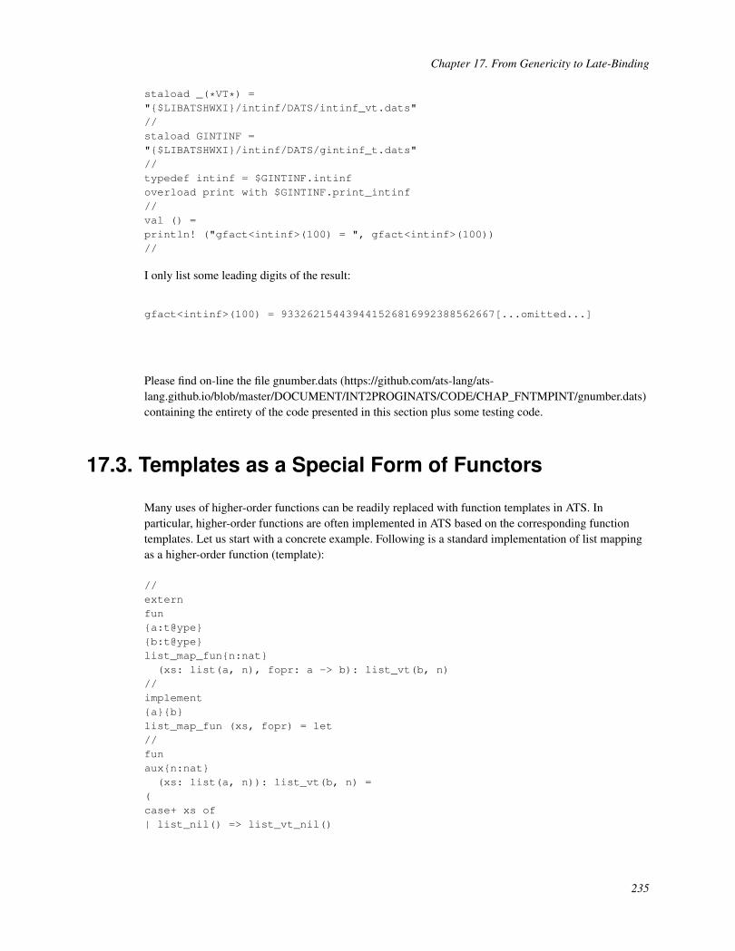
Chapter 17. From Genericity to Late-Binding
staload _(*VT*) ="{$LIBATSHWXI}/intinf/DATS/intinf_vt.dats"//staload GINTINF ="{$LIBATSHWXI}/intinf/DATS/gintinf_t.dats"//typedef intinf = $GINTINF.intinfoverload print with $GINTINF.print_intinf//val () =println! ("gfact<intinf>(100) = ", gfact<intinf>(100))//
I only list some leading digits of the result:
gfact<intinf>(100) = 933262154439441526816992388562667[...omitted...]
Please find on-line the file gnumber.dats (https://github.com/ats-lang/ats-lang.github.io/blob/master/DOCUMENT/INT2PROGINATS/CODE/CHAP_FNTMPINT/gnumber.dats)containing the entirety of the code presented in this section plus some testing code.
17.3. Templates as a Special Form of Functors
Many uses of higher-order functions can be readily replaced with function templates in ATS. Inparticular, higher-order functions are often implemented in ATS based on the corresponding functiontemplates. Let us start with a concrete example. Following is a standard implementation of list mappingas a higher-order function (template):
//externfun{a:t@ype}{b:t@ype}list_map_fun{n:nat}(xs: list(a, n), fopr: a -> b): list_vt(b, n)
//implement{a}{b}list_map_fun (xs, fopr) = let//funaux{n:nat}(xs: list(a, n)): list_vt(b, n) =
(case+ xs of| list_nil() => list_vt_nil()
235

Chapter 17. From Genericity to Late-Binding
| list_cons(x, xs) => list_vt_cons(fopr(x), aux(xs)))//inaux(xs)
end // end of [list_map_fun]//
Given a list of cerntain length and a function (which is envless), list_map_fun returns a linear list of thesame length. Unfortunately, list_map_fun cannot be called on a list and a closure-function. We certainlycan implement a variant of list_map_fun of the following interface by essentially duplicating theimplementation of list_map_fun:
//externfun{a:t@ype}{b:t@ype}list_map_cloref{n:nat}(xs: list(a, n), fopr: a -<cloref1> b): list_vt(b, n)
//
While list_map_cloref can be called on a list and a closure-function, the closure-function that is formedat run-time to be passed to a call to list_map_cloref most likely becomes garbage immediately after thecall returns. Without garbage collection (GC), the memory for storing the closure is leaked. We surelyhave many good reasons for avoiding using a higher-order function like list_map_cloref when doingembedded programming in ATS.
A proper way to implement list mapping (as I see it) is given as follows:
//externfun{a:t@ype}{b:t@ype}list_map{n:nat}(xs: list(a, n)): list_vt(b, n)
//externfun{a:t@ype}{b:t@ype} list_map$fopr(x: a): b//implement{a}{b}list_map (xs) = let//funaux{n:nat}(xs: list(a, n)): list_vt(b, n) =
(case+ xs of
236

Chapter 17. From Genericity to Late-Binding
| list_nil() => list_vt_nil()| list_cons(x, xs) => list_vt_cons(list_map$fopr<a><b>(x), aux(xs))) (* end of [aux] *)//inaux(xs)
end // end of [list_map]//
The function template list_map is given in a style that is often referred to as being functorial: list_mapcan be thought of as a functor in Standard ML that applies to a module consisting of a single functionlist_map$fopr. In SML, each argument of a functor, which itself is a module, needs to be constructed andthen passed to the functor explcitly. In ATS, the template implementation needed for compiling aparticular template instance is located through a search procedure (that follows the standard principle oflexical scoping).
With list_map, we can implement list_map_fun as follows in a straightforward manner:
implement{a}{b}list_map_fun(xs, fopr) = let//implement list_map$fopr<a><b> (x) = fopr(x)//inlist_map<a><b> (xs)
end // end of [list_map_fun]
Please note that list_map$fopr being implemented inside the body of list_map_fun allows theimplementation to gain direct access to the argument fopr of list_map_fun. It is in this sense thattemplates in ATS are often referred to as embeddable templates as they can be directly implemented inthe bodies of functions. We can implement list_map_cloref similarly as follows:
implement{a}{b}list_map_cloref(xs, fopr) = let//implement list_map$fopr<a><b> (x) = fopr(x)//inlist_map<a><b> (xs)
end // end of [list_map_cloref]
For those who are familiar with functors in SML, the implementation of list_map_fun andlist_map_cloref should clearly remind them of functor application.
Please find on-line the file list_map.dats (https://github.com/ats-lang/ats-lang.github.io/blob/master/DOCUMENT/INT2PROGINATS/CODE/CHAP_FNTMPINT/list_map.dats)containing the entirety of the code presented in this section plus some testing code.
237

Chapter 17. From Genericity to Late-Binding
17.4. Example: Templates for Loop Construction
Beginners in functional programming (FP) who have already acquired some knowledge of imperativeprogramming often ask about ways to construct for-loops and while-loops in FP. A commonly givenanswer is that loop constructs are unnecessary in FP as they can be readily replaced with higher-orderfunctions. Let us first see some thorny issues with this answer.
The following code in C implements a function that returns the sum of the first n natural numbers whenapplied to a natural number n:
inttally (int n) {int i, res;for (i = 0, res = 0; i < n; i += 1) res += i;return res;
}
This function tally can be given the following equivalent implementation in ATS:
funtally(n: int
) : int = loop (0, 0) where{fun loop (i: int, res: int): int =if i < n then loop (i + 1, res + i) else res
}
where the tail-recursive function loop is just a translation of the for-loop in C.
When someone claims that loop constructs can be replaced with higher-order functions, he or sheprobably means to construct loops with a function like the following one:
funfor_loop(count: int, limit: int, fwork: (int) -<cloref1> void
) : void = (//if count < limitthen (fwork(count); for_loop(count+1, limit, fwork)) else ()
// end of [if]) (* end of [for_loop] *)
For example, the following function tally2 is directly based on for_loop:
fun
238

Chapter 17. From Genericity to Late-Binding
tally2(n: int
) : int = letval res = ref<int> (0)
infor_loop (0, n, lam (i) => !res := !res + i); !res
end // end of [tally2]
While both tally and tally2 return the same result when applied to a given natural number, they behavevery differently at run-time. In particular, each call to tally2 creates a (persistent) reference on heap fortemporary use; the reference becomes garbage immediately after the call returns. Compared to tally,tally2 is inefficient both time-wise and memory-wise.
To eliminate the need for reference creation in tally2, we turn for_loop into the following functiontemplate for_loop2:
//fun{env:t@ype} for_loop2(count: int, limit: int
, env: &env >> _, fwork: (int, &env >> _) -<cloref1> void) : void = (//ifcount < limitthen (fwork(count, env); for_loop2<env> (count+1, limit, env, fwork)
) else ()// end of [if]//) (* end of [for_loop2] *)
We can further turn tally2 into the following tally3 based on for_loop2:
funtally3(n: int
) : int = letvar res: int = 0
infor_loop2<int> (0, n, res, lam (i, res) => res := res + i); res
end // end of [tally3]
While tally3 improves upon tally2, it is still a bit unsatisfactory. Clearly, the closure function formedbefore tally3 calls for_loop2 becomes garbage immediately after the call returns. It is plausible to expectthat an optimizing C compiler (e.g., gcc and clang) can eliminate the need for actual closure formation
239

Chapter 17. From Genericity to Late-Binding
when it compiles the C code generated from ATS source, but there is no guarantee. In order to have sucha guarantee, we can evolve for_loop2 into the following function template for_loop3:
fun{env:t@ype} for_loop3(count: int, limit: int, env: &env >> _
) : void = (//ifcount < limitthen (for_loop3$fwork<env>(count, env); for_loop3<env>(count+1, limit, env)
) else ()// end of [if]//) (* end of [for_loop3] *)
where for_loop3$fwork is given the interface below:
fun{env:t@ype} for_loop3$fwork(count: int, env: &env >> _): void
Finally, we can turn tally3 into tally4 as follows:
funtally4(n: int
) : int = let//var res: int = 0//implementfor_loop3$fwork<int> (i, res) = res := res + i//infor_loop3<int> (0, n, res); res
end // end of [tally4]
By inspecting the C code generated by atsopt from compiling tally4, we can see that the C code isessentially equivalent to the implementation of tally in C (given at the beginning of this section).
By now, the reader probably agrees with me if I say the statement should at least be considered grosslyinaccurate that claims loop constructs in FP can be readily replaced with higher-order functions. Please
240

Chapter 17. From Genericity to Late-Binding
find on-line the file loopcons.dats (https://github.com/ats-lang/ats-lang.github.io/blob/master/DOCUMENT/INT2PROGINATS/CODE/CHAP_FNTMPINT/loopcons.dats)containing the entirety of the code presented in this section plus some testing code.
17.5. Template-Based Support for Late-Binding
When asked about the meaning of object-oriented programming (OOP), Alan Kay once said that OOP tohim meant only messaging, local retention and protection and hiding of state-process, and extremelate-binding of all things.
In ATS, function templates can provide a highly flexible approach to supporting late-binding (of functioncalls). Let us first take a look at a simple example to see why late-binding can be so desirable. Thefollowing code declares a datatype intfloat such that each value of this declared type represents either aninteger or a floating point number (of double precision):
//datatypeintfloat = INT of int | FLOAT of double//
In order to print values of the type intfloat, we can implement print_intfloat as follows:
//funprint_intfloat(x: intfloat): void =
(case+ x of| INT(int) => print_int(int)| FLOAT(float) => print_double(float))//
where print_int and print_double are monomorphic functions for printing an integer and a floating pointnumber (of double precision), respectively. There are certainly many different ways to print integers andfloating point numbers, but print_intfloat only uses a particular one for integers (via print_int) and aparticular one for floating point numbers (via print_double). One possibility of avoiding this form ofextreme inflexibility is to define a higher-order function fprint_intfloat as follows:
//funfprint_intfloat(x: intfloat
, print_int: int -> void, print_double: double -> void) : void =
241

Chapter 17. From Genericity to Late-Binding
(case+ x of| INT(int) => print_int(int)| FLOAT(float) => print_double(float))//
With fprint_intfloat, one can decide to choose implementations for print_int and print_double at a laterstage. In this regard, I say that higher-order functions can support a form of late-binding. However, usinghigher-order functions in such a manner is not without serious problems. Basically, any function thatcalls print_int either directly or indirectly needs to be turned into a higher-order function, and the sameapplies to functions calling print_double as well. This style of programming with extensive use ofhigher-order functions can soon become extremely unwieldy when the number of functions grows largethat need to be treated like print_int and print_double.
Instead of using higher-order functions, we can rely on template functions to support late-binding (offunction calls). For example, the following code implements a template function tprint_intfloat forprinting values of the type intfloat:
//externfun{}tprint_int(int): voidexternfun{}tprint_double(double): voidexternfun{}tprint_intfloat(intfloat): void//(* ****** ****** *)//implementtprint_int<> (x) = print_int(x)implementtprint_double<> (x) = print_double(x)//(* ****** ****** *)//implementtprint_intfloat<> (x) =(case+ x of| INT(int) => tprint_int<> (int)| FLOAT(float) => tprint_double<> (float))//
Please note that the default implementations for tprint_int and tprint_double are based on print_int andprint_double, respectively. As can be expected, the following code outputs two lines:
242

Chapter 17. From Genericity to Late-Binding
//val () = (tprint_intfloat<> (INT(0)); print_newline()
) (* end of [val] *)//val () = (tprint_intfloat<> (FLOAT(1.0)); print_newline()
) (* end of [val] *)//
where the first line consists of the string "0" and the second one the string "1.000000". The followingcode also outputs two lines:
local//implementtprint_int<> (x) = print! ("INT(", x, ")")implementtprint_double<> (x) = print! ("FLOAT(", x, ")")//in (* in-of-local *)//val () = (tprint_intfloat<> (INT(0)); print_newline()
) (* end of [val] *)//val () = (tprint_intfloat<> (FLOAT(1.0)); print_newline()
) (* end of [val] *)//end // end of [local]
where the first line consists of the string "INT(0)" and the second one the string "FLOAT(1.000000)"). Inthe latter case, the calls to template instances tprint_int<> and tprint_double<> are compiled accordingto the implementations for tprint_int and tprint_double given between the keywords local and in.
Please find on-line the file intfloat.dats (https://github.com/ats-lang/ats-lang.github.io/blob/master/DOCUMENT/INT2PROGINATS/CODE/CHAP_FNTMPINT/intfloat.dats)containing the entirety of the code presented in this section plus some testing code.
243


