Introduction to Programming in R Introduction to the Rlanguage CCCB course on R and Bioconductor, May 2012,

Aedin Culhane aedin@jimmy.harvard.edu

May 16, 2012

I Obtaining and managing R

R can be downloaded from the website: http://cran.r-project.org/. See additional noteswhich give a very detailed description on downloading and installing R (and Bioconductor).

R is available for all platforms: Unix/Linux, Windows and Mac. In this course, we will concentrate onthe Windows implementation. The differences between the platforms are minor, so most of the materialis applicable to the other platforms.

See the associated file on the course website, in which I give detailed instructions on downloading andinstalling R and Bioconductor (for windows).

II The default R interface

This is the default user interface with the standard installation of R. In the course we will mostly useRStudio which provides a richer interface. RStudio can be obtained from www.rstudio.org)

• Start up R (go to the program Menu and find it in the Statistics folder)

• First, notice the different menus and icons in R. On the menu bar, there are the menus:

– File - load script, load/save session (workspace) or command history. Change Directory– Edit - Cut/Paste. GUI preferences

– View

– Misc - stop computations, list/remove objects in session

– Packages - allows one to install new, update packages

– Windows

– Help - An essential resource!

1

• The icons below will allow one to

– open script (.R file),

– load image (previous R session, .RData file)

– save .R script

– copy and paste

– stop a computation (this can be an important button, but the ESC also works!)

– print.

II.1 Default R Editor

• Within R, one can open an editor using the menu command File -> New script

• Can type commands in the editor

• Highlight the commands and type Ctrl^R to submit the commands for R evaluation

• Evaluation of the commands can be stopped by pressing the Esc key or the Stop button

• Saving (Ctrl^S) and opening saved commands (Ctrl^O)

• Can open a new editor by typing Ctrl^N

II.2 Setting R default properties (on Windows)

The first thing to do when starting an R session, is to ensure that you will be able to find your data andalso that your output will be saved to a useful location on your computer hard-drive. Therefore, checkthe "working directory".

This maybe set by default to the depths of the operating system (C:/program files/R), which is a poor"working" location. You may wish to change the default start location by right mouse clicking on theR icon on the desktop/start menu and changing the "Start In" property. For example make a folder’C:/work’, and make this as a "Start in" folder. Alternatively you can change your working directory,once you start R (see below)

III Starting out - Changing directory

The first thing to do when starting an R session, is to ensure that you will be able to find your data andalso that your output will be saved to a useful location on your computer hard-drive.

To change the default start location, right mouse click on the R icon on the (Windows) desktop/startmenu and changing the "Start In" property. For example make a folder ’C:/work’, and make this as a"Start in" folder. Alternatively you can change your working directory

2

When you start R, and see the prompt > , it may appear as if nothing is happening. This prompt is nowawaiting commands from you. This can be daunting to the new user, however it is easy to learn a fewcommands and get started.

First, to change the directory after you have started R. Use the file menu, to change directory: File ->Change dir If you wish to type R commands to set or change working directories, use the following

> getwd()

To change the directory:

setwd("C:/work")getwd()

I may create a new working directory for each R session which I call projectNameDate (eg colonJan13).

# check if the directory or file exisitsfile.exists("colonJan13")

# Create a directoryfolder

dir.create("colonJan13")

If you have files in the working directory, you can see the contents of your working folder using thefunctions/commands

> dir()> dir(pattern=".txt")

Within R Studio you can change and view the contents of a directory using the lower right panel. Clickon the Files tab. To set a direct a working directory, navigate to the directory you wish to set as yourhome directory. To navigate up a directory, click on the triple dot icon on the top right. Once you arein the correct directory and see your data files, click on the More (blue cogwheel), and select "Set asWorking Directory "

IV R Packages

By default, R is packaged with a small number of essential packages, however as we saw there aremany contributed R packages.

3

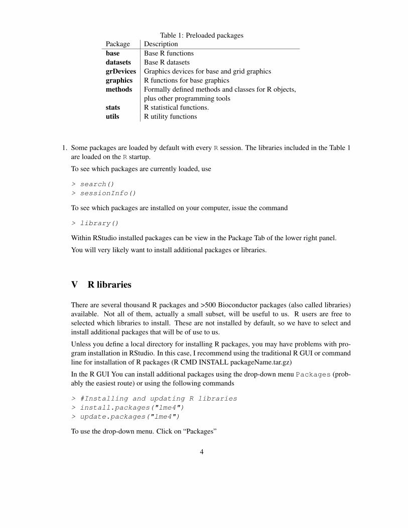
Table 1: Preloaded packagesPackage Descriptionbase Base R functionsdatasets Base R datasetsgrDevices Graphics devices for base and grid graphicsgraphics R functions for base graphicsmethods Formally defined methods and classes for R objects,

plus other programming toolsstats R statistical functions.utils R utility functions

1. Some packages are loaded by default with every R session. The libraries included in the Table 1are loaded on the R startup.

To see which packages are currently loaded, use

> search()> sessionInfo()

To see which packages are installed on your computer, issue the command

> library()

Within RStudio installed packages can be view in the Package Tab of the lower right panel.

You will very likely want to install additional packages or libraries.

V R libraries

There are several thousand R packages and >500 Bioconductor packages (also called libraries)available. Not all of them, actually a small subset, will be useful to us. R users are free toselected which libraries to install. These are not installed by default, so we have to select andinstall additional packages that will be of use to us.

Unless you define a local directory for installing R packages, you may have problems with pro-gram installation in RStudio. In this case, I recommend using the traditional R GUI or commandline for installation of R packages (R CMD INSTALL packageName.tar.gz)

In the R GUI You can install additional packages using the drop-down menu Packages (prob-ably the easiest route) or using the following commands

> #Installing and updating R libraries> install.packages("lme4")> update.packages("lme4")

To use the drop-down menu. Click on “Packages”

4

• Go to “Set CRAN mirror” and choose an available mirror (choose one close by, it’ll befaster hopefully).

• If you know the name of the package you want to install, or if you want to install all theavailable packages, click on “Packages” again and choose “Install package(s) from CRAN”To select more than one page, use shift-mouse click or control-mouse click.

• Installation of all packages takes some time and space on your computer.• If the name of the package is not known, you could use taskviews help or archives of the

mailing list to pinpoint one. Also look on the R website Task views description of packages(see Additional Notes in Installation which I have provided).

Once you have installed a package, you do NOT need to re-install it. But to load the library inyour current R session use the commands

> library(lme4) # Load a package> ## Or the alternative> require(lme4)> sessionInfo() #List all packages loaded in the current R session> library() # List all installed packages> data() # List all available example datasets

You can unload the loaded package pkg by

> detach(package:lme4)> search()

To get an information on a package, type

> library(help=lme4)

NOTE: Packages are often inter-dependent, and loading one may cause others to be automaticallyloaded.

VI Datasets in R

Both the R core installation and contributed R package contain datasets, which are useful example datawhen learning R. To list all available data sets:

> data()

To load a dataset, for example, the dataset women which gives the average heights and weights for 15American women aged 3039.

> data(women)> ls()> ls(pattern="w")

5

VII Getting help with functions and features

There are many resources for help in R.

• Emmanuel Paradis has an excellent beginners guide to R available from http://cran.r-project.org/doc/contrib/Paradis-rdebuts_en.pdf

• There is an introduction to R classes and objects on the R website http://cran.r-project.org/doc/manuals/R-intro.html and also see Tom Guirkes manual at http://manuals.bioinformatics.ucr.edu/home/R_BioCondManual

• Tom Short’s provides a useful short R reference card at http://cran.r-project.org/doc/contrib/Short-refcard.pdf

Within R, you can find help on any command (or find commands) using the follow:

• If you know the command (or part of it)

help(lm)?matrixapropos("mean")example(rep)

The last command will run all the examples included with the help for a particular function. Ifwe want to run particular examples, we can highlight the commands in the help window andsubmit them by typing Ctrl^V

• If you don’t know the command and want to do a keyword search for it.

> help.search("combination")> help.start()

help.search will open a html web browser or a MSWindows help browser (depending onthe your preferences) in which you can browse and search R documentation.

• Finally, there is a large R community who are incredibly helpful. There is a mailing list for R,Bioconductor and almost every R project. It is useful to search the archives of these mailing lists.Frequently you will find someone encountered the same problem as you, and previously askedthe R mailing list for help (and got a solution!).

• There are useful tools and resources on the web including:

– The R search engine http://www.Rseek.org

– R bloggers website http://www.r-bloggers.com/

6

VIII Interactive use of the R Editor

Note on the command line, the default prompt starts with an ’>’ If the command is not complete onone line, the continuation prompt is ’+’

Type q() to quit the program

VIII.1 R as a big calculator

Type the following into an R session (or copy and paste from this document).

> 2+2

[1] 4

> 2*2

[1] 4

> 2*100/4

[1] 50

> 2*100/4+2

[1] 52

> 2*100/(4+2)

[1] 33.33333

> 2^10

[1] 1024

> log(2)

7

[1] 0.6931472

> tmpVal<-log(2)> tmpVal

[1] 0.6931472

> exp(tmpVal)

[1] 2

> rnorm(5)

[1] -0.42284718 0.02583733 -0.78730662 -0.06056189[5] -1.46630342

Note you can recover previous commands using the up and down arrow keys. Indeed you can recoverthe previous expressions entered (default 25) into the R session using the function history.

rnorm generates 10 random numbers from a normal distribution. Type this a few times (hint: the uparrow key is useful).

Note even in the simple use of R as a calculator, it is useful to store intermediate results, (tmpVal=log(2)).In this case, we assigned a symbolic variable tmpVal. Note when you assign a value to such a vari-able, there is no immediate visible result. We need to print(tmpVal) or just type tmpVal in orderto see what value was assigned to tmpVal

IX Basic operators

IX.1 Comparison operators

• equal: ==

• not equal: !=

• greater/less than: > <

• greater/less than or equal: >= <=

> 1 == 1

[1] TRUE

8

IX.2 Logical operators

• AND & Returns TRUE if both comparisons return TRUE.

> x <- 1:10; y <- 10:1> x > y & x > 5

[1] FALSE FALSE FALSE FALSE FALSE TRUE TRUE TRUE TRUE[10] TRUE

• OR | Returns TRUE where at least one comparison returns TRUE.

> x == y | x != y

[1] TRUE TRUE TRUE TRUE TRUE TRUE TRUE TRUE TRUE TRUE

• NOT ! The ’!’ sign returns the negation (opposite) of a logical vector.

> !x > y

[1] TRUE TRUE TRUE TRUE TRUE FALSE FALSE FALSE FALSE[10] FALSE

X A few important points on R

• R is case sensitive, i.e. myData and Mydata are different names

• Elementary commands: expressions are evaluated, printed and value lost; assignments evaluateexpressions, passes value to a variable, but not automatically printed

> 2*5^2

[1] 50

> x <- 2*5^2> print(x)

[1] 50

• Assignment operators are: ’<-’, ’=’, ’->’

> 2*5^2

[1] 50

9

> y <- 2*5^2> z<-2*5^2> 2*5^2 -> z> print(y)

[1] 50

> x==y

[1] TRUE

> y==z

[1] TRUE

• ’<-’ is the most popular assignment operator, and ’=’ is a recent addition.

There is no space between < and −It is ’<-’ (less than and a minus symbol)

Although, unlikely, you may also see old code using ’_’, these is NOT used any more in R.

When assigning a value spaces are ignored so ’z<-3’ is equivalent to ’z <- 3’

• Arguments (parameters) to a function calls f(x), PROC are enclosed in round brackets. Even ifno arguments are passed to a function, the round brackets are required.

print(x)getwd()

• Comments can be put anywhere. To comment text, insert a hashmark #. Everything following itto end of the line is commented out (ignored, not evaluated).

print(y) # Here is a comment

• Note on brackets. It is very important to use the correct brackets.

Bracket Use() To set priorities 3*(2+4). Function calls f(x)[] Indexing in vectors, matrices, data frames{} Creating new functions. Grouping commands {mean(x); var(x)}

[[]] Indexing of lists

• ’==’ and ’=’ have very different uses in R. == is a binary operator, which test for equality (A==Bdetermines if A ’is equal to’ B ).

• Quotes, you can use both " double or ’ single quotes, as long as they are matched.

10

• For names, normally all alphanumeric symbols are allowed plus ’.’ and ’_’ Start names witha character [Aa-Zz] not a numeric character [0-9]. Avoid using single characters or functionnames t, c, q, diff, mean

• Commands can be grouped together with braces (’{’ and ’}’).

• Missing values called represented by NA

11

XI R Objects

• Everything (variable, functions etc) in R is an object

• Every object has a class

XI.1 Managing R Objects

R creates and manipulates objects: variables, matrices, strings, functions, etc. objects are stored byname during an R session.

During a R session, you may create many objects, if you wish to list the objects you have created in thecurrent session use the command

> objects()> ls()

The collection of objects is called workspace.

If you wish to delete (remove) objects, issue the commands:

rm(x,y,z, junk)ls()

where x, y, junk were the objects created during the session.

Note rm(list=ls()) will remove everything. Use with caution

XI.2 Types of R objects

Objects can be thought of as a container which holds data or a function. The most basic form of datais a single element, such as a single numeric or a character string. However one can’t do statistics onsingle numbers! Therefore there are many other objects in R.

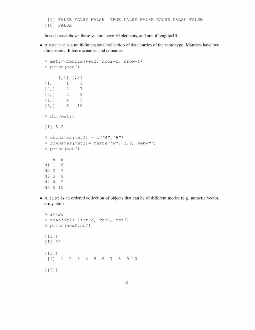
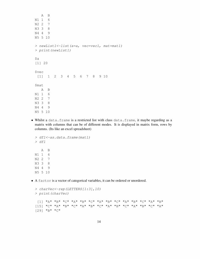
• A vector is an ordered collection of numerical, character, complex or logical objects. Vectorsare collection of atomic (same data type) components or modes. For example

> vec1<-1:10> vec2<-LETTERS[1:10]> vec3<-vec2=="D"> vec3

12

[1] FALSE FALSE FALSE TRUE FALSE FALSE FALSE FALSE FALSE[10] FALSE

In each case above, these vectors have 10 elements, and are of length=10.

• A matrix is a multidimensional collection of data entries of the same type. Matrices have twodimensions. It has rownames and colnames.

> mat1<-matrix(vec1, ncol=2, nrow=5)> print(mat1)

[,1] [,2][1,] 1 6[2,] 2 7[3,] 3 8[4,] 4 9[5,] 5 10

> dim(mat1)

[1] 5 2

> colnames(mat1) = c("A","B")> rownames(mat1)= paste("N", 1:5, sep="")> print(mat1)

A BN1 1 6N2 2 7N3 3 8N4 4 9N5 5 10

• A list is an ordered collection of objects that can be of different modes (e.g. numeric vector,array, etc.).

> a<-20> newList1<-list(a, vec1, mat1)> print(newList1)

[[1]][1] 20

[[2]][1] 1 2 3 4 5 6 7 8 9 10

[[3]]

13

A BN1 1 6N2 2 7N3 3 8N4 4 9N5 5 10

> newList1<-list(a=a, vec=vec1, mat=mat1)> print(newList1)

$a[1] 20

$vec[1] 1 2 3 4 5 6 7 8 9 10

$matA B

N1 1 6N2 2 7N3 3 8N4 4 9N5 5 10

• Whilst a data.frame is a restricted list with class data.frame, it maybe regarding as amatrix with columns that can be of different modes. It is displayed in matrix form, rows bycolumns. (Its like an excel spreadsheet)

> df1<-as.data.frame(mat1)> df1

A BN1 1 6N2 2 7N3 3 8N4 4 9N5 5 10

• A factor is a vector of categorical variables, it can be ordered or unordered.

> charVec<-rep(LETTERS[1:3],10)> print(charVec)

[1] "A" "B" "C" "A" "B" "C" "A" "B" "C" "A" "B" "C" "A" "B"[15] "C" "A" "B" "C" "A" "B" "C" "A" "B" "C" "A" "B" "C" "A"[29] "B" "C"

14

> table(charVec) # Tabulate charVec

charVecA B C

10 10 10

> fac1<-factor(charVec)> print(fac1)

[1] A B C A B C A B C A B C A B C A B C A B C A B C A B C A[29] B CLevels: A B C

> attributes(fac1)

$levels[1] "A" "B" "C"

$class[1] "factor"

> levels(fac1)

[1] "A" "B" "C"

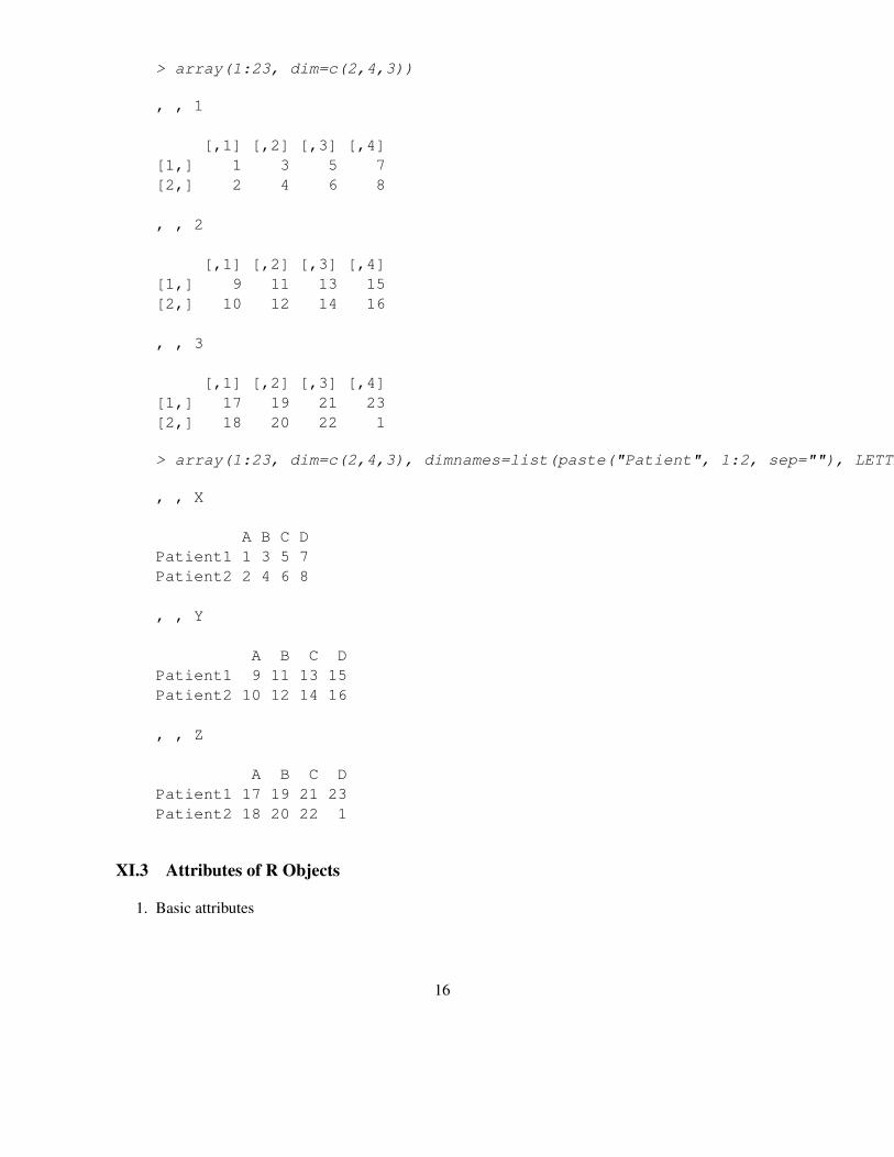
• array An array in R can have one, two or more dimensions. I find it useful to store multiplerelated data.frame (for example when I jack-knife or permute data). Note if there are insufficientobjects to fill the array, R recycles (see below)

> array(1:24, dim=c(2,4,3))

, , 1

[,1] [,2] [,3] [,4][1,] 1 3 5 7[2,] 2 4 6 8

, , 2

[,1] [,2] [,3] [,4][1,] 9 11 13 15[2,] 10 12 14 16

, , 3

[,1] [,2] [,3] [,4][1,] 17 19 21 23[2,] 18 20 22 24

15

> array(1:23, dim=c(2,4,3))

, , 1

[,1] [,2] [,3] [,4][1,] 1 3 5 7[2,] 2 4 6 8

, , 2

[,1] [,2] [,3] [,4][1,] 9 11 13 15[2,] 10 12 14 16

, , 3

[,1] [,2] [,3] [,4][1,] 17 19 21 23[2,] 18 20 22 1

> array(1:23, dim=c(2,4,3), dimnames=list(paste("Patient", 1:2, sep=""), LETTERS[1:4], c("X","Y", "Z")))

, , X

A B C DPatient1 1 3 5 7Patient2 2 4 6 8

, , Y

A B C DPatient1 9 11 13 15Patient2 10 12 14 16

, , Z

A B C DPatient1 17 19 21 23Patient2 18 20 22 1

XI.3 Attributes of R Objects

1. Basic attributes

16

The most basic and fundamental properties of every objects is its mode and length. Theseare intrinsic attributes of every object. Examples of mode are "logical", "numeric", "character","list", "expression", "name/symbol" and "function".

Of which the most basic of these are:

• ’character’: a character string

• ’numeric’: a real number, which can be an integer or a double

• ’integer’: an integer

• ’logical’: a logical (true/false) value

> x<-3> mode(x) # Numeric

[1] "numeric"

> x<-"apple"> mode(x) # Charachter

[1] "character"

> x<-3.145> x+2 # 5.145

[1] 5.145

> x==2 # FALSE, logical

[1] FALSE

> x <- x==2> x

[1] FALSE

> mode(x)

[1] "logical"

> x<-1:10> mode(x)

[1] "numeric"

> x<-LETTERS[1:5]> mode(x)

[1] "character"

17

> x<-matrix(rnorm(50), nrow=5, ncol=10)> mode(x)

[1] "numeric"

Repeat above, and find the length and class of x in each case.

2. Other attributes, dimension

> x <- matrix(5:14, nrow=2, ncol=5)> x

[,1] [,2] [,3] [,4] [,5][1,] 5 7 9 11 13[2,] 6 8 10 12 14

> attributes(x)

$dim[1] 2 5

In summary

Object Modes Allow >1 Modes*vector numeric, character, complex or logical Nomatrix numeric, character, complex or logical Nolist numeric, character, complex, logical, function, expression, ... Yesdata frame numeric, character, complex or logical Yesfactor numeric or character Noarray numeric, character, complex or logical No

*Whether object allows elements of different modes. For example all elements in a vector or array haveto be of the same mode. Whereas a list can contain any type of object including a list.

XI.4 Creating and accessing objects

We have already created a few objects: x, y, junk. Will create a few more and will select, accessand modify subsets of them.

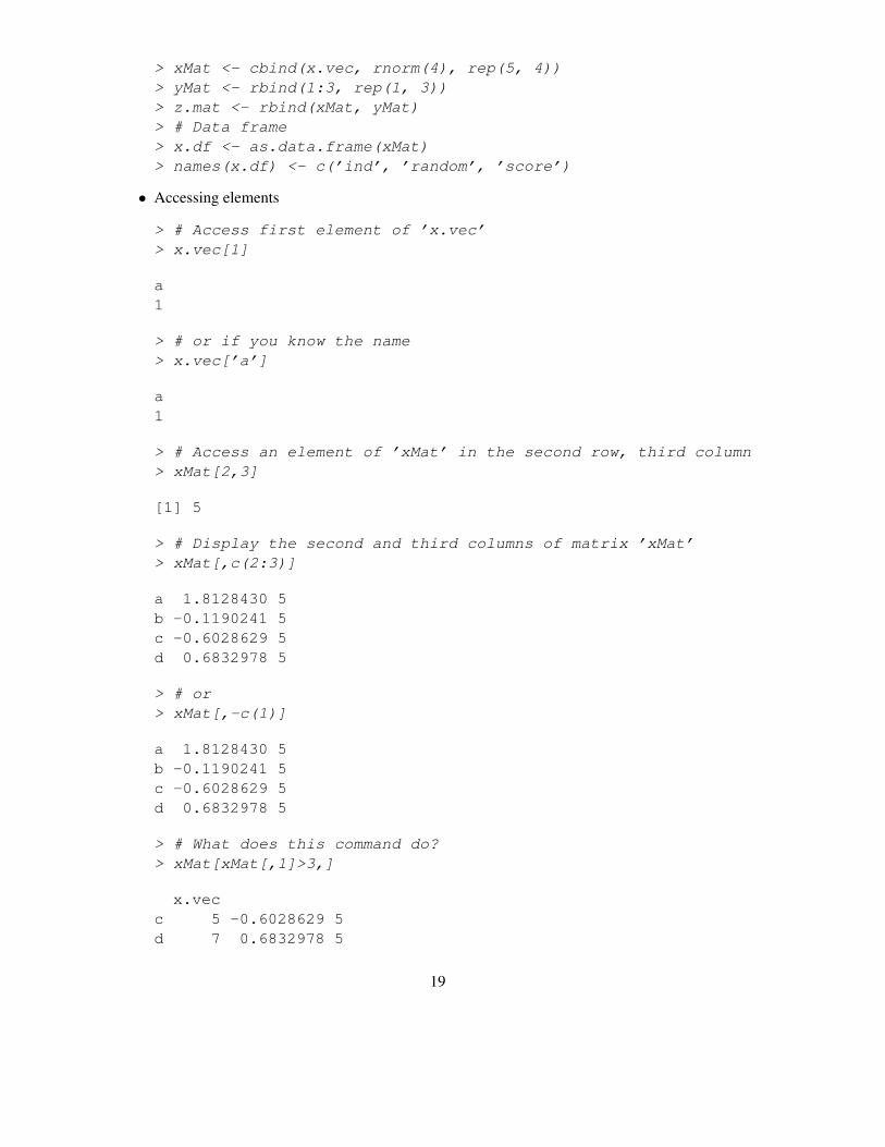
• Create vectors, matrices and data frames using seq, rbind and cbind

> # Vector> x.vec <- seq(1,7,by=2)> # The function seq is very useful, have a look at the help on seq (hint ?seq)>> names(x.vec) <- letters[1:4]> # Matrices

18

> xMat <- cbind(x.vec, rnorm(4), rep(5, 4))> yMat <- rbind(1:3, rep(1, 3))> z.mat <- rbind(xMat, yMat)> # Data frame> x.df <- as.data.frame(xMat)> names(x.df) <- c(’ind’, ’random’, ’score’)

• Accessing elements

> # Access first element of ’x.vec’> x.vec[1]

a1

> # or if you know the name> x.vec[’a’]

a1

> # Access an element of ’xMat’ in the second row, third column> xMat[2,3]

[1] 5

> # Display the second and third columns of matrix ’xMat’> xMat[,c(2:3)]

a 1.8128430 5b -0.1190241 5c -0.6028629 5d 0.6832978 5

> # or> xMat[,-c(1)]

a 1.8128430 5b -0.1190241 5c -0.6028629 5d 0.6832978 5

> # What does this command do?> xMat[xMat[,1]>3,]

x.vecc 5 -0.6028629 5d 7 0.6832978 5

19

> # Get the vector of ’ind’ from ’x.df’> x.df$ind

[1] 1 3 5 7

> x.df[,1]

[1] 1 3 5 7

XI.5 Modifying elements

> # Change the element of ’xMat’ in the third row and first column to ’6’> xMat[3,1] <- 6> # Replace the second column of ’z.mat’ by 0’s> z.mat[,2] <- 0

XI.6 Sorting and Ordering items

Sorting, might want to re-order the rows of a matrix or see the sorted elements of a vector

> # Simplest ’sort’> z.vec <- c(5,3,8,2,3.2)> sort(z.vec)

[1] 2.0 3.0 3.2 5.0 8.0

> order(z.vec)

[1] 4 2 5 1 3

> # Sorting the rows of a matrix> # We will use an example dataset in R called ChickWeight> # First have a look at the ChickWeight documentation (help)> #?ChickWeight> ChickWeight[1:2,]

weight Time Chick Diet1 42 0 1 12 51 2 1 1

20

> chick.short <- ChickWeight[1:36,]> chick.srt <- chick.short[order(chick.short$Time,chick.short$weight),]> chick.srt[1:2,]

weight Time Chick Diet13 40 0 2 11 42 0 1 1

> chickOrd<-chick.short[order(chick.short$weight),]

21

XI.7 Missing Values

Missing values are assigned special value of ’NA’

> z <- c(1:3,NA)> z

[1] 1 2 3 NA

> ind <- is.na(z)> ind

[1] FALSE FALSE FALSE TRUE

To remove missing values from a vector

> print(z)

[1] 1 2 3 NA

> x<-z[!is.na(z)]> print(x)

[1] 1 2 3

XI.8 Creating empty vectors and matrices

To create a empty vector, matrix or data.frame

> x1 <- numeric()> x2 <- numeric(5)> x1.mat <- matrix(0,nrow=10,ncol=3)

22

XII R sessions (workspace) and saving session history

To finish up today, we will save our R session and history

1. R session One can either save one or more R object in a list to a file using save() or save theentire R session (workspace) using save.image().

save(women, file="women.RData")save.image(file="entireL2session.RData")

To load this into R, start a new R session and use the load()

rm(women)ls(pattern="women")load("women.RData")ls(pattern="women")

2. R history R records the commands history in an R session. To view most recent R commands ina session

history()help(history)history(100)

To search for a particular command, for example "save"

history(pattern="save")

To save the commands in an R session to a file, use savehistory()

savehistory(file="L2.Rhistory")

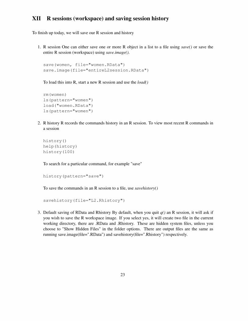
3. Default saving of RData and Rhistory By default, when you quit q() an R session, it will ask ifyou wish to save the R workspace image. If you select yes, it will create two file in the currentworking directory, there are .RData and .Rhistory. These are hidden system files, unless youchoose to "Show Hidden Files" in the folder options. There are output files are the same asrunning save.image(file=".RData") and savehistory(file=".Rhistory") respectively.

23

XIII Exercise 1

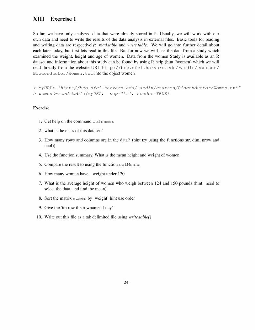
So far, we have only analyzed data that were already stored in R. Usually, we will work with ourown data and need to write the results of the data analysis in external files. Basic tools for readingand writing data are respectively: read.table and write.table. We will go into further detail abouteach later today, but first lets read in this file. But for now we will use the data from a study whichexamined the weight, height and age of women. Data from the women Study is available as an Rdataset and information about this study can be found by using R help (hint ?women) which we willread directly from the website URL http://bcb.dfci.harvard.edu/~aedin/courses/Bioconductor/Women.txt into the object women

> myURL<-"http://bcb.dfci.harvard.edu/~aedin/courses/Bioconductor/Women.txt"> women<-read.table(myURL, sep="\t", header=TRUE)

Exercise

1. Get help on the command colnames

2. what is the class of this dataset?

3. How many rows and columns are in the data? (hint try using the functions str, dim, nrow andncol))

4. Use the function summary, What is the mean height and weight of women

5. Compare the result to using the function colMeans

6. How many women have a weight under 120

7. What is the average height of women who weigh between 124 and 150 pounds (hint: need toselect the data, and find the mean).

8. Sort the matrix women by ’weight’ hint use order

9. Give the 5th row the rowname "Lucy"

10. Write out this file as a tab delimited file using write.table()

24

XIII.1 Cross platform tips

Use cross-platform file commands

> wkdir <-getwd()> newdir <-"MyNewDir"> newdirPath<-file.path(wkdir, newdir)> file.exists(wkdir)

[1] TRUE

> dir.create(newdirPath)> dir(pattern="My")

[1] "MyNewDir"

XIV Quick recap

• R Environment, interface, R help and R-project.org and Bioconductor.org website

• installing R and R packages.

• assignment <-, =, ->

• operators ==, !=, <, >, Boolean operators &, |

• Management of R session, starting session, getwd(), setwd(), dir()

• Listing and deleting objects in memory, ls(), rm()

• R Objects

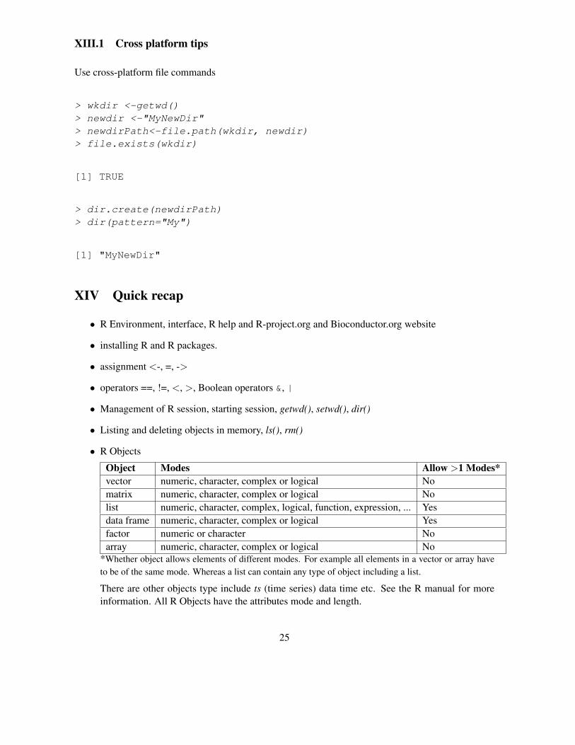
Object Modes Allow >1 Modes*vector numeric, character, complex or logical Nomatrix numeric, character, complex or logical Nolist numeric, character, complex, logical, function, expression, ... Yesdata frame numeric, character, complex or logical Yesfactor numeric or character Noarray numeric, character, complex or logical No

*Whether object allows elements of different modes. For example all elements in a vector or array haveto be of the same mode. Whereas a list can contain any type of object including a list.

There are other objects type include ts (time series) data time etc. See the R manual for moreinformation. All R Objects have the attributes mode and length.

25

• Creating objects; c(), matrix(), data.frame(), seq(), rep(), etc

• Adding rows/columns to a matrix using rbind() or cbind()

• Subsetting/Accessing elements in a vector(), matrix(), data.frame(), list() by element name orindex.

• Reading data into R using read.table()

• Saving an R session, R history

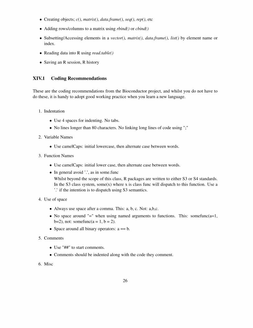
XIV.1 Coding Recommendations

These are the coding recommendations from the Bioconductor project, and whilst you do not have todo these, it is handy to adopt good working practice when you learn a new language.

1. Indentation

• Use 4 spaces for indenting. No tabs.

• No lines longer than 80 characters. No linking long lines of code using ";"

2. Variable Names

• Use camelCaps: initial lowercase, then alternate case between words.

3. Function Names

• Use camelCaps: initial lower case, then alternate case between words.

• In general avoid ’.’, as in some.funcWhilst beyond the scope of this class, R packages are written to either S3 or S4 standards.In the S3 class system, some(x) where x is class func will dispatch to this function. Use a’.’ if the intention is to dispatch using S3 semantics.

4. Use of space

• Always use space after a comma. This: a, b, c. Not: a,b,c.

• No space around "=" when using named arguments to functions. This: somefunc(a=1,b=2), not: somefunc(a = 1, b = 2).

• Space around all binary operators: a == b.

5. Comments

• Use "##" to start comments.

• Comments should be indented along with the code they comment.

6. Misc

26

• Use "<-" not "=" for assignment.

7. For Efficient R Programming, see slides and exercises from Martin Morgan http://www.bioconductor.org/help/course-materials/2010/BioC2010/

27