88
Introduction to Programming with Arrays using ELI by Wai-Mee Ching July, Nov., Dec. 2014 Copyright © 2014

Introduction to Programming with Arrays using ELI
by Wai-Mee Ching
July, Nov., Dec. 2014
Copyright © 2014
Contents 1. Array, List and Primitive Operations in ELI ......................................................................................................... 3
1.1 Computers and Programming Languages ............................................................................................................ 3
1.2 ELI System and its Data Types ............................................................................................................................ 6
1.3 Shape of Data, Reshape and Data Conversion ................................................................................................... 10
1.4 Mathematical Computations .............................................................................................................................. 13
1.5 Comparisons, Selection, Membership and Index of .......................................................................................... 17
1.6 Array Indexing, Indexed Assignment and taking Sections ................................................................................ 21
1.7 Array Transformations ....................................................................................................................................... 26
1.8 Operators and Derived Functions ...................................................................................................................... 31
1.9 Lists and Operations on Lists............................................................................................................................. 34
2. Defined Functions, Control Structures and Files ................................................................................................. 38
2.1 Defined Functions, Short-Form and Order of Evaluation .................................................................................. 38
2.2 One-liner Functions .......................................................................................................................................... 41
2.2.1 number conversion and lexicographic ordering .......................................................................................... 41
2.2.2 a queuing network model ............................................................................................................................ 44
2.3 Control Structures .............................................................................................................................................. 46
2.4 Recursion .......................................................................................................................................................... 47
2.4.1 sorting ......................................................................................................................................................... 47
2.4.2 tower of Honoi ............................................................................................................................................ 50
2.4.3 determinant ................................................................................................................................................. 51
2.5 Script Files ......................................................................................................................................................... 52
3. Array Implementation of Data Structures ............................................................................................................... 54
3.1 Emulation of PASCAL Data Structures in ELI ................................................................................................. 54
3.1.1 a small database for a company .................................................................................................................. 54
3.1.2 implementation of linked lists in ELI ......................................................................................................... 58
3.1.3 implementation of queries to a database ..................................................................................................... 61
3.2 Binary Trees ..................................................................................................................................................... 63
3.2.1 tree representation ....................................................................................................................................... 63
3.2.2 tree operations ............................................................................................................................................. 65
3.2.3 tree transversals .......................................................................................................................................... 68
3.3 Quad Trees ........................................................................................................................................................ 70
3.4 Graph Algorithms ............................................................................................................................................. 72
3.4.1 graph representations .................................................................................................................................. 72
3.4.2 depth first search ......................................................................................................................................... 73
3.4.3 single-source source shortest path .............................................................................................................. 74

4. Computational Algorithms ..................................................................................................................................... 77
4.1 Iterative Method ................................................................................................................................................ 77
4.2 Simple Encryption and Monte Carlo Method .................................................................................................... 79
4.3 Sparse Matrix Computation ............................................................................................................................... 82
References.................................................................................................................................................................... 85

1
The process of preparing programs for a digital computer is especially attractive, not only because it can be
economically and scientifically rewarding, but it can be an aesthetic experience much like composing poetry or
music.
-D. Knuth, the Art of Programming
By relieving the brain of all unnecessary work, a good notation sets it free to concentrate on more advanced
problems, and in effect increases the mental power of the race.
-A.N. Whitehead, quoted in Ken Iverson’s Turing Lecture
Preface
The mathematician and computer scientist Jacob T. Schwartz once remarked that programming (and
programming languages) consists of two sides: internal and external. The internal side is of a mathematical nature
concerning the algorithmic transformation of data. The external side is of a mundane nature concerning system
interface and human factors. In the programming language APL, designed by Ken Iverson, language idiosyncrasies
arising from the external side have been kept to a bare minimum so a programmer can concentrate his effort on the
algorithmic side of a programming job, and its programming environment is particularly simple. APL treats arrays
as its primary data structure, and provides a comprehensive set of array operations as language primitives each
denoted by one character in a special font (APL font). As Alan Perlis once pointed out APL encourages a dataflow
style of programming, i.e. organizing tasks in chains of functions and operators on arrays, or what we call array-
oriented programming. This combination of succinct notation and powerful primitives allows an APL programmer
to have a clearer global view of his programming constructs than in any other language, with the possible exception
of SETL, since many low level details have been suppressed.
While the APL font used to denote primitives achieves succinctness with exquisite beauty it presents
difficulties for input/output, exchange of code segments in mails, and APL systems often do not communicate easily
with ASCII-based text files. ELI is an array programming language based on APL where primitive operations are
denoted by one or two ASCII characters thus maintaining the one-character one symbol principle of APL to
preserves APL’s dataflow style in array-oriented programming. ELI has the same programming environment
centered on a workspace as that in APL, it also makes input/output of ASCII-based text files containing code as well
as data much easier. ELI has all the language features of the classical APL [9]; it does not have the general array
feature of APL2 [13] but it provides lists and basic operations on lists to deal with irregular or non-homogeneous
data. In addition, ELI supports complex numbers, symbol type and temporal data.
Any discussion of program design inevitably brings up the question of efficiency. There are actually two
different kinds of efficiency which are of concern here: the human programming efficiency and the machine
execution efficiency. In other words, we like to know how quickly a working program can be implemented, and how
fast that program will run. At the heart of execution efficiency is the choice of algorithm(s) used for a programming
task as the design and analysis of algorithms is at the foundation of computer science [8]. However, we assume here
that an efficient algorithm is already chosen which is appropriate for given circumstance in terms of likely input data
size or time limit for implementation (the asymptotic efficiency of worst-case behavior of an algorithm may not be
as important as the average performance of an algorithm, and one may trade a more efficient algorithm with a less
efficient one in order to avoid implementation complexity). With this assumption, the execution efficiency of a
program then largely depends on the efficiency provided by the language processor deployed in the process. And
clearly there is a trade-off between the pursuit of execution efficiency and that of programming efficiency for each
programming job. For example, one may choose to use MATLAB to solve an engineering problem instead of using
FORTRAN. On the other hand, for a problem which will likely result in long running time, one will consider using
FORTRAN instead of MATLAB seriously. There are two camps of programming languages, those based on

2
interpreters and those based on compilers, i.e. interpretative languages and compiled languages. In general, it is
faster to develop programs in an interpretative language than in a compiled language, but a compiled program
typically run much faster than its counterpart written in an interpreted language.
Iverson intended APL to be a tool of thought for communicating algorithmic ideas precisely (see his Turing
Award Lecture [10]); consequently, APL, with mathematically inspired notations and high-level primitives, is
remarkably productive in turning algorithmic ideas into programs. Arthur Whitney, developer of A+ at Morgan
Stanley (www.aplusdev.org) and kdb (www.kx.com), once remarked that often the true productivity factor provided
by APL is not 5 or 10 but infinity because some complex systems written in APL/A+ would never have reached
operational state had some conventional language been chosen to implement it. APL is also quite versatile as it has
been used profitably in areas ranging from finance, actuarial, computer-aided design, logistics manufacturing, and
research in physics, econometrics and biometrics. ELI inherits these strengths of APL. Finally, while APL
programs incur the inefficiency of an APL interpreter, ELI system provides a translator (covering most array portion
of ELI) to turn an ELI program into a C program to be compiled, thus avoids the execution inefficiency of its
interpreter [2].
Any reader who has the patience to go through a good portion of this introduction to programming with
arrays will discover that ELI is fairly easy to learn. No prior knowledge of APL or programming experience in
another programming language is required. In fact, this book is quite suitable for people who have never taken a
class in programming but intend to learn serious programming with only a basic background in mathematics. For
people who are already familiar with some popular programming languages such as C, Java, we point out that in
C/C++ or Java a program is mostly organized around loops; in contrast, a program in APL/ELI is best organized as
chains of powerful primitives manipulating arrays. This suppression of details not only results in elegant APL/ELI
programs but also eliminates a lot of low level cleric errors in programming. Moreover, such a source program is
ideal for automatic parallelization [6] by a parallelizing compiler on multi-core machines. Finally, one must have
programmed in APL/ELI to fully appreciate the ingenuity of Iverson in designing APL: its economy of notations,
innovative treatment of limiting cases and remarkable mathematical consistency. As ELI is freely available on
multiple platforms, we hope this introduction will attract more people to experiment with ELI and come to realize
that programming with arrays can indeed be an aesthetic experience much like composing poetry or music, and that
a clean notation indeed sets our brain free to concentrate on more advanced problems.
Mount Kisco, NY, 2014.

3
1. Array, List and Primitive Operations in ELI
1.1 Computers and Programming Languages
A computing device is some object which can carry out computations reliably. Today such devices range
from smartphones, tablets, personal computers, servers to supercomputers. For simplicity, we call all these
computing devices computers. A basic computer consists of three units: central processing unit (CPU), memory and
input/ output unit (or simply I/O); this is the classical von Neumann machine. Today, a parallel computer’s
processing unit can starts from multi-core processor to multi-processors, and there are shared-memory parallel
computers as well as distributed-memory parallel computers with various inter-connection networks. An input
device can be a touch screen or a keyboard; an output device can be a liquid crystal display or a laser printer. The
memory unit is where a computer stores users’ programs and data. The CPU fetches an instruction-stream from the
memory, decodes it, i.e. figures out the meaning of the instructions, which may include fetching data from memory,
and carries out its execution in an appropriate order. Each computer understands only a fixed set of instructions in
binary form, i.e. some particular sequences of 0’s and 1’s. For example, an Intel-based PC understands the Intel x86
Instruction Set. This set of instructions constitutes the machine language of an Intel-based computer.
It is certainly extremely tedious and error-prone to prepare a program in the machine language of a computer.
So the first thing people did was to introduce assembly languages. An assembly language for a particular type of
computer is basically the same as the machine language of that class of computers except for the following two
points: First, mnemonics are used to represent operation code instead of their binary format. For example,
A
means the add integer instruction instead of the binary string
01011010
which the machine (an IBM 370) understands. Second, labels are introduced to denote a certain place for an
instruction, and names are introduced to represent numbers which are memory locations. For example, if
L1: A 1,2
is the 99-th instruction in a program, an instruction
B L1
will branch to that instruction without specifying that the instruction with label L1 is the 99-th instruction.
The memory of a computer can be visualized as a contiguous array of numbered boxes (i.e. each box has an
address), each containing a binary data of 8 bits (a bit is the basic electronic entity and can be either on or off to
represent a binary digit of 1 or 0). Such a box is by custom called a byte. Memory in a computer usually is only
addressable by words; a word can be either 4 bytes or 8 bytes. A byte can have 256 different configurations and can
therefore be used, via some encoding scheme, to present a set of 256 characters. For example, in a commonly used
encoding system called ASCII the character ‘A’ is represented by
01000001
Usually, an integer is represented in its binary form in a word with the first bit indicating the sign. For example, 3
and -2 are represented in 32-bit word by
00000000000000000000000000000011

4
11111111111111111111111111111110
respectively. Numbers with possible fractional parts are represented differently in floating-point format which we
will not get into here. Besides characters and numbers, a byte or a word of data can represent other entities through
various representation schemes.
The CPU of a typical computer consists of a control unit, an instruction decoder, an address generator, a
program counter, arithmetic and logic unit (ALU), a program status word (PSW) which is used to record the state
of the machine and is saved when machine execution is interrupted, part of PSW is called condition code, and
several general purpose registers denoted as
R0, R1, …, R15
The registers are simply data storage places (16 in IBM 370 with 32 bits each) located in CPU. The
execution of a program, i.e. a sequence of machine instructions is as follows:
1. Fetch the next instruction to CPU and increase the program counter so it points to the next instruction (adds
4 if each instruction is 4 bytes long).
2. Decode the instruction.
3. If the instruction involves data from memory then fetch the data at the memory location pointed to by the
address generator.
4. Execute the instruction and go back to step 1.
Soon after assembly languages were created, people discovered that it was helpful to introduce a convention so
that a short-hand notation like an assembly instruction can replace a repeatedly used sequence of code, with possible
variation of data. This is an assembler with macro-facility. Life is made a bit easier, but it is still quite a burden if
you always have to keep track of registers and memory locations during programming.
Finally, people introduced high-level programming languages. Instead of operating on registers and memory
locations, variables are used for data items. Consequently, program statements can be written more like ordinary
mathematical computations. But machines do not understand any of the high-level languages. So people write
programs to bridge the gap between the machine (or assembly) languages and various high level languages. Such
programs are called language processors. Among high level programming languages, there are, like computers,
general purpose programming languages designed for a variety of applications, and special purpose languages
designed for some specific application areas. We shall only talk about general purpose programming languages.
There are two kinds of programming language processors: compilers and interpreters. A compiler COMP for a
programming language L for a machine M accepts a program p[L] written in programming language L as an input to
COMP, and transforms p[L] into a semantically equivalent program p[Ml] written in the assembly language Ml of
computer M as the output of COMP.
COMP: p[L] -> p[Ml]
The program (text) p[L] is usually called the source code while p[Ml] is called the compiled code which can
further be turned into object code o[Ml] of machine M by an assembler for Ml. When we run o[Ml] on machine M, it
would accept what p[L] would accept as input and carry out operations specified in p[L] including production of
outputs.
An interpreter of a programming language L for a machine M, on the other hand, is a program INTP which
accepts a program p[L] written in L, one unit (usually an expression in that language) at a time, and carries out
immediately what was semantically specified in that unit until the whole program p[L] has been processed.
Languages whose processors are primarily compilers are called compiled languages; languages whose processors

5
are interpreters are called interpreted languages. The division becomes less clear when some compiled languages
offer interpreters and some interpreted languages acquire compilers. A compiled language typically requires a
programmer to declare in the beginning of his program all variables (and their types) to be used in his program
while interpreted languages usually do not have such a requirement.
Examples of important compiled programming languages are:
• FORTRAN, the first high-level programming language, and still used in scientific community today.
• COBOL, most used programming language for commercial data processing for a long while.
• PASCAL, invented for structured programming and enforces strict typing.
• C/C++, C is the most commonly used system programming language and serves as a common assembly
language; C++ is based on C but incorporating object-oriented programming features.
• ADA, a language based on PASCAL and promoted by US Department of Defense.
• Java, an object-oriented language designed to run on a wide range of computing/communication devices.
Examples of interpreted programming languages are, with each of its descendants in parentheses:
• BASIC (Visual Basic), a simplified version of FORTRAN, designed for easy learning and widely available.
• Lisp (Common Lisp, Scheme), a list based programming language used widely in artificial intelligence area.
• APL (APL2, J, Q, ELI), an array oriented programming language with succinct symbols.
• MATLAB (Scala), it is functionally similar to APL, but with FORTRAN like syntax.
• Perl, started as a language for text processing and become very popular for shell language like system work.
• Python, it is similar to Perl but with good vector processing capability.
• Ruby (Ruby on Rails), it is a programming language popular for writing web applications.
• Haskell, a functional programming language with static typing.
Strictly speaking, Java is interpreted, i.e. a Java program is compiled into a sequence of Java Virtual Machine
(JVM) code, and that sequence of JVM code is then interpreted. As JVM is implemented on different machines and
communication devices differently, the compiled JVM code for a particular Java program remains the same. In fact,
a Perl program is also not interpreted line by line but compiled into an internal form which is then interpreted. The
reason we listed Java in the compiled camp is because its programs required variable declarations similar to that in C.
In the case of Perl, variable declaration is not exactly required. On the other hand, there exists working compiler for
(classical) APL ([3],[5]), though not commercially available; and we do have a compiler which covers a large
portion of the ELI programming language available [2]. Thus, ELI would provide both the programming
convenience and productivity of an interpreted language as well as the execution efficiency of a compiled language
for large portion of its programs. MATLAB also offers a compiler to produce code which can be executed
independent of its interpreter environment if not necessary to provide higher execution efficiency.
We remark that many compiled languages nowadays provide Interactive Development Environment (IDE) to
make their coding/debugging process more like that of an interpretive language. The most well-known IDE may be
Microsoft’s Visual C++, now part of Visual Studio covering other languages such as Basic. Still, interpretive
languages, by saving the compilation step and skipping elaborative declaration in a program, provide appreciable
programming productivity over compiled languages while suffer in execution efficiency. For many non-product
application software, this is understandably a good trade-off; and further efforts in providing compilation capability
for some interpretive languages just make this trade-off more attractive.
There are two ways to envision about how to structure a (large) program: the top down approach and the bottom
up approach. The top down approach is best exemplified by the object-oriented programming model while the
bottom up approach is best exemplified by very high level programming languages, i.e. incorporating frequently
used operations on main data structures such as arrays into very high level language primitives. C++ and Java are in

6
the first camp while MATLAB and APL/ELI are in the second camp. There are also attempts to combine the two as
shown by Scala, an open source descendent of MATLAB.
The design philosophy of Ken Iverson on APL is that of simplicity. APL is powerful in the sense expressed by
Conrad Barski in Land of Lisp: “To make a programming language powerful, you need to make it expressive.
Having an expressive language means that you can do a lot of stuff with very little actual code”. This approach
applies not only to the economy of notation in language syntax but also in having only a few organizing concepts for
the language. This is in sharp contrast with that of object-oriented programming model where one has to learn
classes, methods, inheritance etc. before any meaningful example can be discussed. Admittedly, complex (system)
applications need object-oriented programming model to develop and maintain manageable code, but many
programming jobs do not really need such elaborate conceptual prerequisites to accomplish a job at hands.
Moreover, APL and its descendants have been used to implementing huge systems in chip design, manufacturing
logistics, financial databases with time series and derivative trading systems. ELI adopts all minimalist design
principles of APL. ELI has made only one pragmatic compromise with respect to APL, i.e. it uses ASCII characters
in lieu of the special APL character set in order to have easier exchange of code and data through e-mail or file
input/output. Still, by replacing each APL character with one or two ASCII characters, ELI has essentially
maintained the one-character one-symbol spirit of APL language. On the other hand, ELI has added list, dictionary
and table to ISO APL [9] to enhance its power in handling non-homogeneous data and make it more convenient for
doing large data analysis.
1.2 ELI System and its Data Types
Once you downloaded ELI and installed it on your computer, if it is a Windows system, just put eli.exe in your
desktop or some other directory. Click on the eli.exe icon and you see a window pop up with the following lines:
ELI version 0.2 (C) Rapidsoft
CLEAR WS
For Linux or Mac OS platform, after you put elix (elim for Mac OS) in a directory of your choice, cd to that
directory and type ./elix, you see the same two lines response as the above except that there is no GUI window as
ELI is command line based for Linux and Mac OS.
Now you are in ELI, i.e. you entered the ELI programming environment. To get out this ELI environment after
you finish doing programming or experimentation, simply type
)off
then you would be back to the host system, be it Windows, Linux or Mac OS. ELI, as in APL, provides workspaces
as a basic organizing unit for programmers to develop, debug, save and load his (saved) programs. A workspace
consists of stored data (variables) and (user defined) functions as well as errors encountered in running expressions
(portions of a program). CLEAR WS indicates it is a clear workspace meaning that it is a clean slate to work on, i.e.
there is nothing there, except some pre-existing system variables provided by the ELI system. One of such system
variable is []IO, the index origin, which can be either 1 or 0. Type []IO
1
You type again (the lines displayed with an indentation), and you see the system responses with a line:
!10
1 2 3 4 5 6 7 8 9 10

7
where ! is the interval function which generates a vector of n integers from 1 or 0 depends on []IO. We can
change the value of []IO by an assignment and see its effect on !:
[]IO<-0
!10
0 1 2 3 4 5 6 7 8 9
Hence, for []IO= 0, it is just like in C. Later we’ll see that there are other primitive operations such as indexing
which also depend on []IO. Continue to explore, we type in
100+!10
101 102 103 104 105 106 107 108 109 110
v<-100+!10
v
101 102 103 104 105 106 107 108 109 110
w<-2*v
w
202 204 206 208 210 212 214 216 218 220
We notice two things: i) ELI code operates from right to left and ii) value created can be stored into a variable by an
assignment (<-). Now, if we type
a
value error (* system response *) a
^
This is because a variable named a has not been assigned any value yet. A variable name must start with an
alphabet, then possibly followed by alphanumerical characters and the ‘_’ character (but ‘_’ cannot be the ending
character). For example, ab12_99, Acx, h_103 are legitimate variable names while 0ac and u55_ are not. Once
a variable is created by an assignment, its value can be further used in later operations:
2+a<-1
3
We note the assign symbol <- is a two character symbol while =, which represents the symbol for assignment in
some programming languages, is the symbol for the equality function in ELI. Symbols which represent primitive
functions, i.e. operations provided by the ELI system, consist of either one or two ASCII characters. For a two
character symbol such as assignment no blank character is allowed in between. Let us continue our exploration:
b<-'A'
b
A
b+1
domain error
b+1
^
This is because variable b has a value which is of type character and arithmetic operations are not defined on data of
character type. Here, by data we refer to either literal data, i.e. data directed represented the item as written, or
variables or expressions holding values of various types.
ELI has four basic types of data: numbers, character, symbol and temporal data. We have just seen numeric and
character data. Symbolic data are like (variable) names affixed with a back tick such as
`a1 `aapl `goog
The system variable []TS gives the current time which is a temporal data of type datetime:

8
[]TS
2013.07.14T00:04:54.332
while 2013.07.14 is of type date and 00:04:54 is of type second. Altogether there are six subtypes of temporal
data type (see [4] sect. 2.4).
There are four subtypes of numerical data: boolean, integer, floating point and complex numbers, in an
expanding order; boolean data consists of only 0 and 1 which represent false and true respectively. A boolean is
also an integer, an integer can be used where a floating point number can be used and a floating point number can be
used where a complex number can be used. A negative number is affixed with the ‘_‘ character:
2–1 2 3
1 0 _1
To write a negative number the ‘_’ character must immediately be followed by a digit; it is treated similar to the
‘.’ point in a number. Numbers are written in decimal form
24 _1.2 0.2 3.0 .5
are all legal representation of numbers in ELI except the last one since there must be a 0 before ‘.’ for a fractional
number less than 1 in ELI. For scaling, both ‘e’ and ‘E’ are acceptable:
1.2e2
120
1.2E_2
0.012
A complex number is of the form RjI, where R is the real part and I is the imaginary part, each written as an
integer or a floating point number and there should be no space before or after j. For example the square root of _1
is
_1*.0.5 0j1
2j5+3j2.5
5j7.5
2j5*3j2.5
_6.5j20
We note that ELI does not make an explicit distinction between floating point numbers and fixed point numbers.
In other word, in ELI one does not concern about how a number is represented in the machine. An integer is an
integral number which may be represented in floating point format in the machine by the system if it is too large.
As we have seen already literal character data is a string of characters quoted by a pair of quotation marks as in
the assignment above to variable b. But when ELI displays the value of b the quotation marks are taken away. To
represent a quotation mark, we need to use a double quotation:
ch<-'abcd''e''1234'
ch
abcd'e'1234
The functions provided by the ELI system which operate on ELI data are called primitive functions. We have
already seen a few primitive functions: ! (interval generator), + (addition), * (multiplication) and *. (power or
exponent). A primitive function is called monadic if it takes one (right) argument or dyadic if it takes two

9
arguments, i.e. a left and a right argument. Some primitive functions apply to data of any type, and some primitive
functions apply only to data of certain type. For example, ! applies only to non-negative integers while = applies
to a pair of any data.
'A'=b
1
1=b
0
When a primitive function applies to improper data, i.e. where it is not defined, it results in a domain error.
ELI has two modes of operation: execution mode and function definition mode. What we have seen is the
execution mode: you type in some ELI expression, the system responses either with an answer or an error message.
This is why systems like ELI are called interactive, or interpretive. The system is in function definition mode when
you start to create and edit a user defined function (also called procedures in languages like C). We’ll come to that
in the next chapter. One can also prepare function text and other expressions in a file outside of the ELI system
using an ordinary text editor and then load that file into the ELI system (see chapter 2).
ELI system recognizes two broad classes of instructions: ordinary ELI expressions dealing with the algorithmic
calculations/transformations of data in an active workspace, and system commands. We can look at an ELI system
as consisting of two components: a supervisor and an interpreter. The supervisor is the broker between the ELI
programmer and the outer environment, i.e. the operating system of a machine (Windows, Linux or Mac OS) where
the ELI system is situated. It takes care of the initiation and termination of an ELI work session (the )off command),
saving and loading saved copies of workspaces; loading files and transferring data and functions to files. The
interpreter parses and executes an ELI expression, and its result for which we have just seen few examples. One of
the system commands is to change, or give a name to the clear workspace we have been working on:
)wsid abc
by that we give the name abc to the active workspace, the other is
)save
Note that a clear workspace cannot be saved; it must have a name. A saved workspace can be loaded later by
)load abc
The system command
)vars
will list all user defined variables in the current workspace, and the command
)vars a
will list all user defined variables whose name starting with a in the current workspace; the system command
)fns
will list all user defined functions in the current workspace, and the command

10
)fns a
will list all user defined functions whose name starting with a in the current workspace. There are other system
commands (see [4]).
1.3 Shape of Data, Reshape and Data Conversion
A single data item such as a number, a character of a symbol and a variable which is assigned such a value is
called a scalar while a group of items of the same type, or a variable holding such a value, is called an array. For
example, 1 is a scalar and the variable b in the previous section is holding a scalar value while the variable ch and
(the result of)!9 are one dimensional arrays. To know the shape of (literal) data or a variable, we apply the monadic
primitive function #, called shape of, to the data or variable in question. The shape of a scalar (say variable b above)
is an empty vector
#b
(* system response is a blank indicating an empty vector *)
i.e. scalars have no shape just like points have no length. There are two ways to write a literal empty vector:!0
or ’’. What is the shape of an empty vector?
##b (* we ask the shape of #b *) 0
#!0
0
’’=!0
(* system response is a blank indicating an empty vector *)
Hence, the system says the shape of an empty vector is a vector of length 0. Note that the response to our question of
whether ’’ equals to !0 is neither true (1) nor false (0) but an empty vector. This may seem to be a surprising
choice until we understand that the primitive function ‘=’ requires both arguments to have the same shape S (or one
side is a scalar, as we will explain in more detail later) and its result is always of the same shape as that of S.
A one dimensional array is called a vector, a two dimensional array is called a matrix and there are arrays of
higher dimensions. All elements in an array must be of the same type, i.e. they are either numeric, character,
symbolic or temporal. For a vector v, the shape of v is its length.
#a<-1 3 7 9 4
#C<-‘abcde’
5
We see from the above that to denote a numeric vector we only need one or more spaces to separate the numbers
which are the individual elements of the vector; and to denote a character vector we write it as a quoted string with
no space in between unless we want to include blank characters. If we have
a
1 2 3
4 5 6
then

11
#a
2 3 (* system response *)
i.e. a is a matrix of 2 rows and 3 columns. If ec is the following 3-dimensional array
ec
abcd
abcd
abcd
abcd
abcd
abcd
then
#ec
2 3 4
In general, for an array a, #a is a vector sv whose elements are the lengths of a in each dimension, the axis. For
a matrix, the first dimension runs from top to bottom and the second axis runs from left to right. ##a, i.e. the shape
of the shape vector of a, is called the rank of a, which is the dimension of a.
There is a monadic primitive function count ^, for which ^w gives the number of elements in w, and for a scalar w,
^w is 1 (this saves us the need to ravel a scalar in cases for counting purpose). So we have,
^ec
24
^`abc
1
^’abcd’
4
A convenient way to produce some numeric vector in ELI is to use the monadic primitive function ! called
interval generator:
!10
1 2 3 4 5 6 7 8 9 10
It gives a vector of 10 integers starting from 1 if []IO is 1 (or starting from 0 and ending in 9 if []IO is 0 ).
Another way to generate vectors is to use the dyadic primitive function # called reshape
10#’a’
aaaaaaaaaa
A primitive function symbol is called ambivalent if it denotes either a monadic or dyadic function, i.e. having one or
two arguments. In ELI, for economy of symbols and conciseness of notation, a one-character (or two-character)
symbol usually represents two primitive functions: one monadic and one dyadic, depending on whether there is only
one argument to the right of that symbol or there are two arguments, i.e. with an additional argument to the left of
the function symbol. So, #a is the shape of a while s#a is the reshape of a into an array s#a of shape s, where s is
a non-negative integer or a vector of non-negative integers. For example,
a<-3 4#!10
a

12
1 2 3 4
5 6 7 8
9 10 1 2
#a
3 4
2 3 4#'abcd'
abcd
abcd
abcd
abcd
abcd
abcd
0#a
(* system response is a blank line indicating an empty vector *)
i.e. an empty vector, because 0 is the shape of an empty vector;
3#’abcd’
abc
We notice that the reshape function # use the elements of its right operand to form an vector/array whose shape
is specified by the left operand. In case there are not enough elements to go around, it would reuse previously
appeared elements (hence a convenient way to generate many copies of a data item is to reshape it); and in case
there are more elements than needed, it only takes the amount it needs. In summary, we have
#s#a �� s
namely, the shape of the result of a reshape is the left operand of the reshape. In ELI there are many such identities
which help one to reason about a program. Let sx<-10 and vx<-1#sx then #sx is an empty vector while #vx is 1,
but both ^sx and ^vs are 1. Hence, in some situations the count function ^ is more convenient to use.
There is a monadic primitive function format +.a which will turn its numeric or symbolic operand a into its
character representation:
+.a<-12.3
12.3
^a
1
^+.a
4
+.as<-`abc `b1
abc b1
#as
2
#+.as
6
Conversely, if we have a character string s which represents a number or a symbol then the execute function !.s
will turn it into a number or symbol:
2+!.'12.3'
14.3
5#!.'`abc `b1'
`abc `b1 `abc `b1 `abc
The function !. is actually far more powerful; it takes in a character string and executes it as a line of ELI code.

13
1.4 Mathematical Computations
ELI has a rich set of primitive functions, i.e. more than the usual four arithmetic functions found in most
programming languages, with additional ones coming from something like a standard math library. There are two
kinds of primitive functions in ELI: scalar and mixed. A scalar function has the characteristic that when f is
applied to an array, it is an extension of f‘s application to each element of the array for monadic f. For dyadic f, its
two arguments must be conformable, i.e. either both are of the same shape, or one of them is a scalar or a one
element vector, in which case that argument is reshaped to the shape of the other argument before function
application. Suppose we have
b
1 2 3 4
c
5 6 7 8
b+c
6 8 10 12
100+b
101 102 103 104
a
1 2 3
4 5 6
d
12 11 10
9 8 7
a+d
13 13 13
13 13 13
c
1 1
1 1
1 1
a+c
length error (* because a and c do not have the same shape *)
a+c
^
Two more examples:
-1 2 3 4 _1 _2 _3 _4
5-1 2 3 4
4 3 2 1
Note that the monadic negation function applies to every element of the right argument and produces a vector of 4
negative numbers.
There are three groups of scalar functions: arithmetic, logical and relational. The arithmetic functions are
monadic symbol dyadic
conjugate + add
negative - subtract
signum * multiply
exponential *. power
reciprocal % divide
natural logarithm %. general logarithm
pi times @ circle functions

14
absolute value | residue
floor _. minimum
ceiling ~. maximum
roll ?. deal (a mixed function)
factorial |. binomial(mixed function)
The domain of a primitive function f is a data (sub-)type where f is well-defined. For example, shape(#) is defined
for all data types while monadic ! is defined only for non-negative integers. The domain of arithmetic functions is
numeric data in general, but further restrictions on some functions are required. A numeric function always yields a
numeric result. We refer to [4] for a detailed description of these functions. We shall give some examples of the
use of these functions besides the ones we have already encountered.
Let a and b be literal numeric data or variables having numeric value in the following examples. a*b is the
product of a and b. while a*.b is a to the power of b.
2*0 1 2 3 4 5 6 0 2 4 6 8 10 12
2*.0 1 2 3 4 5 6
1 2 4 8 16 32 64
We have already seen that –a is 0-a while %a is 1%a.for a numeric a, scalar or array. We note that - is the inverse
function of + while % is the inverse function of * and 0 is the identity element of + (i.e. it is neutral to the operation:
0+a=a for all a) while 1 is the identity element of * (i.e. 1*a=a for all a). 2*.0.5 is 1.414213562, the square
root of 2, and we can compute cube root, 4th
root etc. similarly:
%1 2 3 4 5 6
1 0.5 0.3333333333 0.25 0.2 0.1666666667
64*.%1 2 3 4 5 6
64 8 4 2.828427125 2.29739671 2
We state here the most important rule in evaluating an ELI expression: evaluation is from right to left in the
sense that the result of an operation on the right feeds as an input to the next operation, and all functions have equal
precedence but in case the left operand of a dyadic function is in parentheses then what inside the parentheses must
be evaluated first. Hence,
2*3+10
26
(2*3)+10
16
Back to computing various roots of a number, we calculate reciprocals of a sequence of numbers first and then apply
the power function. This is actually a special example of taking fractional exponents (powers). Next
_1*.0.5
0j1
as we know that square root of _1 is the complex number i. A complex number is written in the form RjI where R
is the real part and I is the imaginary part. Note that no blanks are allowed before or after j and what follows j
must be part of a literal number, but if I is 0 then it reverts back to real number form. For two complex numbers,
R1jI1+R2jI2 equals to R3jI3 where R3=R1+R2, I3=I1+I2 and R1jI1*R2jI2 equals to R3jI3 where R3=(R1*R2)-I1*I2, and I3=R2I1+R1I2

15
2j5+3j2.5
5j7.5
2j5*3j2.5
_6.5j20
The monadic + function conjugate when applies to a complex number RjI results in RjIn withere In=-I :
+_1*.0.5
1
+_1j0.5
_1j_0.5
We’ll introduce the derived function sum of a vector v here as +/v:
+/!100
5050
+/v<-_1 2 3 6.8 10
20.8
For a vector (x;y;z) in 3-dimensional space, the length of this vector is square root of (x2+y
2+z
2). Hence if a vector
v in ELI of n elements is representing a vector in n-dimensional space, then its length is calculated as
(+/v*.2)*.0.5 12.65859392
for the v above. However, for a vector u in a complex n-dimensional space the length is computed a square root of
the sum of u*(u*) , where u* is the conjugate of u. For example,
u<-0j1 1j2 4
(+/u*+u)*.0.5
4.69041576
The monadic * function signum when applies to a real number R results in
1 if I>0; 0 if I=0; _1 if I<0
Suppose P is the prices of a stock trades in the first minute of market opening, P0 (=20) is the closing price of that
stock in the previous day. Now we can see easily which are up-trades and which are down-trades:
P
17.3 22.3 24.3 17.5 21.4 18.4 17.2 15 20.8 21.8
*P-P0<-20
_1 1 1 _1 1 _1 _1 _1 1 1
and this result can be used further for other purpose as we’ll see later. We remark that the signum function is also
defined for complex numbers but we are not going to explain here this mathematical extension.
The monadic function *. is the mathematical exponential function.
eu<-*.1
eu
2.7182818
*. _1 0 1 2 3
0.36787944 1 2.7182818 7.3890561 20.085537
eu*. _1 0 1 2 3

16
0.36787944 1 2.7182818 7.3890561 20.085537
We see that eu above is the famous mathematical constant (a transcendental number) e, also called the Euler
number, and that *.v is just a convenient way to write eu*.v for any numerical (scalar or array) v.
The dyadic function a%.b is the a based logarithm of b , and the monadic function %.b is eu%.b, i.e. the e based
natural logarithm. For example
10%.1 10 100 1000 1000 10000 100000
0 1 2 3 3 4 5
eu*.0 1 2 3 3 4 5
1 2.718281828 7.389056099 20.08553692 20.08553692 54.59815003 148.4131591
%.1 2.718281828 7.389056099 20.08553692 20.08553692 54.59815003 148.4131591
0 1 2 3 3 4 5
Note that %.*.b �� b �� *.%.b for a scalar or array b.
The monadic function @a is just pi times a:
@!6
3.141592654 6.283185307 9.424777961 12.56637061 15.70796327 18.84955592
For a sphere of diameter r, the volume v is (4/3)pi*r3; let r=2, then the volume of the sphere is
(4%3)*(@1)*(r<-2)*.3
33.51032164
The dyadic function b@a is actually an encoding of several mathematical functions (called circle functions), the
value b must be an integer ranging from _12 to 11 which determines a specific function. For example, 0@a is the
function (1-a*.2)*.0.5. Most circle functions are trigonometric functions and we list some common ones here
(see [4] for a complete list).
ELI notation mathematical function 1@a sin a 2@a cos a 3@a tan a _1@a arcsin a _2@a arcos a _3@a arctan a
Now we can write the Euler formula in ELI expression as
*.0j1*x �� (2@x)+0j1*1@x
x<[email protected] 1 2
*.0j1*x
0j1 _1 1
(2@x)+0j1*1@x
0j1 _1 1
(the middle item above represents 1−=πi
e ). The monadic function |a is the absolute value function:
|0.5 _1.2 7 9.3 0.5 1.2 7 9.3

17
The dyadic function b|a is the residue function: when b=0, b|a is |a ; otherwise b|a is the remainder of a divided
by b:
2 3 4 5|7 5 3 10
1 2 3 0
The monadic function |.a is the factorial function: for a non-negative integer a, |.a is the product of 1..a:
|.3 5 8
6 120 40320
We note that the dyadic function b|.a is not a scalar function, it is the binomial function of number of ways to take
b items out of a set of a distinct items for b<=a, i.e.
b|.a �� (|.a)%(|.b)*|.a-b
1.5 Comparisons, Selection, Membership and Index of
Any two scalars or arrays of the same shape, or one scalar and one array can be compared for equality or
inequality by the primitive function = or ~=:
'A'=2 3 4
0 0 0
'AbC'='abc'
0 1 0
2 3 4~=2 3.1 5.2
0 1 1
'abc'=`abc
0 0 0
Clearly, if two items are of different data types such as one numeric and one character, or one character and one
symbol, the result is false which is denoted by 0, and if the result is true it is denoted by 1. For two conforming
numerical data (excluding complex numbers) or two character data they can further be compared by the following
functions: less than (<), less than or equal(<=), greater than (>), greater than or equal (>=). Here for character data
the comparison is determined by their lexicographic order.
'abc'<'acb'
0 1 0
'abc'<='acb'
1 1 0
All these comparison functions produce boolean results, and there are several logical functions operating on boolean
data: not (monadic ~), and (dyadic ^), or (dyadic &):
~b<-0 1 0 0 1 1 1 0
1 0 1 1 0 0 0 1
b^0 1 1 1 0 0 1 1
0 1 0 0 0 0 1 0
b&0 1 1 1 0 0 1 1
0 1 1 1 1 1 1 1

18
All comparison and logical functions are scalar functions. The benefit of denoting true/false by boolean bits is we
can do comparisons and logical operations one after another to succinctly produce what we want. We introduce a
mixed function compression here: x/y, the left operand x must be boolean and for a right operand y which is a
vector it select those elements in y which correspond to a 1 in x. For example for b above,
b/!8
2 5 6 7
Now for a random vector v to find those elements strictly between 1 and 10 we write:
((10>v)^1<v)/v<-0.1 9 12 1.2 6.3 _2 10 17 8 100
9 1.2 6.3 8
This is what we call dataflow style of programming: ELI expression organized as a chain of operations with the
output of one feeds as an input to the next operation from right to left (it is important to put enclosing parentheses to
the left operand of a function such as ^ and / here). It is not just a matter of making a program succinct but also to
make its logical flow of transformations clear.
There are two mathematical dyadic scalar functions related to comparison (but not yielding boolean results):
maximum (~.) and minimum (_.). For two real numbers a and b, a~.b is the large of two and a_.b is the smaller
of the two (if one of the numbers above is truly a complex number then the operation results in a domain error); and
these operations extend to two conforming data with one being an array as other scalar functions. For example,
2~.5
5
2~.1.2 2.3 5 0.4 11
2 2.3 5 2 11
1.2 2.3 5 0.4 11~.!5
1.2 2.3 5 4 11
2_.5
2
2_.1.2 2.3 5 0.4 11
1.2 2 2 0.4 2
1.2 2.3 5 0.4 11_.!5
1 2 3 0.4 5
The monadic functions denoted by ~. and _. are the ceiling and floor functions. For a real number b, ~.b is
the smallest integer which is larger than or equal to b; and _.b is the largest integer which is smaller than or equal
to b. For example,
~.1.2 _2.3 5 0.4 11
2 _2 5 1 11
_.1.2 _2.3 5 0.4 11
1 _3 5 0 11
We have presented all scalar functions in ELI except one: the roll function ?., also called the psuedo-random
number generator. For an integer n>0, ?.n gives out a randomly chosen integer between 1 and n (in case []IO=1)
or between 0 and n-1 (in case []IO=0). The way this number is chosen also depends on a system variable:
[]RL
16807
(see [4]). We see that
19
?.100
14
?.100 200 300
14 152 138
The scalar extension here is just that the function ?. applies a vector (or an array) is the same as it applies to each
vector element individually. So for []IO=0, ?.2 is either 0 or 1. Hence, an easy way to generate a random bits-
vector of length n, say n=32, is the following:
[]IO<-0
?.32#2
0 1 0 1 0 0 1 1 1 0 1 1 0 0 1 1 0 0 0 0 1 1 1 1 1 0 1 0 1 1 1 0
The dyadic function deal a?.b is not a scalar function (i.e. it is a mixed function) where a and b are positive
integers with a<=b; it randomly picks a distinct integers from 1 to b in case []IO=1, or from 0 to b-1 in case
[]IO=0. For example,
8?.100
14 76 46 54 22 5 68 94
26?.26
4 20 12 14 6 2 18 25 10 22 1 11 16 23 3 19 24 7 9 17 26 8 13 5 21 15
In particular, we see that 26?.26 is a random permutation of !26.
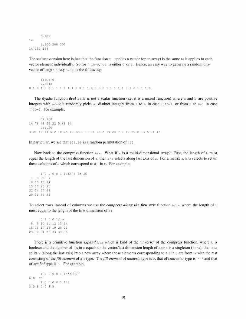
Now back to the compress function b/a. What if a is a multi-dimensional array? First, the length of b must
equal the length of the last dimension of a; then b/a selects along last axis of a. For a matrix a, b/a selects to retain
those columns of a which correspond to a 1 in b. For example,
1 0 1 0 0 1 1/m<-5 7#!35
1 3 6 7
8 10 13 14
15 17 20 21
22 24 27 28
29 31 34 35
To select rows instead of columns we use the compress along the first axis function b/.a where the length of b
must equal to the length of the first dimension of a:
0 1 1 0 1/.m
8 9 10 11 12 13 14
15 16 17 18 19 20 21
29 30 31 32 33 34 35
There is a primitive function expand b\a which is kind of the ‘inverse’ of the compress function, where b is
boolean and the number of 1‘s in b equals to the vector/last dimension length of a or a is a singleton (1=^a); then b\a
splits a (along the last axis) into a new array where those elements corresponding to a 1 in b are from a with the rest
consisting of the fill-element of a‘s type. The fill-element of numeric type is 0, that of character type is ’ ‘ and that
of symbol type is `. For example,
1 0 1 0 0 1 1\'ABCD'
A B CD
1 0 1 0 0 1 1\8
8 0 8 0 0 8 8

20
1 0 1 0 0 1 1\`ab `c `d1 `eeh
`ab ` `c ` ` `d1 `eeh
And the companion function expand along the first axis b\.a is similarly defined on a multi-dimensional array a as
in the case of compress.
There is a dyadic primitive function membership a?b which for each element in a it asks whether the element
belongs to b and gives 1 if yes, 0 if no. Hence, the result of a?b is boolean and the shape a?b of is the shape of a.
For example,
5?'A'
0
w
njvfl
fnlup
afbpw
12ABC
w?'abcdefghijk1'
0 1 0 1 0
1 0 0 0 0
1 1 1 0 0
1 0 0 0 0
A finite numeric (character/symbolic) set can obviously be represented as a vector sv in ELI provided that each
element of s appears only once in sv; and if a predicate P applicable to elements of the set can be expressed as an
ELI boolean expression PB, then the set
{x | P(x), x� s}
can be expressed in ELI as
(PB(sv))/sv
For example, if sv is !10 and P is ‘x is an even number’ then PB is 0=2|sv:
(0=2|sv)/sv<-!10
2 4 6 8 10
and the complement of that set is (~PB(sv))/sv:
(~0=2|sv)/sv<-!10
1 3 5 7 9
In general, if a is a vector representing another set, then the complement of sv with respect to a is
(~sv?a)/sv
For two ‘sets’ a and b, the intersection of the two is the following:
(a?b)/a
The difference between a set and a vector is that in a set the elements are unique while a vector can contain
duplicate elements. There is a monadic primitive function unique =a which eliminates duplicates in vector a:

21
='njvflfnlupafbpw12ABC'
njvflupabw12ABC
=2 1 3 1 2 5 4
2 1 3 5 4
For two vectors a and b, a,b is just a vector with b glued to a. Hence, the union of two sets represented by a and b is
=a,b
The monadic form of ? is the where function: for a boolean vector b, ?b gives the positions of 1s in b depending
on []IO:
?0 1 0 1 0 1 0 0 0 0 1 1 1 0 0 1 0 0 0 0
2 4 6 11 12 13 16
[]IO<-0
?0 1 0 1 0 1 0 0 0 0 1 1 1 0 0 1 0 0 0 0
1 3 5 10 11 12 15
While the dyadic function a?v indicates which elements of a belongs to v, for a vector v, the dyadic function
index of v!a gives more information: the position (index) of each element in a first appears in v and for elements of
a which is not in v the corresponding result is 1+#v (or #v if a[]IO=0) indicating the element is out of bound of v.
The shape of v!a is the shape of a and we must have v and a of the same type. For example
'abcdefghijklmnopqrstuvwxyz'!'i like to see you'
9 27 12 9 11 5 27 20 15 27 19 5 5 27 25 15 21
a<-5 7#!35
a
1 2 3 4 5 6 7
8 9 10 11 12 13 14
15 16 17 18 19 20 21
22 23 24 25 26 27 28
29 30 31 32 33 34 35
#v<-2 3 5 7 11 13 17 19 23 29 31 37 39
13
v!a
14 1 2 14 3 14 4
14 14 14 5 14 6 14
14 14 7 14 8 14 14
14 9 14 14 14 14 14
10 14 11 14 14 14 14
1.6 Array Indexing, Indexed Assignment and taking Sections
We have already seen that elements of an array can be selected by the compress function. More conventionally,
elements of an array can be selected by their positions in an array, i.e. indexing as in any other high-level
programming languages. Indexing in ELI depends on []IO , the index origin, which we assume to be 1 here unless
specified otherwise.
n<-55 47 77 93 31 96 7 58 45 16
n[1]
55
n[3]
77
n[10]
16

22
[]IO<-0
n[1]
47
n[3]
93
n[10]
index error
n[10]
^
We can see that for []IO=0 it is just like in C, and if the index is out of bound it would result in an index error.
More importantly, an array can be indexed by a vector: as long as each element of that vector is within index bound,
n[!3]
55 47 77
n[5+!5] (or n[6 7 8 9 10])
96 7 58 45 16
and one can scramble order of indexing, have repetition in indexes and even a change of shape in indexing set:
n[5 2 3 1]
31 47 77 55
n[6 6 5]
96 96 31
m<-3 4#!10
m
1 2 3 4
5 6 7 8
9 10 1 2
n[m]
55 47 77 93
31 96 7 58
45 16 55 47
For a vector n and an array I we always have
#n[I] �� #I
where each element of I must be an integer from !#n.
For a matrix (or an array of higher dimension), ordinary scalar indexing as well as vector indexing are all allowed
with indexing coordinates to each dimension separated by a ‘;’:
c
ABCD
EFGH
IJKL
c[2;4]
H
c[2 3;4]
HL
c[2 3;1 4]
EH
IL
c[;4]
DHL
c[1 2;]
ABCD
EFGH

23
where an empty expression before or after a ‘;’ indicates that all elements in the corresponding axis would be taken.
In general, if a is an k-dimensional array, then an index expression
I �� I1;I2;…;Ik
is legal for a provided that each Ij is either empty or is an integer expression whose value (or value of its elements
in case of an array) lies within !(#a)[j]. Each Ij is called a component of the index expression I. For such an
index expression, the shape of a[I] is the Cartesian product of shapes of Ij‘s. For example,
a<-2 3 4#!24
a
1 2 3 4
5 6 7 8
9 10 11 12
13 14 15 16
17 18 19 20
21 22 23 24
a[1;2 3;1 2 4]
5 6 8
9 10 12
a[;1 3 2;2 4]
2 4
10 12
6 8
14 16
22 24
18 20
What happen if one of the element in Ij is not in !(#a)[j]? Simple, the system will respond with a message
index error
and execution stops.
We have already introduced assignment
Av<-expre
informally in section 1.2, where Av is the name of an ELI variable and expre is any valid ELI expression, i.e. its
evaluation (to be explained in detail in the next chapter) must result in a well-defined value. The expression can
involve several function applications or can simply be a literal value or another variable which already has a value.
In particular, if we want to assign a value such as !0 to several variables B, C, D, E we can write in one line
B<-C<-D<-E<-!0
The result of the assignment is that the variable on the left of <-will have the value of the expression on the right of
<-. Unlike typed languages like FORTRAN, C or Java, there is no restrictions what so ever on the variable or the
expression of either sides of <-, i.e. any legal expression can be assigned to any variable at any time. In FORTRAN
or C, a variable must be declared implicitly or explicitly to be of certain type, say, integer, floating-point or character,
and only expressions of corresponding type can be assigned to a particular variable. In ELI, a variable can change

24
from a floating-point matrix to a character vector or scalar symbol at any time (though it is not a good programming
practice to change the type of a variable at a whim). This saves user the hassle of variable declaration. More
importantly, it let you program with variables whose dimensions or sizes can change during program execution.
Besides the simple assignment we discussed above, ELI provides another kind of assignment, called indexed
assignment of the following form:
Arv[index_expre]<-expres
where Arv must be a variable whose current value is an array, index_expre is an index expression of Arv as we have
discussed earlier on indexing an array (a vector, matrix or multi-dimensional array). Unlike in the case of simple
assignment, there are restrictions on expres: First, must be of the same storage-type as that of Arv, i.e. they must be
both numeric, or both character or both symbolic. Second, expres must be either a scalar or of the same shape as
that of index_expre. The effect of the indexed assignment is the replacement of the values of the elements of the
array selected by index_expre as in indexing by the corresponding elements of expres (in case there are repeat
elements in index_expre then the later ones in expres overwrite earlier ones). If expres is a scalar, then every
selected element of the array is replaced by that scalar. For example,
av<-!12
av[2 3]<-12 13
av
1 12 13 4 5 6 7 8 9 10 11 12
av[2*!6]<-0
av
1 0 13 0 5 0 7 0 9 0 11 0
a<-2 3 4#!24
a[1;2 3;3 4]<-2 2#!4
a
1 2 3 4
5 6 1 2
9 10 3 4
13 14 15 16
17 18 19 20
21 22 23 24
a[2;;1 3 4]<-1
a
1 2 3 4
5 6 1 2
9 10 3 4
1 14 1 1
1 18 1 1
1 22 1 1
Combined with the monadic function where ?, we have a very convenient way to replace certain elements in a
vector such as ’A’ by ’a’ in ch and all negative numbers in w by 0:
ch
A book named 'ABC'
ch[?ch='A']<-'a'
ch
a book named 'aBC'
w
_1.5 2 3.1 _0.3 10 9 _3

25
w[?w<0]<-0
w
0 2 3.1 0 10 9 0
We note that indexed assignment is the only kind of assignment which allows expressions other than a variable
name appear on the left side of <- in ELI.
Many times, one would like to take some segment of a vector v (section of an array) and there is a dyadic take
function ^. to do just that: for a vector v the function n^.v, where n must be an integer, can be illustrated by the
following examples:
3^.1 2 3 4 5 6 7
1 2 3
_3^.1 2 3 4 5 6 7
5 6 7
9^.1 2 3 4 5 6 7
1 2 3 4 5 6 7 0 0
i.e. for n>0 (resp. n<0 ) n^.v takes the first (resp. last) elements of v, and if |n|>#v, additional slots are filled by a
typical element of the type of v. If the right argument of take is a matrix a, the left argument must be a vector n2 of
length 2; n2[1] indicates the number of rows of a to take along the first axis and n2[2] indicates the number of
colunms to take along the second axis (and this principle is extended to multi-dimensional right argument, i.e. the
length of the left argument vector must equal to the rank of the right argument). For example,
A
abcd
efgh
ijkl
abcd
2 3^.A
abc
efg
_1 2^.A
ab
We note the take of a vector always ends in a vector. Hence, for a vector a there is a subtle difference between
a[1], which is a scalar since its index, 1, is a scalar, the first element of a, and 1^.a which is a one element vector
made out of the first element of (##a[1] is 0 but ##1^.a is 1). In fact, for a vector a, we have a monadic primitive
function first ^.a for a[1].
a<-11 3.2 9 10
a[1]
11
^.a
11
##^.a
0
1^.a
11
##1^.a
1
There is a dyadic primitive function called drop (n!.a) which is the opposite of take: it drops the first, if n>0
(resp. last, if n<0) elements of a and returns the rest, assuming a is a vector:

26
1!.a
3.2 9 10
3!.a
10
_2!.a
11 3.2
5!.a
##5!.a
1
#5!.a
0
0!.a
11 3.2 9 10
#0^.a
0
We note that if n>=#a the result is an empty vector. We also see that 0 drop of a returns a while 0 take of a is an
empty vector. This rule for drop on vectors can easily be extended to multi-dimensional right arguments similar as
in the case of the take function, i.e. the first element of left argument applies to the first axis of the right argument
and so on. For example, for the matrix A appeared previously,
1 2!.A
gh
kl
_1 0!.A
abcd
efgh
1.7 Array Transformations
ELI provides many primitive mixed functions to transform whole arrays or make a new array out of one or two
argument arrays. In fact, we have already seen such examples in the take and drop functions in the previous section
that make new arrays out of sections of an argument array. We shall start with the monadic ravel function ,a, which
turns its right argument a into a vector consisting of the same elements as that of the original array in raveled order:
m
1 2 3 4
5 6 7 8
9 10 11 12
,m
1 2 3 4 5 6 7 8 9 10 11 12
If a is a vector then ,a �� a (invariant). If a is a scalar, however, the result is an one element vector.
a<-2
b<-,a
b
2
#b
1
#a
(* an empty vector *)

27
The dyadic function a,b is called catenate which ‘glues’ its two arguments a and b. For a which is either a scalar
of a vector and b which is of similar type as that of a, we have
'A','CE'
ACE
a<-1 3 5
b<-2 4 6 8
a,b
1 3 5 2 4 6 8
s<-3#`abc
s1<-`dkb
s,s1
`abc `abc `abc `dkb
For more general case, a,b (called a catenate b ) concatenates two arrays along the last axis. For example, with
m above and n below, are two matrices with equal length first axis, we have:
n
0 0 0
0 0 0
0 0 0
m,n
1 2 3 4 0 0 0
5 6 7 8 0 0 0
9 10 11 12 0 0 0
n,m
0 0 0 1 2 3 4
0 0 0 5 6 7 8
0 0 0 9 10 11 12
One of the argument to catenate can be a scalar or a vector while the other is a matrix (in the 2nd
case, the length of
the vector must equal to the length of the 1st dimension of the array). For example,
m,30
1 2 3 4 30
5 6 7 8 30
9 10 11 12 30
m,3 33 99
1 2 3 4 3
5 6 7 8 33
9 10 11 12 99
What about catenate, i.e. glue, two arrays along the first axis? Indeed, ELI has a function catenate along the
first axis, a,.b, to do so with similar requirements on its arguments as in the case of a,b:
n1
0 0 0 0
0 0 0 0
m,.n1
1 2 3 4
5 6 7 8
9 10 11 12
0 0 0 0
0 0 0 0
m,.30
1 2 3 4
5 6 7 8
9 10 11 12

28
30 30 30 30
m,.3 33 66 99
1 2 3 4
5 6 7 8
9 10 11 12
3 33 66 99
We note that a,.b can also be specified as a,[1]b (for []IO=1 or a,[0]b for []IO=0). This [1]is called an axis
specification and can be applied to an axis other than the first or the last (see [4]).
For two arrays a and b of the same shape, we can specify a fractional number f in the axis specification to get a
new array a,[f]b which joins the two argument arrays along a new axis whose relative position is specified by f.
This function is called laminate. For example,
c
1 2 3 4 5
d
0 0 0 0 0
c,[0.5]d
1 2 3 4 5
0 0 0 0 0
c,[1.5]d
1 0
2 0
3 0
4 0
5 0
We see that if f<1 (the first dimension here since c is a vector) then the newly created axis is the 1st axis; if f>1
(the last axis) then the newly created axis is the last axis.
If we want to generate a vector v of n integers start from s and p apart, we set []IO<-0 and write
v<-s+p*!n
Now, suppose we like to list a short table of a regular sequence of 10 temperatures in Celsius starting at -5 and 3
degrees apart with their corresponding Fahrenheit temperatures, we do the following:
[]IO<-0
_5+3*!10
_5 _2 1 4 7 10 13 16 19 22
c<-_5+3*!10
32+1.8*c<-_5+3*!10
23 28.4 33.8 39.2 44.6 50 55.4 60.8 66.2 71.6
c,[0.5]32+1.8*c<-_5+3*!10
_5 23
_2 28.4
1 33.8
4 39.2
7 44.6
10 50
13 55.4
16 60.8
19 66.2
22 71.6

29
In comparison with the C program to do conversion in [11], we see that C relies on loops to do computation on
array elements whereas in ELI arrays are first class citizens manipulated by language primitives operating on arrays
to eliminate the need of looping in many cases. This is what we mean by programming with arrays.
The monadic function reverse $a reverses the elements of an array a along its last axis, or any other axis
specified by an axis operator $[f]a. For example ([]IO=0),
$!5
4 3 2 1 0
$m
4 3 2 1
8 7 6 5
12 11 10 9
$[0]m
9 10 11 12
5 6 7 8
1 2 3 4
In particular, for the temperature conversion code above, we may prefer to list from high temperatures to lower ones:
c,[0.5]32+1.8*c<-$_5+3*!10
22 71.6
19 66.2
16 60.8
13 55.4
10 50
7 44.6
4 39.2
1 33.8
_2 28.4
_5 23
We note that reverse of a along the first axis can simply be written as $.a.
The dyadic function rotate n$a rotates the elements in a with the amount specified by n, which must be integral
and its length must equal to the rank of a, in such a way that a positive integer indicates the amount of elements
moved from left to right (or top to bottom in case of rotating along first axis) and a negative integer indicates a
rotation in reverse direction.
v
1 2 3 4 5
2$v
3 4 5 1 2
_1$v
5 1 2 3 4
For a multi-dimensional array a as the right argument of n$a (resp. n$.a), the shape of n is required to be
#n �� _1!.#a (resp. #n �� 1!.#a)
i.e. drops the part of shape of a representing the dimension of the axis it is rotating about; and each element in n
indicates how the corresponding row (resp. column) in a is to be rotated. For example,
A
abcd

30
efgh
ijkl
1 2 3$A
bcda
ghef
lijk
2 0 1 3$.A
ibgd
afkh
ejcl
For a multi-dimensional array a such as a matrix, the left argument n to the rotate function n$a can be a scalar. In
this case n is expanded to (##a)#n, i.e. the rows or columns of a will be rotated the same amount n. For example,
1$A
bcda
fghe
jkli
_1$A
dabc
hefg
lijk
1$.A
efgh
ijkl
abcd
_1$.A
ijkl
abcd
efgh
The monadic function transpose &.a reverses the order of axis of a. In case of a matrix, it just exchanges the first
axis with the last axis of the argument. For A above, we have
&.A
aei
bfj
cgk
dhl
m2<-2 3 4#!24
&.m2
1 13
2 14
3 15
4 16
5 17
6 18
7 19
8 20
9 21
10 22
11 23
12 24

31
The dyadic function general transpose n&.a where n is a vector of length equal to the rank of a with elements
coming from shape vector of a. We will not go further into details but just note that 1 1&.a is taking the diagonal of
a:
1 1&.A
afk
1.8 Operators and Derived Functions
Besides an abundance of primitive functions (in fact, we have not presented all primitive functions in ELI yet),
what makes APL/ELI so powerful are the operators it provides. An operator in ELI applies to one or two primitive
scalar functions to produce a new function, called a derived function. We have already encountered the reduction
operator / applied to the add function +, +/, earlier in sect. 1.6, and we can also regard the axis modification [x] of
compression and expansion as an operator on the compress and expand functions (these are not scalar functions).
The regular operators are the following:
The reduction operator denoted by / takes a left function argument f, which must be a dyadic scalar function, to
produce a new monadic derived function f/. For a vector v whose elements are v1,v2,… vn
f/v �� v1fv2f… fvn
We have already seen earlier that +/ is the summation function, and it is easy to see that */ is the product function.
Other useful derived functions from reduction are the maximum ~./ and minimum _./ functions:
~./3.2 4 8 0.2 9
9
_./3.2 4 8 0.2 9
0.2
The result of f/A for a vector A is always a scalar; see [4] for cases of an empty vector V (+/V is 0 and */V is 1).
In general, we have
#f/A �� _1!.#A (#f/.A �� 1!.#A)
In other words, f/A always results in an array with a rank 1 less than the rank of A. For an array A, the reduction
always applies along the last axis. To do reduction along the first axis, we use the operator, reduce along 1st axis
f/.A . For example,
m
1 2 3 4
5 6 7 8
9 10 11 12
+/m
10 26 42
+/.m
15 18 21 24
The scan operator denoted by \ also applies to a left argument function f, which must be a dyadic primitive
scalar function, to produce a monadic derived function f\. If v is v1,v2,… vn, a vector of n elements then the k-th
element of f\v is f/wk, where wk is the vector v1,v2,… vk (i.e. k^.v). For example,

32
a
1 2 3 4 5
+\a
1 3 6 10 15
*\a
1 2 6 24 120
^\1 1 0 1 0
1 1 0 0 0
&\0 0 1 0 0
0 0 1 1 1
We see that +\ is the partial sum function and *\ is the partial product function. When and-scan ^\ applies to a
boolean vector b it produces a new boolean vector whose elements becomes 0 once a 0 element is encountered in b.
For the or-scan &\, it produces a boolean vector whose element starts to be 1 once a 1 is encountered.
Let c be the coefficient vector of a polynomial, and we assume []IO=0, i.e. c represents the following polynomial
of degree n:
c[0]+c[1]x+c[2]x*x+…+c[n]xn
If we want to evaluate this polynomial at point p, we do
+/c*1,*\(_1+#c)#p
We note that the expression to the right of scan is a vector of n(=(#c)-1) p‘s, and the scan results in a vector whose
successive elements are increasing powers of p.
The application of f\ to general arrays is similar to that of f/, i.e. along the last axis; and there is a companion
operator f\., scan along the first axis. For example,
+\m
1 3 6 10
5 11 18 26
9 19 30 42
+\.m
1 2 3 4
6 8 10 12
15 18 21 24
The outer product operator .: applies to a right argument function f which must be a dyadic scalar function
and produces a dyadic derived function .:f. For vectors v and w, v.:f w is a matrix M whose individual element is
defined as follows:
M[i;j] �� v[i]f w[j]
For example,
a0<-1 2 3
a
1 2 3 4 5
a0.:*a
1 2 3 4 5
2 4 6 8 10
3 6 9 12 15
a0.:<a

33
0 1 1 1 1
0 0 1 1 1
0 0 0 1 1
In general, for arrays A and B, A.:f B is a Cartesian product of A and B, and we have
#A.:f B �� (#A),#B
i.e. the shape of the result of applying the derived function of an outer product to two arguments is the catenation of
the shapes of the argument arrays, and each element of the result is from a pairwise application of the argument
function f to corresponding elements in the argument arrays.
Outer product is often used to construct a table for a range of various input values. For example, if one deposits
1000 dollars at 3% annual interest rate, after one year one would have 1000*1.03 and 1000*1.03*1.03 in two
years. During ten years period, the money grows as
1000*1.03*.1 2 3 4 5 6 7 8 9 10
To see how 1000 dollars will grow under 3%, 5% and 8% of annual interests in 10 years, we do
1000 *1.03 1.05 1.08 .:*. !10
1030 1060.9 1092.727 1125.5088 1159.2741 1194.0523 1229.8739 1266.7701 1304.7732 1343.9164
1050 1102.5 1157.625 1215.5063 1276.2816 1340.0956 1407.1004 1477.4554 1551.3282 1628.8946
1080 1166.4 1259.712 1360.489 1469.3281 1586.8743 1713.8243 1850.9302 1999.0046 2158.925
The inner product operator denoted by ‘:’ takes two dyadic primitive scalar function arguments f and g to
produce a dyadic derived function f:g, which for two vectors v and w of equal length is defined as follows:
v f:g w �� f/v g w
For example,
v<-2 5 1 4
w<-1 9 6 7
v~.:+w //ELI parser scans from left to right, so it is interpreted as v(~.):+w
14
v+:~.w
24
The (derived function of) inner product f:g extends to arrays M and N along the last axis M of and the first axis of N.
Hence, we must have (_1^.#M)=1^.#N, and the shape of the result of the application of the derived function is
#M f:g N �� (_1!.#M),1!.#N
For example,
m
1 2 3 4
5 6 7 8
9 10 11 12
n
1 2 3
4 5 6
m+:*n

34
length error
m+:*n
^
n+:*m
38 44 50 56
83 98 113 128
n*:+m
168 312 504 750
750 1056 1428 1872
We can see that for two numeric matrices n and m, n+:*m is the familiar matrix product of n and m. But other inner
products are also useful. Suppose T is a 10 by 8 name-table and n1 is a name (of 8 characters padded with blanks):
T
Anthony
Backus
Cocke
Codd
Donath
Eastman
Fagin
Gabriel
Harrison
Lucus
n1<-'Cocke '
T^:=n1
0 0 1 0 0 0 0 0 0 0
?T^:=n1
3
That means n1 is the third name in the table as only the 3rd
row of T matches every character in n1.
1.9 Lists and Operations on Lists
A fundamental data structure in ELI which is not in classical APL [9] is the list: a list is a group of items, each of
which can be a scalar, an array, or another list, separated by ‘;’:
l<-(1 2;`abc;'vb')
l
<1 2
<`abc
<vb
We see that items in a list, unlike that in an array, can be of different types or even of different structures. Hence, in
ELI we use lists to organize non-homogeneous data. What can we do on lists? First, we can apply shape function #
(or count ^) to a list to get the number of items in it:
#l
3
reshape does not work for lists, but a special case of reshape works for allocating a list of n empty items (denoted
by the underline symbol _) or get a 0 item list:
#Ln<-3#_ 3

35
l0<-0#_
#l0
0
A list can be indexed like a vector. Most importantly, a list L can be assigned to a group of variables all at once,
where the number of variables is equal to #L. A list can be entered with items containing expressions or another list:
l[1 3]
<1 2
<vb
(n;s;c)<-l
n
1 2
s
`abc
c
vb
a<-2 3 4
(a+1;$'avc';;!10)
<3 4 5
<cva
<
<1 2 3 4 5 6 7 8 9 10
A scalar s or an array a is not a list, to make an one item list of it, we employ the monadic primitive function
enclose <.:
#L<-<.2 4#!12
1
L
<1 2 3 4
5 6 7 8
take, first, drop and catenate work on lists the same way as they work on vectors (see [4] sect.2.1). In particular,
for a one-item list L1 first ^.L1 serves as disclose of L1, i.e. it turns L1 back into a scalar or an array:
^.L
1 2 3 4
5 6 7 8 #^.L
2 4
The each operator ” operates on lists, or a scalars/array and a list. For a monadic function f, and a list L, f”L is
evaluated by applying f to each component item L[j] of L to result in a list Z of the same structure as that of L, i.e.
#f”L is of the same length #L and each element of Z[j] is fL[j] which must be well-defined for all j.
#"l
<2
<
<2
3#"l
<1 2 1
<`abc `abc `abc
<vbv
ln<-(!5;!10)
ln
<1 2 3 4 5

36
<1 2 3 4 5 6 7 8 9 10
+/"ln
<15
<55
We see that unlike in operators for functions on arrays in the previous section, the argument f to the each operator is
not restricted to scalar primitive functions; it can be a mixed function, a derived function or even a defined function
(see next section).
For a dyadic function g, the derived function g” is also a dyadic function: for two lists L and R, g” is defined as
(L g” R)[i] �� L[i] g R[i]
for each i in !#L, where we must have(#L)=#R, and as in monadic case, g can be a mixed function, derived
function or a defined function, but for each i, L[i] g R[i] must be well-defined; either L or R can be a scalar or a
one-item list by replacing L[i](resp. R[i]) with L(resp. R) in the formula above. For example,
(1;2;3)$"(!5;!8;!10)
<2 3 4 5 1
<3 4 5 6 7 8 1 2
<4 5 6 7 8 9 10 1 2 3
1+"(!5;!8;!10)
<2 3 4 5 6
<2 3 4 5 6 7 8 9
<2 3 4 5 6 7 8 9 10 11
(2 3;3 4)#"<.!10
<1 2 3
4 5 6
<1 2 3 4
5 6 7 8
9 10 1 2
Note that in the last example it is necessary to enclose !10 to make it a one-element list, otherwise, it will result in a
length error. See section 2.3 in [4] for more examples of each operator.
Suppose we have a linear algebra class and students taking the course are from three departments: mathematics,
computer science and engineering; and we enter the final test scores of students by departments as follows:
score<-(math;cs;eng)<-(70 85 72 88 69 96 58 100 75 60;87 77 64 50 92 80 73 96;84 73 66 97
54 79 62 81 70)
math
70 85 72 88 69 96 58 100 75 60
cs
87 77 64 50 92 80 73 96
eng
84 73 66 97 54 79 62 81 70
score
<70 85 72 88 69 96 58 100 75 60
<87 77 64 50 92 80 73 96
<84 73 66 97 54 79 62 81 70
First, we notice that the list notation allows us to assign multiple variables at once. Now we would like to count the
number of students from each department, the total score and the average score as well as the maximum/minimum
score for students from each department.
#"score
<10
<8
<9

37
+/"score
<773
<619
<666
(+/"score)%"#"score
<77.3
<77.375
<74
~./"score
<100
<96
<97
_./"score
<58
<50
<54
In fact, we can write a short function (see the following section 2.1) which gives the average of a numeric vector
{avg0:(+/x)%^x}
avg0
avg0 80 90 76
82
and apply each to it to get the same result
avg0"score
<77.3
<77.375
<74
What if we just want to count, calculate the total, average, maximum/minimum of the whole class? Easy, there is
a monadic function raze (,.) which turns a homogeneous list (i.e. the list elements are of the same type) into a vector,
and then we can simply apply appropriate functions to that vector:
,.score
70 85 72 88 69 96 58 100 75 60 87 77 64 50 92 80 73 96 84 73 66 97 54 79 62 81 70
#,.score
27
+/,.score
2058
avg0 ,.score
76.22222222
~./,.score
100
_./,.score
50
Now suppose the test scores of the whole linear algebra class was entered as a vector in a random fashion but an
accompanying vector of symbols indicates which department the student with that score comes from:
mscore<-88 66 64 92 96 85 84 81 87 54 70 77 80 72 96 62 100 73 75 70 60 58 79 69 50 73 97
dps
`math `eng `cs `cs `math `math `eng `eng `cs `eng `math `cs `cs `math `cs `eng `math `eng `math
`eng `math `math `eng `math `cs `cs `eng
Can we reconstruct a list of scores by departments to get a departmental view of the performance of students in the
linear algebra class? Indeed, it is quite simple to do so. First, there is primitive monadic function unique (=) in ELI
which when applying to a vector v will yield unique elements of v; so

38
=dps
`math `eng `cs
Second, there is primitive monadic function grouping (>.) in ELI which when applying to a vector v will yield a
list of length the number of unique elements in v and each item of that list consists of the indices of elements in v
equal to a particular elements in =v as follows
>.dps
<1 5 6 11 14 17 19 21 22 24
<2 7 8 10 16 18 20 23 27
<3 4 9 12 13 15 25 26
Third, for a vector v and a list I such that sub-elements of I are valid indices of v, then v[I] is a list of the same
structure as that of I with corresponding elements being the indexed elements of v; so
mscore[>.dps]
<88 96 85 70 72 100 75 60 58 69
<66 84 81 54 62 73 70 79 97
<64 92 87 77 80 96 50 73
Thus, we reconstructed test scores of the class according to the departments the students are from.
2. Defined Functions, Control Structures and Files
2.1 Defined Functions, Short-Form and Order of Evaluation
We have seen many examples of ELI expressions, now we would like to find a way to save these codes for reuse:
we put the code into a defined function by switching to the edit mode of ELI. The edit mode is triggered by a del-
symbol @. followed by a function name fn, or a function name together with formal parameter name(s):
@.fn
and end the edit mode by entering a matching @.. A parameter is a variable whose value is assigned at the time of
function call from that of an actual parameter; the rule to form a function name is the same as that for a variable
name (see sect. 1.2). Just like primitive functions, a defined function can be monadic or dyadic, i.e. take a right
argument only, or take a left argument as well as a right argument. However, a defined function can take no

39
argument and it is then called a niladic function. And unlike a primitive function which always gives a result, a
defined function can give a result or return no result. These distinctions of a defined function are all evident in the
first line (line [0]) of a defined function which is of the following form
function-header <;local-variable-list>
function-header must be one of the six forms below:
type valence have result no result niladic 0 R<-FN FN
monadic 1 R<-FN B FN B
dyadic 2 R<-A FN B A FN B
where valence is the number of arguments which the function takes, R is the name of the returned result, FN is the
name of the function, A is the name of the left argument and B is the name of the right argument (you can, of course,
give different names to each one of them). The arguments can also be arrays and lists, not just scalars. One can use
an explicit list notation on the right argument to effectively input more than 2 arguments. For example, after type
@.z<-a try (b;c)
then type two lines z<-a*b+c and @. in the function edit panel to get a defined function try. We then test it and
display its definition:
3 try (5;6)
33
{try}
---------try--------
[0] z<-a try (b;c)
[1] z<-a*b+c
--------------------
We note that use {fn} to display function fn only works after fn has been executed. To see a function text right
after it is defined, we can use the system function []CR which returns the character matrix of pure function text:
[]CR 'try'
z<-a try (b;c)
z<-a*b+c
The local-variable-list in the function header-line is optional; it is required only if you wish to localize a
group of variables. The list starts with a ‘;’, and variable names in the list are separated by ‘;’. If a variable named
V1 is localized in a function AF, then V1 must first be assigned a value in AF before it can be used in AF. The
parameter(s) and the result, if any, of a defined function are automatically localized. We just point out that unlike
in C where a variable is either local (to a procedure) or global, a variable in an ELI function fn can be local to some
function fn1 which calls fn directly or through a chain of calling functions. In other words, the scoping rule in ELI
is dynamic, not static as in PASCAL (see sect. 3.1 in [4] for a more detailed explanation of shading).
When a function
@.z<-a fn b;… …
…
@.

40
is called by v fn w, a gets the value of v and b gets the value of w before the code body of function fn starts to
execute. The parameter passing mechanism in ELI is by-value, i.e. values of v and w would not be changed when
the function fn returns no matter what happen to a and b during the execution of fn.
We remark that even though it looks like a defined function can take only two parameters, by using a list as the
right parameter we can actually pass in multiple parameters; for example, with a function head of the following form
@.z<-a fn (b1;b2;b3);…
we can pass 4 parameters.
From the previous chapter, we already have a good feel as how an ELI expression is evaluated. State more
formally: a line of ELI code L, also called a simple ELI statement, is a group of constants and variables interspersed
with primitive functions, derived functions and defined functions, and possibly with parentheses. We note here that
the assignment <- is also regarded as a primitive function. To evaluate L, one starts with the right most item r in L
which must be either a literal constant, a variable name or a niladic function name with a result, in case it is a ‘)‘ we
move to the left to evaluate the sub-line up to a matching ‘(’ to get a value. In case it is a variable name, ELI
fetches its value; in case of a function name, ELI executes that function to get a resulting value. Execution of L fails
if either variable value is missing of function runs into trouble; otherwise we have a value v. Either we reach the
end of L or we proceeds to the item l next to the left in L; l must be i) a primitive or derived function symbol pf or ii)
a defined function name fn. In case of i) and pf is ambivalent, we check to see whether there is an item on the left
of pf which will result in a value w and decides pf to be dyadic. This includes the case of a ‘)’ for which we call
evaluate recursively to the sub-line up to a matching ‘(’ to get a value w. We either get a new value w pf v, or pf v
if there is no item to the left of pf. In case of a defined function fn then whether we proceed to get w fn v or fn v
is determined by the valence of fn. In any case we replace v by the new value, and either we continue to evaluate
leftward or we reach the end of evaluation of L. If at any step, we run into problem such as a missing value (value
error) or mismatched arguments (length error or doamin error), the execution stops with an error message. A
successful evaluation of L always results in a value V. For example,
ln2blk[n]<-fblkx<-fblkx+newblk<-newblk&nx<-n?lx
is an ELI statement. The rule of equal precedence among primitive functions is almost necessary in view of the
abundance of primitive functions in ELI. This simple rule also enables a natural concatenation of many operations
into one line, thus contributes significantly to the succinctness of ELI programs. Parsimony of symbols is a form of
economy in the cleric aspect of preparing a program which also reduces the chance of committing trivial error.
Quite often, one would like to write a simple function of one or a few short lines. ELI provides a short-form
function definition facility for that convenience as follows
{fnam: …}
where fnam is the name of a function, and either z or the last expression is the result of the function while x is the
right argument, and y is the left argument if present; all other variables are assumed to be local. All statements must
be a simple or if statement (see sect. 2.3); two statements can be separated by ‘;’ in one line. Moreover, statements
in short-form definition cannot access any global variable other than system variables. In addition, comment line(s)
must be outside of the function body {..}, and a short-form definition of a defined function can be entered in
execution mode of ELI, i.e. interactively. For example
//average of a numeric vector

41
{avg: (+/x)%^x}
avg //response to the definition
avg 4 5 0.8 10 4.7
4.9
The average of a vector is the sum divided by the number of elements in it. The reason we used ^ instead of # is
that x could be one number only, i.e. a scalar.
Let us consider the problem of finding the greatest common divisor of two integers x and y. The function gcd2 in
short-form below solves that problem:
{gcd2:_1^.(0=(a|x)+a|y)/a<-!x_.y}
gcd2
18 gcd2 8
2
6 gcd2 27
3
This is a rather naive algorithm: take the smaller of the two numbers, generate a vector a from 1 up to that number
and select those elements of a which can divide evenly into (using modulo function |) both x and y, and take the last
one from the resulting vector. While this function is quick to code in ELI and avoids the complication of if-then-else
and iterations, for very large x and y, the function is quite inefficient as it incurs unnecessary computations. But it
has one advantage, i.e. it can turn into a vector form effortlessly: instead of finding the greatest common divisor of
two numbers, suppose we want to find the greatest common divisor of x which is a vector of positive integers. We
have
{gcd:_1^.(^/0=a.:|x)/a<-!_./x}
gcd
gcd 18 8
2
gcd 45 15 20
5
gcd 9 21 60 18 24
3
The algorithm is the same as in gcd2. We just used derived functions on a vector and a matrix produced by an outer
product. This example illustrates the essence of array-oriented programming in ELI, i.e. utilizing array operations
whenever possible, instead of picking scalar elements and doing sequential iterations. While ELI is not strictly a
functional language in the sense of Haskell, its programming style is quite functional, i.e. for many programming
tasks, an ELI program needs very few, or no state variables to accomplish a job; it is as mathematical as a program
can be formulated. Nevertheless, as we pointed out earlier, an array-oriented solution of a problem may be wasteful
and problematic for very large input parameters, it has another potential advantage: an array-oriented program in
ELI is easier to be parallelized by a compiler for multi-core machines without user’s involvement (see [6]). This
could be quite attractive as we know that to parallelize a program is typically a painstaking and time consuming task.
2.2 One-liner Functions
2.2.1 number conversion and lexicographic ordering
Given a sequence x of hexadecimal digits, how do we convert x into its binary representation? Let us first introduce
the primitive function encode r<.c; for scalar c and vector r (called the radix vector), it produces a result of shape
#r which encodes c in the numerical system of r. For example,

42
24 60 60<.3670
1 1 10
means that 3670 minutes is one day one hour and ten minutes; and
2 2 2 2<.12
1 1 0 0
is the binary representation of 12. The encode function extends to array a in such a way that the result is of rank
1+##a and each column vector along the first axis is the result of applying r to that element of a. For example,
2 2 2 2<.12 9 5
1 1 0
1 0 1
0 0 0
0 1 1
For a string of hexadecimal digits c we first convert it into a vector of numbers by querying the relative positions of
the digits in the standard character list of hexadecimal digits (we must set []IO to 0 first) using the index of function:
[]IO<-0
'0123456789ABCDEF'!'C95'
12 9 5
We then apply encode to it, but the binary form of each digit is in a column. So we flip the resulting matrix and then
ravel it. Hence, the function is the following
{x2b:[]IO<-0; ,&.(4#2)<.'0123456789ABCDEF'!x}
x2b
x2b '89ABCD'
1 0 0 0 1 0 0 1 1 0 1 0 1 0 1 1 1 1 0 0 1 1 0 1
We note that there is an inverse function to encode, i.e. the decode function r>.c (sect. 1.9 in Primer [4]). For
example,
24 60 60>.1 1 10
3670
2 2 2 2>.1 1 0 0 12
2>.1 1 0 0 12
We see that the difference is that if the left operand is a scalar then it will automatically expand to be a vector of the
length of the right operand.
Let TABLE be a 8 by n array of names, i.e. each TABLE[i;] is a string of 8 characters of English alphabets and digits
with trailing blanks. We want to sort TABLE into lexicographical order. There are two monadic sort functions
grade up < and grade down > in ELI. For a numerical vector v, <v (resp. >v) gives the indices of elements of v in
a non-decreasing (resp. non-increasing) order rearrangement. For example (we assume here []IO=0):
v<-10?.100 //pick 10 distinct numbers randomly from 0..99
v
5 52 67 0 38 6 41 68 58 93

43
<v
3 0 5 4 6 1 8 2 7 9
v[<v]
0 5 6 38 41 52 58 67 68 93
The grade up and grade down functions in ELI also apply to character vectors with respect to lexicographical order.
For example,
c<-'awgnkn09'
<c
6 7 0 2 4 3 5 1
c[<c]
09agknnw
To solve our problem, we first note that the grade up function only applies to a vector argument. The following
function extends < along the last axis, i.e. it gives indices of sorted elements in each row:
{mgrdu: s#,.<"(w<-_1^.s<-#x)||,x}
What the function does first is to turn the input matrix into a list of rows using the partition function ||(sect. 2.1 [4]).
It then apply the each operator " to the grade up function < on each row and put the resulting list of rows back into a
matrix using the raze function ,. (sect. 2.1 [4]). To illustrate,
m<-8 5#40?.100
m
82 12 1 68 86
62 73 72 99 88
23 30 35 51 59
84 41 26 53 46
28 17 15 57 80
3 49 95 74 55
89 21 71 13 9
27 0 2 70 93
mgrdu m
2 1 3 0 4
0 2 1 4 3
0 1 2 3 4
2 1 4 3 0
2 1 0 3 4
0 1 4 3 2
4 3 1 2 0
1 2 0 3 4
However, to get the relative size (weight) of each row in m we need to apply mgrdu again:
mgrdu mgrdu m
3 1 0 2 4
0 2 1 4 3
0 1 2 3 4
4 1 0 3 2
2 1 0 3 4
0 1 4 3 2
4 2 3 1 0
2 0 1 3 4
Now suppose that above is from a grade up of a flipped 8 by n name table, to put that in a lexicographical order

44
where the order of the first character dominates the second and so on the numeric weights of the names is calculated
by the decode of the numbers representing the weight from ordering at each row. Hence, we have
8>.mgrdu mgrdu m
4203553 2658906 6635784 1160915 9308292
Therefore, the solution to our problem is the following function:
{lexord:[]IO<-0;x[<8>.mgrdu mgrdu &.x;]} table
abUni95w
jklmnboa
bUni95wj
klmnboab
Uni95wjk lexord table Uni95wjk
abUni95w
bUni95wj
jklmnboa
klmnboab
2.2.2 a queuing network model
There is a PASCAL program in chapter 6, Performance Analysis, Desrochers [7], which implements the Boyse
and Warn closed queuing network model. We shall only compute up to the average CPU queuing length lq. The
reader who wants to go further will find that the whole 4-page program there can be put in ‘one-line’ ELI code once
lq is calculated. By ‘one-line’ we mean that it may not be physically fit, or desirable, to be squeezed into one line
but there is no transfer of control when we break it into several lines. The inputs to the model are
c number of CPUs
k multiprogramming level, c<k
e_o mean service time for each I/O processor
e_s mean service time fot each CPU
What to be computed are
p_o_0 probability of 0 jobs in the system
p_o_h probability of h jobs in the system
ratio(j) ratio of p_o_n/ p_o_0 for j:=1..k
lq average CPU queue length
The PASCAL program segment to compute the ratio(j) is
if j<=c then
ratio:=factorial(k)/(factorial(j)*factorial(k-j)*power(e_s/e_o,j)
else
ratio:=factorial(j)/(factorial(c)*power(c,j-c))
*factorial(k)/(factorial(j)*factorial(k-j)*power(e_s/e_o,j)
To put this in one-line ELI, we have to remove the use of if-then-else which would have been easy except for the
fact that for j>c there is an extra factor multiplying into it. Let jl<-!k (i.e. 1...k). The tentative code is
ratio<-temp*((|.k)%(|.jl)*|.k-jl)*(e_s%e_0)*.jl

45
where temp is a vector of length k with first c elements =1, and elements from c+1 to k equal to
factorial(j)/(factorial(c)*power(c,j-c))
Let jtl<-c+!k-c. Then jtl is a vector of length k-c ranges from c+1 to k, and the tail section of temp above is
jtvl<-(|.jtl)%(|.c)*c*.jtl-c
Therefore, temp is
temp<-(c#1),jtvl
and r=ratio is
r<-((c#1),(|.c+jt)%(|.c)*c*.jt<-!k-c)*((|.k)%(|.jl)*|.k-jl)*(e_s%e_o)*.jl
p_o_0 is
p_o_0 = 1/(1+sum)
where sum is the summation of ratio over all j. In ELI, we have
p_o_0<-1%1++/r
Note that in ELI we use the ’,’ primitive to glue different formulae to replace a loop with if-then-else in PASCAL
and use the reduction operator to avoid a loop in summation. According to [7] the probability of h jobs in system
and the average CPU queue length is computed in PASCAL as follows
lq:=0 for i:=1 to k do
begin p_o_h:=ratio(j)*p_o_0;
if i>c then lq:=lq+((i-c)*p_o_h)
end;
So in ELI with p_o_h now stands for a vector from j=1 to k,
p_o_h<-r*p_o_0
and lq is the summation of a vector qv of length (k-c) whose right factor is a portion of p_o_h from i=c+1 to k:
qv<-(!k-c)*(c-k)!.p_o_h
Now remember that the take function (-j)!.v will take elements from rear of v. To put it all together, the function
BW_qmodel below computes the average CPU queue length z= lq in the Boyes and Warn closed queuing network
model where o= e_o , s= e_s and p= p_o_h:
@.z<-c BW_qmodel (k;o;s)
z<-+/jt*(c-k)!.p<-r*1%1++/r<-((c#1),(|.c+jt)%(|.c)*c*.jt<-!k-c)*((|.k)%(|.jl)*jl)*(o%s)*.jl<-!k
@.

46
2.3 Control Structures
So far we have only given examples of straight-line codes. To write code involves alternatives or iterations
classical APL [9] provides branching and ELI provides that as well; and that only appears in defined function
definition. The simplest branch statement is
->0
that means function return. Another is
->msg
where msg is a character string and activation of this statement will output msg and then stop ELI execution. This
statement is used when a program runs into exceptions. For example, if a piece of code runs into
->’name not found’
then ELI will emit the error message ’name not found’ and stop execution. A more general branch statement is of
the form
->(boolexpr)/L
where boolexpr is an expression of boolean value and L is a label as statement in ELI can have a label like
L: expre
if boolexpr is 0 execution will continue to the next statement else the execution will branch to the statement with
label L (see [4] for more forms of branching).
However, ELI provides control structures similar to those in C. In ELI a simple statement is either a line of code
resulting in an expression as we described in 2.1 or a branch statement. A statement is either a statement or a group
of (multi-line) statements bracketed by a pair of {}. Other than simple statement, ELI has the following statements
if-statement: if (boolean expression) statement [[else if (bool expression)]” else statement
case-statement: case (case expression) {case-lists [else statement]}
where case-list : v1[,v2..vn]: statement
for-statement: for (idxv:for-forment) statement
where for-forment: strv;endv[;step] or idxlist
while-statement: while (boolean expression) statement
In a case statement, case expression must result in a discrete scalar type, i.e. an integer, a character or a symbol.
We shall see their usage through various examples later; but we first give a recoding of the 31-line APL function
OPERATION in Digital System Implementation [1] p.138 which specifies the set of System/360 operations. inst is a
boolean vector representing an instruction where bits 4-7 is the portion for op-code with comments after line(s)
being the op-code name; od1 is the first operand, od2 the second operand and rl1 the result, all in bits. TWOC is the
2-complement interpretation function and ARCHDIV is the divider architecture. Note the result of multiplication is a
64-bits vector putting into two pieces of 32-bits code, and in division a double precision dividend dd is used which is

47
comprised of two operands od2 and od3. An interested reader can compare the following code with that in [1] and
see clearly that the case statement in ELI makes the code more intuitive and close to the original intention.
@.OPERATION
case (2>.inst[4 5 6 7]) {
//data handling
0: rl1<-(32#2)<.|TWCO od2 //POS
1: rl1<-(32#2)<.-|TWCO od2 //NEG
3: rl1<-(32#2)<.-TWCO od2 //COMP
2,8: rl1<-od2 //LOAD
//logic
4: rl1<-od1^od2 //AND
6: rl1<-od1&od2 //OR
7: rl1<-od1~=od2 //XOR
//arithmetic
10,14:rl1<-(32#2)<.(2>.od1)+2>.od2 //ADD
5,9,11,15:rl1<-(32#2)<.(2>.od1)-2>.od2 //SUB
12:{pd<-(64#2)<.(TWCO od1)*TWCO od2 //MPY
rl1<-32^.pd
rl2<-32!.pd}
13:{dr<-od1 //DIV
dd<-od2,od3
ARCHDIV
rl1<-qt
rl2<-rm}
}
@.
2.4 Recursion
2.4.1 sorting
Recursion is a powerful programming technique to solve some seemingly complicated problems in a systematic
way. It is the main programming paradigm in LISP. In APL/ELI, we usually try to find non-recursive solutions in
terms of array operations first before we try recursion. Nevertheless, recursion is an integral part of APL/ELI. In
general, recursion applies to data which are irregular, or not array like. But recursion can still be applied to vectors
and arrays to yield some elegant solutions. Let us start with a sorting example.
We already know from sect. 1.5 that there is a lexicographical ordering among characters. We shall define an
ordering gre_eq (>=) between two character strings s1 and s2 as follows where si[1] is the first character of si:
if s1[1]>s2[1] then s1>= s2 is 1
if s1[1]<s2[1] then s1>= s2 is 0
if s1[1]=s2[1] then compare 1!.s1 with 1!s2
empty string < non-empty string
Hence, our comparison function is as follows:
@.z<-le gre_eq ri
if (0=^le)
if (0=^ri) z<-1 else z<-0
else if (0=^ri) z<-1
else if ((l1<-1^.le)>r1<-1^.ri) z<-1
else if (l1=r1) z<-(1!.le) gre_eq 1!.ri
else z<-0
@.
'bab' gre_eq 'b'

48
1
'bab' gre_eq 'cb'
0
'b' gre_eq 'b0'
0
The problem we want to solve is how to sort a vector of symbols such as
v<-`abc `wx `a0 `c123 `cd
where the order of each pair of symbols is determined by the order of their character string representations as we just
defined above. Hence, the steps are
1. turn +.v into a list sl of character strings representing the symbols
2. apply the quicksort algorithm to the list sl
3. put the sorted list of strings back into a vector of symbols
To do 1, we observe that
+.v
abc wx a0 c123 cd
We see that it is a vector consists of characters denoting symbols in v separated by a blank but with ‘`’ taking out.
We append a blank in front of it and then get a boolean vector indicating blank or non-blank. We then use the
monadic function partition count || to get a count of each string starting with a blank; from there we apply the
count function to the slightly modified v in dyadic partition || to get a list of strings each with a blank affixed in
front of a character string representing a symbol in v and we then apply 1!.” to drop that blank.
' '=' ',+.v
1 0 0 0 1 0 0 1 0 0 1 0 0 0 0 1 0 0
||' '=' ',+.v
4 3 3 5 3
(||' '=v1)||v1<-' ',+.v
< abc
< wx
< a0
< c123
< cd
1!."(||' '=v1)||v1<-' ',+.v
<abc
<wx
<a0
<c123
<cd
The quicksort algorithm is invented by Tony Hoare. The basic idea is very simple. It takes one element x from a
list L and divide L into two piles: pile1 consists of elements less than x and pile2 consists of those greater than or
equal to x; it then applies the same procedure recursively to pile1 and pile2. Hence, our code is (where x is just the
first element of L)
@.z<-sortsyms v;v1
z<-!.,.’`’,” quicksort 1!."(||' '=v1)||v1<-' ',+.v
@.
@.z<-quicksort ls;b

49
if (1>=#ls) {z<-ls
->0}
z<-(quicksort (~b)/ls),quicksort (b<-ls gre_eq” 1^.ls)/ls
@.
b is the result of gre_eq comparison of each element in ls with ls[1] and b/ls is the compression of ls by b. We
note that for a list z of character strings, ’`’,”z affix a ’`’to each element in z, and the raze function z,. just ravels
a list of homogeneous data back into a vector. For example,
,.(2 5 7;8 10;9; 22 100 _3 1)
2 5 7 8 10 9 22 100 _3 1
And we already mentioned in sect. 1.3 that the execute function !.c will turn certain character vector c into a
vector of symbols.
However, the code thus presented has a fatal error which is not easy to find out by testing which by nature can
only run a finite number of times. To prove the correctness of a program P, we must first prove the P will end, i.e.
it will terminate. There is no question that a straight line ELI code (segment) with only primitive functions and
derived functions will terminate. Hence, sortsyms will terminate if and only if quicksort will. For a recursive
function rf to terminate the recursive calls inside rf must be applied to data of smaller pieces, for otherwise the
chain of recursive calls will be endless. Here we find the problem: it is entirely possible that ls[1] is the ‘smallest’
of ls thus b is all 1 and b/ls is ls again. Once we realize the problem, to fix the bug is quite simple:
@.z<-quicksort ls;b;w
if (1>=#ls) {z<-ls;->0}
z<-(quicksort (~b)/w),l1,quicksort (b<-w greeq” l1<-1^.ls)/w<-1!.ls
@.
What we did is taking the first element out of the dividing process and put it in the middle of two piles, one with
smaller elements and one with larger or equal elements. Now the arguments to the recursive calls must have length
less than that of ls because w itself is of length one less than that of ls.
We make a comment on the effort to prove program correctness here. As Dijkstra pointed out that no amount of
testing can vouch for the correctness of a program. Hence, the goal of proving program correctness is certainly
noble and recently there are substantial successes in its application to the area of OS and hardware implementations.
Nevertheless, for most good size programs, especially C programs with pointers, this remains a formidable task and
only of academic interest. What APL/ELI brings to the table is that by subsume many if-then-else and loops into
high-level primitives and put substantial portion of code into one-line segments it reduces the logical complexity of
a program considerably as we have seen in the formulation of the function sortsyms above. Therefore, succinctness
of ELI code is not just a matter of esthetic taste but brings clarity which reduces error and helps program reasoning.
There is another slightly different way to sort a list of symbols without using list. We turn the vector of symbols
into a matrix of rows of character strings of equal length and apply the quicksort algorithm by taking the first row
and compare it with the rows in the rest of the matrix. Once the character matrix is sorted, we turn it back into a
vector of symbols by first affixing ‘`’ in front of it and then applying the execute function !..
((^v),1)#v
`abc
`wx
`a0
`c123
`cd

50
+.((^v),1)#v
abc
wx
a0
c123
cd
@.z<-quicksort2 ls;b;w;i;r;s;l1
if (1>=r<-^.s<-#ls) {z<-ls;->0}
w<-1 0!.ls; l1<-ls[[]IO;]
b<-(r-1)#0
for (i:1;r-1) b[i]<-w[i;] gre_eq l1
z<-(quicksort2 (~b)/.w),.l1,.quicksort2 b/.w
@.
@.z<-sortsyms2 v;v1
z<-!.,'`',quicksort2 m<-+.((^v),1)#v
@.
sortsyms2 v
`a0 `abc `c123 `cd `wx
2.4.2 tower of Honoi
The Tower of Honai is a game with three poles A, B, C and a set of n disks fit onto a pole, say A, by means of a
hole cut through the center of each disc. The discs are of increasing size from top to bottom. The game is to move
all discs from A to C one disc at a time, but a larger disc should never put on top of a smaller one. B can be used as
an intermediate resting place for transient discs. The problem looks complicated until we assume that that a sub-
problem has already been solved. Suppose we can find a way to move the first n-1 discs from pole A to pole B. We
only need to move the n-th disc from A to C, and then move the n-1 discs from B to C. Let
k discmove poles
be a function call to move k discs from poles[1] to poles[3] using poles[2] as an intermediate place (poles is
represented by three characters A,B,C). The program is
@.n discmove poles
if (n=1) {
[)<-'move the first disc from '
[)<-poles[1]
[)<-' to '
[]<-poles[3]
->0}
(n-1) discmove poles[1 3 2]
[)<-'move '
[)<-n
[)<-'-th disc from '
[)<-poles[1]
[)<-' to '
[]<-poles[3]
(n-1) discmove poles[2 1 3]
@.
We note here both []<-expr (called quad output) and [)<-expre (called bare output) are to output the right side
expr in ELI. The difference is that for the bare output the next output will follow where it left off, i.e. no line-end

51
character will be at the end of this output. The termination condition for the discmove function is clear as the
recursive call is with left argument n-1. We take a sample run of three discs:
3 discmove 'ABC'
move the first disc from A to C
move 2-th disc from A to B
move the first disc from C to B
move 3-th disc from A to C
move the first disc from B to A
move 2-th disc from B to C
move the first disc from A to C
2.4.3 determinant
For a square matrix m, we would like to find its determinant det m recursively. First, if m is of rank 1, i.e. m is
of the form [a] then is a. Next if m is of rank 2, i.e. m is of the form
|a b|
|c d|
then det m is ad-bc. For a general m, if we can rearrange m into a form with its first row all 0 except the first a11,
and let us denote the sub-matrix of m formed by rows and columns from second on m1. Then det m is a11*det m1.
Of course, the rearrangement needs to leave the determinant invariant. The code is the following:
@.z<-det m;n;p;i //det of a matrix nxn to nxn.
i<-[]IO
case (n<-1^.#m) {
1: z<-m[i;i]
2: z<-(m[i;i]*m[i+1;i+1])-m[i;i+1]*m[i+1;i]
3: z<-+/(*/.0 1 2$m)-*/.2 1 0$m
else {
if (^/m[i;]=z<-0) ->0
if (0=m[i;i]) {m[;p,i]<-m[;i,p<-(0=m[i;])!0]
m<--m
}
m<-m-(m[;i]*%z<-m[i;i]).:*0,m[i;1!.!n]
z<-z*det 0 1!.1 0!.m
}
}
@.
Here for the case rank=3, we employed a direct formula to calculate the result. The reader can check a linear
algebra book to verify that the code indeed implement the formula where for example,
m
1 2 3
4 5 6
7 8 9
2 1 0$m
3 1 2
5 6 4
7 8 9
0 1 2$m
1 2 3
5 6 4

52
9 7 8
the rotations rotate each row of m a different amount and */. is column-wise product while +/ is the sum. In the
else part covering the general case, we first check whether the first column is all 0 and in that case the result is 0. In
case the left upper corner element is 0, p<-(0=m[i;])!0 find the first non-zero element in the first row m[i;] and
then exchange the corresponding columns by m[;p,i]<-m[;i,p]. Since this exchange will change the sign of det m
we do m<--m. The next line reduce all other elements in the first row to 0, and the last line makes the recursive call
to the sub-matrix of m formed by dropping the first row and first column of m. For a test run,
m
4 _7 27 7 22
28 40 9 3 23
_6 35 12 29 14
2 8 _1 15 36
16 6 _5 38 10
det m
_5965161
2.5 Script Files
A user can prepare his/her ELI code in an ordinary text file of extension txt or esf. A script file can contain
function definitions in full format or in short-form. For a function sf defined in short-form any function f called
inside sf must be defined before the definition of sf. A script file can also contain definitions of variables and
executable statements. To input a variable in a file, one write a head line first
&vnam type rank shape
where vnam is the name of the variable, type is a character indicating the type of the variable (‘B’ for boolean, ‘I’
for integer , ‘E’for floating-point, ‘C’ for character, ‘S’ for symbol etc. see [4] for others), rank and shape are the
rank and shape of vnam. Starting from the next line is the raveled value of vnam where elements are separated by a
blank space except in the case of character variable for which blanks are significant, but not required in case of
symbol type. A variable input is ended by a line with a single ‘&’. For example for the variable
m3
1 2 3
4 5 6
7 8 9
the script input is
&m3 I 2 3 3
1 2 3 4 5 6 7 8 9
&
If we have large input from a source other than hand prepared text, we only need to insert head line and end line to
make it into a legitimate input to ELI.
ELI variables and functions can also output to a text file from an ELI session or a loaded ELI workspace by the
command
)out file1 fn1 fn2 a b

53
This would result in a script file file1.esf containing functions fn1 fn2 and variables a b. If there is no name
following the file name file1 then everything in the session or workspace will be output to the file file1.
ELI system comes with a script standard.esf which contains many useful pre-defined functions. Hence,
)fcopy standard
will copy in the script file, then a group of frequently used utility functions are available. See section 4.4 in [4] for
examples.

54
3. Array Implementation of Data Structures
3.1 Emulation of PASCAL Data Structures in ELI
3.1.1 a small database for a company
Suppose we want to build a database of personnel information for a company C. The information for each
employee of this company is represented as a record in the PASCAL programming language as follows:
type employee= record name: array [0..7] of char;
phone: array [0..11] of char;
division: array [0..7] of char;
manager: ↑ employee;
subordinates: ↑ employeelist; salary: integer;
sex: (male, female);
birthdate: array [0..2] of integer;
status: (fulltime, parttime, fired, retired);
yearhired: integer;
yearterminated: integer;
end;
type employeelist= record
first: ↑ employee; next: ↑ employeelist; end;
where indicates that manager and first are fields of pointer type points to record of type employee. The type is just
PASCAL’s way of implementing a linked list (see Wirth [14] sec.4.2), and the field
subordinates: ↑ employeelist;
represents the list of employees directly reporting this employee in case he is a manager. We encounter three im-
mediate problems when try to implement this database in a way similar to the PASCAL case:
1. there is no record structure or struct in ELI,
2. there is no pointer type in ELI,
3. ELI does not have the build-in procedure new(p) of PASCAL to dynamically create an item of the type the
pointer p points to.
Before we set to solve these problems, let us reflect on what we want: a data structure where an employee’s
record can be created for new hires, status change due to promotion, demotion, firing or retiring can be easily
updated, and the hierarchy of the company should be evident in the database. Moreover, we would like to have
various queries about the company and its divisions answered quickly.
First we observe that the database can be implemented in PASCAL as
array [0..totalnumber] of employee;
where totalnumber is the total number of employees in the company. But it has one problem in PASCAL: to add a
new employee we have to declare another array of length totalnumber+1. In ELI, there is no array declaration and

55
an array A can be appended by a new item simply by:
A<-A,newitem
Since a record in PASCAL is in essence a collection of fields, we can use a collection of arrays in ELI to emulate an
array of records in PASCAL (in this chapter, we use []IO=0):
ename<-(totaln,8)#’ ‘ ephone<-(totaln,12)#’ ‘ ediv<-(totaln,8)#’ ‘
emangr<-totaln#_1
esubos<-totaln#_1
esubon<-totaln#0
esalary<-totaln#0
esex<-totaln#’ ‘
ebdate<-(totaln,3)#0
estatus<-totaln#’ ‘
ehire<-totaln#0
eterm<-totaln#0
where totaln is the total number of employees. Then each record in the original PASCAL implementation is
represented by a collection of values of arrays at a specific index, say i. For example, the array ename is a totaln
by 8 matrix of characters, and
ename[i;] tramble
represents the (truncated or padded with blanks to 8 characters) name of an employee in the i-th slot of the database;
and
ephone[i;]
914-456-7688
is the phone number of that employee. The array
emangr
which corresponds to a field of pointer type in PASCAL is initialized to _1 which stands for the nil value in
PASCAL; and
emangr[i;]
is an index j between 0 and totaln which represents the manager of tramble(i.e. if tramble has a manager) named
ename[j;]
If tramble is the CEO of the company, then he has no manager and j=_1. Note that there are two arrays esubos,
esubon correspond to the field
subordinates: ↑ employeelist;
in PASCAL. This is because we decide to use a numeric array
56
employeelist
of indexes to represent the corresponding linked list in PASCAL such that esubos[i] points to a starting location in
employeelist of a list of indexes representing employees who directly report to trimble, and esubon[i] is the
length of that list. Hence, the list of indexes of employees reporting to a manager if index i is
employeelist[esubos[i]+!esubon[i]]
and the name of these employees can be printed by
ename[employeelist[esubos[i]+!esubon[i]];]
While ELI has symbol type, here we simply use two characters ‘m’ and ‘f’ to represent (male, female) and ‘f’, ‘p’,
‘x’, ‘r’ to represent the values of the corresponding field of status. To add a new employee
name: Johnson
phone: 914-456-8366
division: Reseach
..
status: fulltime
yearhired: 2003
we do
ename<-ename,.8^.’Johnson’ ephone<-ephone,.’914-456-8366’
ediv<-ediv,.’Research’
..
estatus<-estatus,.’f’
eyhire<-eyhire,.2003
and the old totaln becomes the employee identification number in this database while
totaln<-totaln+1
At this point we want to introduce the concept of cost of a computation informally. Each ELI primitive
operation is implemented by a group of machine operations (codes), and some are more costly than others in terms
of execution time or storage requirement. For example, the operation
a<-a,newpart
is far more costly than the operation
i<-i+1
regardless of whether newpart is a scalar (i.e. a single item) or a large array. Not getting into the fact that ELI is
interpreted and there is an interpreter-overhead associated with the execution of any ELI expression, this can be
intuitively explained as follows. While the second expression only involves adding i by 1, which can basically be
accomplished by one machine instruction, the first expression involves the creation of a new array in the computer
memory, copying the values of the old array to the new array area and then copying the value of newpart next to it.
The ability to device a more efficient program with the same functionality is what separates an experienced ELI/
APL programmer from a beginner. All one-line examples in the last chapter can be implemented with loops in the
C/ PASCAL fashion. The reason an experienced APL programmer is likely to choose an array-oriented solution is

57
mostly due to the fact that a one-liner executes far faster than a loopy solution under an interpreter system,
especially when computer memory is tiny. And this is how historically an array-oriented programming style
developed in the APL community. However, an unforeseen advantage is that an array-oriented program is more
amenable to automatic parallelization under an advanced compiler (see Ching and Zheng [6]).
Back to the programming task at hand, we realize that by adding a new item to each component array in our
database when adding a new employee is a bad design if the company is likely to add new employees fairly
frequently. An alternative design would be to allocate a collection of arrays to a size a bit larger than the expected
size of the company and keep tracking what it the next employee identification number which is the same as the
total number of employees ever recorded in the database since we choose to use []IO=0. Hence, we have
@.initialize nxtempn<-nxtsen<-0
maxnem<-1000+incnemp<-1000
ephone<-(maxnem,12)#’ ‘
ediv<-(maxnem,8)#’ ‘
emangr<-maxnem#_1
esubos<-maxnem#_1
esubon<-maxnem#0
esex<-maxnem#’ ‘
ebdate<-(maxnem,3)#0
estatus<-maxnem#’ ‘
eyhire<-maxnem#0
eyterm<-maxnem#0
employeelist<-maxnem#_1
@.
to initialize the database. To insert a new employee record, we first check whether our table (i.e. the collection of
arrays is large enough to contain the new record. In case space is already exhausted then we increase the size of the
table by a fixed, but large chuck. The function is
@.z<-inc
if (maxnem>=1+z<-nxtempn) ->0
else { //increase the table by a chunk of size incnem
ename<-ename,.(incnem,8)#’ ‘
ephone<-ephone,.(incnem,12)#’ ‘
ediv<-ediv,.(incnem,8)#’ ‘
emangr<-emangr,incnem#_1
esubos<-esubos,incnem#_1
esubon<-esubon,incnem#0
esex<-esex,incnem#’ ‘
ebdate<-ebdate,.(incnem,3)#0
estatus<-estatus,incnem#’ ‘
eyhire<-eyhire,incnem#0
eyterm<-eyterm,incnem#0}
@.
Under this new organization, the previous segment of code to enter information for new employee Johnson becomes
ename[i<-inc;]<-8^.’Johnson’
ephone[i;]<-’914-456-8366’
ediv[i;]<-’Research’
..
estatus[i]<-’f’
eyhire[i]<-2003

58
3.1.2 implementation of linked lists in ELI
We want to study our implementation of a linked list using two component fields esubos, esubon and a storage
array employeelst. For the sake of simplicity, let us assume for the moment that all employees have unique names
which are at most eight characters long. Suppose the new employee Johnson is reporting to a manager named Brook
and one of his subordinate named Peters has just left. Recall from section 1.8 (T tnow is ename[!nxtempn;], the
matrix containing names of all employees ever employed by company C) that the expression assigned to z in the
following function
@.z<-find nam
if (nxtempn<=z<-(ename[!nxtempn;]^:=8^.nam)!1)
[]<-‘No employee named ‘,nam,’ in this company’
@.
returns the identification number of an employee with name nam, and when z=nxtempn means no match of the name
nam is found. Hence, first we do
emangr[i]<-j<-find ‘Brook’
To list all employees directly report to a manager named mnam, we have
@.manager_g mnam
[]<-enames[employeelst(esj<-esubos[j])+!esubon[j]]
@.
But we also need to update the field of subordinates for Brook. A simplistic approach would be to find where
Peters‘s identification number is located in employeelst and replace it by Johnson‘s id-number:
employeelst[employeelst!find ‘Peters’]<-i
However, as we will explain later, the id-number of Peters may appear in multiple instances in employeelst.
Therefore, a correct way to do updating is searching Peters‘s id-number thru the sublist of subordinates of manager
with id-number j:
slist<-employeelst[(esj<-esubos[j])+!esubon[j]]
and replace accordingly:
employeelst[esj+slist!find ‘Peters’]<-i
Now in case Peters left company, or started reporting to another manager, without any replacement, we must
adjust
esubon[j]<-newsen<-esubon[j]-1
More than that we must adjust the list slist above to eliminate the id-number of Peters from the list everywhere it
appears, and reassign to the storage array jemployeelst as follows:
employeelst[esj+!newsen]<-(slist~=find ‘Peters’)/slist

59
We note that the last id-number in slist is still in employeelst but becomes inaccessible because esubon[j] is 1
less than previously. This is why an id-number may appear more than once in employeelst due to such updating.
Next, suppose Johnson is simply a new hire, not a replacement. So his manager just has one more employee
reporting to him/her:
esubon[j]<-newsen<-esubon[j]+1
But we cannot just append the slist in employeelst by the id-number i because that slot may well be occupied
by the id-number of an employee who reports to another manager. We need a fresh segment in employeelst to
store the newly expanded list slist representing employees reporting to Brook. And to do that we need another
function similar to inc:
@.z<-inx n if (maxnem>=nxtsen<-n+z<-nxtsen) ->0
else // increase the list by a chuck of size incnemp
employeelst<- employeelst,incnemp#_1
@.
This function takes an argument n because we anticipate situations where a manager may increase the number of
subordinates by more than one. inx returns the first index of a size n segment in employeelst which is not
occupied as we use nxtsen to keep track of where new segment can start. Anyway, back to our case of adding
Johnson, we have
employeelst[(inx 1)+!newsen]<-slist,i
We realize that this use of pointer-vector and length-vector combination with one store-away array for
implementing a group of lists has serious draw-back: any time a particular list grows, a fresh storage-area will be
needed and a copy operation is required. An alternative approach is to use a imaxsen by 2 matrix
employeelink<-(maxsen,2)#_1
so that for a manager with id-number j
employeelink[jsx<-esubos[j];0]
points to (i.e. it is the id-number of) the first employee reporting to that manager and if
employeelink[jsx;1]
is not _1 then it points to a row in employeelink where the next employee (i.e. his id-number) reporting to the same
manager is located:
employeelink[employeelink[jsx;1];0]
is the id-number of that next employee. This chain of linked list of employees reporting to manager Brook ends at a
slot sx with
employeelink[sx;1]=_1

60
We still use nxtsen to keep track the next unused slot in employeelink, but we no longer need the component field
esubon to keep track of the length of a list. This implementation of a linked list is structurally similar to the
PASCAL’s type definition of type employeelist.
The function inx is now changed to
@.z<-inx1 if (maxnem>=nxtsen<-n+z<-nxtsen) ->0
else // increase the list by a chuck of size incnemp
employeelink<- employeelink,.(incnem,2)#_1
@.
To list all employees directly report to a manager named mnam, we have
@.manager_g mnam if (_1=sx<-esubos[find mnan]) {[]<-‘No one report to ‘,mnam;->0}
[]<-‘The following people report to ‘,mnam
while (_1~=sx) {
[]<-ename[employeelink[sx;0]
sx<- employeelink[sx;1]}
@.
To add an employee enam to the list of employees reporting to a manager named mnam we do
@.enam add_togp mnam
i<-find enam
if (_1=sx<-esubos[j<-find mnan])
employeelink[esubos[j]<-lx<-inx1;0]<-i
else {
while (_1~=sx) sx<-employeelink[sx;1]
employeelink[employeelink[sx;1]<-inx1;0]
}
@.
To delete an employee named enam from the list of people reporting to a manager named mnam, we do
@.enam drop_fmgp mnam
if (_1=sx<-esubos[find mnan]) {[]<-‘No one report to ‘,mnam;->0}
else if (_1=employeelink[sx;1]){
esubos[j]<-_1 // only one employee reporting to mnam
->0}
else {
i<-find enam
sx0<-sx
while (_1~=sx) {
if (found<-i=employeelink[sx;0]) break
sx<- employeelink[sx;1]
}
if (~found) []<-‘No one named ‘,enam,’ reported to ‘,mnam,’.’
else if (sx=sx0) esubos[j]<- employeelink[sx;1]
else employeelink[sx0;1]<- employeelink[sx;1]
}
@.
So we see that the program to list all employees reporting to a manager or to eliminate an employee from such a list
is more involved now, but we avoid copying a whole list of reporting employees when adding a new employee to

61
the corresponding list. Another possible alternative is to introduce a new component field esubom to reserve a
segment of length
esubom[find newmangrnm]
in employeelst when someone named newmangrnm is made a manager, and inX is called only when an addition to a
group of new subordinates will make the number of employees reporting to that manager larger than the prescribed
segment length. We will leave the detail of implementation to readers as an exercise.
3.1.3 implementation of queries to a database
The reason people want to implement databases about some organizations or certain areas of inquiry is that we
can efficiently find information related to that organization or area by making queries to the database of concern.
There are generally three kinds of queries: individual, global and departmental. An individual query is about one
person in the organization. For example, to find the phone number of an employee named nam
@.phone nam;i if (nxtempn<=i<-find nam)->’No employee named’,nam
else {
[)<-nam,’: ‘
[]<-ephone[i]
}
@.
phone ‘Johnson’
Johnson: 914-456-8366
Global queries are about the whole organization. For example, to find the number of full and part time employees,
we have
currentemployees<-+/(flst=’p’)&’f’=flst<-status[!nxtempn]
And the total amount of salaries which the company pays is
totalsa<-+/((flst=’p’)&’f’=flst<-status[!nxtempn]/nxtempn^.esalary
Note that there only nxtempn entries in the database which have been ever used, but the list also contains the last
salaries of former employees, i.e. those retired or fired. So we first have to set up a boolean mask to select entries of
full-time and part-time employees using the field status and then add them up.
Not all global queries result in a single number. For example, the following function will list all employees who
are paid more than twice of the average salary together with their salaries.
@.twicepay totalsa<-+/(mask<-(flst=’p’)&’f’=flst<-status[alst<-!nxtempn])/cursal<-nxtempn^.esalary
lst<-(esalary[curlst]>2*totalsa%+/mask)/curlst<-mask/alst
[]<-ename[lst;],+.((#lst),1)#esalary[lst]
@.
curlst is the list of id-numbers of current employees, and +/mask is the total number of current employees. Hence,
totalsa%+/mask is the average salary, and lst is the list of id-numbers of employees whose salary is more than
twice the average. Recall from Chapter 1.6 that the format function +. turns numeric data into their character

62
representations. But applying +. to esalary[lst] directly will result in a vector of characters while we want it to
be a matrix of characters (digits) such that each row is the salary of the employee with the same id-number.
Therefore, we apply a reshape to turn it into a lst by 1 matrix before applying +. to it. A simple illustration is the
following:
a<-132 756 459 533 219 48 679 680 935 384
+.a
132 756 459 533 219 48 679 680 935 384
a1<-10 1#a
a1
132
756
459
533
219
48
679
680
935
384
a1c<-+.a1
a1c
132
756
459
533
219
48
679
680
935
384
Let us write a related function: to list all employees (and their salaries) whose salaries are in the top 10% of all
employees. First we note that we cannot simply look for a number and select ones whose salary is over that
threshold; for this will not necessarily give us the top 10% of the employees. For our task, we literally have to sort
people in terms of their salaries and then take the top 10% to be listed:
@.top10pc
salist<-(mask<-(flst=’p’)&’f’=flst<-status[alst<-!nxtempn])/cursal<-nxtempn^.esalary
lst<-(_.0.1*+/mask)^.(curlst<-mask/!alst)[<salist]
[]<-ename[lst;],+.((#lst),1)#esalary[lst]
@.
We recall that curlst is the list of id-numbers of all currently active employees and <salist is the sorted list of
indexes from 0 to (+/mask)-1 so that salist[<salist] is a list of salaries in descending order. Hence,
curlst[<salist] is the list of id-numbers whose corresponding salaries are in descending order. Therefore, lst is
the top 10% list we want. We note a slight blemish here: there could be people with the same salary while one is
listed while the other is not. This is because we cut-off at the 10% boundary and a group of people with the same
amount of salary may have their id-numbers listed across that boundary.
A departmental query is about a division of a company. For example, the following function with parameter
dnam, the department name, lists all employees in that department with their names and phone numbers in
alphabetical order:

63
@.deptphone dnam
dlst<-(ediv[all]^:=8^.dnam)/all<-(estatus[all]?’fp’)/all<-!nxtempn
sdlst<-dlst[<27<.’ ABCDEFGHIJKLMNOPQRSTUVWXYZ’!enames[dlst;]] []<-ename[sdlst;],ephone[sdlst;]
@.
The first line gets all id-numbers of employees belong to the department named dnam. The second line sorts that list
into another list alphabetically as we explained in Chapter 2.4.3. We also remark that []<- in the last line as well as
in other examples is not really necessary. This is because the ELI interpreter will always display an expression if it
is not assigned to a variable. We used []<- merely to emphasize that an output is being carried out here.
Another example is that of calculating the ratio of managers to non-managers in a particular department named
dnam. The following function gives the percentage of managerial employees in a department.
@.z<-deptmratio dnam dlst<-ediv[all]^:=8^.dnam)/all<-(estatus[all]?’fp’)/all<-!nxtempn
z<-(+/_1~=esubos[dlst])%#dlst
@.
Note that for an id-number x, _1~=esubos[x] indicates that x is an id-number of a manager. We see that an
departmental query is really no different from a global query except the extra step to get the list dlst of id-numbers
in a given department.
3.2 Binary Trees
3.2.1 tree representation
Trees, especially binary trees, have been used extensively in programming to organize data into a structure on
which the operations of search, deletion and insertion can be implemented efficiently. One also would like to visit
every node of a tree in certain order. Trees are used in programming language implementation (parse trees),
artificial intelligence (game trees), data retrieval (binary search trees) and many other areas of application. A binary
tree is a tree whose node is either a leave node, i.e. a node without children, or has at most two child-nodes, a left-
son and/or a right son-node. Each node of a tree typically also contains a key which may represent the data item
stored at that node. The key can be a character string, a symbol, an integer or a bit-string of fixed length. Keys are
ordered and can be compared. Typically, the left sub-tree contains keys less than or equal to keys of the nodes on
the right sub-tree. The result of comparison of two keys, one given and one from a node encountered during a tree
visit guides an insertion or a search to go to left subtree, quit or go to right subtree. In PASCAL terminology, we
can declare a simple binary tree by
type tree = record
key: array[0..7] of char;
lson, rson: ↑tree;
end;
Following the approach of implementing such record structure in ELI, the function to initialize a tree structure is
@.inittree nxtndx<-0 maxndx<-1000+incndx<-1000
tkey<-(maxndx,8)#’ ‘
tlson<-trson<-maxndx#_1
alph<-’ ABCDEFGHIJKLMNOPQRSTUVWXYZ’
@.

64
A tree is represented by its root-node’s index. Initially, we have
root<-_1
And the function corresponds to new(tree) in PASCAL to create a new tree node is
@.z<-inct if (maxndx>=nxtndx<-1+z<-nxtndx) ->0
else {// increase the table by a chuck of size inctree
tkey<-tkey,.(inctree,8)#’ ‘
tlson<-tlson,inctree#_1
trson<-trson,inctree#_1
}
@.
Suppose the keys are to be ordered lexicographically and that characters appearing in keys are all in upper case
English alphabets. Then as explained in section 2.2.4 and the monadic signum function * mentioned in section 1.4
the following function
@.z<-lkey compare0 rkey z<-*(27<.alph!lkey)-27<.alph!rkey
@.
compares two keys lkey, rkey in lexicographical order and returns a 1 if lkey>rkey in that order, 0 if equal and _1
otherwise.
At this point we would like to discuss the concept of prototyping in a very high level programming language and
low-level programming. As readers who have experience of programming in other programming languages such as
FORTRAN, PASCAL or C/C++ can see that once one is fluent in APL/ELI, in general it is far faster to get a piece
of program coded in APL/ELI and get it running than in a sequential language where the natural unit of operation is
one cell and operations on an array are through loops over its elements. Therefore, historically APL was often used
as a prototyping language, i.e. used to build prototypes but not the final production code. By using a language like
APL to implement a prototype first has the advantage of checking out the basic algorithms and data structures in a
program design quickly. This is particularly attractive if the eventual implementation language is decided ahead of
time to be the assembly language of a particular machine or C. This is so because the APL interpreter provides a
high level and convenient debugging environment while most assembly language or C debuggers are of low-level
vista. Now most C/C++ comes with excellent IDE (interactive development environment). Nevertheless, debugging
in APL/ELI is still easier than debugging a corresponding program in C because it lets programmers to concentrate
on higher level abstractions in terms of primitives it provided (of course, there are many programming tasks which
require intimate interface with underlying operating system necessitate the use of a low level language such as C).
However, if we know a program such as compare0 is going to be re-implemented later in a lower level language we
would think twice. This is because we know that high level primitives like encode (<.) and iota (!) are not going to
be there in C or an assembler. An explicit effort not to use such primitives is what we refer to as low level
programming. A low level version of the comparison function is the following:
@.z<-lkey compare rkey for (x:!8)
case (*(alph!lkey[x])-alph!rkey[x]) {
_1: z<-1
->0
1: z<-1
->0

65
}
z<-0
@.
We note that the function compare compares one pair of characters at a time (similar to compare one bit at a time in
a radix sort where the keys are binary bit-strings), and yield a result as soon as the order can be determined where as
in compare0 a global calculation involving all characters in a key is always carried out. Clearly, the second
comparison function does less work. But due to interpreter overhead we mentioned earlier the second function may
execute slower than the first in most cases in APL/ELI, unless the code is compiled by an APL/ELI compiler.
However, for prototyping purpose, the second one is what we want as it avoids the use of two high level primitives.
3.2.2 tree operations
Suppose a tree already exists. Given a key key we would like to insert it into the tree or find the tree node (node
index) where the key have been placed. The algorithmic outline is
if the tree is nil then place the key at root else compare with the root node:
if key equals to the one at root then found else search the left subtree or the right subtree
and the ELI function is
@.z<-tree search key if(tree=_1) {z<-inct
tkey[z;]<-key}
else
case (*tkey[tree;] compare key) {
0: z<-tree
1: z<-tkey[tlson[tree];] search key
_1: z<-tkey[trson[tree];] search key
}
@.
Let nmat be a character matrix. Then the following function will build a tree out of nmat:
@.z<-buildtree nmat z<-search nmat[0;]
for(x: 1+!_1+1^.#nmat) search nmat[x;]
@.
To delete an item with key key from a tree, we use a recursive scheme similar to that in search. But we need to
do some cutting and reattachment when a node with the same key is found and removed. The basic algorithm is:
if the tree is nil then item not found
else compare with the root node:
if key equals to the root node then
if left subtree if nil then return right subtree
else
(find the right most descendent of left subtree,
detach it and put it in the place of the root)
else search the left subtree or the right subtree
Line 4 above is easy to understand (where [] represents the node to be deleted and ^ represents subtrees):
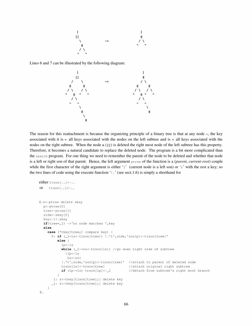
66
| | [] @
\ -> / \
@ ^ ^
/ \
^ ^
Lines 6 and 7 can be illustrated by the following diagram:
| | [] $
/ \ -> / \
@ @ @ @
/ \ / \ / \ / \
^ @ ^ ^ ^ @ ^ ^
/ \ / \
~ ~ ~ ~
\ \
@ @
\
$
The reason for this reattachment is because the organizing principle of a binary tree is that at any node n, the key
associated with it is > all keys associated with the nodes on the left subtree and is < all keys associated with the
nodes on the right subtree. When the node n ([]) is deleted the right most node of the left subtree has this property.
Therefore, it becomes a natural candidate to replace the deleted node. The program is a bit more complicated than
the search program. For one thing we need to remember the parent of the node to be deleted and whether that node
is a left or right son of that parent. Hence, the left argument ptree of the function is a (parent, current-root) couple
while the first character of the right argument is either ‘l’ (current node is a left son) or ‘r’ with the rest a key; so
the two lines of code using the execute function ‘!.’ (see sect.1.6) is simply a shorthand for
either tlson[..]<-..
or trson[..]<-..
@.z<-ptree delete skey p<-ptree[0]
tree<-ptree[1]
side<-skey[0]
key<-1!.skey
if(tree=_1) ->’no node matches ‘,key
else
case (*tkey[tree;] compare key) {
0: if (_1=ls<-tlson[tree]) !.’t’,side,’son[p]<-tlson[tree]’
else {
lp<-ls
while (_1~=rs<-trson[ls]) //go down right side of subtree
{lp<-ls
Ls<-rs}
!.’t’,side,’son[p]<-tlson[tree]’ //attach to parent of deleted node
trson[ls]<-trson[tree] //attach original right subtree
if (lp~=ls) trson[lp]<-_1 //detach from subtree’s right most branch
}
1: z<-tkey[tlson[tree];] delete key
_1: z<-tkey[trson[tree];] delete key
}
@.

67
The reason we want to organize data in a tree structure is for ease of searching, insertion and deletion. A tree
node n is an internal node if it has a left son or right son, i.e. tlson[n]~=_1 or trson[n]~=_1. A binary tree is
full if all its internal nodes have two sons. A tree is perfectly balanced if at any internal node, the difference in the
number of nodes in its two subtrees are less than or equal to 1. For example,
@ @ @ @
/ \ / \ / \ / \
@ @ @ @ @ @ @ @
/ \ / / \ / \ / / \
@ @ @ @ @ @ @ @ @ @
\
@
(1) (2) (3) (4)
Tree (1) is full but not perfectly balanced. Tree (2) is perfectly balanced but not full. Tree (3) is full and perfectly
balanced. Tree (4) is neither. The height of a tree is the maximum number of nodes from the root to a leaf node.
In a full and perfectly balanced tree of n nodes, approximately half of the nodes are leaf nodes and half are internal
nodes (see tree (3)). And the height of such a tree is log n. That means we only need to make log n comparisons
to locate an item instead of n. However, a tree can be such that each internal nodes has only one child. Then a
search in such a tree becomes linear such. For example, if nmat in the above function is the matrix t in section 2.1,
we then have such a skinny tree. The reason that this will result in linear tree is because t happens to be
lexicographically ordered to start with and the function buildtree builds the tree top-down. The following
function builds a perfectly balanced tree recursively for n number of nodes from bottom up, i.e. nodes of subtrees are
allocated before its root.
@.z<-buildtree2 n
if (n=0) z<-_1
else {
nr<-_1^.n-nl<-~.n%2
tkey[z<-inct]<-nmat[x<-x+1]
tlson[z]<-buildtree2 nl
trson[z]<-buildtree2 rl
}
@.
And to build a tree from as a set of keys for tree nodes, we do
x<-nxtndx buildtree2 n<-1^.#nmat
We note that the variable x in line 4 of the second tree building function is a global variable and need to receive a
value before the function can be called. Finally, we observe that although the tree built by buildtree2 is perfectly
balanced, it does not have the ordering property of a tree built by buildtree that for any node n, its key is greater
than any key (lexicographically) in its left subtree, and less than those on the right subtree. To build a tree which
has the ordering property and more balanced than simply using insertion function search requires more sophistica-
tion and we will not get into details here. Instead a reader can see Wirth [14] section 4.4.7.

68
3.2.3 tree transversals
A tree traversal is a way to visit nodes in a tree in certain order. In contrast, a search only aims at finding some
particular node in a tree. There are basically three ways to traverse a binary tree:
1. preoder: root, left subtree, right subtree
2. inorder: left subtree, root, right subtree
3. postorder: left subtree, right subtree, root
A / \
S R
/ \ \
D G H
For example, a preorder traversal of the tree above is
A S D G R H
An inorder traversal of the tree above is
D S G A R H
and a postorder traversal of the tree above is
D G S H R A
The (recursive) functions to do traversal are as follows where parameter tree is an index to arrays representing trees:
@.preorder tree
if (tree~=_1){
[]<-tkey[tree;]
preorder tlson[tree]
preorder trson[tree]
}
@.
@.inorder tree
if (tree~=_1){
inorder tlson[tree]
[]<-tkey[tree;]
inorder trson[tree]
}
@.
@.postorder tree
if (tree~=_1){
postorder tlson[tree]
postorder trson[tree]
[]<-tkey[tree;]
}
@.
However, many times we would like to have a non-recursive version of an algorithm. For example, if we are
prototyping for a tree traversal to be later implemented in an assembly language, or we would like to avoid many

69
function calls in consideration of execution performance. Let us illustrate how we can design a non-recursive
version using the function postorder as an example. The basic algorithm to get a non-recursive postorder
traversal is as follows.
go down to the left most node n
visit the right subtree rst whose parent is n
visit n
replace n by its parent p and continue until root is reached
We want to take this opportunity to discuss the interplay between data structures and algorithms. Although it is
possible, as we will show subsequently, to construct an ELI/APL program to implement the above algorithm using
tree data structure we introduced earlier, the program will be greatly simplied if our tree data structure has an
additional field:
tpare
which is initialized to all _1 and for each node n, tpare[n] is the parent node of n. Now assume this field has been
incorporated into our tree implementation in the beginning, our first attempt in getting a non-recursive version in
ELI which still use recursion partially is the following:
@.nrpostorder0 tree;n;n0;rs if (tree~=_1)->0
n<-tree
while (_1~=n0<-tlson[n]) n<-n0
//n is the left most node at this point
up:if (_1~=rs<-trson[n]) nrpostorder0 rs //process right subtree
[]<=tkey[n;]
if (n~=tree) {n<-tpare[n] //climb up tree if not the root
->up
}
@.
While the introduction of the field tpare helps us in this program, we must point out that once this field has been
incorporated in our tree data structure, we need to incorporate it both in the search and delete functions. And
when we take a more careful look into how to make necessary changes in these two functions, we realize that it is
not entirely trivial. Hence, we decide to give up the idea of introducing an additional field to indicate the parent of a
node. Instead, we use a list path to remember the path when we go down from the root of a tree’s left most node:
@.nrpostorder1 tree;n;path
if (tree~=_1)->0
n<-tree
path<-!0
while (_1~=n0<-tlson[n]) {path<-n,path
n<-n0
}
//n is the left most node at this point
up:if (_1~=rs<-trson[n]) nrpostorder1 rs //process right subtree
[]<=tkey[n;]
if (n~=tree) {n<-path[0] //climb up tree if not the root
path<-1!.path
->up
}
@.
We have reduced one recursive call from a total of two in the original algorithm. To eliminate the recursive call in
traversing right subtrees when climbing up from left most node, we further introduce a stack of roots of subtrees,

70
rootstk, and check nodes against the top of this stack instead of the original root tree. A stack is a data structure
with the discipline that the element which joins the stack last is the first to be popped off the stack. To implement a
stack stk in ELI/APL we simply do
stk<-!0 // initialize it to an empty stack
stk <-n,stk // put item n on top of a stack
n<-stk[0} // get the top of a non-empty stack
stk<-1!.stk // pop the top of a stack
In fact, the variable path we introduced above to remember the path we go down when descending a tree is a stack.
In the following we further expand this to paths which remembers go-down paths in multiple (sub-)tree descends.
The function is
@.nrpostorder tree;n;paths;p;rs
if (tree~=_1)->0
rootstk<-,n<-p<-tree
paths<-pstk<-!0
while (_1~=n0<-tlson[n]) {path<-n,path
n<-n0
}
//n is the left most node at this point
up:if (_1~=rs<-trson[n]) { //prepare to process right subtree
rootskt<-rs,rootstk
pstk<-(n<-p),pstk
while (_1~=n0<-tlson[n]) {path<-n,path
n<-n0
->up
}
}
[]<=tkey[n;]
if (n~=rootstk[0]) {n<-path[0] //climb up tree if not the root
path<-1!.path
->up
} else if (0~=#rootstk<-1!.rootstk) {
n<-pstk[0]
pstk<-1!.pstk
->up
}
@.
While we put together a non-recursive version of postorder without introducing the field tpare, sometimes it
is both useful and convenient to have that field build into the tree data structure. This is particularly true in cases
where going from a child node to its parent node is frequent. For example, if we use trees to represent expressions
in a program for analysis, i.e. parse trees, where subtrees correspond to sub-expressions and we need to find the
parent of a node during code generation.
3.3 Quad Trees
Quad trees are used in digital image processing. A quad tree is of the following PASCAL record:
type qtree = record
color: char;
sonnw, sonne, sonsw, sonse: ↑qtree;
end;
A variable of type qtree represents the image of an area in the following way:

71
iv.color= ‘b’: the area is totally black
iv.color= ‘w’: the area is totally white
iv.color= ‘ ’: the area is grey and sonnw, sonne, sonsw, sonse describe the image
of its four quandrants recursively
Using our standard implementation of records, we have the following to initialize a quad tree:
@.initqtree
qtcolor<-(incqtree<-maxqtx<-1000)#’ ‘
qtsons<-(maxqtx,4)#_1
qtcolor[0]<-‘w’
qtcolor[1]<-‘b’
nxtqtx<-2
@.
Note that the first two node 0 and 1 are set to be all white and all black images. For any quad tree (index) t,
qtsons[0], qtsons[1], qtsons[2], qtsons[3] represent the quad tree indices of its four quadrants. To create a new
quad tree, we need the following function:
@.incq
if (maxqtx>=nxtqtx<-1+nxtqtx)->0
else { // increase the table by a chuck of size incqtree
qtcolor<-qtcolor,incqtree#’ ’
qtsons<-qtsons,.(incqtree,4)#_1
}
@.
We would like to union two quad trees s and t such that s union t represents the image which is a
coagulation of the two images represented by s and t. The algorithm for union is the following:
if s or t is the black qtree then return the black qtree
if s is white then return t
else if t is white then return s
else
(for i=0..3 do u[i]= qtsons[i] union qtsons[i]
if all u[i] are black then return black)
We note that the last line in the algorithm description is aimed at situations that when all four quadrants of an image
area, after union, become black, then the image itself becomes black. In the following function, s and t are two
quad tree indices. And remember that 0 is the all white image and 1 the all black image.
@.s union t
if ((s=1)&t=1) z<-1
else if (s=0) z<-t
else if (t=0) z<-s
else {z<-incqt
for (i:!4) qtsons[z;i]<-qtsons[s;i] union qtsons[t;i]
if (^/1=qtsons[z;]) z<-1
}
@.
Finally, we notice that the original field tcolor for indicating ‘b’, ‘w‘ or ‘ ’ is not really needed as long as we
keep the convention that 0 is the all white and 1 is the all black quad tree.

72
3.4 Graph Algorithms
3.4.1 graph representations
Binary trees and quad trees are all specific types of graphs. In this section we consider algorithms on more
general graphs. A graph G is a tuple (V, E) where V is a set of vertices v0, v1, … and E is a set of edges {(vi,vj)}.
Each node (vertex) can carry additional information but we assume it is just a point. Here we exclude self-pointing
edges and multiple edges from one graph node to another. We also assume a graph is directed, i.e. an edge (vi,vj) is
from vertex vi to vertex vj, and can carry a weight wij (for example, it may indicate the distance from one city to
another) which can be just all 1 for graphs with no weight consideration. We also assume that a graph is connected,
i.e. from any pair of two vertices {vi, vk} there is always a path from one vertex to the other.
Graphs are used extensively in modeling and analysis from travelling planning, network analysis and program
dataflow analysis. The sizes and densities (the proportion of e the number of edges to n the number of vertices)
vary extremely. A graph is called sparse if e is not proportional to n2. For example, a graph representing a social
network of millions/billions users of a service is sparse while a flow graph of a program is likely not sparse. There
are basically two ways to implement a graph G. An adjacent matrix m of a graph is a n by n matrix where m[i;j]
is 0 or it is the weight of an edge from vi to vj or 1. An adjacent list is a triple L=(I;V;W)where I is a vector of
indices, from 0 to n-1, of all vertices vi in G with outward edges, V is a list with each i-th item the collection of
indices j such that edge (vi,vj) exists in G, W is the list of weights wij corresponding to V or empty for an un-weighted
graph. For graphs of moderate size such as program flow graphs, matrix representation is quite convenient. On the
other end, for huge sparse graphs, adjacent list representation is necessary due to storage considerations.
Let us consider a graph G given as an n by n adjacent matrix which is not weighted (i.e. a boolean matrix), how
can we transform it into an adjacent list representation L=(I;V). We remind here that we assume through this
chapter that []IO=0. First, for a node index i to be in in the vector I it must have at least one outgoing edge vij, i.e.
1=&/G[i;]. Hence, I is (&/G)/!n, and for each i in I, the corresponding item in V is G[i;]/!n. So, we have the
following function:
@.z<-mat2list G;n;I;V;ix n<-^I<-(&/0~=G)/g<-!1^.#G
V<-n#_
for (ix:0;n-1) V[ix]<-G[I[ix];]/g
z<-(I;V)
@.
We can also convert an adjacent list of a graph into an adjacent matrix representation. We’ll leave that for our
reader. We note here that list as an extension to array in classical APL is a useful way to deal with non- rectangular
data such as the collection of target vertices V here, and the use of the for statement makes the code more readable.
To illustrate the above, we have the matrix and list representations of the graph G depicted in the diagram below.
G<-8 8#[]IO<-0 G[0;1]<-G[1;2]<-G[2;3 4]<-G[3;4 2]<-G[4;5 6]<-G[5 6;7]<-1
G
0 1 0 0 0 0 0 0
0 0 1 0 0 0 0 0
0 0 0 1 1 0 0 0
0 0 1 0 1 0 0 0
0 0 0 0 0 1 1 0
0 0 0 0 0 0 0 1
0 0 0 0 0 0 0 1
0 0 0 0 0 0 0 0

73
mat2list G <0 1 2 3 4 5 6
<<1
<2
<3 4
<2 4
<5 6
<7
<7
3.4.2 depth first search
Given a graph G, a depth first search visits nodes of G from starting node s until all nodes reachable from s are
visited in such a way that in each path it goes as far as it can before taking a new path. We follow the algorithm as
expressed in Figure 6.9 of Heineman-Pollice-Selkow [8]. The basic idea is for the main function DFS to recursively
call dfs_visit when visiting nodes of G reachable from the start node s. During the process, we assign a color to
each node:
white node has not been visited
grey node has been visited, but it may have an adjacent node that has not been visited
black node has been visited and so have all its adjacent nodes
All vertices are initially colored white, and upon visiting a vertex v we immediately color it grey. We maintain a
global incrementing counter counter when visiting nodes of G. To keep track of the search, we introduce three
variables:
pred[v] the predecessor vertex that is used to recover a path from the source vertex s to vertex v.
d[v] the value of count when depth-first search first visited v.
f[v] the value of count when depth-first search finished visiting v.

74
The ELI code is as follows where we assume that the graph G is an adjacent (boolean) matrix form and vertices are
indicated by integers such as the start node s.
@.G depthFirstSearch s;counter;d;f;n
counter<-[]IO<-0
d<-f<-pred<-(n<-1^.#G)#_1
color<-n#`white
dfs_visit s for (v:0;n-1) if (color[v]=`white) dfs_visit v
@.
@.dfs_visit u
color[u]<-`grey
d[u]<-counter<-counter+1
for (v:G[u;]/!n) {
if (color[v]=`white) {
pred[v]<-u
dfs_visit v
}
}
color[u]<-`black
f[u]<-counter<-counter+1
@.
We see that the code is very close to the pseudo code Figure 6-9 in [8]. We also refer to [8] for analysis of the
efficiency of this algorithm.
3.4.3 single-source source shortest path
The well-known shortest path problem is that given a directed weighted graph G, find the shortest path from a
starting vertex s to a destination vertex d. This problem has wide applications such as in a map G of available flights
between cities with weight representing distance; one would like to find a path of shortest distance from city s to city
d. For simplicity, we only consider a single-source vertex, and we assume that []IO=0 and s=0. We assume that the
input to the problem is a weighted directed graph G in adjacent matrix form, and follow the presentation in Figure 6-
13 in [8] of the Dijkstra’s algorithm for solving the shortest path problem. The algorithm produces two vectors dist
and pred over vertices of G; for a vertex v, dist[v] is the shortest distance from s(=0) to v (hence dist[0]=0) and
pred[v] is the predecessor of v in a path for shortest distance.
The essence of the algorithm is to expand a set S of vertices in greedy fashion, for which the shortest path from 0
to every vertex v in S is known but only using paths that include vertices in S. Initially, S={0}. To expand S, the
algorithm finds the vertex in V-S (i.e. a vertex of G not in S) whose distance from s is the smallest, and follows v’s
edges to see whether a shorter path exists to another vertex. We refer to graph in Figure 6-14 in [8] for illustration,
and we see after processing v2, the algorithm determines that the distance from s to v3 is really 17. Once S expands
to V, the algorithm complete. The pseudo-code for the algorithm (Figure 6-13 in [8]) is as follows:
singleSourceShortestPath (G,s)
PQ= new Priority Queue
foreach v in V do {dist[v]=inf; pred[v]=-1}
dist[s]=0
foreach v in V do insert (v,dist[v]) into PQ
while (PQ is not empty) do
u=getMin(PQ)

75
foreach neighbor v of u do
w=weight of edge (u,v)
newLen= dist[u]+w
if (newLen<-dist[v]) then
decreaseKey (PQ, v, newLen)
dist[v]= newLen
pred[v]=u
end
A priority queue PQ is a queue Q for which when a new arrival joins Q it is inserted into Q according to some
priority measure, is our case the dist[v], i.e. the shorter the distance more ahead it will be placed in the queue; pop
of PQ is the same as ordinary queue by just removing the head item from the queue. In the C++ version in [8], two
library packages (Graph, BinaryHeap) and relevant function calls are deployed to implement the above. In ELI, we
have a much simpler code: PQ is set to be an array initially has the source 0 and priority is maintained by keeping
dist[PQ] to be a non-decreasing vector, i.e. ones with smaller dist than newLen are placed ahead of v. For the ELI
code below, we just note that PQ[0] is the first element of PQ and PQ<-1!.PQ is the pop of PQ. The for-statement is
ranging over vertices which are targets of u other than 0. The extra if-statement in code is for the case that v may
be in PQ; inf is represented by a largest possible distance.
@.ssShortstp G;n;V;inf;PQ;du;v;u;newLen;b;PQ0
//0 is the single source. G is a weighted directed adjacent matrix. []IO=0
V<-!n<-1^.#G //n is the number of nodes in G
dist<-n#inf<-1+n*~./~./G
dist[0]<-0
pred<-n#_1
PQ<-,0
while (0!=#PQ) {
du<-dist[u<-PQ[0]]
PQ<-1!.PQ
for (v:(0~=G[u;])/V) {
newLen<-du+G[u;v]
if (newLen<dist[v]) {
if (v?PQ) PQ0<-(~PQ=v)/PQ
else PQ0<-PQ
//insert v into PQ so the order of magnitude of dist[PQ] is maintained
PQ<-((~b)/PQ0),v,(b<-newLen<=dist[PQ0])/PQ0
dist[v]<-newLen
pred[v]<-u
}
}
}
@.
For the input sample given in Figure 6-14 of [8], we have
[]IO<-0
G<-6 6#0
G[0;1 3 2]<-6 18 8
G[1;4]<-11
G[2;3]<-9
G[4;5]<-3
G[5;3 2]<-4 7
ssShortstp G
!6
0 1 2 3 4 5
dist
0 6 8 17 17 20

76
pred
_1 0 0 2 1 4
We note that in contrast to C++, ELI’s code is much self-contained, succinct and close to the pseudo-code
description; it is easy to understand as natural operations on arrays. We also notice that the for-statement in ELI is
more powerful than that in C, and the convenient way to insert v into the priority queue PQ is achieved by using ELI
primitives provided for splitting arrays according to a Boolean predicate and glue pieces together in a dataflow style.
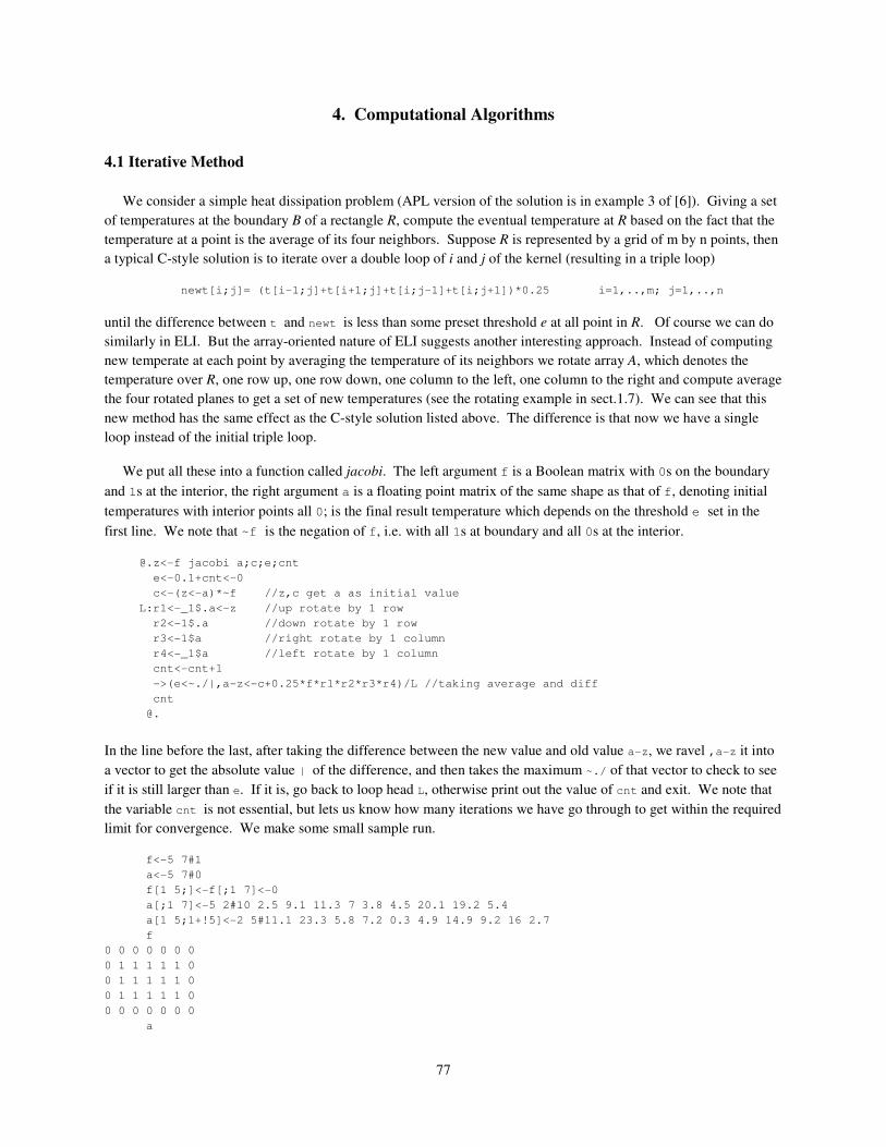
77
4. Computational Algorithms
4.1 Iterative Method
We consider a simple heat dissipation problem (APL version of the solution is in example 3 of [6]). Giving a set
of temperatures at the boundary B of a rectangle R, compute the eventual temperature at R based on the fact that the
temperature at a point is the average of its four neighbors. Suppose R is represented by a grid of m by n points, then
a typical C-style solution is to iterate over a double loop of i and j of the kernel (resulting in a triple loop)
newt[i;j]= (t[i-1;j]+t[i+1;j]+t[i;j-1]+t[i;j+1])*0.25 i=1,..,m; j=1,..,n
until the difference between t and newt is less than some preset threshold e at all point in R. Of course we can do
similarly in ELI. But the array-oriented nature of ELI suggests another interesting approach. Instead of computing
new temperate at each point by averaging the temperature of its neighbors we rotate array A, which denotes the
temperature over R, one row up, one row down, one column to the left, one column to the right and compute average
the four rotated planes to get a set of new temperatures (see the rotating example in sect.1.7). We can see that this
new method has the same effect as the C-style solution listed above. The difference is that now we have a single
loop instead of the initial triple loop.
We put all these into a function called jacobi. The left argument f is a Boolean matrix with 0s on the boundary
and 1s at the interior, the right argument a is a floating point matrix of the same shape as that of f, denoting initial
temperatures with interior points all 0; is the final result temperature which depends on the threshold e set in the
first line. We note that ~f is the negation of f, i.e. with all 1s at boundary and all 0s at the interior.
@.z<-f jacobi a;c;e;cnt
e<-0.1+cnt<-0
c<-(z<-a)*~f //z,c get a as initial value
L:r1<-_1$.a<-z //up rotate by 1 row
r2<-1$.a //down rotate by 1 row
r3<-1$a //right rotate by 1 column
r4<-_1$a //left rotate by 1 column
cnt<-cnt+1
->(e<~./|,a-z<-c+0.25*f*r1*r2*r3*r4)/L //taking average and diff
cnt
@.
In the line before the last, after taking the difference between the new value and old value a-z, we ravel ,a-z it into
a vector to get the absolute value | of the difference, and then takes the maximum ~./ of that vector to check to see
if it is still larger than e. If it is, go back to loop head L, otherwise print out the value of cnt and exit. We note that
the variable cnt is not essential, but lets us know how many iterations we have go through to get within the required
limit for convergence. We make some small sample run.
f<-5 7#1
a<-5 7#0
f[1 5;]<-f[;1 7]<-0
a[;1 7]<-5 2#10 2.5 9.1 11.3 7 3.8 4.5 20.1 19.2 5.4
a[1 5;1+!5]<-2 5#11.1 23.3 5.8 7.2 0.3 4.9 14.9 9.2 16 2.7
f
0 0 0 0 0 0 0
0 1 1 1 1 1 0
0 1 1 1 1 1 0
0 1 1 1 1 1 0
0 0 0 0 0 0 0
a

78
10 11.1 23.3 5.8 7.2 0.3 2.5
9.1 0 0 0 0 0 11.3
7 0 0 0 0 0 3.8
4.5 0 0 0 0 0 20.1
19.2 4.9 14.9 9.2 16 2.7 5.4
f jacobi r<-a
16
10 11.1 23.3 5.8 7.2 0.3 2.5
9.1 10.56506618 13.35146139 9.162343675 7.997351304 6.743705601 11.3
7 8.792694442 10.56761059 9.668714823 9.071017288 7.461734274 3.8
4.5 7.193014314 10.66325575 10.18157327 11.36247899 10.38498706 20.1
19.2 4.9 14.9 9.2 16 2.7 5.4
We see that it takes 16 iterations to get interior temperature to converge within 0.1. We would like to make e to
be a parameter so we can see how a change of that limit effect the number of iterations required. Thus the limit e
becomes the left parameter and the original left and right parameters are combined to be a list (f;a)as the new right
parameter in our newer version. We take this opportunity to eliminate the intermediate variables ri; and we modify
the last line slightly to print a header for the count variable cnt by glue it with format function (+.) applied to a
number to get its character representation.
[0] z<-e jacobi1 (a;f);c;e;cnt
[1] cnt<-0
[2] c<-(z<-a)*~f
[3] L:cnt<-cnt+1
[4] ->(e<~./|,a-z<-c+0.25*f*(_1$.a)+(1$.a)+(1$a)+_1$a<-z)/L
[5] 'count: ',+.cnt
0.1 jacobi1 (f;r)
count: 16
10 11.1 23.3 5.8 7.2 0.3 2.5
9.1 10.56506618 13.35146139 9.162343675 7.997351304 6.743705601 11.3
7 8.792694442 10.56761059 9.668714823 9.071017288 7.461734274 3.8
4.5 7.193014314 10.66325575 10.18157327 11.36247899 10.38498706 20.1
19.2 4.9 14.9 9.2 16 2.7 5.4
0.01 jacobi1 (f;r)
count: 26
10 11.1 23.3 5.8 7.2 0.3 2.5
9.1 10.66631246 13.53233886 9.364624216 8.177725139 6.844740327 11.3
7 8.94053114 10.81550314 9.963675573 9.318610663 7.608858719 3.8
4.5 7.294261178 10.84413374 10.38385498 11.54285334 10.48602238 20.1
19.2 4.9 14.9 9.2 16 2.7 5.4
We can even put this function in a more elegant form using control structures of ELI to avoid old APL fashioned
branching:
@.z<-e jacobi2 (f;a);c;cnt
cnt<-1
c<-(z<-a)*~f //z,c get a as initial value
while (e<~./|,a-z<-c+0.25*f*(_1$.a)+(1$.a)+(1$a)+_1$a<-z) cnt<-cnt+1
'count: ',+.cnt
@.
It is clear that array-oriented programming results in a very different style of program than traditionally C-style
loop-based program. Historically APL community developed array-oriented programming not just because APL
language encourages such thinking but also because the execution inefficiency of the APL interpreter severely
punishes loopy and non-succinct code. While the arrival of a good compiler can lessen such penalty it is precisely
programs of such style being most suitable for effective automatic parallelization by a parallelizing compiler without
introduction of additional parallel constructs alien to natural mathematical thinking in problem solving (see [6]).

79
4.2 Simple Encryption and Monte Carlo Method
4.2.1 encryption by random permutation
Recall the dyadic function deal A?.B, both A and B positive integers with A<=B; A?.B picks A distinct numbers
from !B we introduced in section 1.5 (please remember there is a ‘.’ after ‘?’ for random number generators)
10?.100
41 68 58 93 84 52 9 65 41 70
Now suppose A=B in above, say 26; the deal function would then result in a permutation of !B.
perm<-26?.26
alph<-'abcdefghijklmnopqrstuvwxyz'
alph[perm]
trqbpfisdnoemwvlgjkhcyzaxu
scrb<-alph[perm]
So we use a random permutation generated by an application of the deal function to scramble a text string as a
simple encryption tool. But how do we decrypt an encrypted text string at the receiving end? To this end we
introduce the primitive monadic sort function grade up (<) in ELI: for vector V, <V is a permutation of the indices
of V so that V[<V] is in a non-decreasing order.
V<-52 84 4 6 53 68 1 39 7 42
<V
7 3 4 9 8 10 1 5 6 2
V[<V]
1 4 6 7 39 42 52 53 68 84
The grade up <perm of the encryption permutation is the decryption key:
scrb[<perm]
abcdefghijklmnopqrstuvwxyz Now consider a more general case of a very long text string: to send a very long decryption key which is of the length of the text is certainly not practical. A reasonable solution is to designate a set of distinct characters as core to be scrambled and leave characters in the string which do not belong to the core to be left unchanged. To this end first let us work out the case that the plain text is a string of characters all belong to the core but with possible repetitions and not every character in core is in it. Say core is the lower case alphabets plus the space.
#core<-' abcdefghijklmnopqrstuvwxyz'
27
perm<-27?.27
perm
4 21 13 15 6 2 19 26 11 23 1 12 16 3 18 25 8 20 9 27 10 7 24 5 14 17 22
ptxt<-'i like to see you'
etxt<-core[perm[core!ptxt]]
etxt
vcovkacixczaacpxf where core!ptxt are positions of characters in ptxt in core and etxt is the encryption of ptxt. To decode it, we just apply the grade up function < to perm as before with encrypted core ecore replacing core:
ecore<-core[perm]
ecore
ctlnearyjv kobqxgshzifwdmpu

80
ecore[(<perm)[ecore!etxt]]
i like to see you Return to our original case that we have a large text lptxt with characters out of core, we need to remember the boolean vector w indicating which elements of lptxt are in core first to reduce lptxt to those in core for encryption and later to find positions in resulting string to be replaced by scrambled text. We illustrate this process with a sample lptxt:
lptxt<-'I like to see you at 11:00 pm today!'
iptxt<-(w<-lptxt?core)/lptxt //get those chars of lptxt which are in core
w
0 1 1 1 1 1 1 1 1 1 1 1 1 1 1 1 1 1 1 1 1 0 0 0 0 0 1 1 1 1 1 1 1 1 1 0
iptxt
like to see you at pm today
core[perm[core!iptxt]] //scramble iptxt
covkacixczaacpxfcticcgbcixetp
letxt<-lptxt
letxt[?w]<-core[perm[core!iptxt]] //?w indicates where iptxt sits inside letxt
letxt
Icovkacixczaacpxfctic11:00cgbcixetp! ?w indicates where elements of iptxt sit inside letxt and we replace them by scrambled text while leave the rest undisturbed. To decrypt, we first note that w also indicates which elements of letxt are in core and then we can just unscramble that portion of letxt to its original form:
letxt?core
0 1 1 1 1 1 1 1 1 1 1 1 1 1 1 1 1 1 1 1 1 0 0 0 0 0 1 1 1 1 1 1 1 1 1 0
w/letxt
covkacixczaacpxfcticcgbcixetp
ietxt<-w/letxt
ietxt
covkacixczaacpxfcticcgbcixetp
ietxt[(<perm)[ecore!ietxt]]
avcaaaocataaaxceacoaaxiaocccx
ecore
ctlnearyjv kobqxgshzifwdmpu
ecore!ietxt
1 13 10 12 6 1 21 16 1 20 6 6 1 26 16 22 1 2 21 1 1 17 14 1 21 16 5 2 26
(<perm)[ecore!ietxt]
11 3 21 12 5 11 2 13 11 18 5 5 11 8 13 27 11 6 2 11 11 26 25 11 2 13 24 6 8
ecore[(<perm)[ecore!ietxt]]
like to see you at pm today
letxt[?w]<-ecore[(<perm)[ecore!ietxt]]
letxt
I like to see you at 11:00 pm today!
We encapsulate the above computation into two functions: encrypt and decrypt. For the first function, its right argument is a pair of variables (core;perm), the core text to be scrambled and the random permutation used to encrypt, and its left argument is the text to be encrypted; the result is the encrypted text. For the second function, the right argument is the same as in the first function while the left argument is the encrypted message and the result is the recovered plain text. The first two lines of the function do suitability checking on the right argument.
@.z<-ptxt encrypt (core;perm);pl;w;iptxt
if (1~=##core) ->'core must be a vector'
if (~(pl=#=perm)^(#core)=pl<-#perm) ->'perm must of the same lgth as core with no duplicates'
iptxt<-(w<-ptxt?core)/z<-ptxt
z[?w]<-core[perm[core!iptxt]]
@.

81
@.z<-etxt decrypt (core;perm);pl;w;ietxt;ecore
if (1~=##core) ->'core must be a vector'
if (~(pl=#=perm)^(#core)=pl<-#perm) ->'perm must of the same lgth as core with no duplicates'
ecore<-core[perm]
ietxt<-(w<-etxt?core)/z<-etxt
z[?w]<-ecore[(<perm)[ecore!ietxt]]
@.
Let us try with slightly different variables:
#core<-' abcdefghijklmnopqrstuvwxyz0123456789'
37
perm<-37?.37
ptxt<-'Ms Evans, I like to see you at 11:00 pm today!'
emsg<-ptxt encrypt (core;perm)
emsg
MfaEysjf,aIadeztak aftta9 xaska22:qqaocak 0s9!
emsg decrypt (core;perm)
Ms Evans, I like to see you at 11:00 pm today! We note that repeat execution of n?.n in a workspace generates different permutations. So the encryption scheme can be looked upon as a one-time use pad. Still the need of send the permutation key to the receiving party of an encrypted message is not very safe. Hence modern encryption uses the RSA method based on public key encryption scheme. This method depends on the fact that knowing the product n of two very large prime numbers p and q it is computationally difficult to factorize n unless you know one of the primes.
4.2.2 Monte Carlo method to compute pi
Monte Carlo simulation is a computational method invented by Stanislow Ulam and John von Neumann during Manhattan Project. It is widely used in many situations where an analytic solution is not feasible such as in solving some partial differential equations and solving stochastic differential equations related to options pricing. At the heart of this method is using repeated random sampling to obtain numeric data. We illustrate this process by using the Monte Carlo method to find �, i.e. the value of @1.
In a 1 by 1 square Q, a quarter of the circle C inside Q consists of all points (x,y) such that √(x2+y
2)≤1. The basic
idea of the Monte Carlo method is to throw a large number of darts, say m, into Q and count the number of darts n which are inside C. Then the ratio n/m is approximately equal to the area of C, i.e. (n/m)=(1/4)� because the area of a circle is �r
2 where r is the length of the radius. Now the question is how do we generate a large number of
random darts in the unit square? We recall that monadic scalar function roll ?.n randomly generates a number between []IO and n-1+[]IO in sect. 1.5. Based on the roll function, we have the function rand n in standard.esf which gives n independent random numbers inside the unit interval [0,1]:
{rand: (?.x#1000000)%1000000} //independently gen. x numbers from 1..1M, then divide by 1M
rand 100
0.13153 0.75560 0.45865 0.53276 0.2189 0.04704 0.678865 0.679297 0.934693 0.383503 0.519417 0.830966
0.03457 0.05346 0.52970 0.6711 0.00769 0.38341 0.066843 0.417486 0.686773 0.588977 0.930437
0.84616 0.52693 0.09196 0.65392 0.416 0.701191 0.910321 0.762199 0.262453 0.047465 0.736082
0.32823 0.63264 0.75641 0.99104 0.36534 0.24704 0.98255 0.722661 0.753356 0.651519 0.072686
0.63163 0.88471 0.27271 0.43641 0.76649 0.47773 0.23777 0.274907 0.359265 0.166508 0.486518
0.89765 0.90921 0.06056 0.90465 0.50452 0.51629 0.31903 0.986643 0.493977 0.266145 0.090733
0.94776 0.07375 0.50071 0.38414 0.27708 0.91382 0.529748 0.464446 0.94098 0.050084 0.761515
0.77021 0.82782 0.12537 0.01587 0.68846 0.86825 0.629544 0.736225 0.72541 0.999458 0.888573
0.23319 0.30632 0.35102 0.51327 0.59111 0.84598 0.412081 0.841511 0.26932 0.415395 0.537304
To get random points in the unit square, we first generate their (x,y) coordinates, then compute their distance from
the origin (0,0) by introducing a simple length function and count how many of them are inside the circle.
x<-rand 100

82
y<-rand 100
{length:((x*.2)+y*.2)*.0.5}
length
3 length 4
5
3 4 length 4 5
5 6.403124237
dist<-x length y
#dist
100
dist
0.843825767 1.02808002 0.970931958 0.865037832 0.6406978738 0.965754676 0.5154958158 0.5443669671
0.647999475 1.11593778 1.15252348 0.707953201 1.15149743 1.07054072 1.10506844 0.8165047052
0.7378729788 1.030025732 0.1318180786 0.8906919036 0.5924622512 0.4633327123 0.4193921507
0.713929093 0.861922657 1.15128156 0.72301417 0.269342831 0.97007708 1.23955896 1.103319881
0.5643415876 0.6954200043 0.5930147851 1.062624391 0.5442390188 0.4697911129 0.6666902581
0.989885694 1.06079201 1.05174394 0.726557401 0.820142206 1.04891934 0.46025074 1.009132148
0.58541043 0.67903196 0.78647025 0.464031383 0.9610964 0.783555152 0.7542674995 0.451436771
0.755297341 0.6941582 0.941964123 0.654646899 1.1595364 0.750995766 0.95589978 0.4006316046
0.219070924 0.764531777 1.09971674 0.47710968 0.25646163 0.95094821 0.56528018 0.9611551484
1.297003305 0.4006022811 0.3143011801 0.6958074566 0.4627631845 0.8170429201 0.7954248035
0.8898329278 0.5356466962 0.3997390532 0.4524425589 0.8313774474 1.354537315 0.6958495927
0.847516659 0.69315699 0.99229927 0.650981749 0.878844029 0.953027188 0.52997251 1.15606853
0.857055143 0.7911189 0.473287146 0.97634126 0.89622853 0.823066743 1.14533233 0.9795147438
dist<=1
1 0 1 1 1 1 1 1 1 0 0 1 0 0 0 1 1 0 1 1 1 1 1 1 1 0 1 1 1 0 0 1 1 1 0 1 1 1 1 0 0 1 1 0 1 0 1 1 1
1 1 1 1 1 1 1 1 1 0 1 1 1 1 1 0 1 1 1 1 1 0 1 1 1 1 1 1 1 1 1 1 1 0 1 1 1 1 1 1 1 1 0 1 1 1 1 1 1
0 1
+/dist<=1
79
79%100
0.79
(@1)%4
0.7853981634
To get more accurate result, increase the number of darts, and this is a general approach in Monte Carlo simulation:
xl<-rand 10000
yl<-rand 10000
distl<-xl length yl
(+/distl<=1)%#distl
0.783
4.3 Sparse Matrix Computation
We have stated in section 1.8 that the inner product A+:*B for two matrices A and B is just the common dot-
product (matrix multiplication) of matrix A by matrix B, and for a vector x, A+:*x is the common matrix-by-vector
dot-product where the width of A must equal to the height of B or the length of x. For simplicity, we assume the
matrices we discuss in this section are all square matrices of size n. For example,
A
1.2 0 0 3 4.8
0 2.1 5 0 0
0 0 1 3.8 7
0 2 0 12 0
0.8 0 0 0 1.3
B
0 1 0 0 0
1 0 0 0 0

83
0 0 0 1 0
0 0 0 0 1
0 0 1 0 0
x<-9.1 3 4.5 0.7 8
A+:*B
0 1.2 4.8 0 3
2.1 0 0 5 0
0 0 7 1 3.8
2 0 0 0 12
0 0.8 1.3 0 0
A+:*x
51.42 28.8 63.16 14.4 17.68
We notice that B is a column permutation of the identity matrix I (i.e. I+:*A=A+:*I =A for all square matrices A)
1 0 0 0 0
0 1 0 0 0
0 0 1 0 0
0 0 0 1 0
0 0 0 0 1
and consequently A+:*B is a column permutation of A.
In general, for size n, to carry out the dot-product A+:*x the ELI inner product +:* needs to perform n2
multiplications and (n-1)*n additions. Usually in ELI/APL programming a programmer is not excessively
concerned about machine code execution efficiency while concentrating on the overall solution of a problem at hand.
But in the case of operations on very large matrices this a crucial question to consider. First, for n larger than
million or more, there is the question of how best to store the matrix in memory. In fact, many large matrices in real
applications arising from solutions to partial differential equations (see Saad [12]) are sparse, i.e. a large portion of
matrix A of size n are 0 in the sense that the number of non-zero elements in A is proportional to cn, for some
constant c, not n2. This implies that we only need to store non-zero elements of A and we can also skip operations
involve zero elements.
One of the methods to store nonzero elements of a sparse matrix is the compressed sparse row format (sect.3.4
[12]) or csr format. For a sparse matrix A of size n, this format comes with three vectors:
• a real (or complex) vector v of values of nonzero elements aij in A, row by row, with length cn.
• an integer vector c corresponding to vector v above with each element of c indicates the column number of
corresponding element aij; c is also of length cn.
• an integer vector p of length n+1 where each p[i] points to the beginning in v of nonzero elements of row
i for i from 1 to n and p[n+1]=cn+1.
For the specific matrix A in the example above, we have
v<-1.2 3 4.8 2.1 5 1 3.8 7 2 12 0.8 1.3
#v
12
c<-1 4 5 2 3 3 4 5 2 4 1 5
p<-1 4 6 9 11 13
To carry out a matrix-by-vector dot-product A+:*x of a sparse matrix A stored in csr format, we note that the i-th
row A of nonzero elements of A is v[p[i]..p[i+1]-1] where for the range p[i]..p[i+1]-1 we introduce a short
function range in ELI so x range y will yield x..y as its result:

84
{range:y+(-[]IO)+!1+x-y}
range
2 range1 5
2 3 4 5
The corresponding row elements of x involved in the operation is then x[c[p[i]range p[i+1]-1]]. Hence, for a
sparse matrix A stored in csr format (v;c;p) the following function carries out the matrix-by-vector operation for
vector x:
[0] y<-x spmatr_vec (v;c;p);n;idx;i
[1] y<-(n<-_1+#p)#0 //initialize y
[2] for (i:1;n){
[3] idx<-p[i] range p[i+1]-1
[4] y[i]<-v[idx]+:*x[c[idx]]
[5] }
x spmatr_vec (v;c;p)
51.42 28.8 63.16 14.4 17.68
A compressed sparse column format for a sparse matrix can be similarly defined but the function implementing
the matrix-by-vector operation differs from the above in line 4 (see Saad [12] sect. 3.4).
Many sparse matrices have mostly nonzero elements on their diagonal, or diagonal elements need to be accessed
more easily. Hence, for such a sparse matrix A of size n, we have a modified sparse raw (msr) format which has two
vectors dv and pc of the same length. The first n-elements of dv stores the value of diagonal elements of A, dv[n+1]
is not used, starting from position n+2, dv stores the nonzero elements of A excluding the diagonal, row by row.
The first n elements of pc store pointers to dv, i.e. each pc[i] points to the starting position of nonzero elements of
A in row i excluding the diagonal element with pc[n+1].=1+length of dv. Starting from position n+2, each pc[i]
stores the column index of the corresponding nonzero element dv[i] in certain row. We remark that in the rare case
that if for certain row i, all elements are zero other than the diagonal element, we need to stick in a 0 in dv for that
row with an arbitrary column number, say 1, in the corresponding position in pc. This is to maintain the uniformity
of processing code. For our given A above, we have the following vectors for its msr format:
dv<-1.2 2.1 1 12 1.3 _999 3 4.8 5 3.8 7 2 0.8
pc<-7 9 10 12 13 14 4 5 2 4 5 2 1
And the processing code for matrix-by-vector dot-product for a sparse matrix stored in mrs format is the following:
@.y<-x spmat_vec2 (dv;pc;n);idx;i
y<-x*n^.dv
for (i:1;n){
idx<-pc[i] range pc[i+1]-1
y[i]<-y[i]+dv[idx]+:*x[pc[idx]]
}
@.
X<-9.1 3 4.5 0.7 8
X spmat_vec2 (dv;pc;n)
51.42 21.3 63.16 14.4 17.68
85
References
[1] G. Blaauw, Digital System Implementation, Prentice Hall, 1976.
[2] H. Chen, W.-M. Ching, An ELI-to-C compiler: Production and performance, http://fastarray.appspot.com/, 2013.
[3] W.-M. Ching, Program analysis and code generation in an APL/370 compiler, IBM J. Res. Dev. 30, 594-605,
1986.
[4] W.-M. Ching, A Primer for ELI, a system for programming with arrays, http://fastarray.appspot.com/, 2013.
[5] W.-M. Ching, Z. Ju, An APL-to-C compiler for the IBM RS/6000: compilation, performance and limitations,
APL Quote Quad 23(3), 15-21, 1993.
[6] W.-M. Ching, D. Zheng: Automatic parallelization of array-oriented programs for a multi-core machine, Int. J.
Parallel Prog. 2012.
[7] D. Desrochers, Principles of Parallel and Multiprocessing, McGraw-Hill, 1983.
[8] G. Heineman, G. Pollice, S. Selkow, Algorithms in a Nutshell, O’Reilly, 2008.
[9] Int’l Organization for Standardization: ISO Draft Standard APL, APL Quote Quad 14(2),7-272, 1983.
[10] Ken. Iverson, Notation as a Tool of Thought, Comm. ACM, vol.23, no.8, 444-465, 1980.
[11] B. Kernighan and D. Richie, The C Programming Language, 2nd
ed., Prentice Hall, 1988.
[12] Y. Saad, Iterative Methods for Sparse Linear Systems, 2nd
ed., SIAM, 2003.
[13] N. Thomson, R. Polivka, APL2 in Depth, Springer-Verlag, 1995.
[14] N. Wirth, Algorithms + Data Structures = Programs, Prentice Hall, 1976.


