Introduction to Quantum Mechanics - ETH Zlnicolas/Files/QuantumMechanicsPVK/Quantum... · Nicolas...

Introduction to Quantum Mechanics

Nicolas [email protected]

1

Nicolas Lanzetti Quantum Mechanics FS 2017

Preface

This script in based on the lecture Introduction to Quantum Mechanics (FS 2017) for Engineerstaught by Pr. Dr. David Norris.

I cannot guarantee neither correctness nor completeness of the script. Please report any mistakedirectly to me.

Have fun with Quantum Mechanics!

June 20, 2017 Nicolas Lanzetti, [email protected]

2


Contents

1 The Wave Function and the Schrodinger Equation 51.1 The Schrodinger Equation . . . . . . . . . . . . . . . . . . . . . . . . . . . . . . . 51.2 Observables and Expectation Values . . . . . . . . . . . . . . . . . . . . . . . . . 51.3 Uncertainty Principle . . . . . . . . . . . . . . . . . . . . . . . . . . . . . . . . . . 61.4 The Time-independent Schrodinger Equation . . . . . . . . . . . . . . . . . . . . 71.5 General Solution to the TDSE . . . . . . . . . . . . . . . . . . . . . . . . . . . . 71.6 Free Particle . . . . . . . . . . . . . . . . . . . . . . . . . . . . . . . . . . . . . . 71.7 Confined Particle . . . . . . . . . . . . . . . . . . . . . . . . . . . . . . . . . . . . 81.8 Quantum Harmonic Oscillator . . . . . . . . . . . . . . . . . . . . . . . . . . . . . 81.9 Further Examples . . . . . . . . . . . . . . . . . . . . . . . . . . . . . . . . . . . . 10

1.9.1 Finite Potential Step . . . . . . . . . . . . . . . . . . . . . . . . . . . . . . 101.9.2 Finite Potential Well . . . . . . . . . . . . . . . . . . . . . . . . . . . . . . 101.9.3 Finite Potential Barrier . . . . . . . . . . . . . . . . . . . . . . . . . . . . 111.9.4 Quantum Mechanical Tunneling . . . . . . . . . . . . . . . . . . . . . . . 11

1.10 Quick Checks . . . . . . . . . . . . . . . . . . . . . . . . . . . . . . . . . . . . . . 121.11 Exercises . . . . . . . . . . . . . . . . . . . . . . . . . . . . . . . . . . . . . . . . 13

2 Formalism 222.1 Hermitian Operators . . . . . . . . . . . . . . . . . . . . . . . . . . . . . . . . . . 222.2 Dirac’s Notation . . . . . . . . . . . . . . . . . . . . . . . . . . . . . . . . . . . . 222.3 Quick Checks . . . . . . . . . . . . . . . . . . . . . . . . . . . . . . . . . . . . . . 232.4 Exercises . . . . . . . . . . . . . . . . . . . . . . . . . . . . . . . . . . . . . . . . 24

3 Measurements 263.1 Deterministic and Probabilistic Measurements . . . . . . . . . . . . . . . . . . . . 263.2 Commutator . . . . . . . . . . . . . . . . . . . . . . . . . . . . . . . . . . . . . . 263.3 Compatible Observables . . . . . . . . . . . . . . . . . . . . . . . . . . . . . . . . 273.4 Incompatible Observables . . . . . . . . . . . . . . . . . . . . . . . . . . . . . . . 273.5 Generalized Uncertainty Principle . . . . . . . . . . . . . . . . . . . . . . . . . . . 273.6 Time-energy Uncertainty Relation . . . . . . . . . . . . . . . . . . . . . . . . . . 283.7 Quick Checks . . . . . . . . . . . . . . . . . . . . . . . . . . . . . . . . . . . . . . 293.8 Exercises . . . . . . . . . . . . . . . . . . . . . . . . . . . . . . . . . . . . . . . . 30

4 Quantum Mechanics in 3D 364.1 The 3D Schrodinger Equation . . . . . . . . . . . . . . . . . . . . . . . . . . . . . 364.2 Hydrogen Atom . . . . . . . . . . . . . . . . . . . . . . . . . . . . . . . . . . . . . 364.3 Angular Momentum . . . . . . . . . . . . . . . . . . . . . . . . . . . . . . . . . . 364.4 Spin . . . . . . . . . . . . . . . . . . . . . . . . . . . . . . . . . . . . . . . . . . . 374.5 Quick Checks . . . . . . . . . . . . . . . . . . . . . . . . . . . . . . . . . . . . . . 394.6 Exercises . . . . . . . . . . . . . . . . . . . . . . . . . . . . . . . . . . . . . . . . 40

5 Systems with Multiple Particles 475.1 Atoms . . . . . . . . . . . . . . . . . . . . . . . . . . . . . . . . . . . . . . . . . . 475.2 Fermions and Bosons . . . . . . . . . . . . . . . . . . . . . . . . . . . . . . . . . . 475.3 Exchange Operator . . . . . . . . . . . . . . . . . . . . . . . . . . . . . . . . . . . 475.4 Pauli’s Exclusion Principle . . . . . . . . . . . . . . . . . . . . . . . . . . . . . . . 485.5 Multielectron Atoms . . . . . . . . . . . . . . . . . . . . . . . . . . . . . . . . . . 48

5.5.1 Electronic Configuration . . . . . . . . . . . . . . . . . . . . . . . . . . . . 485.6 Angular Momentum for Multiparticle Systems . . . . . . . . . . . . . . . . . . . . 49

5.6.1 Term Symbols . . . . . . . . . . . . . . . . . . . . . . . . . . . . . . . . . 49

3


5.6.2 Hund’s Rule . . . . . . . . . . . . . . . . . . . . . . . . . . . . . . . . . . . 495.7 Quick Checks . . . . . . . . . . . . . . . . . . . . . . . . . . . . . . . . . . . . . . 505.8 Exercises . . . . . . . . . . . . . . . . . . . . . . . . . . . . . . . . . . . . . . . . 51

6 Solids 586.1 Free Electron Model . . . . . . . . . . . . . . . . . . . . . . . . . . . . . . . . . . 58

6.1.1 Fermi Energy . . . . . . . . . . . . . . . . . . . . . . . . . . . . . . . . . . 586.1.2 Density of States . . . . . . . . . . . . . . . . . . . . . . . . . . . . . . . . 58

6.2 Kronig-Penny Model . . . . . . . . . . . . . . . . . . . . . . . . . . . . . . . . . . 586.2.1 Bloch’s Theorem . . . . . . . . . . . . . . . . . . . . . . . . . . . . . . . . 596.2.2 Metals . . . . . . . . . . . . . . . . . . . . . . . . . . . . . . . . . . . . . . 596.2.3 Insulators and Semiconductors . . . . . . . . . . . . . . . . . . . . . . . . 596.2.4 Doping . . . . . . . . . . . . . . . . . . . . . . . . . . . . . . . . . . . . . 60

6.3 Quick Checks . . . . . . . . . . . . . . . . . . . . . . . . . . . . . . . . . . . . . . 616.4 Exercises . . . . . . . . . . . . . . . . . . . . . . . . . . . . . . . . . . . . . . . . 62

7 Approximate Methods 657.1 Perturbation Theory . . . . . . . . . . . . . . . . . . . . . . . . . . . . . . . . . . 65

7.1.1 Non-degenerate Perturbation Theory . . . . . . . . . . . . . . . . . . . . . 657.1.2 Degenerate Perturbation Theory . . . . . . . . . . . . . . . . . . . . . . . 65

7.2 Variational Principle . . . . . . . . . . . . . . . . . . . . . . . . . . . . . . . . . . 657.3 Quick Checks . . . . . . . . . . . . . . . . . . . . . . . . . . . . . . . . . . . . . . 677.4 Exercises . . . . . . . . . . . . . . . . . . . . . . . . . . . . . . . . . . . . . . . . 68

A Probability Theory 73A.1 Normalization . . . . . . . . . . . . . . . . . . . . . . . . . . . . . . . . . . . . . . 73A.2 Expected Value . . . . . . . . . . . . . . . . . . . . . . . . . . . . . . . . . . . . . 73A.3 Variance . . . . . . . . . . . . . . . . . . . . . . . . . . . . . . . . . . . . . . . . . 73

B Dirac Delta Function 74

4


1 The Wave Function and the Schrodinger Equation

1.1 The Schrodinger Equation

Consider a particle of mass m that moves along the x-axis in a potential V (x, t). The particle’swave function Ψ(·, ·) : R× R→ C is the solution of the Schrodinger Equation (SE):

i~d

dtΨ = − ~2

2m

∂2Ψ

∂x2+ V (x, t)Ψ, (1.1)

where i2 = −1 and ~ = h/2π is the normalized Plank’s constant. The wave function has astatistical interpretation: ∫ b

aΨ∗Ψ dx =

∫ b

a|Ψ|2 dx = P (x(t) ∈ [a, b]), (1.2)

i.e. probability of finding the particle between a and b at time t (|Ψ|2 is the probability density).To be physically meaningful Ψ must be:

1. square-integrable: ∫ +∞

−∞|Ψ|2 dx <∞;

2. normalized: ∫ +∞

−∞|Ψ|2 dx = 1.

Remark. Square-integrability implies (at least in physics):

limx→±∞

Ψ = 0, limx→±∞

∂Ψ

∂x= 0.

Example. The wave function Ψ = kx with x ∈ R is not square integrable:∫ +∞

−∞|Ψ|2 dx =

∫ +∞

−∞k2x2 dx = 2

∫ +∞

0k2x2 dx→∞.

Example. The wave function Ψ = kx with x ∈ [−1,+1] is square-integrable and, for appropriatek, normalized:∫ +∞

−∞|Ψ|2 dx =

∫ +1

−1k2x2 dx = 2

∫ 1

0k2x2 dx =

2

3k2

!= 1 ⇒ k =

√3

2.

1.2 Observables and Expectation Values

Given any observable quantity Q, in QM we have an operator Q which can be written as afunction of the

• position operator: x = x and

• momentum operator p = −i~ ∂∂x ,

i.e. Q = Q(x, p). The expectation value of the quantity is

〈Q(x, p)〉 =

∫ +∞

−∞Ψ∗Q(x, p)Ψ dx. (1.3)

5


What does that mean? The expectation value of the position of the particle is

〈x〉 =

∫ +∞

−∞x|Ψ|2 dx.

The expectation value of the momentum is therefore

md〈x〉dt

= md

dt

∫ +∞

−∞x|Ψ|2 dx

= m

∫ +∞

−∞x

d

dtΨ∗Ψ dx

= m

∫ +∞

−∞x

(d

dtΨ∗Ψ +

d

dtΨΨ∗

)dx

= m

∫ +∞

−∞x

(− 1

i~

(− ~2

2m

∂2Ψ∗

∂x2+ VΨ∗

)Ψ +

1

i~

(− ~2

2m

∂2Ψ

∂x2+ VΨ

)Ψ∗)

dx

= m

∫ +∞

−∞

x

i~~2

2m

(∂2Ψ∗

∂x2Ψ− ∂2Ψ

∂x2Ψ∗)

dx

= m

∫ +∞

−∞

(− i~

2m

)x∂

∂x

(∂Ψ∗

∂xΨ− ∂Ψ

∂xΨ∗)

dx

= − i~2

(x

(∂Ψ∗

∂xΨ− ∂Ψ

∂xΨ∗) ∣∣∣+∞−∞−∫ +∞

−∞

(∂Ψ∗

∂xΨ− ∂Ψ

∂xΨ∗)

dx

)=i~2

(∫ +∞

−∞

∂Ψ∗

∂xΨ dx−

∫ +∞

−∞

∂Ψ

∂xΨ∗ dx

)=i~2

(Ψ∗Ψ

∣∣∣+∞−∞−∫ +∞

−∞

∂Ψ

∂xΨ∗ dx−

∫ +∞

−∞

∂Ψ

∂xΨ∗ dx

)= −i~

∫ +∞

−∞

∂Ψ

∂xΨ∗ dx

=

∫ +∞

−∞Ψ∗(−i~ ∂

∂x

)Ψ dx.

Thus, it holds p = −i~ ∂∂x .

Example. The kinetic energy operator is given by

T =1

2mv2 =

1

2

p2

m=

1

2m

(−i~ ∂

∂x

)(−i~ ∂

∂x

)= − ~2

2m

∂2

∂x2.

Remark. The expectation value is the (average) value we obtain if we measure the observableon a QM-ensemble (many identical particles with the same initial condition).

1.3 Uncertainty Principle

It holds:

σx · σp ≥~2, (1.4)

where σx is the standard deviation in x and σp the standard deviation in p.

Remark. The uncertainty principle is an inequality, i.e. σx · σp can be larger than ~/2.

6


1.4 The Time-independent Schrodinger Equation

Recall the time-dependent Schrodinger Equation (TDSE or SE):

i~d

dtΨ = − ~2

2m

∂2Ψ

∂x2+ V (x, t)Ψ. (1.5)

Assuming the potential is time independent, i.e. V (x, t) = V (x), and using separation of vari-ables with solutions

Ψ(x, t) = ψ(x)ϕ(t) (1.6)

we get

i~d

dtϕψ(x) = − ~2

2m

∂2ψ

∂x2ϕ(t) + V (x)ψ(x)ϕ(t)

i~1

ϕ(t)

d

dtϕ︸︷︷︸

LHS, C1(t)

= − ~2

2m

1

ψ(x)

∂2ψ

∂x2+ V (x)︸︷︷︸

RHS, C2(x)

= E

The LHS yields

i~1

ϕ(t)

d

dtϕ = E ⇒ ϕ(t) = exp(−iEt/~).

The RHS leads to the time-independent Schrodinger Equation (TISE):

Hψ(x) = Eψ(x), (1.7)

where

H = − ~2

2m

∂2

∂x2︸︷︷︸KE

+V (x)︸︷︷︸PE

(1.8)

is the Hamiltonian, i.e. the operator for the total energy. The full wave function is then

Ψn(x, t) = ψn(x) · exp(−iEnt/~). (1.9)

Remark. This is also called stationary state, since

|Ψn|2 = Ψ∗nΨn = ψ∗neiEnt/~ · ψne−iEnt/~ = ψ∗nψn = |ψn|2.

1.5 General Solution to the TDSE

The general solution is a linear combination of Ψn’s:

Ψ(x, t) =∞∑n=1

cnψn(x) exp(−iEnt/~). (1.10)

Remark. Stationary states are no longer possible, since |Ψ|2 leads to exp(i(Em−En)t/~) terms.

Remark. The probability that a measurement of energy will yield Ei is |ci|2.

1.6 Free Particle

Consider a free particle, i.e. V (x) = 0. The wave function is

Ψ(x, t) =1√2π

∫ +∞

−∞g(k) exp

(i

(kx− ~k2

2mt

))dk, (1.11)

where g(k) is the shape function

g(k) =1√2π

∫ +∞

−∞Ψ(x, 0) exp(−ikx) dx. (1.12)

Remark. The shape function is needed to make the solutions square-integrable (physical).

7


1.7 Confined Particle

Consider a particle in a infinite square well:

V (x) =

{0 if 0 ≤ x ≤ a,∞ else,

(1.13)

i.e. the particle can only be between 0 and a. The solutions to the TISE are

ψn(x) =

√2

asin(nπax), En =

n2π2~2

2ma2. (1.14)

a

x

V (x)

(a) Potential energy function.

a

E1

E2

E3

ψ1

ψ2

ψ3

x

E

(b) Wave functions.

Figure 1: Infinite Square Well.

Remark. The solutions to infinite square well are mutually orthogonal:∫ +∞

−∞ψ∗mψn dx = δmn =

{1 if m = n,

0 if m 6= n.

1.8 Quantum Harmonic Oscillator

Consider a particle in the potential V (x) = 12mω

2x2. The TISE yiels

− ~2

2m

∂2ψ

∂x2+

1

2mω2x2ψ = Eψ. (1.15)

To solve for ψn we introduce

a+ =1√

2~mω(−ip+mωx) = raising operator,

a− =1√

2~mω(+ip+mωx) = lowering operator.

(1.16)

Why? To make the TISE easier to solve. In particular, if ψ solves the TISE with energy E,then

Ha+ψ = (E + ~ω)a+ψ,

Ha−ψ = (E − ~ω)a−ψ,

8


i.e. a±ψ solves the TISE with energy E ± ~ω. From that:

a+ψn =√n+ 1ψn+1, ψ0 =

(mωπ~

) 14

exp(−mω

2~x2), En =

(n+

1

2

)~ω,

a−ψn =√nψn−1, ψn =

1√n!

(a+)nψ0,

where ψ0 comes from a−ψ = 0.

x

V (x)

(a) Potential energy function.

~ω

~ω

E0

E1

E2

x

E

(b) Wave functions.

Figure 2: Quantum Harmonic Oscillator.

Remark. In general, for ψ’s for confining potentials:

• If V (x) is symmetric, then ψn alternate even/odd;

• ψn+1 has one more node than ψn;

• ψn’s are mutually orthogonal, i.e.∫ +∞

−∞ψ∗mψn dx = δmn =

{1 if m = n,

0 if m 6= n;

• ψn’s make a complete set of functions, i.e. the general solution is a function of them.

• Orthogonality can be used to obtain the coefficients cn’s. By integrating

Ψ(x, 0) =

∞∑n=1

cnψn(x)

we obtain ∫ +∞

−∞ψ∗mΨ(x, 0) dx =

∫ +∞

−∞ψ∗m

∞∑n=1

cnψn dx =∞∑n=1

cn

∫ +∞

−∞ψ∗mψn dx.

Orthogonality then leads to

cm =

∫ +∞

−∞ψ∗mΨ(x, 0) dx.

9


1.9 Further Examples

To solve the problems with different potential the procedure is as follows:

• Divide the problem into regions and solve the TISE in each region.

• Use boundary conditions to match solutions at interfaces between regions. Typical bound-ary conditions are: continuity of ψ, ψ has to be finite, continuity of ∂ψ

∂x .

• For E > V (±∞) we have scattering states, for E < V (±∞) we have bound states.

Remark. Recall that for any solution it must hold: E > Vmin. Otherwise, the wave function isnot normalizable.

1.9.1 Finite Potential Step

Consider an incoming incident wave from left and a step of magnitude V0:

• E > V0: Reflection (QM behavior) and transmission wave.

• 0 < E < V0: Only reflection but penetration (QM behavior) into barriers.

• E < 0: No physical solutions.

V0

x

E

Figure 3: Finite Potential Step.

1.9.2 Finite Potential Well

Consider an incoming incident wave from left and a well of magnitude −V0 and width 2a:

• E > 0: Reflection (QM behavior) and transmission wave.

• −V0 < E < 0: Bound states with some penetration (QM behavior) into barriers.

• E < −V0: No physical solutions.

10


−a a

−V0

x

E

Figure 4: Finite Potential Step.

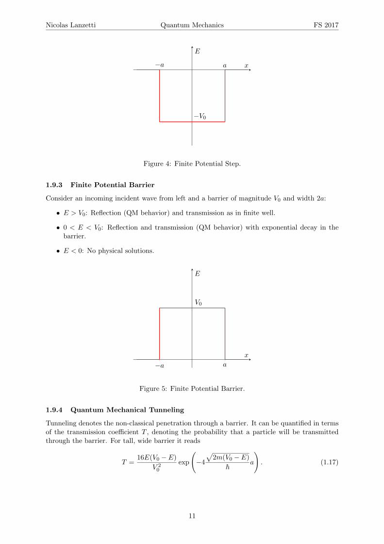
1.9.3 Finite Potential Barrier

Consider an incoming incident wave from left and a barrier of magnitude V0 and width 2a:

• E > V0: Reflection (QM behavior) and transmission as in finite well.

• 0 < E < V0: Reflection and transmission (QM behavior) with exponential decay in thebarrier.

• E < 0: No physical solutions.

−a a

V0

x

E

Figure 5: Finite Potential Barrier.

1.9.4 Quantum Mechanical Tunneling

Tunneling denotes the non-classical penetration through a barrier. It can be quantified in termsof the transmission coefficient T , denoting the probability that a particle will be transmittedthrough the barrier. For tall, wide barrier it reads

T =16E(V0 − E)

V 20

exp

(−4

√2m(V0 − E)

~a

). (1.17)

11


1.10 Quick Checks

Circle True or False.

T F Ψ(x, t) has no direct physical meaning.

T F According to the uncertainty principle, if σx is very large, then the momentumis well determined.

T F Any solution of the T.I.S.E. can be normalized.

T F To obtain the T.I.S.E. from the T.D.S.E., we had to assume that the potentialenergy function was time-independent.

T F If we confine an electron inside a finite volume with V (x) = 0, its ground stateenergy can never be exactly zero.

T F Stationary states have a probability density that does not change with time.

T F If a particle is described by a wave packet, its energy is always well defined.

T F ddt

∫ +∞−∞ |Ψ(x, t)|2 dx = 0 arises only for unphysical solutions to the 1D SE.

T F∫ +∞−∞ |Ψ(x, t)|2 dx = 0 arises only for unphysical solutions to the 1D SE.

T F It holds 〈H2〉 =(∑

i |ci|2Ei)2

.

T F It holds 〈H2〉 =(∑

i |ci|2E2i

).

12


1.11 Exercises

1. Given the two square wells as shown below with the same width.

(a) Sketch the ground state wavefunction in the corresponding plot.

(b) Sketch the first excited state. Assume that V0 is large.

a

x

V (x)

−a a

V0

x

E

13


2. Consider a particle in the infinite square well with an initial wave function:

Ψ(x, 0) = A(ψ1(x) + ψ2(x)).

(a) Normalize Ψ(x, 0).

(b) Determine Ψ(x, t) and |Ψ(x, t)|2.(c) Compute 〈x〉.(d) Compute 〈p〉.(e) If you measure the energy of this particle, what are the possible values?

(f) What is the probability of obtaining each of the possible energies?

(g) Compute 〈H〉 and compare to E1 and E2.

14


15


3. Consider a free particle with an initial normalized wave function:

Ψ(x, 0) =

(2a

π

) 14

exp(−ax2),

where a is a real positive constant.

(a) Determine Ψ(x, t).

(b) Determine |Ψ(x, t)|2.(c) Sketch |Ψ(x, t)|2 versus x at t = 0 and at a later t. Describe qualitatively what

happens to |Ψ(x, t)|2 as a function of time.

(d) Find σx and σp.

(e) Is the uncertainty principle satisfied?

(f) At what time does the system come closest to the uncertainty principle?

Hint: ∫ +∞

−∞e−(ax

2+ikx) dx =

√π

ae−

k2

4a .

16


17


4. We prepare a simple harmonic oscillator with the following normalized wavefunction:

Ψ(x, 0) =

(9β2

π

) 14

exp(−9(βx)2/2),

where β =√mω/~. We then immediately measure the energy of the oscillator in this

state. What is the probability of getting the ground state energy?

18


19


5. Give an example of a quantum mechanical system that has both a discrete and continuouspart to its spectrum.

20


6. At time zero, a system is in a linear combination:

Ψ =√

2ψ1 +√

3ψ2 + ψ3 + ψ4,

where ψn represents a normalized eigenstate of the system’s Hamiltonian H such that

Hψn = n2εψn.

If the energy of the system is measured at time zero, what values will be obtained andwith what probabilities?

21


2 Formalism

2.1 Hermitian Operators

In quantum mechanics, operators are linear and Hermitian. An operator Q is linear if

Q(αf(x) + βg(x)) = αQf(x) + βQg(x), (2.1)

where α, β ∈ R. An operator Q is Hermitian if∫ +∞

−∞Ψ∗QΨ d3~r =

∫ +∞

−∞(QΨ)∗Ψ d3~r (2.2)

or, using Dirac’s notation,〈Ψ|QΨ〉 = 〈QΨ|Ψ〉.

Remark. Note that the two following statements are equivalent:

• 〈Ψ|QΨ〉 = 〈QΨ|Ψ〉;

• 〈f |Qg〉 = 〈Qf |g〉.

Example. Consider the operator Q = a, where a ∈ R \ {0}. Then,

〈f |Qg〉 =

∫ +∞

−∞f∗Qg dx =

∫ +∞

−∞f∗ag dx =

∫ +∞

−∞af∗g dx =

∫ +∞

−∞(af)∗g dx = 〈Qf |g〉.

Thus, Q = a is Hermitian.

Example. Consider the operator Q = i. Then,

〈f |Qg〉 =

∫ +∞

−∞f∗Qg dx =

∫ +∞

−∞f∗ig dx =

∫ +∞

−∞if∗g dx =

∫ +∞

−∞(−(if)∗)g dx = −〈Qf |g〉.

Thus, Q = i is not Hermitian.

2.2 Dirac’s Notation

In general,

〈f |g〉 =

∫ +∞

−∞f∗g dx ∈ R.

Why does that make sense?〈f | is a row matrix:

〈f | =[c∗1 c∗2 . . . c∗n

]and |f〉 is a column matrix:

|f〉 =

c1c2...cn

.Thus, it makes sense that

〈f |f〉 =[c∗1 c∗2 . . . c∗n

]c1c2...cn

=

n∑i=1

|ci|2 ∈ R.

22


2.3 Quick Checks


T F The momentum operator p is not Hermitian, since p 6= p∗.

T F The Dirac Delta function is not in Hilbert space.

T F The function f(x) = sin(x) is in Hilbert space.

T F The function f(x) = e−x sin(x) is in Hilbert space.

T F The function f(x) = e−x4

sin(x) is in Hilbert space.

T F Every classical observable can be represented in QM by a Hermitian Operator.

T F The operator A = diag(4, 4, 2) is Hermitian.

T F The operator A = diag(4, 4, i) is Hermitian.

T F For a free particle, the separable solutions to the SE are not in Hilbert space.

23


2.4 Exercises

1. (a) Show that the sum of two Hermitian operators is Hermitian.

(b) When is the product of two Hermitian operators also Hermitian?

24


2. Consider a particle in the infinite square well constrained to have n ≤ 3.

(a) Write the general wavefunction in vector notation (as braket).

(b) Write the Hamiltonian of the system in matrix form.

25


3 Measurements

3.1 Deterministic and Probabilistic Measurements

A measurement of a quantity Q is deterministic iff Var[Q] = σ2Q

= 0. That is,

σ2Q

= 〈(Q− 〈Q〉)2〉

= 〈Ψ|(Q− 〈Q〉)2Ψ〉= 〈(Q− 〈Q〉)Ψ|(Q− 〈Q〉)Ψ〉

=

∫ ((Q− 〈Q〉)Ψ

)∗(Q− 〈Q〉)Ψ d3~r

=

∫ ∣∣(Q− 〈Q〉)Ψ∣∣2 d3~r!

= 0.

That holds if and only if (Q− 〈Q〉)Ψ = 0, i.e. Ψ satisfies the eigenvalue equation

QΨ = qQΨ, (3.1)

where qQ = 〈Q〉. In general, an equation of the form

Qfq = qfq

is called eigenvalue equation, where q is an eigenvalue of Q and fq is the corresponding eigen-function.

Example. Consider a particle in the infinite square well with Ψ = Ψ1. We investigate whethermeasurements of the energy are deterministic:

HΨ = HΨ1 = E1Ψ1.

Therefore, measurements are deterministic.

Example. Consider a particle in the infinite square well with Ψ = Ψ1. We investigate whethermeasurements of the position are deterministic:

xΨ = xΨ1 6= qxΨ1.

Therefore, measurements are probabilistic.

Example. Consider a particle in the infinite square well with Ψ = 1√2(Ψ1 +Ψ2). We investigate

whether measurements of the energy are deterministic:

HΨ = H

(1√2

(Ψ1 + Ψ2)

)=

1√2

(E1Ψ1 + E2Ψ2) 6= qHΨ.

Therefore, measurements are probabilistic.

3.2 Commutator

Consider two operators A and B. The commutator of A and B is

[A, B] = AB − BA. (3.2)

To evaluate it place a function to the right and then eliminate it.

Remark. If A and B commute then [A, B] = 0.

26


Example. Consider A = x and B = c, where c ∈ R. Then,

[A, B]f(x) = (x~− ~x)f(x) = x~f(x)− ~xf(x) = 0 · f(x).

Thus, [A, B] = 0.

Example. Consider A = x and B = ∂∂x , where c ∈ R. Then,

[A, B]f(x) =

(x∂

∂x− ∂

∂xx

)f(x) = x

∂f(x)

∂x−∂(xf(x))

∂x= x

∂f(x)

∂x−(f(x) + x

∂f(x)

∂x

)= −f(x)

Thus, [A, B] = −1.

3.3 Compatible Observables

Two observables A and B are called compatible if

[A, B] = 0.

Two compatible observables share the same eigenfunctions:

A|ψn〉 = an|ψn〉,B|ψn〉 = bn|ψn〉.

As a consequence, we can determine both observables at the same time.

3.4 Incompatible Observables

Two observables A and B are called incompatible if

[A, B] 6= 0.

Two incompatible observables have different eigenfunctions:

A|ψn,A〉 = an|ψn,A〉,B|ψm,B〉 = bm|ψm,B〉.

As a consequence, we cannot determine both observables at the same time.

Example. x and p are incompatible observables, since [x, p] = i~ 6= 0. x and y are compatibleobservables, since they commute.

3.5 Generalized Uncertainty Principle

The uncertainty principle for two observables A and B is

σ2Aσ2B≥(

1

2i〈[A, B]〉

)2

. (3.3)

Example. For A = x and B = p we obtain

σ2Aσ2B≥(

1

2i〈[x, p]〉

)2

=

(1

2i〈i~〉

)2

=

(1

2ii~)2

=

(~2

)2

,

which gives the well-known expression σxσp ≥ ~/2.

27


3.6 Time-energy Uncertainty Relation

The time-energy uncertainty relation is

σ2Hσ2Q≥(~2

)2(d〈Q〉dt

)2

. (3.4)

From that, using

∆E = σH , ∆t =σQ∣∣d〈Q〉dt

∣∣ ,we obtain ∆E∆t ≥ ~/2.

Remark. This uncertainty relation cannot be derived from the generalized uncertainty principle.

28


3.7 Quick Checks


T F In quantum mechanics, all measurements are probabilistic.

T F Two Hermitian operators always commute.

T F If a particle is in a non-stationary state, the measurement of its energy must yieldone of several values.

T F If a quantum mechanical observable is measured, one possible result is always theexpectation value of the observable.

T F An uncertainty relation will exist for any two observables that have operatorsthat do not commute.

T F px and py are compatible observables.

T F Since V = V (x) and [x, p] 6= 0, the operators p and V never commute.

29


3.8 Exercises

1. An operator A, representing observable A, has two normalized eigenstates ψ1 and ψ2

with eigenvalues a1 and a2, respectively. Operator B, representing observable B, has twonormalized eigenstates φ1 and φ2 with eigenvalues b1 and b2 respectively. The eigenstatesare related by

ψ1 =1

5(3φ1 + 4φ2)

ψ2 =1

5(4φ1 − 3φ2).

(a) Observable A is measured, and the eigenvalue a2 is obtained. What is the state ofthe system immediately after this measurement?

(b) If observable B is now measured (after the first measurement in part (a)), what arethe possible results, and what are their probabilities?

(c) Right after the measurement of B in part (b), A is measured again. You were nottold the outcome of the B measurement before the A measurement. What is theprobability of getting a2 after the three measurements (A, B, and then A)?

(d) Would your answer in part (c) change if you were told the outcome of the B mea-surement? How?

30


31


2. Determine [a−, a+].

32


3. Is the ground state of the infinite square well an eigenfunction of momentum? If so, whatis its momentum? If not, why not?

33


4. Below is a set of one-dimensional operators for a particle in an arbitrary potential V (x).Identify the largest group of compatible observables.

x, p, V (x), a+, H.

34


5. Determine eigenvalues and eigenvectors of Q = ∂∂x . Which eigenfunctions of Q are in

Hilbert space?

35


4 Quantum Mechanics in 3D

4.1 The 3D Schrodinger Equation

The 3D Schrodinger equation is given by

i~d

dtΨ = −−~

2

2m∇2Ψ + VΨ. (4.1)

Similarly as in the 1D, we assume the potential is time-independent. Then, we can use separationof variable and obtain the TISE

Hψ = Eψ, (4.2)

where H = − ~22m∇

2 + V .

4.2 Hydrogen Atom

For the hydrogen atom the potential is given by Coulomb attraction. That is,

V (r) = − e2

4πε0

1

r.

By rewriting the TISE in spherical coordinates we obtain

ψn,l,ml= Rn,l(r)Y

mll (θ, ϕ), (4.3)

where Rn,l(r) and Y mll (θ, ϕ) can be found in tables. The energy levels are

En = − 1

n2

(m

2~2

(e2

4πε0

)2)≈ −13.6 eV

n2. (4.4)

We can also define the Bohr radius, denoted by a and given by

a =4πε0~2

me2≈ 0.0529 nm.

Remark. Since En’s are discrete only the photon energies E2−E1, E3−E1, . . . can be absorbedby the hydrogen atom.

4.3 Angular Momentum

For the angular momentum we use the classic definition:

Lx = ypz − zpy, Ly = zpx − xpz, Lz = xpy − ypx, L2 = L2x + L2

y + L2z.

We have seen that Lx, Ly, and Lz do not commute, but they all commute with L2. Theeigenfunctions are the spherical harmonics and the eigenvalues are function of l:

L2Y mll = ~2l(l + 1)Y ml

l ,

LzYmll = ~mlY

mll ,

(4.5)

where l = 0, 1, 2, . . . and ml = −l,−l + 1, . . . , l − 1, l.

36


4.4 Spin

Due the intrinsic spin of the particle, it acts as if it has an inherent rotation about z-axis.Similarly to the angular momentum the eigenvalue problem is:

S2|s,ms〉 = ~2s(s+ 1)|s,ms〉,Sz|s,ms〉 = ~ms|s,ms〉.

(4.6)

for s = 0, 12 , 1,32 , . . . and ms = −s,−s+ 1, . . . , s− 1, s.

Remark. For an electron: it can occupy different orbitals, so l can vary (s, d, p, . . . orbitals).However, each quantum mechanical particle has a fixed spin s. For an electron s = 1

2 , for aphoton s = 1.

Therefore, for an electron (or any 12 -spin particle) there are two possible eigenstates:

|s,ms〉 →

{|12 ,+

12〉 “spin up”,

|12 ,−12〉 “spin down”,

(4.7)

where up/down refer to the projection of the spin along the z-axis. We can choose theseeigenstates as our basis vectors, that is

|12 ,+12〉 →

[10

],

|12 ,−12〉 →

[01

].

(4.8)

Then, the general spin state can be written as a linear combination:

|χ〉 = a|12 ,+12〉+ b|12 ,−

12〉,

|χ〉 = a

[10

]+ b

[01

],

|χ〉 =

[ab

] (4.9)

The operators in this basis are given by

S2 =3

4~2[1 00 1

], Sz =

~2

[1 00 −1

], Sx =

~2

[0 11 0

], Sy =

~2

[0 −ii 0

].

Example. Let’s work out S2. We know it is a 2× 2 matrix, that is

S2 =

[c de f

].

We use the eigenvalue equations:

S2|12 ,±12〉 = ~2s(s+ 1)|12 ,±

12〉

= ~21

2

(1

2+ 1

)|12 ,±

12〉

=3

4~2|12 ,±

12〉.

In matrix notation: [c de f

] [10

]=

3

4~2[10

]⇒

[ce

]=

3

4~2[10

].

37


Thus, c = 34~

2 and e = 0. Similarily[c de f

] [01

]=

3

4~2[01

]⇒

[df

]=

3

4~2[01

],

which leads to d = 0 and f = 34~

2. Hence,

S2 =3

4~2[1 00 1

].

Example. Consider a particle with spin 2. The possible values of ms are {−2,−1, 0, 1, 2}.Therefore, there are 5 eigenstates, given by |2,±2〉, |2,±1〉, and |2, 0〉. In vector form we wouldhave 5-dimensional vectors/matrices.

38


4.5 Quick Checks


T F Given a specific shell in a hydrogenic atom, all of the subshells have the sameenergy.

T F The orbital shapes that we know from chemistry (s, p, d, etc.) come from thesolutions to the angular equation of the hydrogen atom.

T F For a single-particle system with a spherically symmetric potential, the eigen-

functions of H will involve the spherical harmonics.

T F In our mathematical treatment of the hydrogen atom, the potential energy func-tion only affected the radial equation.

T F Each spin eigenstate can be represented as a two-dimensional vector.

T F For an atom with two electrons we can solve the TISE exactly (using separationof variables) if we ignore the interaction between the particles.

T F For an one-electron atom with the potential V (r, t) = e2

4πε01r cos(ωt) we can solve

the TISE exactly.

T F For an electron, the value of s can be ±12 .

T F Lx and L2 are compatible observables .

T F The electron has a spin angular momentum because it is rotating in space.

T F If we excite an electron in a hydrogen atom, we can change both its s and l.

T F If we state that the spin of an electron is “up” with respect to the z axis, thismeans its spin-angular-momentum vector is pointing parallel to the z axis.

T F An electron cannot be both “spin up” and “spin down”.

39


4.6 Exercises

1. If a particle is placed in a sphere of radius ρ where the potential V (r) is described by

V (r) =

{0 for r ≤ ρ,∞ for r > ρ,

where r is radial coordinate. Write down the angular components to the particles wavefunction.

40


2. A hydrogenic atom consists of a single electron orbiting a nucleus with Z protons. Forexample, Z = 1 for hydrogen itself, Z = 2 for helium with one electron removed, Z = 3 forlithium with two electrons removed, etc. Determine the Bohr energies En(Z), the bindingenergy E1(Z), and the Bohr radius a(Z) for a hydrogenic atom.

41


3. We introduced a specific spin 1/2 basis in lecture, i.e.,

|12 ,+12〉 →

[10

], |12 ,−

12〉 →

[01

],

where the ket notation represents |s,ms〉.

(a) In this basis, determine the eigenvalues and eigenvectors for Sy.

(b) If you measure Sy on the general spin state

|χ〉 = a

[10

]+ b

[01

],

what values would you get and with what probabilities? Check that the probabilitiesadd to one.Note: a and b do not have to be real.

(c) If you measure S2y on the same general state, what values would you get and with

what probabilities?

42


43


4. Consider a particle in the orbital angular momentum

ψ =

√2

7Y 11 +

√2

7Y −11 +

√1

14Y 00 +

√1

14

2∑i=−2

Y i2 .

(a) What are the possible values for a measurement of Lz? What is 〈Lz〉?(b) What are the possible values for a measurement of L2? What is 〈L2〉?

44


5. (a) Determine [Lz, r2] where r2 = x2 + y2 + z2.

Hint: Use your knowledge (or cheat sheet) for [Lz, x], [Lz, y], [Lz, z].

(b) Determine [Lz, p2] where p2 = p2x + p2y + p2z.

Hint: Use your knowledge (or cheat sheet) for [Lz, px], [Lz, py], [Lz, pz].

(c) Show that the Hamiltonian H commutes with all three components of L if the poten-tial is spherically symmetric. Thus, H, L2, Lz all commute. What is the significanceof this?

45


46


5 Systems with Multiple Particles

5.1 Atoms

Consider an atom with Z electrons and Z protons. Then,

H =

Z∑j=1

(− ~2

2m∇2j −

1

4πε0

Ze2

|~rj |

)︸︷︷︸H of j-th electron in hydr. state

+1

2

1

4πε0

Z∑k=1,k 6=j

e2

|~rj − ~rk|︸︷︷︸interaction between electrons

. (5.1)

The second term causes a mathematical problem: We can no longer solve the S.E. exactly.First, we neglect this term. Then electrons are each sitting in single-particle hydrogenic state.However, electrons are indistinguishable, therefore we have to consider linear combinations. Byassuming there are only two particles, we get:

Spatial:ψ± = C (ψa(~r1)ψb(~r2)± ψb(~r1)ψa(~r2)) (5.2)

ψ± is the two particle state (spatial part of the wave function).

Spin:

χ(s) =

↑↑ ⇒ Triplet

↓↓ ⇒ Triplet1√2(↑↓ + ↓↑) ⇒ Triplet

1√2(↑↓ − ↓↑) ⇒ Singlet

(5.3)

The first three states are called triplet (symmetric), the last one singlet (anti-symmetric).

The overall wave function will be the product of spatial and spin parts.

5.2 Fermions and Bosons

A fermion is a QM particle with half-integer spin, a boson is a QM particle with integer spin.Thus, electrons are fermions.Axiom: The overall wave function for a multiple particle system of identical fermions must beantisymmetric with respect to exchange of any two particles. For bosons, it must be symmetric.So for an electron (fermion), the overall wave function is

ψ+ · (singlet) or ψ− · (triplet).

5.3 Exchange Operator

Define the exchange operator:P f(~r1, ~r2)→ f(~r2, ~r1) (5.4)

This operator switches the position of two particles. Note that [P , H] = 0, i.e. P and H sharethe same eigenfunctions ψ+ and ψ−. The eigenvalues are ±1.

47


5.4 Pauli’s Exclusion Principle

There is no way to place two electrons in exactly the same state (i.e. with the same n, l,ml,ms)and still have an antisymmetric state.Motivation: Assume two fermions share the same quantum numbers. Then,

ψ+ = C (ψn,l,ml(~r1)ψn,l,ml

(~r2) + ψn,l,ml(~r1)ψn,l,ml

(~r2)) ,

= 2Cψn,l,ml(~r1)ψn,l,ml

(~r2)

ψ− = C (ψn,l,ml(~r1)ψn,l,ml

(~r2)− ψn,l,ml(~r1)ψn,l,ml

(~r2))

= 0.

In order to obtain a physical solution, we must therefore pick ψ+. Thus, the spin must beantisymmetic(singlet) in order to have an antisymmetric wave function; that is

χms =1

2(↑↓ − ↓↑).

With a triplet (in particular ↑↑ or ↓↓) the overall wave function cannot be antisymmetric.Therefore, the two electrons cannot share the same quantum numbers.

5.5 Multielectron Atoms

Recall the quantum numbers n, l,ml,ms:

• n designates the shell of electron orbital, n = 1, 2, . . .;

• l designates the subshell (shape) of electron orbital, l = 0, . . . , n− 1;

• ml designates the orientation of orbital, ml = −l, . . . , l;

• ms designates the spin of electron (up or down), ms = ±12 .

In the hydrogenic states the energies are

En = − 1

n2

(m

2~2

(Ze2

4πε0

)2),

i.e. subshells are degenerate (e.g. n = 1, l = 1 and n = 1, l = 0). For multielectron atomsdifferent subshells are not degenerate, due to screening (electron-electron interactions).

5.5.1 Electronic Configuration

To indicate how an atom is filled we can use the electronic configuration.

Example. Determine the electronic configuration:

• Ar, Z = 18, 1s22s22p63s23p6.

• Cl, Z = 17, 1s22s22p63s23p5

• Fe, Z = 26, [Ar]4s23d6.

Exceptions: Cr, Cu.

48


5.6 Angular Momentum for Multiparticle Systems

Define the new quantum numbers:

• L: total orbital angular momentum, ML =∑

imli ;

• S: total spin angular momentum, MS =∑

imsi ;

• J : total angular momentum, combines L and S;

• MJ = ML +MJ .

Remark. Filled subshells never contribute to L, S, J , since ML =∑

imli = 0 and MS =∑imsi = 0, which is the case only for L = S = 0. Thus, J = 0.

What does combine mean?Given any two angular momenta in QM:

j1 and j2combine to give⇒ j.

The possible values are

j = (j1 + j2), (j1 + j2 − 1), . . . , |j1 − j2|.

Example. Let j1 = 4, j2 = 4. Then j = 8, 7, 6, 5, 4, 3, 2, 1, 0.

Example. Let j1 = 3, j2 = 52 . Then j = 11

2 ,92 ,

72 ,

52 ,

32 ,

12 .

5.6.1 Term Symbols

For any element we can consider the electronic configuration and determine all the possiblecombinations of angular momenta. These are labeled by the term symbols:

2S+1LJ , (5.5)

where L = 0 ≡ “S”, L = 1 ≡ “P”, L = 2 ≡ “D”, and L = 3 ≡ “F”.

Example. What are the possible term symbols for Al? The electronic configuration is [Ne]3s23p1.Thus, only one electron will determine the total angular momentum. Since l = 1 we have L = 1.Similarly, since s = 1

2 we have S = 12 . The possible values of J are then 3

2 ,12 . Therefore, the

possible term symbols are2P 3

2,2 P 1

2.

5.6.2 Hund’s Rule

To determine the ground state we can use Hund’s Rules:

1. The state with the largest S is the most stable;

2. For states with the same S the largest L is most stable;

3. For states withe the same S and L:

• smallest J is most stable for subshells less or equal than half full;

• largest J is most stable for subshells more than half full.

49


5.7 Quick Checks


T F In a multielectron atom with two electrons in 2p orbital the possible values of Lare 0, 1, 2.

T F Given a system of two identical particles, the exchange operator P always com-

mute with the Hamiltonian operator H.

T F The Pauli exclusion principle applies to both fermions and bosons.

T F In quantum mechanics, an electron and proton are always distinguishable.

T F Quantum mechanics allows us to determine the length of the orbital angularmomentum vector.

T F The Pauli’s principle applies to particles with s = 32 .

T F The electron configuration of an atom (e.g.1s22s22p2) is enough information todescribe its exact energy.

T F In multielectron atoms, the 3p orbitals are lower in energy than the 4s orbitals.

T F In multielectron atoms, the 3d orbitals are lower in energy than the 4s orbitals.

T F It is possible to have the following term symbol for a multielectron atomic state:1D1.

T F The term symbol for J = 2, L = 1, and S = 1 is 1D1.

T F For multielectron atoms, the energy of the single-particle states only depends onn.

50


5.8 Exercises

1. Answer the following questions:

(a) Which of the following combinations of quantum numbers are allowed for a single-particle hydrogenic state?

� n = 3, l = 2,ml = 1,ms = 0.

� n = 2, l = 0,ml = 0,ms = −1/2.

� n = 7, l = 2,ml = −2,ms = 1/2.

� n = 3, l = −3,ml = −2,ms = −1/2.

� n = 0, l = 0,ml = 0,ms = 1/2.

(b) Determine the electronic configurations for the following elements:

• B: . . . . . . . . . . . . . . . . . . . . . . . . . . . . . . . . . . . .

• F: . . . . . . . . . . . . . . . . . . . . . . . . . . . . . . . . . . . .

• P: . . . . . . . . . . . . . . . . . . . . . . . . . . . . . . . . . . . .

• C: . . . . . . . . . . . . . . . . . . . . . . . . . . . . . . . . . . . .

• Cr: . . . . . . . . . . . . . . . . . . . . . . . . . . . . . . . . . . . .

• Ma: . . . . . . . . . . . . . . . . . . . . . . . . . . . . . . . . . . . .

• Fe: . . . . . . . . . . . . . . . . . . . . . . . . . . . . . . . . . . . .

• Cu: . . . . . . . . . . . . . . . . . . . . . . . . . . . . . . . . . . . .

• Kr: . . . . . . . . . . . . . . . . . . . . . . . . . . . . . . . . . . . .

51


2. Using the rules for the addition of angular momenta (i.e. do not worry about exchangesymmetry), determine all the possible electronic states for the elements B, C, and N interms of their possible “term symbols”, i.e. 2S+1LJ , where S is the total electronic spin,L is the total orbital angular momentum, and J is the total angular momentum.

52


53


3. What is the electronic configuration and term symbol for the ground state of Al?

54


4. Find the ground-state energy for a system of N noninteracting identical particles that areconfined to a one-dimensional infinite square well when the particles are (i) bosons and (ii)spin 1/2 fermions. For the N bosons, also write down the ground-state time-independentwave function.

55


5. Consider N = 3 electrons in the 1D infinite square well of width a.

(a) Give the full Hamiltonian of the system.

For the next questions, you may ignore interactions between the electrons.

(b) Simplify the Hamiltonian accordingly.

(c) Give the ground state energy.

(d) One more electron is added to the system: the system now consists of four electrons.Give the new ground state energy.

(e) One more proton is added to the system: the system now consists of three electronsand one proton. Give the new ground state energy.

56


6. Given two identical QM particles positioned at ~r1 and ~r2. Explan if the following functionssymmetric and antisymmetric with respect to exchange:

(a) f(~r1, ~r2) = |~r1|+ |~r2|+ 1;

(b) f(~r1, ~r2) = |~r1|+ 2|~r2|;(c) f(~r1, ~r2) = −|~r1|+ |~r2|+ 1;

(d) f(~r1, ~r2) = −|~r1|+ |~r2|;(e) f(~r1, ~r2) = |~r1|2 + |~r2|3;(f) f(~r1, ~r2) = (|~r1| − |~r2|)2;(g) f(~r1, ~r2) = sin(|~r1| − |~r2|).

57


6 Solids

6.1 Free Electron Model

Solids are treated as a QM box in which electrons are free to move around:

Enx,ny ,nz =~2π2

2m

(n2xl2x

+n2yl2y

+n2zl2z

)

ψnx,ny ,nz =

√8

lxlylzsin

(nxπ

lxx

)sin

(nyπ

lyy

)sin

(nzπ

lzz

).

6.1.1 Fermi Energy

The Fermi energy it the energy of the highest occupied level. Consider a solid with N atomswith q valence electrons. Let

k2F =n2xπ

2

l2x+n2yπ

2

l2y+n2zπ

2

l2z

be the Fermi level. In the k-space each solution occupies a volume of π3

V , where V = lxlylz.Thus,

(total volume in k-space) = (# electrons) · 1

2· (volume per state in k-space).

That is,

1

8

4

3πk3F =

Nq

2

π3

V⇒ kF =

(3π2Nq

V

) 13

.

The Fermi energy is then

EF =~2

2mk2F ⇒ EF =

~2

2m

(3π2Nq

V

) 23

.

Remark. Often N and V are not given but the ratio N/V can be derived from the density, theatomic weights, and the Avogadro’s number. The number of valence electrons q is typically 1or 2.

6.1.2 Density of States

From above we have that

Nq =V

3π2

(2mE

~2

) 32

.

The number of one-electron levels per unit state or density of states is then

D(E) =∂(Nq)

∂E=

V

2π2

(2m

~2

) 32

E12 .

6.2 Kronig-Penny Model

The free electron model does not work for all solids. In insulators, for example, the electrons feelthe periodic potential from the atoms. We simplify further and use the so-called “Dirac-Comb”,shown in the Figure 6.

58


−3a −2a −a a 2a 3a

x

V (x)

Figure 6: “Dirac-Comb” Potential.

6.2.1 Bloch’s Theorem

For periodic potential V (x) = V (x+ a) we have

ψ(x+ a) = eiKaψ(x),

where K is real and independent of x. By solving the SE we see that gaps arise.

6.2.2 Metals

By definition, they have a partially filled band. So they can conduct electricity. They haveempty electronic states that a moving electron can move into.

6.2.3 Insulators and Semiconductors

The highest occupied level is a the top of the “valence band” (V.B.). Then, a band gap separatesthese filled states with empty “conduction band” (C.B.). To get an insulator/semiconductor toconduct, we needs to excite an electron from the V.B. into e C.B. This can be done:

• Optically: photoconductivity if hν > Egap.

• Thermally:

nelectrons ≈ Ni exp

(−Egap

kBT

),

where nelectrons is the number of free electrons per unit volume and Ni is the effective“intrinsic” carrier concentration.

• Doping (see next).

59


Metals Semiconductors Insulators

E

Figure 7: Metals, insulators, and semiconductors.

6.2.4 Doping

Doping consists of adding impurities with one more/less valence electron.

Example. Consider a solid of Si. P has one more valence electron and one more proton.The without the two extra particles the solid has no charge, we can model this system has thehydrogen atom, where the extra electron orbits around the extra proton. Therefore, the electronis not in the C.B. (attractive force). To get free electrons in a doped semiconductor we “ionizethe impurity”, i.e. we give energy more than Ed to put the extra electron in C.B. In this case,P is called a “donor” because it has an extra electron to donate to C.B. To quantify how manyfree electrons we can use

nelectrons = ND exp

(− EdkBT

),

where ND is the concentration of donors. Note that, if kBT � Ed then nelectrons = ND.

60


6.3 Quick Checks


T F Electronic bands exist in semiconductor and insulators, but not metals.

T F In metals at T = 0 K, the electronic states are filled up to the Fermi level.

T F Doping is used to enhance the conductivity of solids.

T F If we add more electrons to a crystalline metallic solid, such that additionalelectronic states are occupied, the Fermi energy rises.

T F Bloch’s theorem applies to systems that have a potential-energy function that isperiodic in space.

T F The electronic density of states at the Fermi energy affects the ability of a solidto conduct electricity.

T F Semiconductors have band gaps, but insulators do not.

T F Bloch’s theorem states that the wave function in a solid is the same for each atomin the solid.

61


6.4 Exercises

1. Calculate the Fermi energy for non-interacting electrons in a two-dimensional infinitesquare well. Let σ be the number of free electrons per unit area of the well.

62


2. (a) For intrinsic (i.e., undoped) silicon, calculate the approximate temperature requiredto thermally excite free electrons at a concentration of 2 · 1017 per cm3. Siliconis a semiconductor with a band gap of 1.12 eV and an effective intrinsic carrierconcentration, Ni, of 1.71 · 1019 per cm3.

(b) Repeat the above calculation for silicon that is doped with phosphorous at a con-centration of 1018 per cm3. The binding energy of the donor electron on P is 0.045eV.

(c) Explain (in words) the temperature dependence of the electron density shown in theplot below for silicon that is doped with donors at a concentration of 1015 per cm3.

63


64


7 Approximate Methods

7.1 Perturbation Theory

7.1.1 Non-degenerate Perturbation Theory

Assume we want to solveHψn = Enψn

and we already know the solution to

H(0)ψ(0)n = E(0)

n ψ(0)n

where H = H(0) + λH ′. Using power series we can write the energies and the wave function as

En = E(0)n + λE(1)

n + λ2E(2)n + . . .

ψn = ψ(0)n + λψ(1)

n + λ2ψ(2)n + . . .

By plugging into the TISE we get

E(1)n = 〈ψ(0)

n |H ′ψ(0)n 〉,

ψ(1)n =

∑m 6=n

〈ψ(0)m |H ′ψ(0)

n 〉E

(0)n − E(0)

m

ψ(0)m ,

E(2)n =

∑m6=n

∣∣∣〈ψ(0)m |H ′ψ(0)

n 〉∣∣∣2

E(0)n − E(0)

m

.

7.1.2 Degenerate Perturbation Theory

For degenerate states the above equations to not hold. We need to use the degenerate pertur-bation theory. For two states we obtain

E(1)± =

1

2

(Waa +Wbb ±

√(Waa −Wbb)2 + 4|Wab|2

),

whereWij = 〈ψ(0)

i |H′ψ

(0)j 〉.

For n-degenerate states E(1)n are the eigenvalues of the equation

W |ψ(0)n 〉 = E(0)

n |ψ(0)n 〉,

where W is now a matrix with Wij = 〈ψ(0)i |H ′ψ

(0)j 〉.

7.2 Variational Principle

Assume we want to determine the ground state energy for an Hamiltonian H, for which wecannot solve the TISE. By the variational principle we can pick any trial function ψtrial, then

Egs ≤ 〈ψtrial|Hψtrial〉.

That is, the expectation value of H is an upper bound for the actual ground state energy.

Remark. A typical approach consists of picking a trail function with some parameter α. Thenpick the parameter α that minimizes 〈ψtrial|Hψtrial〉 in order to find a better upper bound forthe ground state energy.

65


Example. Consider H = − ~22m

∂2

∂x2+ cx4. Give an upper bound for the ground state energy

using the trial wave function ψtrial = (απ )14 exp(−α2x2/2). Then,

Egs ≤(απ

) 12

∫ +∞

−∞exp

(−αx

2

2

)(− ~2

2m

∂2

∂x2+ |x|

)exp

(−αx

2

2

)dx

≤(απ

) 12

(~2

4m(απ)

12 +

3cπ12

4α52

)

≤ ~2α4m

+3c

4α2.

Since α is adjustable we can find the value that gives the minimum. That is,

d

dα

(~2α4m

+3c

4α2

)=

~2

4m− 3c

2α3= 0 ⇒ αmin =

(6mc

~2

) 13

,

which gives

Egs ≤3

8

(6c~4

m2

) 13

.

66


7.3 Quick Checks


T F The variational principle can be used to estimate the ground state wave function.

T F Perturbation theory is mostly concerned with the calculation of the ground stateenergy.

T F To get a good solution with the variational principle, we should make a goodguess at a trial and add many adjustable parameters.

T F The variational principle allows one to minimize the ground state energy by

varying H ′.

T F If your trial function has many adjustable parameters, the variational principleguarantees the exact ground state energy.

T F Perturbation theory assumes non-degenerate states.

T F The ground state energy is lower-bounded by the minimum of the potential energyVmin.

T F Any function can be used as trial function for the variational principle.

T F In general, the accuracy of perturbation theory increases as the “strength” of theperturbation decreases.

T F Perturbation theory is an alternative way to find the exact solution to the TISE.

67


7.4 Exercises

1. A one-dimensional infinite square well has a potential step centered in the middle as shown.

a2

a

x

V (x)

L

ε

(a) Calculate the energy of the ground state to first order. Then evaluate it for L = a/10.

(b) Using first-order perturbation theory, determine how much of the n = 2 eigenstatefrom the standard infinite square well (i.e. without the potential step in the middle)is contained in the lowest energy eigenstate of the perturbed infinite square well from(a).

68


69


2. Use a Gaussian trial function, (α/π)14 exp(−αx2/2), to obtain the lowest upper bound on

the ground state energy of the linear potential: V (x) = C|x|, where C is a constant.

70


3. Consider a quantum system with just three linearly independent states. Suppose theHamiltonian, in matrix form, is

H = V0

1− ε 0 00 1 ε0 ε 2

,where V0 is a constant and ε� 1 is some small number.

(a) Write down the eigenvectors and eigenvalues of the unperturbed Hamiltonian (ε = 0).

(b) Solve for the exact eigenvalues of H. Expand each of them as a power series in ε, upto second order.

(c) Use first- and second-order nondegenerate perturbation theory to find the approxi-mate eigenvalue for the state that grows out of the nondegenerate eigenvector of H(0).Compare the exact result, from (a).

(d) Use degenerate perturbation theory to find the first-order correction to the two ini-tially degenerate eigenvalues. Compare the exact results.

71


72


A Probability Theory

Let Y be a discrete random variable (DV) with sample space Y = N and probability functionP (Y = y). Let X be a continuous random variable (CV) with sample space X = R andprobability density function ρ(x).

A.1 Normalization

DV:

+∞∑y=0

P (Y = y) = 1

CV:

∫ +∞

−∞ρ(x) dx = 1

A.2 Expected Value

DV: 〈Y 〉 =

+∞∑y=0

yP (Y = y)

〈f(Y )〉 =+∞∑y=0

f(y)P (Y = y)

CV: 〈X〉 =

∫ +∞

−∞xρ(x) dx

〈f(X)〉 =

∫ +∞

−∞f(x)ρ(x) dx

Linearity of the expected value:

〈aY + b〉 = a · 〈Y 〉+ b a, b ∈ R〈aX + b〉 = a · 〈X〉+ b a, b ∈ R

A.3 Variance

Var(Y ) = σ2Y = 〈(Y − 〈Y 〉)2〉= 〈Y 2 − 2〈Y 〉Y + 〈Y 〉2〉= 〈Y 2〉 − 2〈Y 〉〈Y 〉+ 〈Y 〉2

= 〈Y 2〉 − 〈Y 〉2

Var(X) = σ2X = 〈(X − 〈X〉)2〉= 〈X2 − 2〈X〉X + 〈X〉2〉= 〈X2〉 − 2〈X〉〈X〉+ 〈X〉2

= 〈X2〉 − 〈X〉2

DV: σ2Y =

+∞∑y=0

(y − 〈Y 〉)2P (Y = y)

CV: σ2X =

∫ +∞

−∞(x− 〈X〉)2ρ(x) dx

73


B Dirac Delta Function

The Dirac Delta function is given by

δ(x) =

{∞ if x = 0,

0 if x 6= 0.

It has the property ∫ +∞

−∞δ(x) dx = 1.

If we multiply f(x) by δ(x− a) it gives by f(a) multiplied by δ(x− a), i.e.

f(x)δ(x− a) = f(a)δ(x− a).

By integrating we obtain ∫ +∞

−∞f(x)δ(x− a) dx = f(a).

0

x

δ(x)

Figure 8: Dirac Delta Function.

Example. Compute the following integral:∫ +∞

−∞x2δ(x− 2) dx = 22 = 4.

Example. Compute the following integral:∫ +1

−1x2δ(x− 2) dx = 0,

since δ(x− 2) is always 0 in the interval [−1,+1].

74

Date post:	04-Jun-2018
Category:	Documents
Upload:	lykhanh
View:	227 times
Download:	0 times

Introduction to Quantum Mechanics - ETH Zlnicolas/Files/QuantumMechanicsPVK/Quantum... · Nicolas...

Documents