134

Contents
1 Introduction 1
2 Demonstration of R for data analysis 32.1 Reading data . . . . . . . . . . . . . . . . . . . . . . . . . . . . . . . 32.2 Gender and age . . . . . . . . . . . . . . . . . . . . . . . . . . . . . . 42.3 Height and weight . . . . . . . . . . . . . . . . . . . . . . . . . . . . . 72.4 Inference . . . . . . . . . . . . . . . . . . . . . . . . . . . . . . . . . . 112.5 What about the BMI? . . . . . . . . . . . . . . . . . . . . . . . . . . 13
3 How to start 213.1 Installation . . . . . . . . . . . . . . . . . . . . . . . . . . . . . . . . 213.2 Invoking R . . . . . . . . . . . . . . . . . . . . . . . . . . . . . . . . 213.3 Workspace and History . . . . . . . . . . . . . . . . . . . . . . . . . . 243.4 Working directory . . . . . . . . . . . . . . . . . . . . . . . . . . . . . 243.5 Packages . . . . . . . . . . . . . . . . . . . . . . . . . . . . . . . . . . 243.6 Getting help . . . . . . . . . . . . . . . . . . . . . . . . . . . . . . . . 243.7 ... and how to stop . . . . . . . . . . . . . . . . . . . . . . . . . . . . 263.8 About the editors . . . . . . . . . . . . . . . . . . . . . . . . . . . . . 26
4 R objects and data structures 274.1 Data structures . . . . . . . . . . . . . . . . . . . . . . . . . . . . . . 27
4.1.1 Vector . . . . . . . . . . . . . . . . . . . . . . . . . . . . . . . 274.1.2 Vector arithmetic . . . . . . . . . . . . . . . . . . . . . . . . . 284.1.3 Generating regular sequences . . . . . . . . . . . . . . . . . . 284.1.4 Missing values . . . . . . . . . . . . . . . . . . . . . . . . . . . 294.1.5 Logical vectors . . . . . . . . . . . . . . . . . . . . . . . . . . 304.1.6 Logical vectors as filters . . . . . . . . . . . . . . . . . . . . . 314.1.7 Character vectors . . . . . . . . . . . . . . . . . . . . . . . . . 314.1.8 Index vectors . . . . . . . . . . . . . . . . . . . . . . . . . . . 324.1.9 Matrix . . . . . . . . . . . . . . . . . . . . . . . . . . . . . . . 334.1.10 Some operations on matrices . . . . . . . . . . . . . . . . . . . 344.1.11 Matrix multiplication %*% . . . . . . . . . . . . . . . . . . . . 354.1.12 Arrays . . . . . . . . . . . . . . . . . . . . . . . . . . . . . . . 354.1.13 Data frame . . . . . . . . . . . . . . . . . . . . . . . . . . . . 35
4.2 Getting information about data structures . . . . . . . . . . . . . . . 374.2.1 Number of elements in a structure length . . . . . . . . . . . 384.2.2 Array organization of a structure dim . . . . . . . . . . . . . . 384.2.3 Variable names names . . . . . . . . . . . . . . . . . . . . . . 38
i

ii CONTENTS4.2.4 Dimension names of an array dimnames . . . . . . . . . . . . . 394.2.5 Object structure str . . . . . . . . . . . . . . . . . . . . . . . 39
4.3 Selecting columns and rows . . . . . . . . . . . . . . . . . . . . . . . 394.4 Replacing values . . . . . . . . . . . . . . . . . . . . . . . . . . . . . 404.5 Factors . . . . . . . . . . . . . . . . . . . . . . . . . . . . . . . . . . . 41
4.5.1 Recoding . . . . . . . . . . . . . . . . . . . . . . . . . . . . . 424.6 Naming rows and columns . . . . . . . . . . . . . . . . . . . . . . . . 424.7 Removing objects . . . . . . . . . . . . . . . . . . . . . . . . . . . . . 42
5 Data import/export 435.1 Reading data from a text file . . . . . . . . . . . . . . . . . . . . . . . 445.2 Reading Excel files . . . . . . . . . . . . . . . . . . . . . . . . . . . . 445.3 Writing tables . . . . . . . . . . . . . . . . . . . . . . . . . . . . . . . 495.4 Reading and writing data in statistical package formats . . . . . . . . 50
5.4.1 Reading SPSS (.SAV) file . . . . . . . . . . . . . . . . . . . . 505.4.2 Reading Stata binary file . . . . . . . . . . . . . . . . . . . . . 525.4.3 Writing in package formats . . . . . . . . . . . . . . . . . . . . 52
6 Elementary statistics 536.1 Basic statistical functions . . . . . . . . . . . . . . . . . . . . . . . . 53
6.1.1 Range and sum . . . . . . . . . . . . . . . . . . . . . . . . . . 546.1.2 Descriptives . . . . . . . . . . . . . . . . . . . . . . . . . . . . 546.1.3 Quantiles . . . . . . . . . . . . . . . . . . . . . . . . . . . . . 556.1.4 Ranking and sorting . . . . . . . . . . . . . . . . . . . . . . . 556.1.5 Frequency bins and tables . . . . . . . . . . . . . . . . . . . . 556.1.6 Outer product . . . . . . . . . . . . . . . . . . . . . . . . . . . 556.1.7 Marginal sums and means . . . . . . . . . . . . . . . . . . . . 56
6.2 apply(): Application of functions to matrix rows and columns . . . . 566.3 Missing values . . . . . . . . . . . . . . . . . . . . . . . . . . . . . . . 57
7 Writing functions 617.1 R functions . . . . . . . . . . . . . . . . . . . . . . . . . . . . . . . . 617.2 Control structures . . . . . . . . . . . . . . . . . . . . . . . . . . . . . 63
7.2.1 Looping: for structure . . . . . . . . . . . . . . . . . . . . . . 637.2.2 Branching: if structure . . . . . . . . . . . . . . . . . . . . . 64
8 Probability distributions 658.1 Sampling distribution . . . . . . . . . . . . . . . . . . . . . . . . . . . 66
8.1.1 Function apply . . . . . . . . . . . . . . . . . . . . . . . . . . 68
9 Plotting 719.0.2 Data . . . . . . . . . . . . . . . . . . . . . . . . . . . . . . . . 71
9.1 Plots for categorical variables . . . . . . . . . . . . . . . . . . . . . . 729.1.1 mosaicplot . . . . . . . . . . . . . . . . . . . . . . . . . . . . 729.1.2 Barplot . . . . . . . . . . . . . . . . . . . . . . . . . . . . . . 739.1.3 Pie chart . . . . . . . . . . . . . . . . . . . . . . . . . . . . . . 75
9.2 Plots for numerical variables . . . . . . . . . . . . . . . . . . . . . . . 769.2.1 Histogram . . . . . . . . . . . . . . . . . . . . . . . . . . . . . 76
CONTENTS iii9.2.2 Boxplot . . . . . . . . . . . . . . . . . . . . . . . . . . . . . . 779.2.3 Scatterplot . . . . . . . . . . . . . . . . . . . . . . . . . . . . 789.2.4 Pairs of scatterplots . . . . . . . . . . . . . . . . . . . . . . . . 799.2.5 Three dimensional plots . . . . . . . . . . . . . . . . . . . . . 80
9.3 High level plotting commands . . . . . . . . . . . . . . . . . . . . . . 829.4 Low level commands . . . . . . . . . . . . . . . . . . . . . . . . . . . 859.5 Plotting parameters (par) . . . . . . . . . . . . . . . . . . . . . . . . 87
9.5.1 Plot types (type) . . . . . . . . . . . . . . . . . . . . . . . . . 879.5.2 Line type and width (lty and lwd) . . . . . . . . . . . . . . . 899.5.3 Plotting character (pch) and size (cex) . . . . . . . . . . . . . 909.5.4 Colors (col) . . . . . . . . . . . . . . . . . . . . . . . . . . . . 929.5.5 Plot and axis labels . . . . . . . . . . . . . . . . . . . . . . . . 939.5.6 Axis limits . . . . . . . . . . . . . . . . . . . . . . . . . . . . . 94
9.6 Tuning the graph . . . . . . . . . . . . . . . . . . . . . . . . . . . . . 97
10 Hypothesis testing and statistical modeling 9910.1 Hypothesis testing . . . . . . . . . . . . . . . . . . . . . . . . . . . . 9910.2 Statistical models . . . . . . . . . . . . . . . . . . . . . . . . . . . . . 9910.3 Multivariate analysis . . . . . . . . . . . . . . . . . . . . . . . . . . . 103
A Practicals 107A.1 Day 1 . . . . . . . . . . . . . . . . . . . . . . . . . . . . . . . . . . . 107A.2 Day 2 . . . . . . . . . . . . . . . . . . . . . . . . . . . . . . . . . . . 108A.3 Readings . . . . . . . . . . . . . . . . . . . . . . . . . . . . . . . . . . 108
B Libraries and functions 109B.1 Libraries . . . . . . . . . . . . . . . . . . . . . . . . . . . . . . . . . . 109B.2 Functions . . . . . . . . . . . . . . . . . . . . . . . . . . . . . . . . . 109
B.2.1 catln . . . . . . . . . . . . . . . . . . . . . . . . . . . . . . . 109B.2.2 write.xls . . . . . . . . . . . . . . . . . . . . . . . . . . . . . 109B.2.3 format.xtab . . . . . . . . . . . . . . . . . . . . . . . . . . . 111B.2.4 xtab . . . . . . . . . . . . . . . . . . . . . . . . . . . . . . . . 112B.2.5 dstats . . . . . . . . . . . . . . . . . . . . . . . . . . . . . . . 113B.2.6 show.colors . . . . . . . . . . . . . . . . . . . . . . . . . . . 113B.2.7 show.pch . . . . . . . . . . . . . . . . . . . . . . . . . . . . . 113B.2.8 show.lty . . . . . . . . . . . . . . . . . . . . . . . . . . . . . 114
C Data 117C.1 Data sources . . . . . . . . . . . . . . . . . . . . . . . . . . . . . . . . 117
C.1.1 Statistical Yearbook of RS, Statistical Office of RS . . . . . . 117C.1.2 NationMaster . . . . . . . . . . . . . . . . . . . . . . . . . . . 117C.1.3 Technology, Entertainment, Design (TED) . . . . . . . . . . . 117C.1.4 Birth rate by countries . . . . . . . . . . . . . . . . . . . . . . 118
C.2 Data sets . . . . . . . . . . . . . . . . . . . . . . . . . . . . . . . . . 119C.2.1 Infant Mortality and Life Expectancy, 2007 . . . . . . . . . . . 119C.2.2 Number of Physicians and Physicians per 1000 inhabitants . . 120C.2.3 GDP per capita (USD), 2005 . . . . . . . . . . . . . . . . . . 121C.2.4 Internet users (per 1000), 2002 . . . . . . . . . . . . . . . . . . 122

iv CONTENTSC.2.5 Number of TV sets per 1000 . . . . . . . . . . . . . . . . . . . 123
C.3 Merged data set . . . . . . . . . . . . . . . . . . . . . . . . . . . . . . 124C.4 Small subset . . . . . . . . . . . . . . . . . . . . . . . . . . . . . . . . 126C.5 Interesting packages . . . . . . . . . . . . . . . . . . . . . . . . . . . . 127

1 Introduction
R is a comprehensive computer platform and language for modern statistical analysisof data. R supports a wide range of data structures, has excellent graphical capa-bilities, and a reach collection of statistical methods which are provided in manyspecialized packages.
R is based on S which is a very efficient high level language and an environmentfor data analysis and graphics. In 1998, the Association for Computing Machinery(ACM) presented its Software System Award to John M. Chambers, the principaldesigner of S, for
the S system, which has forever altered the way people analyze, visualize,and manipulate data ...
A description and some history of R and S is quoted from ”R FAQ” (?):
R is a system for statistical computation and graphics. It consists of alanguage plus a run-time environment with graphics, a debugger, accessto certain system functions, and the ability to run programs stored inscript files.
The design of R has been heavily influenced by two existing languages:Becker, Chambers & Wilks’ S (see What is S?) and Sussman’s Scheme.Whereas the resulting language is very similar in appearance to S, theunderlying implementation and semantics are derived from Scheme. See”What are the differences between R and S?”, for further details.
The core of R is an interpreted computer language which allows branchingand looping as well as modular programming using functions. Most of theuser-visible functions in R are written in R. It is possible for the user tointerface to procedures written in the C, C++, or FORTRAN languagesfor efficiency. The R distribution contains functionality for a large numberof statistical procedures. Among these are: linear and generalized linearmodels, nonlinear regression models, time series analysis, classical para-metric and nonparametric tests, clustering and smoothing. There is alsoa large set of functions which provide a flexible graphical environment forcreating various kinds of data presentations. Additional modules (“add-onpackages”) are available for a variety of specific purposes (see R Add-OnPackages).
1
2 CHAPTER 1. INTRODUCTIONR was initially written by Ross Ihaka and Robert Gentleman at the De-partment of Statistics of the University of Auckland in Auckland, NewZealand. In addition, a large group of individuals has contributed to R bysending code and bug reports.
Since mid-1997 there has been a core group (the “R Core Team”) whocan modify the R source code archive. The group currently consists ofDoug Bates, John Chambers, Peter Dalgaard, Robert Gentleman, KurtHornik, Stefano Iacus, Ross Ihaka, Friedrich Leisch, Thomas Lumley, Mar-tin Maechler, Duncan Murdoch, Paul Murrell, Martyn Plummer, BrianRipley, Duncan Temple Lang, Luke Tierney, and Simon Urbanek.
R has a home page at http://www.R-project.org/. It is free softwaredistributed under a GNU-style copyleft, and an official part of the GNUproject (“GNU S”).
Typesetting conventions
In this document, text is rendered as:
R commands in text: mean(x)R commands in examples:
> mean(1:6)
Results (typed in R ):
3.5
Menu options: EditPackage names: baseFile names: data.txtLinks (URL and file): http://www.r-project.org
2 Demonstration of R for data analysis
To show the flavor of R data analysis, we will analyze a small dataset of people’s heightand weight. People try to care about their body weight. It is common knowledge, thatweight is increasing with height. To compensate the influence of height on weight,Body Mass Index (BMI) was invented and can be calculated as:
BMI =weight
height2
where weight is measured in kilograms and height is measured in meters.
2.1 Reading data
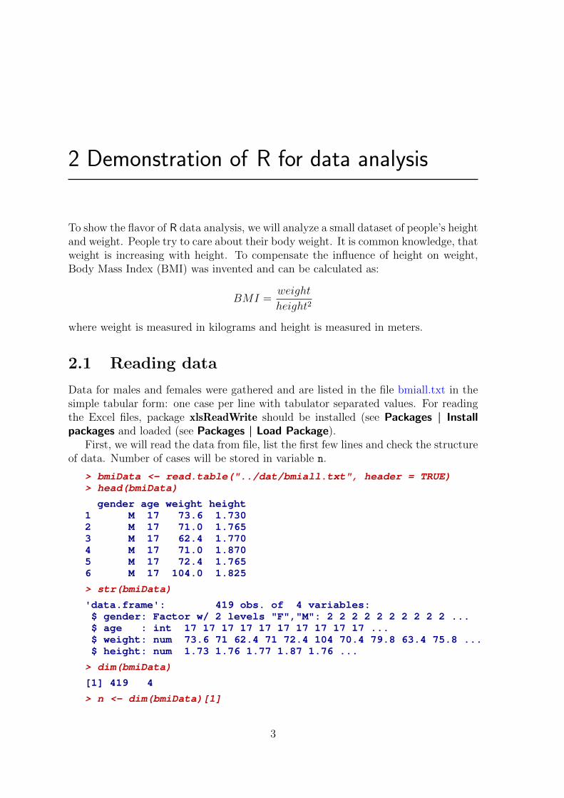
Data for males and females were gathered and are listed in the file bmiall.txt in thesimple tabular form: one case per line with tabulator separated values. For readingthe Excel files, package xlsReadWrite should be installed (see Packages | Installpackages and loaded (see Packages | Load Package).
First, we will read the data from file, list the first few lines and check the structureof data. Number of cases will be stored in variable n.
> bmiData <- read.table("../dat/bmiall.txt", header = TRUE)> head(bmiData)
gender age weight height1 M 17 73.6 1.7302 M 17 71.0 1.7653 M 17 62.4 1.7704 M 17 71.0 1.8705 M 17 72.4 1.7656 M 17 104.0 1.825
> str(bmiData)
'data.frame': 419 obs. of 4 variables:$ gender: Factor w/ 2 levels "F","M": 2 2 2 2 2 2 2 2 2 2 ...$ age : int 17 17 17 17 17 17 17 17 17 17 ...$ weight: num 73.6 71 62.4 71 72.4 104 70.4 79.8 63.4 75.8 ...$ height: num 1.73 1.76 1.77 1.87 1.76 ...
> dim(bmiData)
[1] 419 4
> n <- dim(bmiData)[1]
3
4 CHAPTER 2. DEMONSTRATION OF R FOR DATA ANALYSISVariables have different types, gender is descriptive, the rest are numeric. R
adapts the default (and possible) operations according to variable types:
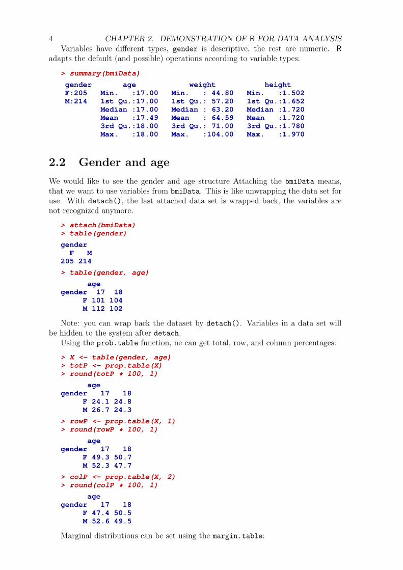
> summary(bmiData)
gender age weight heightF:205 Min. :17.00 Min. : 44.80 Min. :1.502M:214 1st Qu.:17.00 1st Qu.: 57.20 1st Qu.:1.652
Median :17.00 Median : 63.20 Median :1.720Mean :17.49 Mean : 64.59 Mean :1.7203rd Qu.:18.00 3rd Qu.: 71.00 3rd Qu.:1.780Max. :18.00 Max. :104.00 Max. :1.970
2.2 Gender and age
We would like to see the gender and age structure Attaching the bmiData means,that we want to use variables from bmiData. This is like unwrapping the data set foruse. With detach(), the last attached data set is wrapped back, the variables arenot recognized anymore.
> attach(bmiData)> table(gender)
genderF M
205 214
> table(gender, age)
agegender 17 18
F 101 104M 112 102
Note: you can wrap back the dataset by detach(). Variables in a data set willbe hidden to the system after detach.
Using the prob.table function, ne can get total, row, and column percentages:
> X <- table(gender, age)> totP <- prop.table(X)> round(totP * 100, 1)
agegender 17 18
F 24.1 24.8M 26.7 24.3
> rowP <- prop.table(X, 1)> round(rowP * 100, 1)
agegender 17 18
F 49.3 50.7M 52.3 47.7
> colP <- prop.table(X, 2)> round(colP * 100, 1)
agegender 17 18
F 47.4 50.5M 52.6 49.5
Marginal distributions can be set using the margin.table:

2.2. GENDER AND AGE 5Total number of cases
> margin.table(X)
[1] 419
and margins first by rows and then by columns
> margin.table(X, 1)
genderF M
205 214
> margin.table(X, 2)
age17 18213 206
Margins can be added to to the table
> Xm <- addmargins(X)> Xm
agegender 17 18 Sum
F 101 104 205M 112 102 214Sum 213 206 419
Although one can get marginal distributions with a function margin.table, wewill do it to demonstrate the powerful function apply. For brevity, we will define twoconstants byRow = 1 and byColumn = 2. They are saying, which index in a table touse for calculation of marginal sums.
> byRow <- 1> byColumn <- 2> (Rsum <- apply(X, byRow, sum))
F M205 214
> (Csum <- apply(X, byColumn, sum))
17 18213 206
> X/Rsum
agegender 17 18
F 0.4926829 0.5073171M 0.5233645 0.4766355
The first apply calculated the sum for each row, and the second one calculated thesum for each column. Don’t be confused with a strange-looking details in the code,try to grasp the general idea. apply is powerful way to say that some function hasto be applied to columns (2 in a call) or rows (1 in a call) of a table or matrix.
R is pretty smart in plotting. Objects carry class information, which helps R todecide how to plot the data. Beside the default plot, any other kind of plotting canbe prepared. Let us graphically present some tables.

6 CHAPTER 2. DEMONSTRATION OF R FOR DATA ANALYSISTo do this, let us look at the distribution in the heavier part of population i. e.
above the third quartile. First we calculate the third quartile and then prepare theselector variable. Then we use it to select cases, tabulate and plot.
> Q3 <- quantile(weight, 0.75)> select <- (weight > Q3)> X <- table(gender[select], age[select])> print(X)
17 18F 4 8M 43 49
> heading <- paste("Weight above Q3 = ", Q3)> plot(X, main = heading)
Weight above Q3 = 71
F M
1718
> barplot(X, beside = TRUE, col = c("pink", "lightblue"), main = heading)
17 18
Weight above Q3 = 71
010
2030
40
2.3. HEIGHT AND WEIGHT 7Both plots, the first one is known as mosaic plot, show that we have more males
in the heavy part.
2.3 Height and weight
Variables weight and height are numeric, which means that one can calculate varioussummary statistics:
> mean(weight)
[1] 64.5883
> mean(height)
[1] 1.719964
> sd(weight)
[1] 10.53051
> sd(height)
[1] 0.08752747
> (V <- var(cbind(weight, height)))
weight heightweight 110.8916572 0.601565848height 0.6015658 0.007661059
> cor(weight, height)
[1] 0.6526635
> my.cor <- V[1, 2]/(sd(weight) * sd(height))> cat("Correlation r =", my.cor, "\n")
Correlation r = 0.6526635
The last line shows one of the strengths of R : intermediate results are available forfurther calculation and printing! Correlation was calculated by taking the covarianceV[1,2] from the covariance matrix V and dividing by standard deviations calculatedby sd function. The cat concatenates and types the arguments; the argument "\n"
instructs it to go to next line.Are there differences in weight and height in gender age classes?
> aggregate(cbind(weight, height), list(age, gender), mean)
Group.1 Group.2 weight height1 17 F 58.51881 1.6506442 18 F 59.42500 1.6566443 17 M 69.12500 1.7758574 18 M 70.88137 1.791794
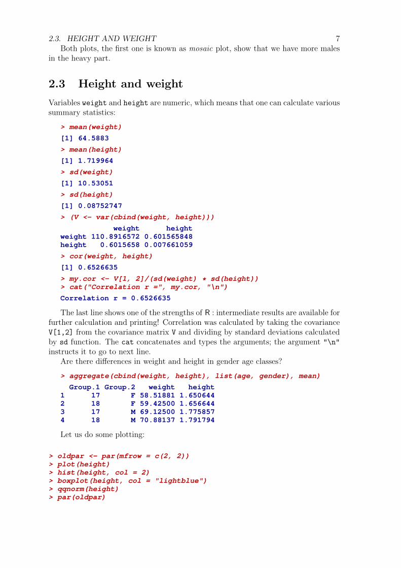
Let us do some plotting:
> oldpar <- par(mfrow = c(2, 2))> plot(height)> hist(height, col = 2)> boxplot(height, col = "lightblue")> qqnorm(height)> par(oldpar)
8 CHAPTER 2. DEMONSTRATION OF R FOR DATA ANALYSIS
●●●
●
●
●
●
●
●
●
●
●
●
●
●
●
●
●
●
●●
●
●
●
●
●●●●●●●
●
●●●
●
●
●●
●
●
●●
●●
●
●
●
●
●
●
●●
●
●●●
●
●●
●●
●●
●
●
●
●
●●
●
●
●
●●●
●
●
●●●
●
●
●●
●●
●●●
●●●
●
●
●
●
●●
●
●
●
●
●
●
●●
●
●●
●
●
●
●
●
●●
●
●
●
●
●
●
●
●
●●
●●
●
●
●
●●●●
●●●●
●●
●
●
●
●
●
●●●
●●●
●●
●●
●●
●
●
●
●
●●●
●
●
●
●●
●
●
●
●
●●
●
●
●
●
●●●
●●
●
●
●
●
●●
●●
●
●
●
●
●
●
●●●●●
●
●●●
●●●
●
●●
●
●
●
●
●
●
●
●●●
●●
●●●
●
●●
●●●●●●
●●
●
●
●
●●
●
●
●
●
●●
●
●
●
●
●●
●●
●
●
●
●
●
●●
●
●●
●
●●
●●●
●●●
●
●
●
●●
●●
●
●●●
●
●
●●●
●
●
●
●
●
●
●
●
●
●
●
●
●
●●
●
●
●
●●
●
●
●●
●●
●●●
●●
●
●
●●
●●●
●
●●
●●
●
●●
●
●●
●
●
●
●●●●
●●
●●
●●●
●●
●
●
●
●●
●●●
●
●●●●●●
●
●
●
●●
●
●
●●
●
●
●●●●
●
●
●
●●●
●
●●
●
●
●
●●●●
●●
●
●●
●
●●●●
●●
0 100 200 300 400
1.5
1.7
1.9
Index
heig
ht
Histogram of height
height
Fre
quen
cy
1.5 1.6 1.7 1.8 1.9 2.0
020
4060
80
1.5
1.7
1.9
●●●
●
●
●
●
●
●
●
●
●
●
●
●
●
●
●
●
●●
●
●
●
●
●●
●●●●●
●
●●
●
●
●
●●
●
●
●●
●●
●
●
●
●
●
●
●●
●
●●
●
●
●●
●●
●●
●
●
●
●
●●
●
●
●
●●
●
●
●
●●●
●
●
●●
●●
●●●
●●●
●
●
●
●
●●
●
●
●
●
●
●
●●
●
●●
●
●
●
●
●
●●
●
●
●
●
●
●
●
●
●●
●●
●
●
●
●●
●●
●●●●
●●
●
●
●
●
●
●●●
●●●
●●
●●
●●
●
●
●
●
●●●
●
●
●
●●
●
●
●
●
●●
●
●
●
●
●●●
●●
●
●
●
●
●●
●●
●
●
●
●
●
●
●●●●
●
●
●●●
●●●
●
●●
●
●
●
●
●
●
●
●●
●
●●
●●●
●
●●
●●●●
●●
●●
●
●
●
●●
●
●
●
●
●●
●
●
●
●
●●
●●
●
●
●
●
●
●●
●
●●
●
●●
●●●
●●
●
●
●
●
●●
●●
●
●●●
●
●
●●
●
●
●
●
●
●
●
●
●
●
●
●
●
●
●●
●
●
●
●●
●
●
●●
●●
●●●
●●
●
●
●●
●●●
●
●●
●●
●
●●
●
●●
●
●
●
●●●●
●●
●●
●●●
●●
●
●
●
●●
●●
●
●
●●●
●●●
●
●
●
●●
●
●
●●
●
●
●●●●
●
●
●
●●
●
●
●●
●
●
●
●●●●
●●
●
●●
●
●●●●
●●
−3 −2 −1 0 1 2 3
1.5
1.7
1.9
Normal Q−Q Plot
Theoretical Quantiles
Sam
ple
Qua
ntile
s
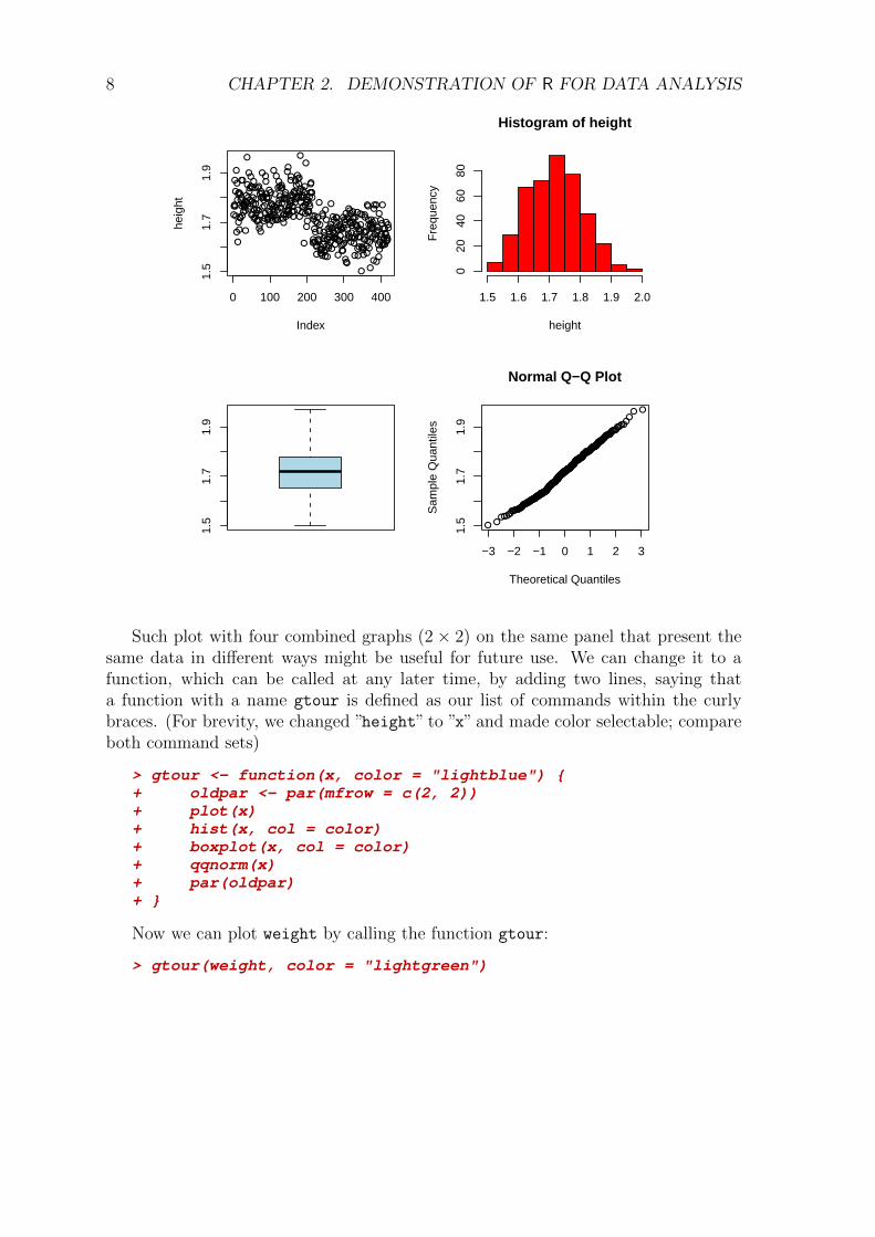
Such plot with four combined graphs (2× 2) on the same panel that present thesame data in different ways might be useful for future use. We can change it to afunction, which can be called at any later time, by adding two lines, saying thata function with a name gtour is defined as our list of commands within the curlybraces. (For brevity, we changed ”height” to ”x” and made color selectable; compareboth command sets)
> gtour <- function(x, color = "lightblue") {+ oldpar <- par(mfrow = c(2, 2))+ plot(x)+ hist(x, col = color)+ boxplot(x, col = color)+ qqnorm(x)+ par(oldpar)+ }
Now we can plot weight by calling the function gtour:
> gtour(weight, color = "lightgreen")
2.3. HEIGHT AND WEIGHT 9
●●
●
●●
●
●
●
●
●●
●
●
●
●
●
●
●
●
●●
●
●
●
●
●
●●
●
●
●
●
●
●
●●
●●●
●
●
●
●
●
●
●
●
●
●
●
●
●
●
●●
●●
●
●
●
●
●
●
●
●
●
●
●
●●●
●
●
●
●
●●
●
●
●
●
●
●
●●
●
●
●
●
●
●
●●
●
●
●●●
●
●
●
●
●
●
●
●
●●
●
●
●
●
●
●
●
●
●
●
●●
●
●
●
●
●
●
●
●
●●
●
●
●
●●
●
●
●
●
●
●
●
●
●
●●
●
●
●
●●
●
●
●●
●
●
●●
●●
●
●
●
●
●
●
●
●
●
●●●
●●
●
●
●
●●
●
●
●●
●●●
●
●
●●
●
●●●
●
●
●●●
●
●●
●●
●●
●
●
●●●
●
●●●
●
●
●
●●●●
●
●●●
●
●●●
●●
●
●
●●●●
●
●
●●
●
●
●
●
●
●●●●
●
●
●
●●
●●
●
●●
●●
●●
●
●
●
●●
●●
●
●●●
●
●
●●
●●
●●
●
●
●●
●
●
●●
●
●
●
●
●
●●
●
●
●●
●
●
●●
●●
●
●
●
●●●
●●●●●
●
●●●
●●
●●
●●
●
●●●
●
●
●
●●
●
●
●
●
●
●●
●
●
●
●
●●
●●
●
●●
●
●
●
●
●
●●
●●●
●
●
●
●●
●●
●
●●●●
●
●
●
●
●
●
●●●●
●
●
●●●
●
●●
●
●
●
●
●
●
●●
●●●●●
●
●●
●
●●●●
0 100 200 300 400
5070
90
Index
xHistogram of x
x
Fre
quen
cy
40 50 60 70 80 90
020
4060
80●
●●●●●●●●
5070
90
●●
●
●●
●
●
●
●
●●
●
●
●
●
●
●
●
●
●●
●
●
●
●
●
●●
●
●
●
●
●
●
●●
●●●
●
●
●
●
●
●
●
●
●
●
●
●
●
●
●●
●●
●
●
●
●
●
●
●
●
●
●
●
●●●
●
●
●
●
●●
●
●
●
●
●
●
●●
●
●
●
●
●
●
●●
●
●
●●●
●
●
●
●
●
●
●
●
●●
●
●
●
●
●
●
●
●
●
●
●●
●
●
●
●
●
●
●
●
●●
●
●
●
●●
●
●
●
●
●
●
●
●
●
●●
●
●
●
●●
●
●
●●
●
●
●●
●●
●
●
●
●
●
●
●
●
●
●●●
●●
●
●
●
●●
●
●
●●
●●
●
●
●
●●
●
●●●
●
●
●●
●
●
●●
●●
●●
●
●
●●
●
●
●●●
●
●
●
●●●●
●
●●●
●
●●●
●●
●
●
●●
●●
●
●
●●
●
●
●
●
●
●●●
●
●
●
●
●●
●●
●
●●
●●
●●
●
●
●
●●
●●
●
●●
●
●
●
●●
●●
●●
●
●
●●
●
●
●●
●
●
●
●
●
●●
●
●
●●
●
●
●●
●●
●
●
●
●●●
●●●
●●
●
●●●
●●
●●
●●
●
●●●
●
●
●
●●
●
●
●
●
●
●●
●
●
●
●
●●
●●
●
●●
●
●
●
●
●
●●
●●●
●
●
●
●●
●●
●
●●●●
●
●
●
●
●
●
●●
●●
●
●
●●●
●
●●
●
●
●
●
●
●
●●
●●●●●
●
●●
●
● ●●●
−3 −2 −1 0 1 2 3
5070
90
Normal Q−Q Plot
Theoretical Quantiles
Sam
ple
Qua
ntile
s
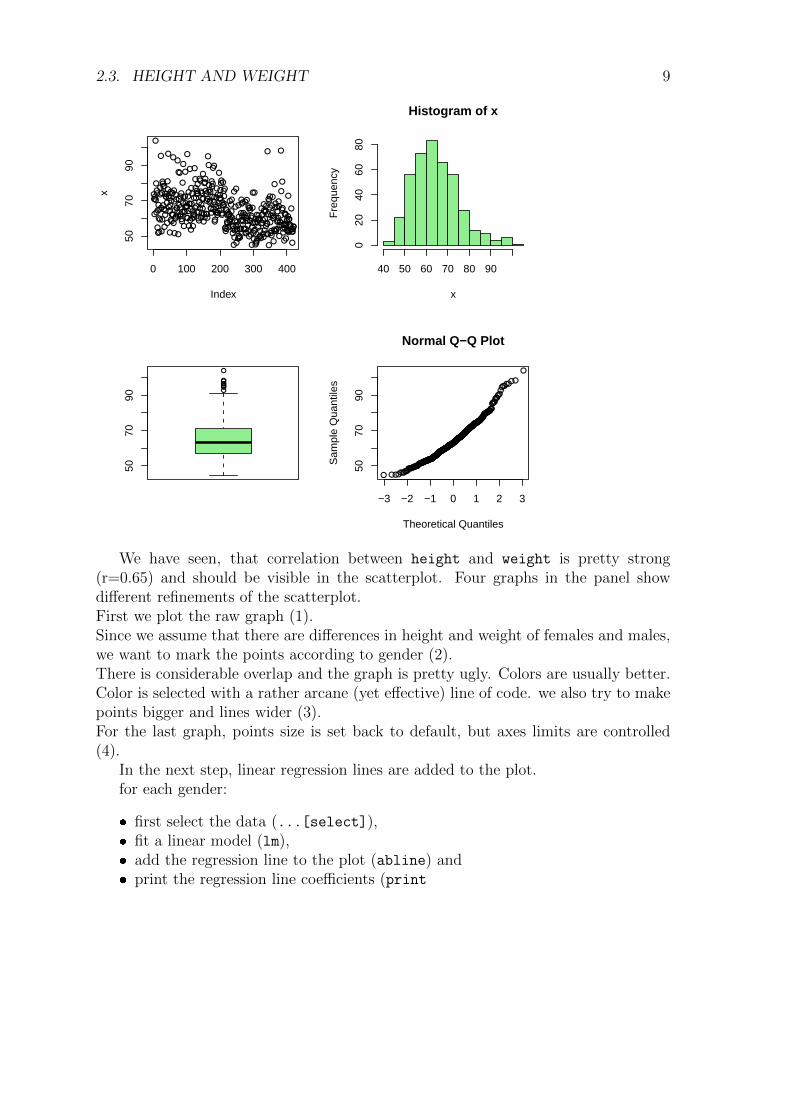
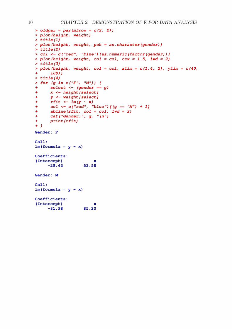
We have seen, that correlation between height and weight is pretty strong(r=0.65) and should be visible in the scatterplot. Four graphs in the panel showdifferent refinements of the scatterplot.First we plot the raw graph (1).Since we assume that there are differences in height and weight of females and males,we want to mark the points according to gender (2).There is considerable overlap and the graph is pretty ugly. Colors are usually better.Color is selected with a rather arcane (yet effective) line of code. we also try to makepoints bigger and lines wider (3).For the last graph, points size is set back to default, but axes limits are controlled(4).
In the next step, linear regression lines are added to the plot.for each gender:
� first select the data (...[select]),� fit a linear model (lm),� add the regression line to the plot (abline) and� print the regression line coefficients (print
10 CHAPTER 2. DEMONSTRATION OF R FOR DATA ANALYSIS
> oldpar = par(mfrow = c(2, 2))> plot(height, weight)> title(1)> plot(height, weight, pch = as.character(gender))> title(2)> col <- c("red", "blue")[as.numeric(factor(gender))]> plot(height, weight, col = col, cex = 1.5, lwd = 2)> title(3)> plot(height, weight, col = col, xlim = c(1.4, 2), ylim = c(40,+ 100))> title(4)> for (g in c("F", "M")) {+ select <- (gender == g)+ x <- height[select]+ y <- weight[select]+ rfit <- lm(y ~ x)+ col <- c("red", "blue")[(g == "M") + 1]+ abline(rfit, col = col, lwd = 2)+ cat("Gender:", g, "\n")+ print(rfit)+ }
Gender: F
Call:lm(formula = y ~ x)
Coefficients:(Intercept) x
-29.63 53.58
Gender: M
Call:lm(formula = y ~ x)
Coefficients:(Intercept) x
-81.98 85.20

2.4. INFERENCE 11
●●
●
●●
●
●
●
●
●●
●
●
●
●
●
●
●
●
●●
●
●
●
●
●
● ●
●
●
●
●
●
●
●●
●●●
●
●
●
●
●
●
●
●
●
●
●
●
●
●
●●
● ●
●
●
●
●
●
●
●
●
●
●
●
●●●
●
●
●
●
●●
●
●
●
●
●
●
●●
●
●
●
●
●
●
●●
●
●
●●●
●
●
●
●
●
●
●
●
● ●
●
●
●
●
●
●
●
●
●
●
●●
●
●
●
●
●
●
●
●
●●
●
●
●
●●
●
●
●
●
●
●
●
●
●
●●
●
●
●
●●
●
●
●●
●
●
●●
●●
●
●
●
●
●
●
●
●
●
●●●
●●
●
●
●
●●
●
●
●●
●●
●
●
●
●●
●
●●●
●
●
●●
●
●
●●
● ●
●●
●
●
●●●
●
●●●
●
●
●
●●● ●
●
● ●●
●
●●●
●●
●
●
●●
●●
●
●
●●
●
●
●
●
●
●● ●
●
●
●
●
●●
●●
●
●●
●●
●●
●
●
●
●●
●●
●
●●
●
●
●
●●
●●
●●
●
●
●●
●
●
● ●
●
●
●
●
●
●●
●
●
●●
●
●
● ●
●●
●
●
●
● ●●
●●●
● ●
●
●●●
●●
● ●
●●
●
●● ●
●
●
●
●●
●
●
●
●
●
●●
●
●
●
●
●●
●●
●
● ●
●
●
●
●
●
●●
●● ●
●
●
●
● ●
●●
●
● ●●●
●
●
●
●
●
●
●●
●●
●
●
● ●●
●
●●
●
●
●
●
●
●
●●
●●●● ●
●
●●
●
●●●●
1.5 1.6 1.7 1.8 1.9
5070
90
height
wei
ght
1
M MM
MM
M
M
M
M
MM
M
M
M
MM
M
MM
MM
M
M
M
M
M
MM
M
M
M
M
M
M
MMMMM
M
M
MM
M
MM
MM
M
MM
M
M
MM
M M
M
M
M
MM
M
MM
M
M
MMMM
M
M
M
M
MM
M
MMM
M
M
MMM
M
M
M
M
MMMM
M
M MMM
M
M
M
MM
M
M
MM
M
MM
M
M
MM
M
MM
MM
M
M
M
M
MM
MM
MM
M
MM
MMM
M
M
M
MM
MM
M
M MM
M
M
MM
M
M
M MM
M
MM
M M
M
M
M
M
M
MM
MM
MM M
M MM
M
M
MM
M
M
MMM
MMM
M
MM
M
MMM
M
MM MM
M
MM
MMMM
M
MMM
MM
MFF
F
F
FFF
F FF
F FF
F
FFFF
FF
FFF
FF
F
F
FF
FF
F
F
F
FF FF
F
FF
FFF
FFF
FF F
FF
F
FF
FFFF
F
F FFF
F
FFFF
FF
F
FFF
FF
F F
F
F
FF
FF FF
F
FF
F
F
F F
FF
F
FF
F FF
FF FF FF
FFF
FFF F
FF
FFF F
F
F
FFF
F
F
FF
F
FF
F
FF
F
F F
FF
F
F F
FF
F
F
F
FF
FFF
FF
FFF
FF
FF FF
F
F
F
F
F
F
F
F FFF
FF
F FF
FF FFF
FF
F
FFF
F FFF F
F
FFFFF FF
1.5 1.6 1.7 1.8 1.9
5070
90
height
wei
ght
2
● ●
●
●●
●
●
●
●
●●
●
●
●
●
●
●
●●
●●
●
●
●
●
●
● ●
●
●
●
●
●
●
●●
●●●●
●
●●
●
●●
●
●
●
●
●
●
●
●●
● ●
●
●
●
●●
●
●●
●
●
●●●
●
●
●
●
●
●●
●
●●●
●
●
●●●
●
●
●
●
●
●●
●
●
● ●●●
●
●
●
●
●
●
●
●●
●
●●
●
●
●
●
●
●
●●●
●
●
●
●
●●
●●
●●
●
●●
●●
●
●
●
●
●●
●
●●
●●
●
●
●
●●
●
●
● ●
●
●
●●
● ●
●
●
●
●
●
●
●●
●
●● ●
●●
●
●
●
●●
●
●
●●
●●
●●
●
●●
●
●●●
●
●
● ●●
●
●●
●●
●●
●
●
●●●
●
●●●
●
●
●●●
● ●
●
●●●
●
●●●
●●
●
●●●
●●
●
●
●●
●
●
●
●
●
●● ●●
●
●●
●●●
●●●
●
● ●
●●
●
●●
●●
●●
●
●●●
●
●
●●
●●
●●
●
●
●●●
●
● ●
●
●
●
●
●●
●●
●
●●
●
●
● ●
●●
●
●●
● ●●
●●●
● ●
●
●●●
●●
● ●
●●
●●● ●
●
●
●●●
●
●
●
●
●
●●
●
●●
●
● ●
●●
●
●●
●●
●
●
●
●●
●●●
●
●●●●
●●
●● ●●
●
●
●
●
●
●
●
● ●●●
●
●
● ●●
●
● ●●●
●
●
●
●
●●●
●●● ●
●
●●●●●
●●
1.5 1.6 1.7 1.8 1.9
5070
90
height
wei
ght
3
●●
●
●●
●
●
●
●
●●
●
●
●
●
●
●
●
●
●●
●
●
●
●
●
● ●
●
●
●
●
●
●
●●
●●●
●
●
●
●
●
●
●
●
●
●
●
●
●
●
●●
● ●
●
●
●
●
●
●
●
●
●
●
●
●●●
●
●
●
●
●●
●
●
●
●
●
●
●●
●
●
●
●
●
●
●●
●
●
●●●
●
●
●
●
●
●
●
●
●●
●
●
●
●
●
●
●
●
●
●
●●
●
●
●
●
●
●
●
●
●●
●
●
●
●●
●
●
●
●
●
●
●
●
●
●●
●
●
●
●●
●
●
●●
●
●
●●
●●
●
●
●
●
●
●
●
●
●
●●●
●●
●
●
●
●●
●
●
●●
●●
●
●
●
●●
●
●●●
●
●
●●
●
●
●●
● ●
●●
●
●
●●●
●
●●●
●
●
●
●●● ●
●
● ●●
●
●●●
●●
●
●
●●
●●
●
●
●●
●
●
●
●
●
●● ●●
●
●
●
●●
●●
●
●●
●●
●●
●
●
●
●●
●●
●
●●
●
●
●
●●
●●
●●
●
●
●●
●
●
● ●
●
●
●
●
●
●●
●
●
●●
●
●
● ●
●●
●
●
●
● ●●
●●●
● ●
●
●●●
●●
● ●
●●
●
●● ●
●
●
●
●●
●
●
●
●
●
●●
●
●
●
●
●●
●●
●
● ●
●
●
●
●
●
●●
●●●
●
●
●
●●
●●
●
● ●●●
●
●
●
●
●
●
●●
●●
●
●
● ●●
●
●●
●
●
●
●
●
●
●●
●●●● ●
●
●●
●
●●●●
1.4 1.6 1.8 2.0
4060
8010
0
height
wei
ght
4
2.4 Inference
Are there any effects of gender and age on weight and height? We can test this byanalysis of variance:
> summary(aov(height ~ gender + age))
Df Sum Sq Mean Sq F value Pr(>F)gender 1 1.76308 1.76308 514.1828 < 2e-16 ***age 1 0.01282 0.01282 3.7395 0.05382 .Residuals 416 1.42642 0.00343---Signif. codes: 0 '***' 0.001 '**' 0.01 '*' 0.05 '.' 0.1 ' ' 1
> summary(aov(weight ~ gender + age))
Df Sum Sq Mean Sq F value Pr(>F)gender 1 12631 12631.2 156.6954 <2e-16 ***age 1 188 187.9 2.3305 0.1276Residuals 416 33534 80.6---Signif. codes: 0 '***' 0.001 '**' 0.01 '*' 0.05 '.' 0.1 ' ' 1
Or, since there is no influence of age, by t-test :

12 CHAPTER 2. DEMONSTRATION OF R FOR DATA ANALYSIS
> t.test(height ~ gender)
Welch Two Sample t-test
data: height by gendert = -22.6415, df = 416.359, p-value < 2.2e-16alternative hypothesis: true difference in means is not equal to 095 percent confidence interval:-0.1410314 -0.1184996sample estimates:mean in group F mean in group M
1.653688 1.783453
Sometimes functions return useful information, that can be used for further calcula-tions or used for informative comments:
> (tweight <- t.test(weight ~ gender))
Welch Two Sample t-test
data: weight by gendert = -12.5432, df = 410.525, p-value < 2.2e-16alternative hypothesis: true difference in means is not equal to 095 percent confidence interval:-12.70496 -9.26227sample estimates:mean in group F mean in group M
58.97854 69.96215
> names(tweight)
[1] "statistic" "parameter" "p.value" "conf.int" "estimate"[6] "null.value" "alternative" "method" "data.name"
> tweight$estimate
mean in group F mean in group M58.97854 69.96215
> cat("My comment about p-value (p =", tweight$p.value, ")\n")
My comment about p-value (p = 8.906156e-31 )

2.5. WHAT ABOUT THE BMI? 132.5 What about the BMI?
First, we calculate a new variable BMI and plot a gtour:
> BMI <- weight/(height^2)> gtour(BMI, col = "lightblue")
●
●
●●
●
●
●
●●●●
●●
●
●●
●
●●
●●
●
●
●
●
●
●●
●
●
●
●
●
●
●●
●
●
●
●
●
●●
●
●●●●
●
●●
●
●
●●
●●
●
●
●
●●
●
●
●●●
●
●
●●
●
●
●
●
●●
●
●●
●
●
●
●●●●
●
●
●
●
●●
●
●
●
●
●
●
●
●
●
●
●
●
●
●●
●
●●
●
●●
●●●
●●●●●
●
●
●●●
●●●
●
●●
●●●
●
●
●
●
●
●
●
●
●
●
●
●●
●
●
●
●
●
●
●
●
●●
●
●
●
●
●
●
●
●●●●
●●
●
●
●●●
●
●●
●
●
●●
●●●●
●
●
●
●
●
●●●
●
●
●
●
●
●●
●●
●●
●
●
●●●
●
●
●●
●
●
●
●
●●●●
●●
●
●●●●
●
●
●●●
●
●●
●
●
●
●●
●
●
●
●●
●
●
●
●
●
●
●●●●●●
●●
●●●●
●●
●●●
●
●
●●●●
●
●
●
●●
●●
●
●●●
●
●
●
●
●
●
●●
●●
●
●
●
●
●●●●
●
●●
●
●●●
●●
●
●●●
●
●
●●●●●●
●
●●
●
●●●●
●
●●
●
●
●
●
●
●
●
●
●●
●
●
●
●
●
●
●●●
●
●
●●
●●
●
●
●●
●●
●
●●
●●
●
●●
●
●
●
●
●
●
●
●
●
●●●
●
●
●
●
●
●
●●●
●
●
●●
●
●●
●●●●
●
●
●●
●
●●●●
0 100 200 300 400
2025
3035
Index
x
Histogram of x
x
Fre
quen
cy
20 25 30 35
040
8012
0
●
●●●●
●
●●●
2025
3035
●
●
●●
●
●
●
●●
●●
●●
●
●●
●
●●
●●
●
●
●
●
●
●●
●
●
●
●
●
●
●●
●
●
●
●
●
●●
●
●●
●●
●
●●
●
●
●●
●●
●
●
●
●●
●
●
●●
●
●
●
●●
●
●
●
●
●●
●
●●
●
●
●
●●
●●
●
●
●
●
●●
●
●
●
●
●
●
●
●
●
●
●
●
●
●●
●
●●
●
●●
●●
●
●●●●
●
●
●
●●●
●●●
●
●●
●●
●
●
●
●
●
●
●
●
●
●
●
●
●●
●
●
●
●
●
●
●
●
●●
●
●
●
●
●
●
●
●●●●
●●
●
●
●●●
●
●●
●
●
●●
●●●●
●
●
●
●
●
●●●
●
●
●
●
●
●●
●●
●●
●
●
●●●
●
●
●●
●
●
●
●
●●●●
●●
●
●●●●
●
●
●●
●
●
●●
●
●
●
●●
●
●
●
●●
●
●
●
●
●
●
●●
●●●
●
●●
●●●
●
●●
●●●
●
●
●●●●
●
●
●
●●
●●
●
●●
●
●
●
●
●
●
●
●●
●●
●
●
●
●
●●●
●
●
●●
●
●●
●
●●
●
●●●
●
●
●●●●●
●
●
●●
●
●●
●●
●
●●
●
●
●
●
●
●
●
●
●●
●
●
●
●
●
●
●●
●
●
●
●●
●●
●
●
●●
●●
●
●●
●●
●
●●
●
●
●
●
●
●
●
●
●
●●●
●
●
●
●
●
●
●●●
●
●
●●
●
●●
●●●●
●
●
●●
●
●●
●●
−3 −2 −1 0 1 2 3
2025
3035
Normal Q−Q Plot
Theoretical Quantiles
Sam
ple
Qua
ntile
s
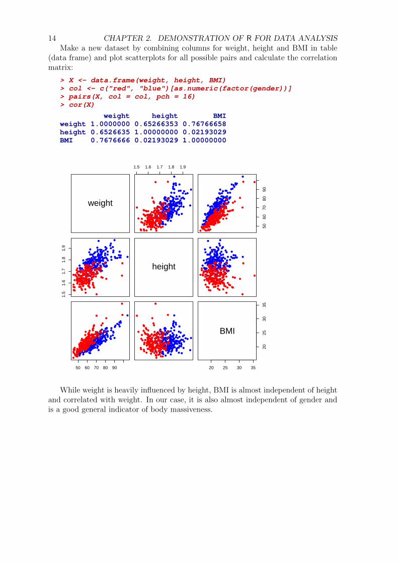
14 CHAPTER 2. DEMONSTRATION OF R FOR DATA ANALYSISMake a new dataset by combining columns for weight, height and BMI in table
(data frame) and plot scatterplots for all possible pairs and calculate the correlationmatrix:
> X <- data.frame(weight, height, BMI)> col <- c("red", "blue")[as.numeric(factor(gender))]> pairs(X, col = col, pch = 16)> cor(X)
weight height BMIweight 1.0000000 0.65266353 0.76766658height 0.6526635 1.00000000 0.02193029BMI 0.7676666 0.02193029 1.00000000
weight
1.5 1.6 1.7 1.8 1.9
●●
●
●●
●
●
●
●
●●
●
●
●
●
●
●
●
●
●
●
●
●
●
●
●
● ●
●
●
●
●
●
●
●●
●●●
●
●
●
●
●
●
●
●
●
●
●
●
●
●
●
●
● ●
●
●
●
●
●
●
●
●
●
●
●
●●●
●
●
●
●
●●
●
●
●
●
●
●
●●
●
●
●
●
●
●
●●
●
●
●●●
●
●
●
●
●
●
●
●
● ●
●
●
●
●
●
●
●
●
●
●
●●
●
●
●
●
●
●
●
●
●●
●
●
●
●●
●
●
●
●
●
●
●
●
●
●●
●
●
●
●
●
●
●
●●
●
●
●
●
●●
●
●
●
●
●
●
●
●
●
●●●
●●
●
●
●
●
●
●
●
●●
●
●●
●
●
●●
●
●
●●
●
●
●●
●
●
●●
● ●
●●
●
●
●●
●
●
●●●
●
●
●
●●
●●
●
● ●
●
●
●●●
●
●
●
●
●
●
●●
●
●
●
●
●
●
●
●
●
●
● ●●
●
●
●
●●
●
●
●
●
●
●●
●●
●
●
●
●●
●●
●
●●
●
●
●
●●
●●
●●
●
●
●●
●
●
● ●
●
●
●
●
●
●●
●
●
●
●
●
●
● ●
●
●
●
●
●
●●●
●●●
● ●
●
●
●●
●●
●●
●●
●
●
● ●
●
●
●
●●
●
●
●
●
●
●
●
●
●
●
●
●●
●
●
●
●●
●
●
●
●
●
●●
●● ●
●
●
●
●●
●●
●
●●●
●
●
●
●
●
●
●
●●
●●
●
●
● ●●
●
●●
●
●
●
●
●
●
●●
●●●●
●
●
●●
●
●● ●●
5060
7080
90
●●
●
●●
●
●
●
●
●●
●
●
●
●
●
●
●
●
●
●
●
●
●
●
●
●●
●
●
●
●
●
●
●●
● ●●
●
●
●
●
●
●
●
●
●
●
●
●
●
●
●
●
●●
●
●
●
●
●
●
●
●
●
●
●
● ●●
●
●
●
●
●●
●
●
●
●
●
●
●●
●
●
●
●
●
●
●●
●
●
●● ●
●
●
●
●
●
●
●
●
●●
●
●
●
●
●
●
●
●
●
●
●●
●
●
●
●
●
●
●
●
●●
●
●
●
●●
●
●
●
●
●
●
●
●
●
●●
●
●
●
●
●
●
●
●●
●
●
●
●
●●
●
●
●
●
●
●
●
●
●
●●●
●●
●
●
●
●
●
●
●
●●
●
●●
●
●
● ●
●
●
●●
●
●
●●
●
●
●●
●●
●●
●
●
●●
●
●
● ●●
●
●
●
● ●
●●
●
●●
●
●
●●●
●
●
●
●
●
●
●●
●
●
●
●
●
●
●
●
●
●
●●●
●
●
●
● ●
●
●
●
●
●
●●
●●
●
●
●
●●
● ●
●
●●
●
●
●
●●
●●
●●
●
●
●●
●
●
●●
●
●
●
●
●
●●
●
●
●
●
●
●
●●
●
●
●
●
●
●●●
● ●●
●●
●
●
●●
●●
●●
●●
●
●
●●
●
●
●
● ●
●
●
●
●
●
●
●
●
●
●
●
●●
●
●
●
●●
●
●
●
●
●
●●
● ●●
●
●
●
●●
●●
●
●● ●
●
●
●
●
●
●
●
●●
●●
●
●
●● ●
●
●●
●
●
●
●
●
●
●●
●●● ●
●
●
●●
●
●●●●
1.5
1.6
1.7
1.8
1.9
●
●●
●
●
●
●
●
●
●
●
●
●
●
●
●
●
●
●
●●
●
●
●
●
●
●
●● ●●●
●
●
●
●
●
●
●●
●
●
●●
●●
●
●
●
●
●
●
●●
●
●
●
●
●
●●
●●
●●
●
●
●
●
●●
●
●
●
●●
●
●
●
● ●●
●
●
●●
●●
●●●
●● ●
●
●
●
●
● ●
●
●
●
●
●
●
●●
●
●●
●
●
●
●
●
●●
●
●
●
●
●
●
●
●
●●
●●
●
●
●
●●
●
●
●● ●●
● ●
●
●
●
●
●
●●
●
●● ●
●●
●●
●●
●
●
●
●
●●
●
●
●
●
●●
●
●
●
●
●●
●
●
●
●
●● ●
●●
●
●
●
●
●●
●
●
●
●
●
●
●
●
●●●
●
●
●
●
● ●
●●●
●
●●
●
●
●
●
●
●
●
●
●
●
●●
●●●
●
●●
●
●●
●●
●
●●
●
●
●
● ●
●
●
●
●
●
●
●
●
●
●
●
●
●●
●
●
●
●
●
●
●
●
●●
●
●●
●
●●
●●
●
●
●
●
●●
● ●
●
●
●●
●
●
●●
●
●
●
●
●
●
●
●
●
●
●
●
●
●
●●
●
●
●
●●
●
●
●●
●●
●
●●
●●
●
●
●
●
●
● ●
●
●
●
●
●
●
●●
●
●●
●
●
●
●● ●●
●
●
● ●
●
●●
●
●
●
●
●
●●
●●
●
●
●●●
●●●
●
●
●
●●
●
●
● ●
●
●
●●●
●
●
●
●
●
●●
●
● ●
●
●
●
● ●●●
●●
●
● ●
●
●●●●
●●
height ●
●●
●
●
●
●
●
●
●
●
●
●
●
●
●
●
●
●
●●
●
●
●
●
●
●
●● ●●●
●
●
●
●
●
●
●●
●
●
●●
●●
●
●
●
●
●
●
●●
●
●
●
●
●
●●
●●
●●
●
●
●
●
●●
●
●
●
●●
●
●
●
● ●●
●
●
●●
●●
●●●
●● ●
●
●
●
●
● ●
●
●
●
●
●
●
●●
●
●●
●
●
●
●
●
●●
●
●
●
●
●
●
●
●
●●
●●
●
●
●
●●
●
●
●● ●●
● ●
●
●
●
●
●
●●
●
●● ●
●●
●●
●●
●
●
●
●
●●
●
●
●
●
●●
●
●
●
●
●●
●
●
●
●
●● ●
●●
●
●
●
●
●●
●
●
●
●
●
●
●
●
●●●
●
●
●
●
● ●
●●●
●
●●
●
●
●
●
●
●
●
●
●
●
●●
●●●
●
●●
●
●●
●●
●
●●
●
●
●
● ●
●
●
●
●
●
●
●
●
●
●
●
●
●●
●
●
●
●
●
●
●
●
●●
●
●●
●
●●
●●
●
●
●
●
●●
● ●
●
●
●●
●
●
●●
●
●
●
●
●
●
●
●
●
●
●
●
●
●
●●
●
●
●
●●
●
●
●●
●●
●
●●
●●
●
●
●
●
●
● ●
●
●
●
●
●
●
●●
●
●●
●
●
●
●● ●●
●
●
● ●
●
●●
●
●
●
●
●
●●
●●
●
●
●●●
●●●
●
●
●
●●
●
●
● ●
●
●
●●●
●
●
●
●
●
●●
●
● ●
●
●
●
● ●●●
●●
●
● ●
●
●●●●
●●
50 60 70 80 90
●
●
● ●
●
●
●
●●
●
●
●
●
●
●●
●
●●
●
●
●
●
●
●
●
●
●
●
●
●
●
●
●
●
●
●
●
●
●
●
●●
●
●
●
●
●
●
●●
●
●
●●
●●
●
●
●
●●
●
●
●●
●
●
●
●
●
●
●
●
●
●
●
●
●●
●
●
●
●●
●
●
●
●
●
●
●●
●
●
●
●
●
●
●
●
●
●
●
●
●
●●
●
●
●
●
●●
●
●●
●
●● ●
●
●
●
●●●
● ●●
●
●●
●●
●
●
●
●
●
●
●
●
●
●
●
●
●●
●
●
●
●
●
●
●
●
●●
●
●
●
●
●
●
●
● ●● ●
●●
●
●
●●●
●
●●
●
●
●●
●● ● ●
●
●
●
●
●
●
● ●
●
●
●
●
●
●●
●●
●●
●
●
●●
●
●
●
●●
●
●
●
●
●●
●●
●●
●
●
●●●
●
●
●
●●
●
●●
●
●
●
●●
●
●
●
● ●
●
●
●
●
●
●
●
●●
● ●
●
●●
●●
●
●
● ●
●●●
●
●
●●●
●
●
●
●
●
●
●●
●
●●
●
●
●
●
●
●
●
●●
●●
●
●
●
●
●●
●●
●
●●
●
●●
●
●●
●
● ●●
●
●
●●●
●●
●
●
●●
●
●
●●
●
●
●
●
●
●
●
●
●
●
●
●
●
●
●
●
●
●
●
●
●
●
●
●
●
●●
●
●
●
●
●●
●●
●
●●
●●
●
●●
●
●
●
●
●
●
●
●
●
●●●
●
●
●
●
●
●
●●●
●
●
●●
●
●●
● ●●
●
●
●
●
●
●
●●●●
●
●
● ●
●
●
●
●●
●
●
●
●
●
●●
●
●●
●
●
●
●
●
●
●
●
●
●
●
●
●
●
●
●
●
●
●
●
●
●
●●
●
●
●
●
●
●
●●
●
●
●●
●●
●
●
●
●●
●
●
●●
●
●
●
●
●
●
●
●
●
●
●
●
●●
●
●
●
●●
●
●
●
●
●
●
●●
●
●
●
●
●
●
●
●
●
●
●
●
●
●●
●
●
●
●
●●
●
●●
●
●● ●
●
●
●
●●●
● ●●
●
●●
●●
●
●
●
●
●
●
●
●
●
●
●
●
●●
●
●
●
●
●
●
●
●
●●
●
●
●
●
●
●
●
● ●● ●
●●
●
●
●●●
●
●●
●
●
●●
●●● ●
●
●
●
●
●
●
● ●
●
●
●
●
●
●●
●●
●●
●
●
●●
●
●
●
●●
●
●
●
●
●●
●●
●●
●
●
●●●
●
●
●
●●
●
●●
●
●
●
●●
●
●
●
● ●
●
●
●
●
●
●
●
●●
● ●
●
●●
●●
●
●
● ●
●●●
●
●
● ●●
●
●
●
●
●
●
●●
●
●●
●
●
●
●
●
●
●
●●
●●
●
●
●
●
●●
●●
●
●●
●
●●
●
●●
●
● ●●
●
●
●●●
●●
●
●
●●
●
●
●●
●
●
●
●
●
●
●
●
●
●
●
●
●
●
●
●
●
●
●
●
●
●
●
●
●
●●
●
●
●
●
●●
●●
●
● ●
●●
●
● ●
●
●
●
●
●
●
●
●
●
●●●
●
●
●
●
●
●
●●●
●
●
●●
●
●●
● ●●
●
●
●
●
●
●
●●
●●
20 25 30 35
2025
3035
BMI
While weight is heavily influenced by height, BMI is almost independent of heightand correlated with weight. In our case, it is also almost independent of gender andis a good general indicator of body massiveness.
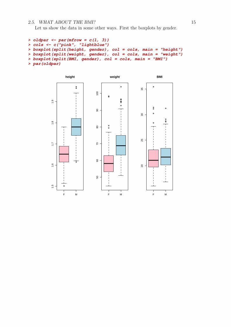
2.5. WHAT ABOUT THE BMI? 15Let us show the data in some other ways. First the boxplots by gender.
> oldpar <- par(mfrow = c(1, 3))> cols <- c("pink", "lightblue")> boxplot(split(height, gender), col = cols, main = "height")> boxplot(split(weight, gender), col = cols, main = "weight")> boxplot(split(BMI, gender), col = cols, main = "BMI")> par(oldpar)
●
●
●
●
F M
1.5
1.6
1.7
1.8
1.9
height
●
●
●
●
●
●
●
●
●
●
●
F M
5060
7080
9010
0
weight
●
●
●
●
●
●
●
●
●
F M
2025
3035
BMI

16 CHAPTER 2. DEMONSTRATION OF R FOR DATA ANALYSISOne can control the plotted symbols, their size can be calculated according to
some variable, in our case the BMI. (You can try other divisors beside 15)
> cols <- c("red", "blue")> pairs(X, cex = BMI/15, col = cols)
weight
1.5 1.6 1.7 1.8 1.9
●●
●
●●
●
●
●
●
●●
●
●
●
●
●
●
●
●
●●
●
●
●
●
●
●●
●
●
●
●
●
●
●●
●●●●
●
●●
●
●
●
●
●
●
●
●
●
●
●●
●●
●
●
●
●
●
●
●●
●
●
●●●
●
●
●
●
●
●●
●
●
●
●
●
●
●●
●
●
●
●
●
●
●●
●
●
●●●
●
●
●
●
●
●
●
●
●●
●
●
●
●
●
●
●
●
●
●
●●
●
●
●
●
●●
●●
●●
●
●●
●●
●
●
●
●
●
●
●
●●
●●
●
●
●
●●
●
●
● ●
●
●
●●
●●
●
●
●
●
●
●
●
●●
●●●
●●
●
●
●
●●
●
●
●●
●●
●
●
●
●●
●
●●●
●
●
● ●●
●
●●
● ●
●●
●
●
●●●
●
●●●
●
●
●
●●● ●
●
●●●
●
●●●
●●
●
●●●
●●
●
●
●●
●
●
●
●
●
●● ●●
●
●●
●●
●●
●●
●
● ●
●●
●
●●
●●
●●
●
●●●
●
●
●●
●●
●●
●
●
●●
●
●
● ●
●
●
●
●
●
●●
●
●
●●
●
●
● ●
●●
●
●
●
● ●●
●●●
● ●
●
●●●
●●
● ●
●●
●
●● ●
●
●
●
●●
●
●
●
●
●
●●
●
●
●
●
●●
●●
●
●●
●
●
●
●
●
●●
●●●
●
●
●
●●
●●
●
● ●●●
●
●
●
●
●
●
●●●●
●
●
● ●●
●
●●
●
●
●
●
●
●
●●
●●●● ●
●
●●
●
●●●●
5060
7080
90
●●
●
● ●
●
●
●
●
●●
●
●
●
●
●
●
●
●
●●
●
●
●
●
●
●●
●
●
●
●
●
●
●●
● ● ●●
●
●●
●
●
●
●
●
●
●
●
●
●
●●
●●
●
●
●
●
●
●
●●
●
●
●● ●
●
●
●
●
●
●●
●
●
●
●
●
●
●●
●
●
●
●
●
●
●●
●
●
●● ●
●
●
●
●
●
●
●
●
●●
●
●
●
●
●
●
●
●
●
●
●●
●
●
●
●
●●
●●
●●
●
●●
●●
●
●
●
●
●
●
●
●●
●●
●
●
●
●●
●
●
●●
●
●
●●
●●
●
●
●
●
●
●
●
●●
●●●
●●
●
●
●
●●
●
●
●●
●●●
●
●
● ●
●
●● ●
●
●
●●●
●
●●
●●
●●
●
●
●●
●
●
● ●●
●
●
●
● ●●●
●
●●●
●
●●●
●●
●
●●
●●●
●
●
●●
●
●
●
●
●
●●●●
●
●●
● ●
●●
●●
●
●●
●●
●
●●
●●
● ●
●
●●
●
●
●
●●
●●
●●
●
●
●●
●
●
●●
●
●
●
●
●
●●
●
●
●●
●
●
●●
●●
●
●
●
●●●
● ●●
●●
●
●●●
●●
●●
●●
●
●●●
●
●
●
● ●
●
●
●
●
●
●●
●
●
●
●
●●
●●
●
●●
●
●
●
●
●
●●
● ●●
●
●
●
●●
●●
●
●● ●●
●
●
●
●
●
●
●●
●●
●
●
●● ●
●
●●
●
●
●
●
●
●
●●
●●● ●●
●
● ●
●
●●●●
1.5
1.6
1.7
1.8
1.9
●●●
●
●
●
●
●
●
●
●
●
●
●
●
●
●
●
●
●●
●
●●
●
●
●●● ●●●
●
●●
●
●
●
●●
●
●
● ●●
●
●
●
●
●
●
●
●●
●
●●
●
●
●●
●●
●●
●
●●
●
●●
●
●
●
●●
●
●
●
● ●●
●
●
●●
●●
●●●
●● ●
●
●
●
●
● ●
●●
●
●
●
●
●●
●
●●
●
●
●
●
●
●●
●
●
●
●
●
●
●●
●●
●●
●
●
●
●●●
●
●● ●●
● ●
●
●
●
●
●
●●●
●● ●
●●
●●
●●
●
●
●
●
●●●
●
●
●
●●
●
●
●
●
●●
●
●
●
●
●● ●
●●
●
●●
●
●●
●●
●
●
●
●
●
●
●●●●
●●
●● ●
●●●
●
●●
●
●
●
●
●●
●
●●●
●●
●●●
●
●●
●●●●
●●
●●
●
●
●
● ●
●
●
●
●
●●
●
●
●
●
●●
●●
●
●
●
●
●
●●
●
●●
●
●●
●●●
●●
●
●●
●
●●
● ●
●
●●●
●
●
●●
●
●●
●
●
●
●
●
●
●
●
●
●
●
●●
●
●
●
●●
●
●
●●
● ●
●●●
●●
●
●
●●
●●●
●
●●
●●
●
●●
●
●●
●
●
●
●● ●●
●●
● ●
●●●
●●
●
●
●
●●
●●
●
●
●●●
●●●
●●
●
● ●
●
●
● ●
●
●
●●●●
●
●
●
●●
●
●
● ●
●
●
●
● ●●●
●●
●
● ●
●
●●●●
●●
height ●●●
●
●
●
●
●
●
●
●
●
●
●
●
●
●
●
●
●●
●
●●
●
●
●●● ●●●
●
●●
●
●
●
●●
●
●
● ●●
●
●
●
●
●
●
●
●●
●
●●
●
●
●●
●●
●●
●
●●
●
●●
●
●
●
●●
●
●
●
● ●●
●
●
●●
●●
●●●
●● ●
●
●
●
●
● ●
●●
●
●
●
●
●●
●
●●
●
●
●
●
●
●●
●
●
●
●
●
●
●●
●●
●●
●
●
●
●●●
●
●● ●●
● ●
●
●
●
●
●
●●●
●● ●
●●
●●
●●
●
●
●
●
●●●
●
●
●
●●
●
●
●
●
●●
●
●
●
●
●● ●
●●
●
●●
●
●●
●●
●
●
●
●
●
●
●●●●
●●
●● ●
●●●
●
●●
●
●
●
●
●●
●
●●
●
●●
●●●
●
●●
●●● ●
●●
●●
●
●
●
● ●
●
●
●
●
●●
●
●
●
●
●●
●●
●
●
●
●
●
●●
●
●●
●
●●
●●●
●●
●
●●
●
●●
● ●
●
●●●
●
●
●●
●
●●
●
●
●
●
●
●
●
●
●
●
●
●●
●
●
●
●●
●
●
●●
● ●
●●●
●●
●
●
●●
●●●
●
●●
●●
●
●●
●
●●
●
●
●
●● ●●
●●
● ●
●●●
●●
●
●
●
●●
●●
●
●
●●●
●●●
●●
●
● ●
●
●
● ●
●
●
●●●●
●
●
●
●●
●
●
● ●
●
●
●
● ●●●
●●
●
● ●
●
●●●●
●●
50 60 70 80 90
●●
● ●
●
●
●●
●●
●
●●
●
●●
●
●●
●●
●
●
●
●
●
●●
●
●
●
●
●
●
●●
●
●
●
●
●
●●
●
●●
●●
●
●●
●
●
●●
●●
●
●
●
●●
●
●●
●●
●
●
●●
●
●
●
●
●●
●
●●
●
●
●
●●
●●
●
●
●
●
●●
●
●
●
●
●
●
●
●
●
●
●
●
●
●●
●
●●
●
●●
●●
●
●●●
●●
●
●
●●●● ●●
●
●●
●●
●
●
●
●
●
●
●
●
●
●
●
●●●
●
●
●
●
●●
●
●
●●
●●
●
●
●
●
●
● ●● ●●●
●
●
●●●
●
●●
●●
●●
●●● ●
●
●
●●
●
●● ●
●
●
●
●
●
●●
●●
●●
●
●
●●●
●
●
●●
●●
●
●
● ●●●
●●
●
●●●●
●
●●
●●
●
●●
●
●
●
●●
●
●
●
● ●
●
●
●
●
●
●
●
●●
● ●●
● ●
●●●
●
● ●●●
●
●
●
●●●●
●
●
●
●●
●●
●
●●●
●
●
●●
●
●
●●
●●
●
●
●
●
●●●
●
●
●●
●
●●
●
●●
●
●●●
●
●
●●●●●
●
●
●●
●
●●●●
●
●●
●
●
●
●
●
●
●
●●
●
●
●
●
●
●
●
●●
●
●
●
● ●
●●
●
●
●●
●●
●
●●
●●
●
●●
●
●
●
●
●
●
●
●
●
●●●
●
●
●
●
●
●
●●●
●
●
● ●
●
●●
●●●●
●
●
●●
●
●●●●
●●
● ●
●
●
●●
●●
●
●●
●
●●
●
●●
●●
●
●
●
●
●
●●
●
●
●
●
●
●
●●
●
●
●
●
●
●●
●
●●
●●
●
●●
●
●
●●
●●
●
●
●
●●
●
●●
●●
●
●
●●
●
●
●
●
●●
●
●●
●
●
●
●●
●●
●
●
●
●
●●
●
●
●
●
●
●
●
●
●
●
●
●
●
●●
●
●●
●
●●
●●
●
●●● ●
●
●
●
●●●● ●●
●
●●
●●
●
●
●
●
●
●
●
●
●
●
●
●●●
●
●
●
●
●●
●
●
●●
●●
●
●
●
●
●
● ●● ●●●
●
●
●●●
●
●●
●●
●●
●●● ●
●
●
●●
●
●● ●
●
●
●
●
●
●●
●●
●●
●
●
●●●
●
●
●●
●●
●
●
● ● ●●
●●
●
●●●●
●
●●
●●
●
●●
●
●
●
●●
●
●
●
● ●
●
●
●
●
●
●
●
●●
● ●●
● ●
●●●
●
● ●●●
●
●
●
● ●●●
●
●
●
●●
●●
●
●●
●
●
●
●●
●
●
●●
●●
●
●
●
●
●●●
●
●
●●
●
●●
●
●●
●
● ●●
●
●
●●●●●
●
●
●●
●
●●
●●
●
●●
●
●
●
●
●
●
●
●●
●
●
●
●
●
●
●
●●
●
●
●
● ●
●●
●
●
●●
●●
●
●●
●●
●
● ●
●
●
●
●
●
●
●
●
●
●●●
●
●
●
●
●
●
●●●
●
●
● ●
●
●●
● ●●●
●
●
●●
●
●●
●●
20 25 30 35
2025
3035
BMI
According to the health tables, BMI classes are defined. We will cut the BMI intoclasses, rename the classes and order the levels of the factor bmic. Then we will plotprint and plot the table of coded BMI values.
> bmic <- cut(BMI, c(0, 13, 18, 25, 30, Inf))> levels(bmic)
[1] "(0,13]" "(13,18]" "(18,25]" "(25,30]" "(30,Inf]"
> levels(bmic) <- c("S", "s", "N", "h", "H")> bmic <- factor(bmic, levels = c("S", "s", "N", "h", "H"), ordered = T)> is.ordered(bmic)
[1] TRUE
Plotting the scatterplot with coded BMI as color and size of points, we can seethat BMI is a sort of principal component. The levels of BMI are running parallel tothe main variation line.
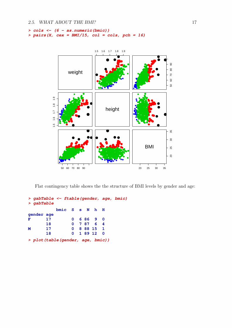
2.5. WHAT ABOUT THE BMI? 17
> cols <- (6 - as.numeric(bmic))> pairs(X, cex = BMI/15, col = cols, pch = 16)
weight
1.5 1.6 1.7 1.8 1.9
●●
●
●●
●
●
●
●
●●
●
●
●
●
●
●
●
●
●●
●
●
●
●
●
●●
●
●
●
●
●
●
●●
●●●●
●
●●
●
●
●
●
●
●
●
●
●
●
●●
●●
●
●
●
●
●
●
●●
●
●
●●●
●
●
●
●
●
●●
●
●
●
●
●
●
●●
●
●
●
●
●
●
●●
●
●
●●●
●
●
●
●
●
●
●
●
●●
●
●
●
●
●
●
●
●
●
●
●●
●
●
●
●
●●
●●
●●
●
●●
●●
●
●
●
●
●
●
●
●●
●●
●
●
●
●●
●
●
● ●
●
●
●●
●●
●
●
●
●
●
●
●
●●
●●●
●●
●
●
●
●●
●
●
●●
●●
●
●
●
●●
●
●●●
●
●
● ●●
●
●●
● ●
●●
●
●
●●●
●
●●●
●
●
●
●●● ●
●
●●●
●
●●●
●●
●
●●●
●●
●
●
●●
●
●
●
●
●
●● ●●
●
●●
●●
●●
●●
●
● ●
●●
●
●●
●●
●●
●
●●●
●
●
●●
●●
●●
●
●
●●
●
●
● ●
●
●
●
●
●
●●
●
●
●●
●
●
● ●
●●
●
●
●
● ●●
●●●
● ●
●
●●●
●●
● ●
●●
●
●● ●
●
●
●
●●
●
●
●
●
●
●●
●
●
●
●
●●
●●
●
●●
●
●
●
●
●
●●
●●●
●
●
●
●●
●●
●
● ●●●
●
●
●
●
●
●
●●●●
●
●
● ●●
●
●●
●
●
●
●
●
●
●●
●●●● ●
●
●●
●
●●●●
5060
7080
90
●●
●
● ●
●
●
●
●
●●
●
●
●
●
●
●
●
●
●●
●
●
●
●
●
●●
●
●
●
●
●
●
●●
● ● ●●
●
●●
●
●
●
●
●
●
●
●
●
●
●●
●●
●
●
●
●
●
●
●●
●
●
●● ●
●
●
●
●
●
●●
●
●
●
●
●
●
●●
●
●
●
●
●
●
●●
●
●
●● ●
●
●
●
●
●
●
●
●
●●
●
●
●
●
●
●
●
●
●
●
●●
●
●
●
●
●●
●●
●●
●
●●
●●
●
●
●
●
●
●
●
●●
●●
●
●
●
●●
●
●
●●
●
●
●●
●●
●
●
●
●
●
●
●
●●
●●●
●●
●
●
●
●●
●
●
●●
●●●
●
●
● ●
●
●● ●
●
●
●●●
●
●●
●●
●●
●
●
●●
●
●
● ●●
●
●
●
● ●●●
●
●●●
●
●●●
●●
●
●●
●●●
●
●
●●
●
●
●
●
●
●●●●
●
●●
● ●
●●
●●
●
●●
●●
●
●●
●●
● ●
●
●●
●
●
●
●●
●●
●●
●
●
●●
●
●
●●
●
●
●
●
●
●●
●
●
●●
●
●
●●
●●
●
●
●
●●●
● ●●
●●
●
●●●
●●
●●
●●
●
●●●
●
●
●
● ●
●
●
●
●
●
●●
●
●
●
●
●●
●●
●
●●
●
●
●
●
●
●●
● ●●
●
●
●
●●
●●
●
●● ●●
●
●
●
●
●
●
●●
●●
●
●
●● ●
●
●●
●
●
●
●
●
●
●●
●●● ●●
●
● ●
●
●●●●
1.5
1.6
1.7
1.8
1.9
●●●
●
●
●
●
●
●
●
●
●
●
●
●
●
●
●
●
●●
●
●●
●
●
●●● ●●●
●
●●
●
●
●
●●
●
●
● ●●
●
●
●
●
●
●
●
●●
●
●●
●
●
●●
●●
●●
●
●●
●
●●
●
●
●
●●
●
●
●
● ●●
●
●
●●
●●
●●●
●● ●
●
●
●
●
● ●
●●
●
●
●
●
●●
●
●●
●
●
●
●
●
●●
●
●
●
●
●
●
●●
●●
●●
●
●
●
●●●
●
●● ●●
● ●
●
●
●
●
●
●●●
●● ●
●●
●●
●●
●
●
●
●
●●●
●
●
●
●●
●
●
●
●
●●
●
●
●
●
●● ●
●●
●
●●
●
●●
●●
●
●
●
●
●
●
●●●●
●●
●● ●
●●●
●
●●
●
●
●
●
●●
●
●●●
●●
●●●
●
●●
●●●●
●●
●●
●
●
●
● ●
●
●
●
●
●●
●
●
●
●
●●
●●
●
●
●
●
●
●●
●
●●
●
●●
●●●
●●
●
●●
●
●●
● ●
●
●●●
●
●
●●
●
●●
●
●
●
●
●
●
●
●
●
●
●
●●
●
●
●
●●
●
●
●●
● ●
●●●
●●
●
●
●●
●●●
●
●●
●●
●
●●
●
●●
●
●
●
●● ●●
●●
● ●
●●●
●●
●
●
●
●●
●●
●
●
●●●
●●●
●●
●
● ●
●
●
● ●
●
●
●●●●
●
●
●
●●
●
●
● ●
●
●
●
● ●●●
●●
●
● ●
●
●●●●
●●
height ●●●
●
●
●
●
●
●
●
●
●
●
●
●
●
●
●
●
●●
●
●●
●
●
●●● ●●●
●
●●
●
●
●
●●
●
●
● ●●
●
●
●
●
●
●
●
●●
●
●●
●
●
●●
●●
●●
●
●●
●
●●
●
●
●
●●
●
●
●
● ●●
●
●
●●
●●
●●●
●● ●
●
●
●
●
● ●
●●
●
●
●
●
●●
●
●●
●
●
●
●
●
●●
●
●
●
●
●
●
●●
●●
●●
●
●
●
●●●
●
●● ●●
● ●
●
●
●
●
●
●●●
●● ●
●●
●●
●●
●
●
●
●
●●●
●
●
●
●●
●
●
●
●
●●
●
●
●
●
●● ●
●●
●
●●
●
●●
●●
●
●
●
●
●
●
●●●●
●●
●● ●
●●●
●
●●
●
●
●
●
●●
●
●●
●
●●
●●●
●
●●
●●● ●
●●
●●
●
●
●
● ●
●
●
●
●
●●
●
●
●
●
●●
●●
●
●
●
●
●
●●
●
●●
●
●●
●●●
●●
●
●●
●
●●
● ●
●
●●●
●
●
●●
●
●●
●
●
●
●
●
●
●
●
●
●
●
●●
●
●
●
●●
●
●
●●
● ●
●●●
●●
●
●
●●
●●●
●
●●
●●
●
●●
●
●●
●
●
●
●● ●●
●●
● ●
●●●
●●
●
●
●
●●
●●
●
●
●●●
●●●
●●
●
● ●
●
●
● ●
●
●
●●●●
●
●
●
●●
●
●
● ●
●
●
●
● ●●●
●●
●
● ●
●
●●●●
●●
50 60 70 80 90
●●
● ●
●
●
●●
●●
●
●●
●
●●
●
●●
●●
●
●
●
●
●
●●
●
●
●
●
●
●
●●
●
●
●
●
●
●●
●
●●
●●
●
●●
●
●
●●
●●
●
●
●
●●
●
●●
●●
●
●
●●
●
●
●
●
●●
●
●●
●
●
●
●●
●●
●
●
●
●
●●
●
●
●
●
●
●
●
●
●
●
●
●
●
●●
●
●●
●
●●
●●
●
●●●
●●
●
●
●●●● ●●
●
●●
●●
●
●
●
●
●
●
●
●
●
●
●
●●●
●
●
●
●
●●
●
●
●●
●●
●
●
●
●
●
● ●● ●●●
●
●
●●●
●
●●
●●
●●
●●● ●
●
●
●●
●
●● ●
●
●
●
●
●
●●
●●
●●
●
●
●●●
●
●
●●
●●
●
●
● ●●●
●●
●
●●●●
●
●●
●●
●
●●
●
●
●
●●
●
●
●
● ●
●
●
●
●
●
●
●
●●
● ●●
● ●
●●●
●
● ●●●
●
●
●
●●●●
●
●
●
●●
●●
●
●●●
●
●
●●
●
●
●●
●●
●
●
●
●
●●●
●
●
●●
●
●●
●
●●
●
●●●
●
●
●●●●●
●
●
●●
●
●●●●
●
●●
●
●
●
●
●
●
●
●●
●
●
●
●
●
●
●
●●
●
●
●
● ●
●●
●
●
●●
●●
●
●●
●●
●
●●
●
●
●
●
●
●
●
●
●
●●●
●
●
●
●
●
●
●●●
●
●
● ●
●
●●
●●●●
●
●
●●
●
●●●●
●●
● ●
●
●
●●
●●
●
●●
●
●●
●
●●
●●
●
●
●
●
●
●●
●
●
●
●
●
●
●●
●
●
●
●
●
●●
●
●●
●●
●
●●
●
●
●●
●●
●
●
●
●●
●
●●
●●
●
●
●●
●
●
●
●
●●
●
●●
●
●
●
●●
●●
●
●
●
●
●●
●
●
●
●
●
●
●
●
●
●
●
●
●
●●
●
●●
●
●●
●●
●
●●● ●
●
●
●
●●●● ●●
●
●●
●●
●
●
●
●
●
●
●
●
●
●
●
●●●
●
●
●
●
●●
●
●
●●
●●
●
●
●
●
●
● ●● ●●●
●
●
●●●
●
●●
●●
●●
●●● ●
●
●
●●
●
●● ●
●
●
●
●
●
●●
●●
●●
●
●
●●●
●
●
●●
●●
●
●
● ● ●●
●●
●
●●●●
●
●●
●●
●
●●
●
●
●
●●
●
●
●
● ●
●
●
●
●
●
●
●
●●
● ●●
● ●
●●●
●
● ●●●
●
●
●
● ●●●
●
●
●
●●
●●
●
●●
●
●
●
●●
●
●
●●
●●
●
●
●
●
●●●
●
●
●●
●
●●
●
●●
●
● ●●
●
●
●●●●●
●
●
●●
●
●●
●●
●
●●
●
●
●
●
●
●
●
●●
●
●
●
●
●
●
●
●●
●
●
●
● ●
●●
●
●
●●
●●
●
●●
●●
●
● ●
●
●
●
●
●
●
●
●
●
●●●
●
●
●
●
●
●
●●●
●
●
● ●
●
●●
● ●●●
●
●
●●
●
●●
●●
20 25 30 3520
2530
35
BMI
Flat contingency table shows the the structure of BMI levels by gender and age:
> gabTable <- ftable(gender, age, bmic)> gabTable
bmic S s N h Hgender ageF 17 0 6 86 9 0
18 0 7 87 6 4M 17 0 8 88 15 1
18 0 1 89 12 0
> plot(table(gender, age, bmic))

18 CHAPTER 2. DEMONSTRATION OF R FOR DATA ANALYSIS
table(gender, age, bmic)
gender
age
F M
1718
S s N h H S s N h H
A more common plot of BMI by gender would be
> barplot(table(gender, bmic), beside = TRUE, legend = TRUE)

2.5. WHAT ABOUT THE BMI? 19
S s N h H
FM
050
100
150

20 CHAPTER 2. DEMONSTRATION OF R FOR DATA ANALYSIS

3 How to start
3.1 Installation
Installation of R for Windows users is pretty straightforward. Download the latestsetup file (like R-2.7.1-win32.exe for version 2.7.1) from the base directory on thenearest CRAN site http://www.r-project.org, click on its icon to start installation,and follow instructions. Packages that do not come with the base distribution mustbe downloaded and installed separately. For more details. see the README file thatis included with the R distribution.
3.2 Invoking R
R can be started in any of the usual ways for starting programs under Windows. WhenR is started, it opens a canvas (named RGui ) which will hold the command window(R console ) and graphics windows (R graphics ). Initially it opens the commandwindow, graphics windows are opened on demand.
Figure 3.1 shows the R canvas with the command window. A simple command(2+2) giving the result 4 was given to R . Commands are preceded with a commandprompt character > and typed in red. Commands can span more than one line,in which case command continuation lines are marked with + . Several commands,separated by a semicolon (; ), can be typed in one line. Results are printed in blue.Some results are preceded with a number in square brackets (in our case [1]), whichshows the position of the next value in a list. This will be more obvious in longerprints. Hash (#) is a comment character: anything after the # is a comment and isignored by parser.
Commands can be literally typed in or pasted from clipboard. The Copy-Pastetechnique is very productive and can be used in connection with any text editor orword processing software. Certainly some editors are more suited for R than others (e. g. Rwinedt).
A very effective menu option Edit | Paste commands only (only available onWindows platform) is able to filter out any commands that are copied to clipboard(and mixed with any other text) and paste just commands (lines preceded with > and+) to the command window. One can select any portion of text in a .pdf file andpaste it to R . For example, you can copy lines from this paragraph to the end of thenext one, and use Paste commands only to get the result shown in the example.
21
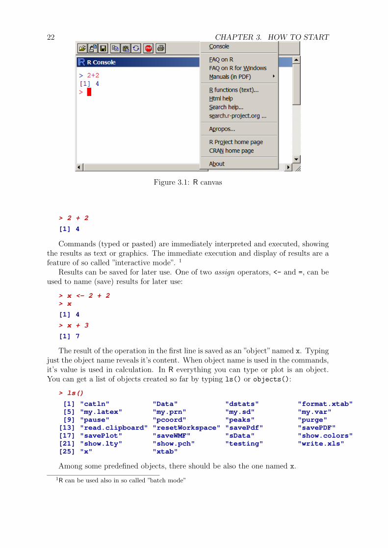
22 CHAPTER 3. HOW TO START
Figure 3.1: R canvas
> 2 + 2
[1] 4
Commands (typed or pasted) are immediately interpreted and executed, showingthe results as text or graphics. The immediate execution and display of results are afeature of so called ”interactive mode”. 1
Results can be saved for later use. One of two assign operators, <- and =, can beused to name (save) results for later use:
> x <- 2 + 2> x
[1] 4
> x + 3
[1] 7
The result of the operation in the first line is saved as an ”object”named x. Typingjust the object name reveals it’s content. When object name is used in the commands,it’s value is used in calculation. In R everything you can type or plot is an object.You can get a list of objects created so far by typing ls() or objects():
> ls()
[1] "catln" "Data" "dstats" "format.xtab"[5] "my.latex" "my.prn" "my.sd" "my.var"[9] "pause" "pcoord" "peaks" "purge"[13] "read.clipboard" "resetWorkspace" "savePdf" "savePDF"[17] "savePlot" "saveWMF" "sData" "show.colors"[21] "show.lty" "show.pch" "testing" "write.xls"[25] "x" "xtab"
Among some predefined objects, there should be also the one named x.
1R can be used also in so called ”batch mode”
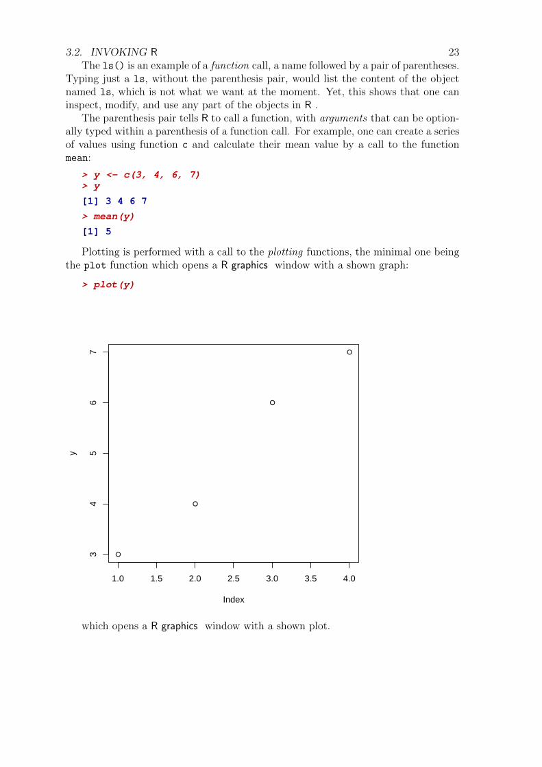
3.2. INVOKING R 23The ls() is an example of a function call, a name followed by a pair of parentheses.
Typing just a ls, without the parenthesis pair, would list the content of the objectnamed ls, which is not what we want at the moment. Yet, this shows that one caninspect, modify, and use any part of the objects in R .
The parenthesis pair tells R to call a function, with arguments that can be option-ally typed within a parenthesis of a function call. For example, one can create a seriesof values using function c and calculate their mean value by a call to the functionmean:
> y <- c(3, 4, 6, 7)> y
[1] 3 4 6 7
> mean(y)
[1] 5
Plotting is performed with a call to the plotting functions, the minimal one beingthe plot function which opens a R graphics window with a shown graph:
> plot(y)
●
●
●
●
1.0 1.5 2.0 2.5 3.0 3.5 4.0
34
56
7
Index
y
which opens a R graphics window with a shown plot.

24 CHAPTER 3. HOW TO START3.3 Workspace and History
All user created objects are stored in a memory space called workspace. All typed com-mands are saved into the history. You can view the history with a call history(100),which will show you the last 100 lines in a separate browser window. Workspace (andhistory) can be saved or loaded at any time by the use of menu commands File | Saveworkspace and File | Load workspace (File | Save history and File | Load historyrespectively). The images of the workspace and history are saved to disc when Rsession is closed. Saved workspace and history are loaded when you run R next time.
3.4 Working directory
It pays to create separate directory for every project and instruct R to use this di-rectory as a working directory. The working directory is then a default directory forall file manipulations, including saving and loading of the workspace, history or anyother files (e. g. data files). By default, R will start deep in the directory tree. Youcan check the working directory by getwd() and set a new one by setwd() or usingthe menu option (File | Change dir ...).
You can also exit R (File | Exit or type q()), save the workspace and history tothe project directory and restart R by double-clicking the icon for .Rimage in theproject directory. In this way, the previously saved workspace and history will bereloaded and working directory will be set to the project directory.
3.5 Packages
R is based on a number of packages. A package is basically a collection of functionsand other objects, accompanied with the standardized description and some usermanual (also called vignette ). A collection of basic packages are loaded when R isinvoked. Additional packages have to be first installed on your computer (Packages| Install packages ...) and then loaded to the workspace (Packages | Load package...). The collection of packages is growing so it is worth checking it from time to timefor the news. Packages are available Package section on CRAN web sites. Amongmany specialized packages, package hmisc (by Frank Harrell, miscellaneous functions)and MASS (Venables and Ripley, Modern Applied Statistics with S-PLUS) are prettyuseful.
3.6 Getting help
R provides many ways of getting help. Every function in supported packages has adescription page. This pages list function description, usage, arguments, returnedvalue, references, links to associated functions, and examples. To get the help onsome function, e. g. mean, one can type command help(mean) or simply ?mean .
In addition, Help (Figure 3.2) provides a series of help resources. First is a help
on Console (command window) shortcuts, like UpArrow ↑ and DownArrow ↓ , thatcan be used to scroll through previously typed commands and ← and → , that can

3.6. GETTING HELP 25
Figure 3.2: R Help menu
be used for correcting mistyped commands. A useful one might be CTRL-X, whichhas different meaning as usual: selected text in the console is pasted and eventuallyexecuted with a single keystroke. Tabulator key tab provides limited code completionof what you type and can be useful if you know just a beginning part of a function.If nothing happens, press the key twice to get a list of possible continuations.
Next you have a collection of FAQ and Manuals and entry to the individualfunctions help. Help | R functions (text)... is equivalent to function help whileHelp | Search help ... can be called via help.search:
> if (interactive()) {+ help(mean)+ help.search("mean")+ }
Html help is an entry to different local manual, a search engine and package descrip-tions and documentation.search R-project.org is a link to the R Site Search.Apropos (and function apropos("string")) lists all object names that include the”string”.
> apropos("mean")
[1] "colMeans" "kmeans" "mean" "mean.data.frame"[5] "mean.Date" "mean.default" "mean.difftime" "mean.POSIXct"[9] "mean.POSIXlt" "rowMeans" "weighted.mean"
With function example you can access Examples part of some functions like:
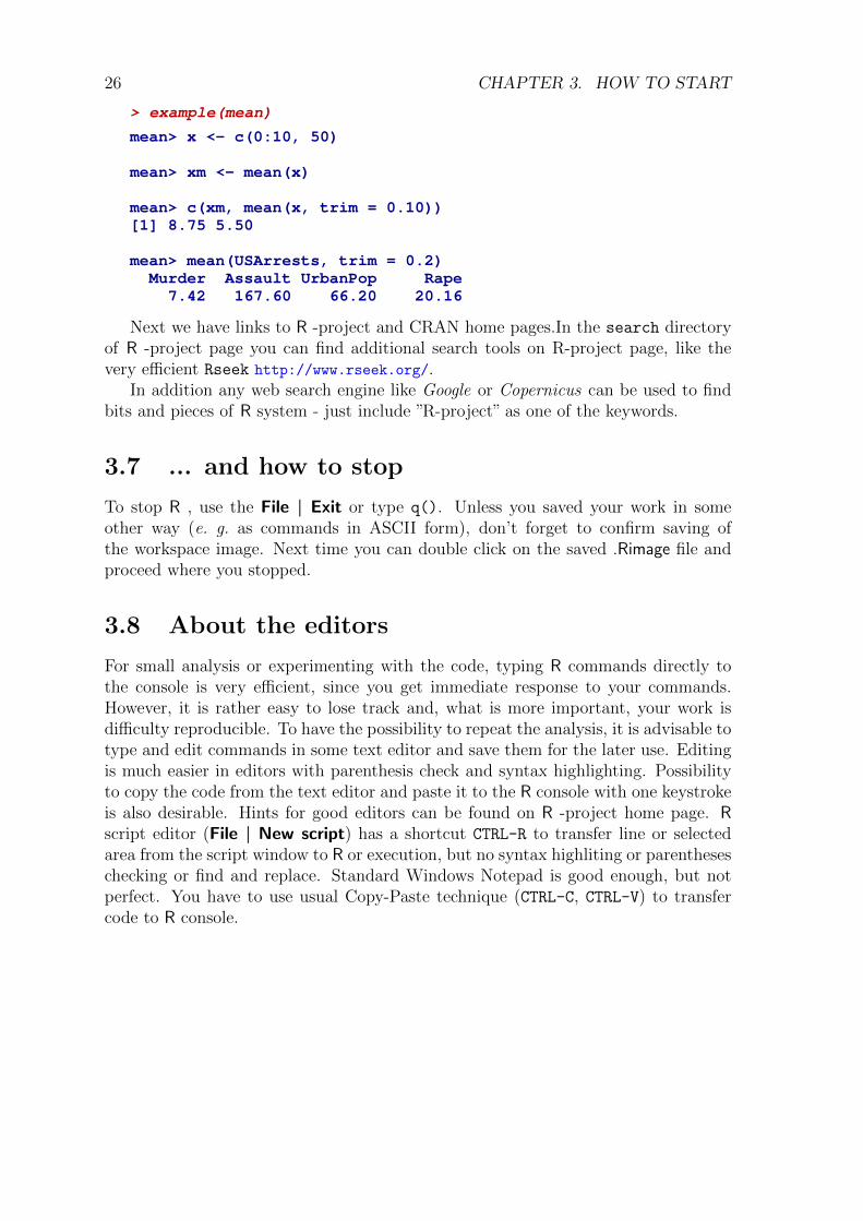
26 CHAPTER 3. HOW TO START
> example(mean)
mean> x <- c(0:10, 50)
mean> xm <- mean(x)
mean> c(xm, mean(x, trim = 0.10))[1] 8.75 5.50
mean> mean(USArrests, trim = 0.2)Murder Assault UrbanPop Rape
7.42 167.60 66.20 20.16
Next we have links to R -project and CRAN home pages.In the search directoryof R -project page you can find additional search tools on R-project page, like thevery efficient Rseek http://www.rseek.org/.
In addition any web search engine like Google or Copernicus can be used to findbits and pieces of R system - just include ”R-project” as one of the keywords.
3.7 ... and how to stop
To stop R , use the File | Exit or type q(). Unless you saved your work in someother way (e. g. as commands in ASCII form), don’t forget to confirm saving ofthe workspace image. Next time you can double click on the saved .Rimage file andproceed where you stopped.
3.8 About the editors
For small analysis or experimenting with the code, typing R commands directly tothe console is very efficient, since you get immediate response to your commands.However, it is rather easy to lose track and, what is more important, your work isdifficulty reproducible. To have the possibility to repeat the analysis, it is advisable totype and edit commands in some text editor and save them for the later use. Editingis much easier in editors with parenthesis check and syntax highlighting. Possibilityto copy the code from the text editor and paste it to the R console with one keystrokeis also desirable. Hints for good editors can be found on R -project home page. Rscript editor (File | New script) has a shortcut CTRL-R to transfer line or selectedarea from the script window to R or execution, but no syntax highliting or parentheseschecking or find and replace. Standard Windows Notepad is good enough, but notperfect. You have to use usual Copy-Paste technique (CTRL-C, CTRL-V) to transfercode to R console.

4 R objects and data structures
R can be used at different levels. First of all, it can be used as a calculator. It is notto difficult to calculate your BMI :)
In data analysis, data are usually collected into tables. In data tables, columnsare usually data series, or variables and rows represent individual units on whichmeasurements were made. In actual calculations, data series and some results areorganized in vectors and matrices.
R supports organization of data in a form of data.frame and one can organizeand manipulate data as vectors and matrices. Vector (1 dimension) and matrix (2dimensions) are extended by additional dimensions into arrays. The richest structurein R is a list, which can hold a number of elements of any of above classes.
4.1 Data structures
4.1.1 Vector
R operates on named data structures. The simplest data structure is a vector whichis a collection of single entities like numbers. Five numbers 5, 10, 4, 9 and 1 can beorganized as a vector and assigned to a named object:
> x <- c(5, 10, 4, 9, 1)> x
[1] 5 10 4 9 1
We used function c() which can take any number of arguments and combinesthem into a single entity. Assignment operator ’<-’ can be replaced with an equalsign ’=’. Assignment can also be made by a function assign, which will produce avector named y:
> assign("y", c(2, 4, 5, -1, 7))> y
[1] 2 4 5 -1 7
If the statement consist of just the name of an object, its content is printed, likey above. If the statement is an expression, its value is printed and lost, unless it isassigned to some name.
27

28 CHAPTER 4. R OBJECTS AND DATA STRUCTURES
> 1/x
[1] 0.2000000 0.1000000 0.2500000 0.1111111 1.0000000
Vectors have one dimension, called length
> length(x)
[1] 5
4.1.2 Vector arithmetic
One of the R strengths is a vector arithmetic. Arithmetic operations are performedcomponent-wise, which means that in a command
> z <- 2 * x + y - 5> z
[1] 7 19 8 12 4
the first component of z is the sum of the first component of x multiplied by 2 andthe first component of y decreased by 5. Then the second ones are used in calculation,and so forth:
zi = 2xi + yi − 5, i = 1, . . . , 5
.The arithmetic operators are the usual ones:
� + addition� - subtraction� * multiplication� / division� ^ power� - unary minus sign for negative values
If an operand (vector) is shorter than the longest one, it is cyclically repeated andcomponents are reused to fulfill the positional demands. Number 5 above was usedfive times.
> x
[1] 5 10 4 9 1
> x * c(-1, 1)
[1] -5 10 -4 9 -1
4.1.3 Generating regular sequences
Regular sequences are often needed and can be made by operator ’:’ or functionseq(). The first version can generate increasing or decreasing sequences of integernumbers - step is always 1 or −1.

4.1. DATA STRUCTURES 29
> 1:5
[1] 1 2 3 4 5
> 4:10
[1] 4 5 6 7 8 9 10
> 9:5
[1] 9 8 7 6 5
> -3:5
[1] -3 -2 -1 0 1 2 3 4 5
> -3:(-5)
[1] -3 -4 -5
> -(3:5)
[1] -3 -4 -5
Function seq can take any step (argument by):
> seq(1, 5)
[1] 1 2 3 4 5
> seq(1, 5, 0.5)
[1] 1.0 1.5 2.0 2.5 3.0 3.5 4.0 4.5 5.0
> seq(from = 1, to = 5, by = 0.5)
[1] 1.0 1.5 2.0 2.5 3.0 3.5 4.0 4.5 5.0
> seq(-3, 6, 2)
[1] -3 -1 1 3 5
> seq(6, -3, -3)
[1] 6 3 0 -3
> seq(length = 5, from = 2, by = 0.5)
[1] 2.0 2.5 3.0 3.5 4.0
Another useful function is rep which repeats arguments certain number of times.
> rep(1, 5)
[1] 1 1 1 1 1
> rep(c(1, 2), 3)
[1] 1 2 1 2 1 2
> rep(c(1, 2), each = 3)
[1] 1 1 1 2 2 2
4.1.4 Missing values
In some cases values of a vector are not known, are missing. Missing values in R havea code NA. In general, in any operation with NA, the value becomes NA. Functionis.na tests which values are missing.
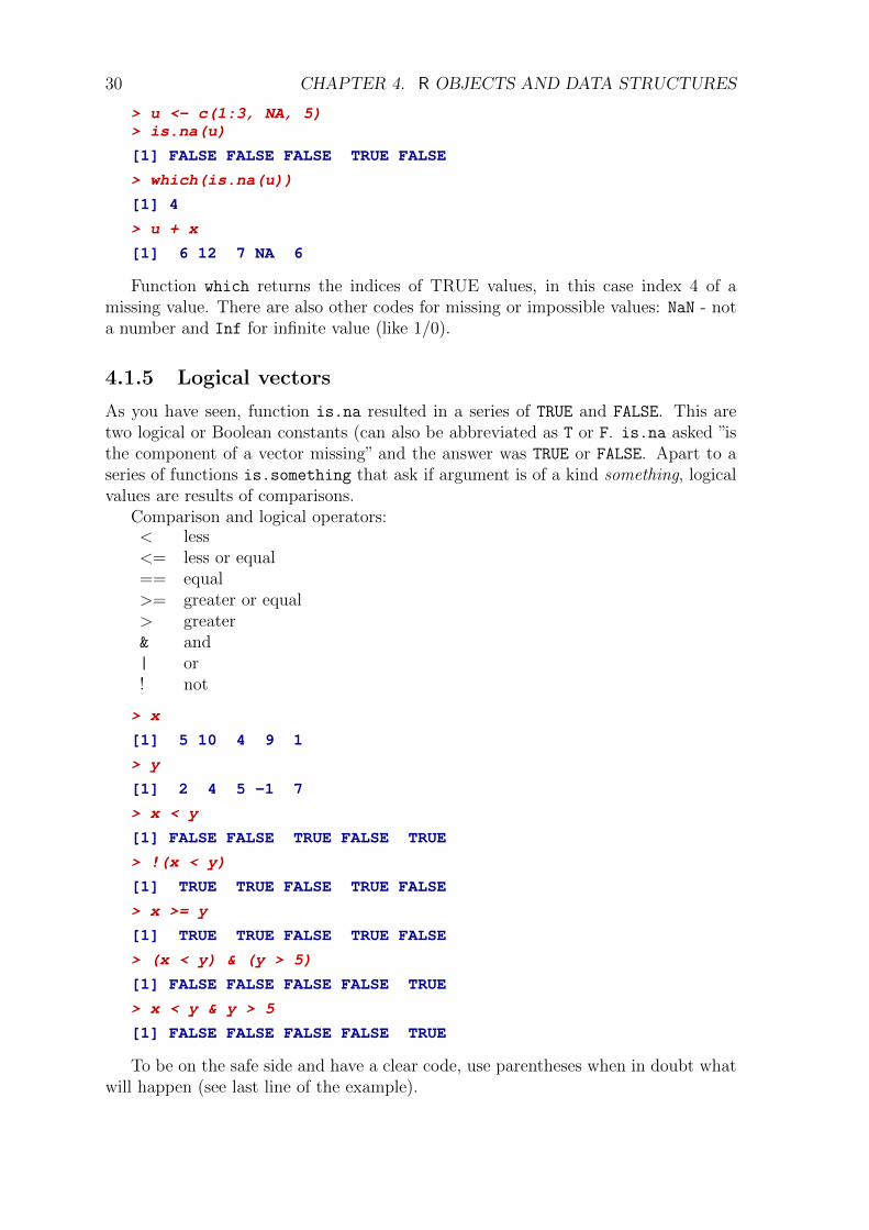
30 CHAPTER 4. R OBJECTS AND DATA STRUCTURES
> u <- c(1:3, NA, 5)> is.na(u)
[1] FALSE FALSE FALSE TRUE FALSE
> which(is.na(u))
[1] 4
> u + x
[1] 6 12 7 NA 6
Function which returns the indices of TRUE values, in this case index 4 of amissing value. There are also other codes for missing or impossible values: NaN - nota number and Inf for infinite value (like 1/0).
4.1.5 Logical vectors
As you have seen, function is.na resulted in a series of TRUE and FALSE. This aretwo logical or Boolean constants (can also be abbreviated as T or F. is.na asked ”isthe component of a vector missing” and the answer was TRUE or FALSE. Apart to aseries of functions is.something that ask if argument is of a kind something, logicalvalues are results of comparisons.
Comparison and logical operators:< less<= less or equal== equal>= greater or equal> greater& and| or! not
> x
[1] 5 10 4 9 1
> y
[1] 2 4 5 -1 7
> x < y
[1] FALSE FALSE TRUE FALSE TRUE
> !(x < y)
[1] TRUE TRUE FALSE TRUE FALSE
> x >= y
[1] TRUE TRUE FALSE TRUE FALSE
> (x < y) & (y > 5)
[1] FALSE FALSE FALSE FALSE TRUE
> x < y & y > 5
[1] FALSE FALSE FALSE FALSE TRUE
To be on the safe side and have a clear code, use parentheses when in doubt whatwill happen (see last line of the example).

4.1. DATA STRUCTURES 314.1.6 Logical vectors as filters
To show use of logical values as filters, we will use small dataset with four variables:
> smallData <- read.table("../dat/filter.txt", header = TRUE)> smallData
g xx yy zz1 M 1 5 12 F 2 8 03 F 3 7 54 M 4 6 85 M 5 3 6
> attach(smallData)
Variable g represent gender of cases. For males, we want to add values of x and y
and z and y for females and store new variable as u.First we just calculate the sum of z and y
> u <- zz + yy
This is wrong for males, so we will correct the values for males. With variableselect we will select which elements to change:
> select <- g == "M"> u[select] <- (xx + yy)[select]> u
[1] 6 8 12 10 8
Finally, add new variable to the dataset
> smallData <- cbind(smallData, u)> smallData
g xx yy zz u1 M 1 5 1 62 F 2 8 0 83 F 3 7 5 124 M 4 6 8 105 M 5 3 6 8
> select <- (g == "M") & (yy > 4)> smallData[select, ]
g xx yy zz u1 M 1 5 1 64 M 4 6 8 10
We do not need the attached data anymore:
> detach()
4.1.7 Character vectors
Character values and character vectors are used frequently in R , for example as plotlabels. When needed they are denoted by a sequence of characters delimited by the
32 CHAPTER 4. R OBJECTS AND DATA STRUCTURESdouble quote character, e. g. ”p-value”, ”Results of comparison”. In some prints andplots, they are used without the quote characters.
Character values can be entered using the double ()̈ or single (’) quotes.
> varname <- c("X", "Y", "Z", "U", "V")> varname
[1] "X" "Y" "Z" "U" "V"
Character values (strings) can be concatenated using paste function.
> paste(varname, x)
[1] "X 5" "Y 10" "Z 4" "U 9" "V 1"
> paste(c("X", "Y"), x, sep = " = ")
[1] "X = 5" "Y = 10" "X = 4" "Y = 9" "X = 1"
> paste("X", x, sep = " = ", collapse = " , ")
[1] "X = 5 , X = 10 , X = 4 , X = 9 , X = 1"
Function paste operates on components, and cyclically reuses shorter vector ele-ments.
4.1.8 Index vectors
Use of index vectors is a way to select and modify a subset of values. Index vectorsare added in square brackets as selectors to vectors. R recognizes several types ofmissing values.
Vector of positive values
Only the elements with indices in a vector of positive values are selected.
> x[2:4]
[1] 10 4 9
Vector of negative values
Negative value is a sign to omit the value with index equal to the opposite value.
> x[-(2:3)]
[1] 5 9 1
Logical vectors
They have to be of the same size as the subsetting vector. The values correspondingto TRUE are selected, those corresponding to FALSE are omitted.

4.1. DATA STRUCTURES 33
> x
[1] 5 10 4 9 1
> u
[1] 6 8 12 10 8
> !is.na(u)
[1] TRUE TRUE TRUE TRUE TRUE
> x[!is.na(u)]
[1] 5 10 4 9 1
This selects elements with missing values:
> (miss <- which(is.na(u)))
integer(0)
> x[miss]
numeric(0)
Vector of character strings
Elements, corresponding the character strings are selected.
> names(x) <- varname> x
X Y Z U V5 10 4 9 1
> x[c("U", "V")]
U V9 1
> names(x) <- NULL
4.1.9 Matrix
Matrix is a collection of vectors (or rows). Matrices can be generated in several ways:
Binding vectors
Vectors can be bind as rows (rbind) or as columns (cbind)
34 CHAPTER 4. R OBJECTS AND DATA STRUCTURES
> cbind(x, y, z)
x y z[1,] 5 2 7[2,] 10 4 19[3,] 4 5 8[4,] 9 -1 12[5,] 1 7 4
> rbind(x, y, z)
[,1] [,2] [,3] [,4] [,5]x 5 10 4 9 1y 2 4 5 -1 7z 7 19 8 12 4
Reshaping a vector into a matrix
> m <- c(x, y, z)> m
[1] 5 10 4 9 1 2 4 5 -1 7 7 19 8 12 4
> X <- matrix(m, 5, 3)> X
[,1] [,2] [,3][1,] 5 2 7[2,] 10 4 19[3,] 4 5 8[4,] 9 -1 12[5,] 1 7 4
> dim(X)
[1] 5 3
A matrix with dimension (5,3) is produced, elements of a vector are columnwisefilled into a matrix (can be changed by argument byrow=TRUE.
Matrices have two dimensions, number of rows and number of columns.
4.1.10 Some operations on matrices
extraction of diagonal diag
> diag(X)
[1] 5 4 8
Transposition (t)
> t(X)
[,1] [,2] [,3] [,4] [,5][1,] 5 10 4 9 1[2,] 2 4 5 -1 7[3,] 7 19 8 12 4
4.1. DATA STRUCTURES 354.1.11 Matrix multiplication %*%
Function scale is used for standardization of data matrix. In our case, just thecolumn means are subtracted from each column. Then the sample covariance matrixis calculated in two ways: by explicit matrix multiplication and by function var.
> (Y <- scale(X, scale = FALSE))
[,1] [,2] [,3][1,] -0.8 -1.4 -3[2,] 4.2 0.6 9[3,] -1.8 1.6 -2[4,] 3.2 -4.4 2[5,] -4.8 3.6 -6attr(,"scaled:center")[1] 5.8 3.4 10.0
> n <- dim(Y)[1]> t(Y) %*% Y/(n - 1)
[,1] [,2] [,3][1,] 13.70 -7.65 19.75[2,] -7.65 9.30 -6.00[3,] 19.75 -6.00 33.50
> var(Y)
[,1] [,2] [,3][1,] 13.70 -7.65 19.75[2,] -7.65 9.30 -6.00[3,] 19.75 -6.00 33.50
4.1.12 Arrays
Arrays are extension of a matrix, they have more than two dimensions.
> array(1:12, c(2, 3, 2))
, , 1
[,1] [,2] [,3][1,] 1 3 5[2,] 2 4 6
, , 2
[,1] [,2] [,3][1,] 7 9 11[2,] 8 10 12
4.1.13 Data frame
Vectors, matrices and arrays can only hold values of the same type: either numericor character or logical. Data frames can have columns of different type. An exampleis bmiData.
Different types of data will be collected by column, but columns have to have thesame length!
36 CHAPTER 4. R OBJECTS AND DATA STRUCTURES
> case <- paste("Case00", 1:5, sep = "-")> xData <- data.frame(case, first = y, second = u, z, miss.u = is.na(u))> xData
case first second z miss.u1 Case00-1 2 6 7 FALSE2 Case00-2 4 8 19 FALSE3 Case00-3 5 12 8 FALSE4 Case00-4 -1 10 12 FALSE5 Case00-5 7 8 4 FALSE
Use cbind and rbind to add additional columns and rows.
List
List is the richest structure in R . It can incorporate components of any kind.
> lst <- list(case, x, p = 0.05, data = xData)> lst
[[1]][1] "Case00-1" "Case00-2" "Case00-3" "Case00-4" "Case00-5"
[[2]][1] 5 10 4 9 1
$p[1] 0.05
$datacase first second z miss.u
1 Case00-1 2 6 7 FALSE2 Case00-2 4 8 19 FALSE3 Case00-3 5 12 8 FALSE4 Case00-4 -1 10 12 FALSE5 Case00-5 7 8 4 FALSE
Components may be named. In any case, one can extract the component bynumber.
> lst[[2]]
[1] 5 10 4 9 1
> lst$p
[1] 0.05
> lst[["p"]]
[1] 0.05
The first line prints the second component. The second and third line extract the p
value.Use use function combine c to add additional components to lists.
> extendedlst <- c(lst, added = "added component")

4.2. GETTING INFORMATION ABOUT DATA STRUCTURES 374.2 Getting information about data structures
We have the following objects: vector x, matrix X, data.frame xData and list lst.
> x
[1] 5 10 4 9 1
> X
[,1] [,2] [,3][1,] 5 2 7[2,] 10 4 19[3,] 4 5 8[4,] 9 -1 12[5,] 1 7 4
> xData
case first second z miss.u1 Case00-1 2 6 7 FALSE2 Case00-2 4 8 19 FALSE3 Case00-3 5 12 8 FALSE4 Case00-4 -1 10 12 FALSE5 Case00-5 7 8 4 FALSE
> lst
[[1]][1] "Case00-1" "Case00-2" "Case00-3" "Case00-4" "Case00-5"
[[2]][1] 5 10 4 9 1
$p[1] 0.05
$datacase first second z miss.u
1 Case00-1 2 6 7 FALSE2 Case00-2 4 8 19 FALSE3 Case00-3 5 12 8 FALSE4 Case00-4 -1 10 12 FALSE5 Case00-5 7 8 4 FALSE
Several functions can give you information about the objects.
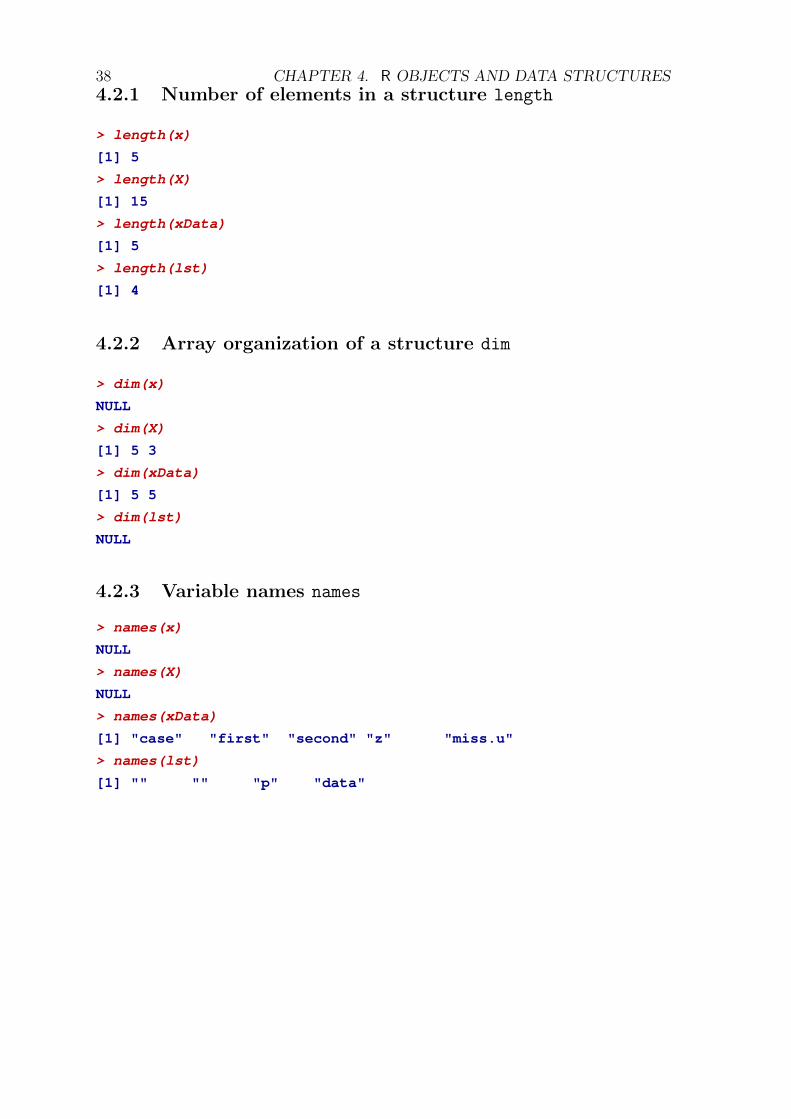
38 CHAPTER 4. R OBJECTS AND DATA STRUCTURES4.2.1 Number of elements in a structure length
> length(x)
[1] 5
> length(X)
[1] 15
> length(xData)
[1] 5
> length(lst)
[1] 4
4.2.2 Array organization of a structure dim
> dim(x)
NULL
> dim(X)
[1] 5 3
> dim(xData)
[1] 5 5
> dim(lst)
NULL
4.2.3 Variable names names
> names(x)
NULL
> names(X)
NULL
> names(xData)
[1] "case" "first" "second" "z" "miss.u"
> names(lst)
[1] "" "" "p" "data"

4.3. SELECTING COLUMNS AND ROWS 394.2.4 Dimension names of an array dimnames
> dimnames(x)
NULL
> dimnames(X)
NULL
> dimnames(xData)
[[1]][1] "1" "2" "3" "4" "5"
[[2]][1] "case" "first" "second" "z" "miss.u"
> dimnames(lst)
NULL
4.2.5 Object structure str
> str(x)
num [1:5] 5 10 4 9 1
> str(X)
num [1:5, 1:3] 5 10 4 9 1 2 4 5 -1 7 ...
> str(xData)
'data.frame': 5 obs. of 5 variables:$ case : Factor w/ 5 levels "Case00-1","Case00-2",..: 1 2 3 4 5$ first : num 2 4 5 -1 7$ second: int 6 8 12 10 8$ z : num 7 19 8 12 4$ miss.u: logi FALSE FALSE FALSE FALSE FALSE
> str(lst)
List of 4$ : chr [1:5] "Case00-1" "Case00-2" "Case00-3" "Case00-4" ...$ : num [1:5] 5 10 4 9 1$ p : num 0.05$ data:'data.frame': 5 obs. of 5 variables:..$ case : Factor w/ 5 levels "Case00-1","Case00-2",..: 1 2 3 4 5..$ first : num [1:5] 2 4 5 -1 7..$ second: int [1:5] 6 8 12 10 8..$ z : num [1:5] 7 19 8 12 4..$ miss.u: logi [1:5] FALSE FALSE FALSE FALSE FALSE
4.3 Selecting columns and rows
Rows and columns can be selected from matrices and data frames.

40 CHAPTER 4. R OBJECTS AND DATA STRUCTURES
> X
[,1] [,2] [,3][1,] 5 2 7[2,] 10 4 19[3,] 4 5 8[4,] 9 -1 12[5,] 1 7 4
> X[2,3] # element in row 2, col 4
[1] 19
> X[2,] # second row
[1] 10 4 19
> X[,c(1,3)] # column 1 and 3
[,1] [,2][1,] 5 7[2,] 10 19[3,] 4 8[4,] 9 12[5,] 1 4
> xData
case first second z miss.u1 Case00-1 2 6 7 FALSE2 Case00-2 4 8 19 FALSE3 Case00-3 5 12 8 FALSE4 Case00-4 -1 10 12 FALSE5 Case00-5 7 8 4 FALSE
> xData[,3] # column 3
[1] 6 8 12 10 8
> xData[,"second"]# column with name "second"
[1] 6 8 12 10 8
> xData[2:4,] # rows 2,3, and 4
case first second z miss.u2 Case00-2 4 8 19 FALSE3 Case00-3 5 12 8 FALSE4 Case00-4 -1 10 12 FALSE
4.4 Replacing values
Values can be replaced by assigning new values to an referenced element. Functionwhich can give also the array indices, useful for replacement of missing data.
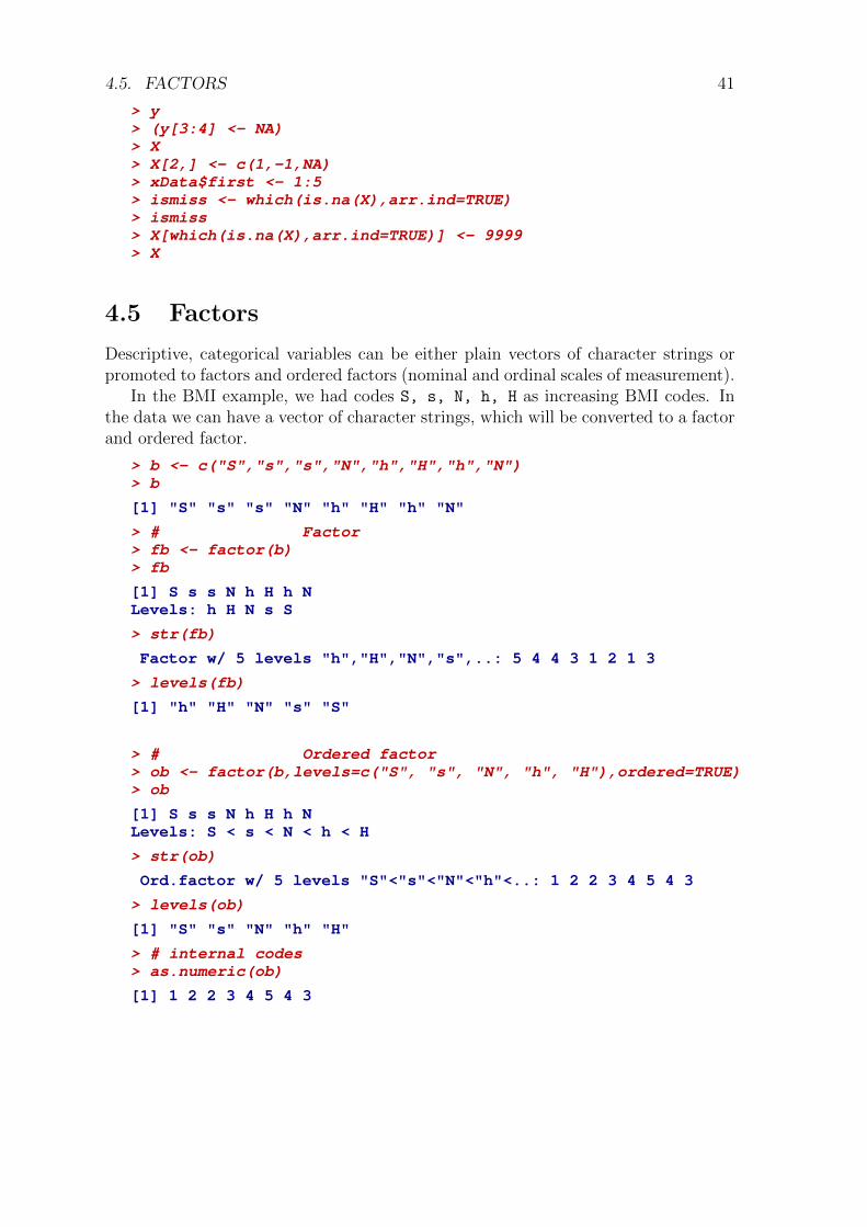
4.5. FACTORS 41
> y> (y[3:4] <- NA)> X> X[2,] <- c(1,-1,NA)> xData$first <- 1:5> ismiss <- which(is.na(X),arr.ind=TRUE)> ismiss> X[which(is.na(X),arr.ind=TRUE)] <- 9999> X
4.5 Factors
Descriptive, categorical variables can be either plain vectors of character strings orpromoted to factors and ordered factors (nominal and ordinal scales of measurement).
In the BMI example, we had codes S, s, N, h, H as increasing BMI codes. Inthe data we can have a vector of character strings, which will be converted to a factorand ordered factor.
> b <- c("S","s","s","N","h","H","h","N")> b
[1] "S" "s" "s" "N" "h" "H" "h" "N"
> # Factor> fb <- factor(b)> fb
[1] S s s N h H h NLevels: h H N s S
> str(fb)
Factor w/ 5 levels "h","H","N","s",..: 5 4 4 3 1 2 1 3
> levels(fb)
[1] "h" "H" "N" "s" "S"
> # Ordered factor> ob <- factor(b,levels=c("S", "s", "N", "h", "H"),ordered=TRUE)> ob
[1] S s s N h H h NLevels: S < s < N < h < H
> str(ob)
Ord.factor w/ 5 levels "S"<"s"<"N"<"h"<..: 1 2 2 3 4 5 4 3
> levels(ob)
[1] "S" "s" "N" "h" "H"
> # internal codes> as.numeric(ob)
[1] 1 2 2 3 4 5 4 3
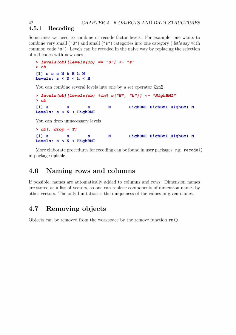
42 CHAPTER 4. R OBJECTS AND DATA STRUCTURES4.5.1 Recoding
Sometimes we need to combine or recode factor levels. For example, one wants tocombine very small ("S") and small ("s") categories into one category ( let’s say withcommon code "s"). Levels can be recoded in the naive way by replacing the selectionof old codes with new ones.
> levels(ob)[levels(ob) == "S"] <- "s"> ob
[1] s s s N h H h NLevels: s < N < h < H
You can combine several levels into one by a set operator %in%.
> levels(ob)[levels(ob) %in% c("H", "h")] <- "HighBMI"> ob
[1] s s s N HighBMI HighBMI HighBMI NLevels: s < N < HighBMI
You can drop unnecessary levels
> ob[, drop = T]
[1] s s s N HighBMI HighBMI HighBMI NLevels: s < N < HighBMI
More elaborate procedures for recoding can be found in user packages, e.g. recode()in package epicalc.
4.6 Naming rows and columns
If possible, names are automatically added to columns and rows. Dimension namesare stored as a list of vectors, so one can replace components of dimension names byother vectors. The only limitation is the uniqueness of the values in given names.
4.7 Removing objects
Objects can be removed from the workspace by the remove function rm().

5 Data import/export
The main function for file reading and writing are functions read.table and write.table
with modifications. Tab delimited text files are the most convenient form of data forinput. R is capable of reading and writing data from many sources and data for-mats. You can use R to exchange files on the local machine, network or eve onthe Internet. It can read data tables in various native formats for many statisti-cal packages. Many data interface functions are described in the package foreign.Package Hmisc has enhanced versions of functions for reading and writing SPSS,STATA, and SAS data. Excel interface is available in package xlsReadWrite. An-other option is to use ODBC interface available in package RODBC. You can also usefunction read.xls() from package gdata, which can be used on all platforms. lfn <-normalizePath(”../dat/birthdeath.xls”) X2<-read.xls(lfn,from=2,rowNames=TRUE)X2 You can find additional information on the R-project web page, accessible alsothrough the Help | Manuals (in PDF) | R Data Import/Export. You can find someexamples in the Appendix.
43
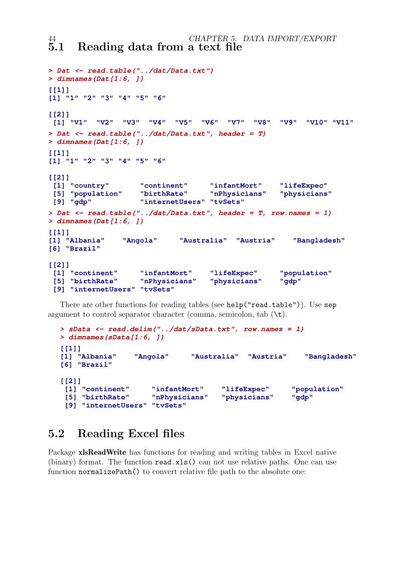
44 CHAPTER 5. DATA IMPORT/EXPORT5.1 Reading data from a text file
> Dat <- read.table("../dat/Data.txt")> dimnames(Dat[1:6, ])
[[1]][1] "1" "2" "3" "4" "5" "6"
[[2]][1] "V1" "V2" "V3" "V4" "V5" "V6" "V7" "V8" "V9" "V10" "V11"
> Dat <- read.table("../dat/Data.txt", header = T)> dimnames(Dat[1:6, ])
[[1]][1] "1" "2" "3" "4" "5" "6"
[[2]][1] "country" "continent" "infantMort" "lifeExpec"[5] "population" "birthRate" "nPhysicians" "physicians"[9] "gdp" "internetUsers" "tvSets"
> Dat <- read.table("../dat/Data.txt", header = T, row.names = 1)> dimnames(Dat[1:6, ])
[[1]][1] "Albania" "Angola" "Australia" "Austria" "Bangladesh"[6] "Brazil"
[[2]][1] "continent" "infantMort" "lifeExpec" "population"[5] "birthRate" "nPhysicians" "physicians" "gdp"[9] "internetUsers" "tvSets"
There are other functions for reading tables (see help("read.table")). Use sep
argument to control separator character (comma, semicolon, tab (\t).
> sData <- read.delim("../dat/sData.txt", row.names = 1)> dimnames(sData[1:6, ])
[[1]][1] "Albania" "Angola" "Australia" "Austria" "Bangladesh"[6] "Brazil"
[[2]][1] "continent" "infantMort" "lifeExpec" "population"[5] "birthRate" "nPhysicians" "physicians" "gdp"[9] "internetUsers" "tvSets"
5.2 Reading Excel files
Package xlsReadWrite has functions for reading and writing tables in Excel native(binary) format. The function read.xls() can not use relative paths. One can usefunction normalizePath() to convert relative file path to the absolute one:

5.2. READING EXCEL FILES 45
> library("xlsReadWrite")> (lfn <- normalizePath("../dat/bmiall.xls"))
[1] "C:\\_Y\\R\\I2R\\dat\\bmiall.xls"
> bmiData <- read.xls(lfn)> head(bmiData)
gender age weight height1 M 17 73.6 1.7302 M 17 71.0 1.7653 M 17 62.4 1.7704 M 17 71.0 1.8705 M 17 72.4 1.7656 M 17 104.0 1.825
To skip first few lines of the Excel table use argument from. By argumentrowNames=TRUE, first column will be used for row names. Argument sheet deter-mines which sheet to read.

46 CHAPTER 5. DATA IMPORT/EXPORT
> lfn <- normalizePath("../dat/birthdeath.xls")> X2 <- read.xls(lfn, from = 2, rowNames = TRUE)> X2
X2007 X2006 X2005 X1990 X1985 X1980 X1975 X2007 X2006 X2005Australia 12.0 12.1 12.3 15.4 15.7 15.3 16.9 7.6 7.5 7.4Austria 8.7 8.7 8.8 11.6 11.6 12.0 12.5 9.8 9.8 9.7Belgium 10.3 10.4 10.5 12.6 11.5 12.7 12.2 10.3 10.3 10.2Czech Republic1 9.0 9.0 9.1 13.4 14.5 16.4 19.6 10.6 10.6 10.5France 11.9 12.0 12.2 13.5 13.9 14.8 14.1 9.2 9.1 9.1Germany2 8.2 8.3 8.3 11.4 9.6 10.0 9.7 10.7 10.6 10.6Greece 9.6 9.7 9.7 10.2 11.7 15.4 15.7 10.3 10.2 10.2Ireland 14.4 14.5 14.5 15.1 17.6 21.9 21.5 7.8 7.8 7.8Israel 17.7 18.0 18.2 22.2 23.5 24.1 28.2 6.2 6.2 6.2Italy 8.5 8.7 8.9 9.8 10.1 11.2 14.8 10.5 10.4 10.3Japan 9.2 9.4 9.5 9.9 11.9 13.7 17.2 9.4 9.2 9.0Mauritius 15.3 15.4 15.6 21.0 18.8 27.0 25.1 6.9 6.9 6.8Netherlands 10.7 10.9 11.1 13.3 12.3 12.8 13.0 8.7 8.7 8.7New Zealand 13.6 13.8 13.9 18.0 15.6 NaN 18.4 7.5 7.5 7.5Norway 11.3 11.5 11.7 14.3 12.3 12.5 14.1 9.4 9.4 9.5Panama 21.5 21.7 22.0 23.9 26.6 26.8 32.3 5.4 5.4 5.3Poland 9.9 9.9 9.7 14.3 18.2 19.5 18.9 9.9 9.9 9.8Portugal 10.6 10.7 10.8 11.8 12.8 16.4 19.1 10.6 10.5 10.4Romania 10.7 10.7 10.7 13.6 15.8 NaN NaN 11.8 11.8 11.7Switzerland 9.7 9.7 9.8 12.5 11.6 11.3 12.3 8.5 8.5 8.5Tunisia 15.5 15.5 15.5 25.8 31.3 35.2 36.6 5.2 5.1 5.1United Kingdom 10.7 10.7 10.8 13.9 13.3 13.5 12.5 10.1 10.1 10.2United States 14.2 14.1 14.1 16.7 15.7 16.2 14.0 8.3 8.3 8.2
X1990 X1985 X1980 X1975Australia 7.0 7.5 7.4 7.9Austria 10.6 11.9 12.2 12.8Belgium 10.6 11.2 11.6 12.2Czech Republic1 11.7 11.8 12.1 11.5France 9.3 10.1 10.2 10.6Germany2 11.2 11.5 11.6 12.1Greece 9.3 9.4 9.1 8.9Ireland 9.1 9.4 9.7 10.6Israel 6.2 6.6 6.7 7.1Italy 9.4 9.5 9.7 9.9Japan 6.7 6.2 6.2 6.4Mauritius 6.5 6.8 7.2 8.1Netherlands 8.6 8.5 8.1 8.3New Zealand 7.9 8.4 NaN 8.1Norway 10.7 10.7 10.1 9.9Panama NaN NaN NaN NaNPoland 10.2 10.3 9.8 8.7Portugal 10.4 9.6 9.9 10.4Romania 10.6 10.9 NaN NaNSwitzerland 9.5 9.2 9.2 8.7Tunisia NaN NaN NaN NaNUnited Kingdom 11.2 11.8 11.8 11.9United States 8.6 8.7 8.9 8.9
If you look at the file birthdeath.xls, you will see why we have to start readingin the second row and that the first seven columns describe the birth rates while thenext seven record the death rates in seven years. When the data were read into R ,

5.2. READING EXCEL FILES 47column names (years) were prefixed by ”X” to make legal names. The following codemakes more reasonable names.
> (years <- substring(names(X2), 2, 5))
[1] "2007" "2006" "2005" "1990" "1985" "1980" "1975" "2007" "2006" "2005"[11] "1990" "1985" "1980" "1975"
> names(X2) <- paste(rep(c("birth", "death"), each = 7), years,+ sep = ".")> t(X2[c("Austria", "Italy"), ])
Austria Italybirth.2007 8.7 8.5birth.2006 8.7 8.7birth.2005 8.8 8.9birth.1990 11.6 9.8birth.1985 11.6 10.1birth.1980 12.0 11.2birth.1975 12.5 14.8death.2007 9.8 10.5death.2006 9.8 10.4death.2005 9.7 10.3death.1990 10.6 9.4death.1985 11.9 9.5death.1980 12.2 9.7death.1975 12.8 9.9
Table birthdeath.xls is in a shape more common for results than data. It issummarizing two variables: birth rate and death rate across countries and time. Onecould reshape it into a data frame with four variables: country,year, birthRate,and deathRate
> lfn <- normalizePath("../dat/birthdeath.xls")> X3 <- read.xls(lfn, from = 2)> names(X3)
[1] "Country" "X2007" "X2006" "X2005" "X1990" "X1985" "X1980"[8] "X1975" "X2007" "X2006" "X2005" "X1990" "X1985" "X1980"[15] "X1975"
> years <- as.numeric(sub("^X(.*)", "\\1", names(X3)[-1]))> (years <- unique(years))
[1] 2007 2006 2005 1990 1985 1980 1975
> attach(X3)> X3 <- data.frame(country = as.character(rep(X3[, 1], 7)), year = rep(years,+ each = dim(X3)[1]), birthRate = as.vector(unlist(X3[, 2:8])),+ deathRate = as.vector(unlist(X3[, 9:15])))> detach()> head(X3)
country year birthRate deathRate1 Australia 2007 12.0 7.62 Austria 2007 8.7 9.83 Belgium 2007 10.3 10.34 Czech Republic1 2007 9.0 10.65 France 2007 11.9 9.26 Germany2 2007 8.2 10.7
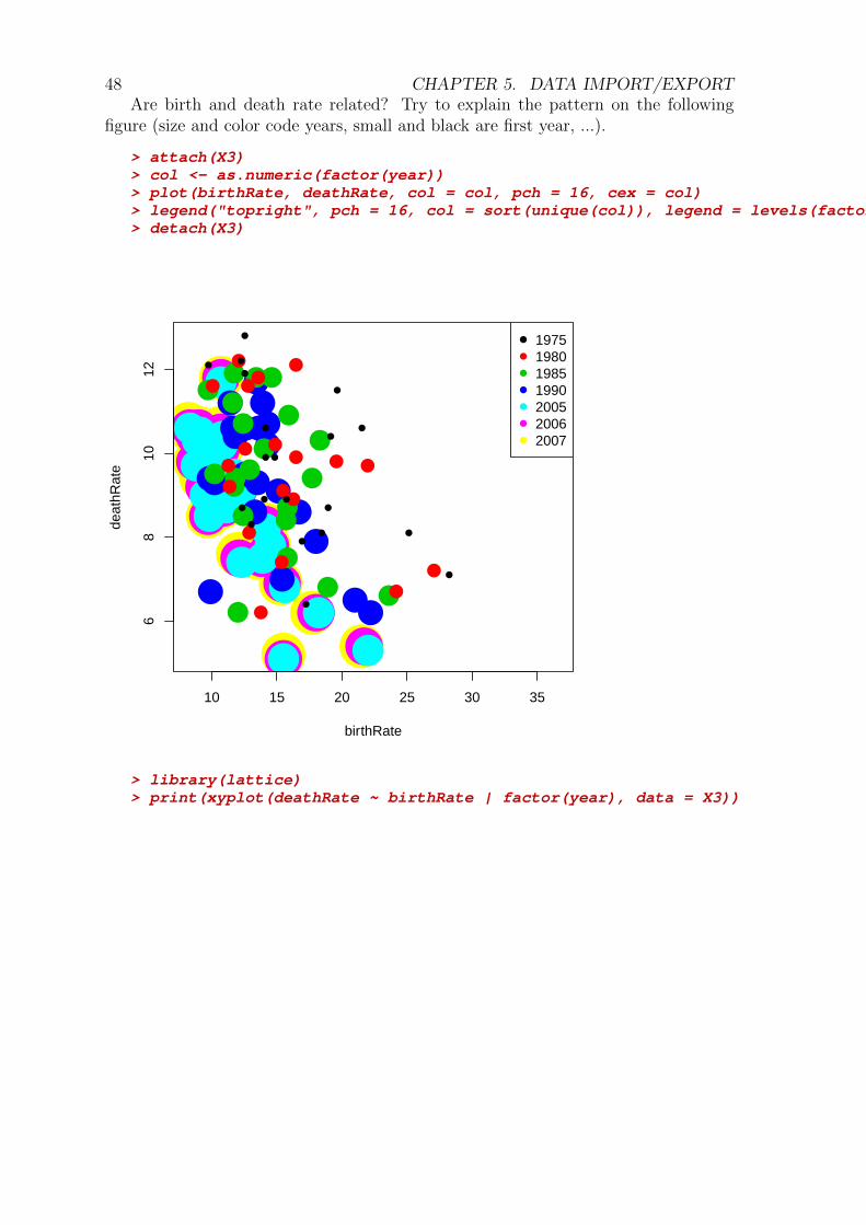
48 CHAPTER 5. DATA IMPORT/EXPORTAre birth and death rate related? Try to explain the pattern on the following
figure (size and color code years, small and black are first year, ...).
> attach(X3)> col <- as.numeric(factor(year))> plot(birthRate, deathRate, col = col, pch = 16, cex = col)> legend("topright", pch = 16, col = sort(unique(col)), legend = levels(factor(year)))> detach(X3)
●
●●
●
●
●
● ●
●
●
●●
● ●
●●
●
●
●
●
●
●
●
●●
●
●
●
●
●
●
●
●
●
●●●
●
●
●
●
●
●
●
●
●
●
●
●
●
●
●●
●
●
●
●
●
●
●
10 15 20 25 30 35
68
1012
birthRate
deat
hRat
e
●
●
●
●
●
●
●
1975198019851990200520062007
> library(lattice)> print(xyplot(deathRate ~ birthRate | factor(year), data = X3))
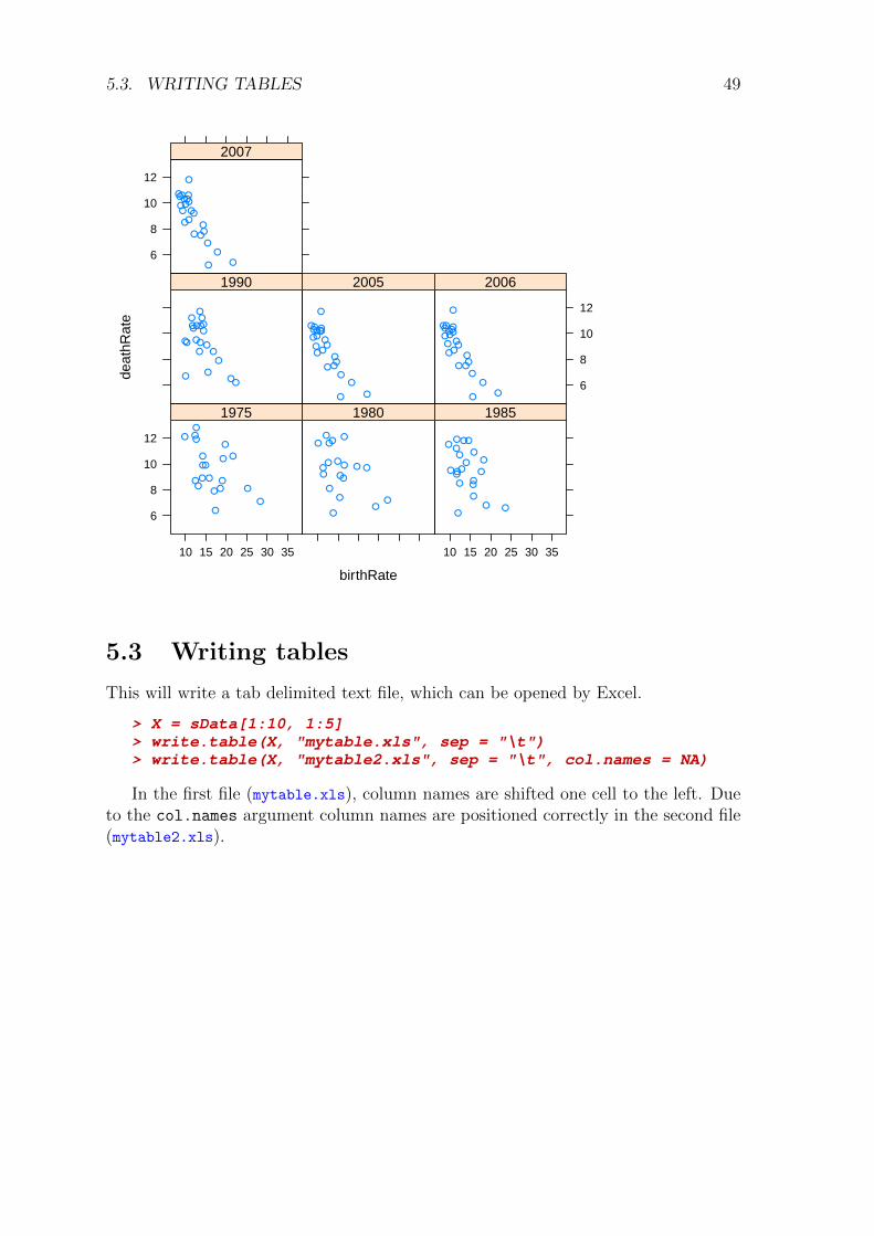
5.3. WRITING TABLES 49
birthRate
deat
hRat
e
6
8
10
12
10 15 20 25 30 35
●
●●
●
●
●
●
●
●
●
●
●● ●
●
●
●
●
●
●
1975
●
●●
●
●
●
●●
●
●
●
●
●
●●●
●
●
●
1980
10 15 20 25 30 35
●
●●
●
●
●
● ●
●
●
●●
● ●
●●
●
●
●
●
●
1985
●
●●
●
●
●
● ●
●
●
● ●
●●
●●● ●
●
●
●
1990
●
●●
●
●
●●
●
●
●
●
●
●
●
●
●
●●
●
●
●
●
●
2005
6
8
10
12
●
●●
●
●
●●
●
●
●
●
●
●
●
●
●
●●
●
●
●
●
●
2006
6
8
10
12
●
●●
●
●
●●
●
●
●
●
●
●
●
●
●
●●
●
●
●
●
●
2007
5.3 Writing tables
This will write a tab delimited text file, which can be opened by Excel.
> X = sData[1:10, 1:5]> write.table(X, "mytable.xls", sep = "\t")> write.table(X, "mytable2.xls", sep = "\t", col.names = NA)
In the first file (mytable.xls), column names are shifted one cell to the left. Dueto the col.names argument column names are positioned correctly in the second file(mytable2.xls).

50 CHAPTER 5. DATA IMPORT/EXPORT5.4 Reading and writing data in statistical package
formats
Functions for reading data in native formats of statistical packages (e.g. SPSS) arein foreign.
5.4.1 Reading SPSS (.SAV) file
Function read.spss returns a list with variable and value labels or a data frame:
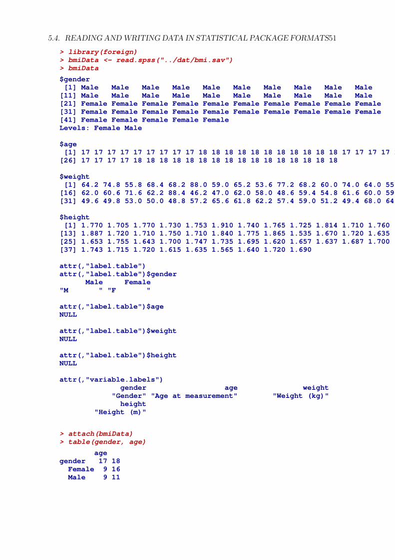
5.4. READING ANDWRITING DATA IN STATISTICAL PACKAGE FORMATS51
> library(foreign)> bmiData <- read.spss("../dat/bmi.sav")> bmiData
$gender[1] Male Male Male Male Male Male Male Male Male Male[11] Male Male Male Male Male Male Male Male Male Male[21] Female Female Female Female Female Female Female Female Female Female[31] Female Female Female Female Female Female Female Female Female Female[41] Female Female Female Female FemaleLevels: Female Male
$age[1] 17 17 17 17 17 17 17 17 17 18 18 18 18 18 18 18 18 18 18 18 17 17 17 17 17[26] 17 17 17 17 18 18 18 18 18 18 18 18 18 18 18 18 18 18 18 18
$weight[1] 64.2 74.8 55.8 68.4 68.2 88.0 59.0 65.2 53.6 77.2 68.2 60.0 74.0 64.0 55.6[16] 62.0 60.6 71.6 62.2 88.4 46.2 47.0 62.0 58.0 48.6 59.4 54.8 61.6 60.0 59.2[31] 49.6 49.8 53.0 50.0 48.8 57.2 65.6 61.8 62.2 57.4 59.0 51.2 49.4 68.0 64.6
$height[1] 1.770 1.705 1.770 1.730 1.753 1.910 1.740 1.765 1.725 1.814 1.710 1.760[13] 1.887 1.720 1.710 1.750 1.710 1.840 1.775 1.865 1.535 1.670 1.720 1.635[25] 1.653 1.755 1.643 1.700 1.747 1.735 1.695 1.620 1.657 1.637 1.687 1.700[37] 1.743 1.715 1.720 1.615 1.635 1.565 1.640 1.720 1.690
attr(,"label.table")attr(,"label.table")$gender
Male Female"M " "F "
attr(,"label.table")$ageNULL
attr(,"label.table")$weightNULL
attr(,"label.table")$heightNULL
attr(,"variable.labels")gender age weight
"Gender" "Age at measurement" "Weight (kg)"height
"Height (m)"
> attach(bmiData)> table(gender, age)
agegender 17 18
Female 9 16Male 9 11

52 CHAPTER 5. DATA IMPORT/EXPORT
> library(foreign)> bmiData <- read.spss("../dat/bmi.sav", to.data.frame = TRUE)> head(bmiData)
gender age weight height1 Male 17 64.2 1.7702 Male 17 74.8 1.7053 Male 17 55.8 1.7704 Male 17 68.4 1.7305 Male 17 68.2 1.7536 Male 17 88.0 1.910
5.4.2 Reading Stata binary file
Function read.dta reads Stata binary files (version 5-10).
5.4.3 Writing in package formats
Function write.foreign exports simple data frames to other statistical packages bywriting the data as free-format text and writing a separate file of instructions for theother package to read the data.
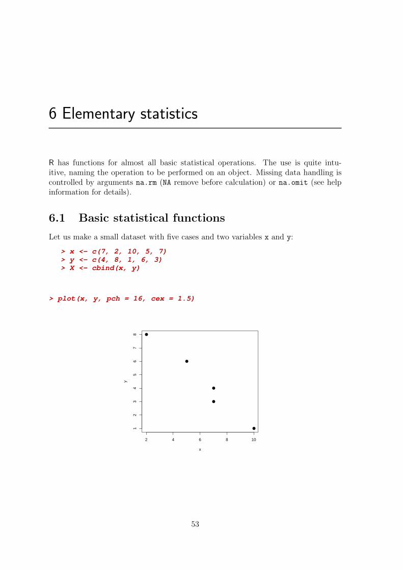
6 Elementary statistics
R has functions for almost all basic statistical operations. The use is quite intu-itive, naming the operation to be performed on an object. Missing data handling iscontrolled by arguments na.rm (NA remove before calculation) or na.omit (see helpinformation for details).
6.1 Basic statistical functions
Let us make a small dataset with five cases and two variables x and y:
> x <- c(7, 2, 10, 5, 7)> y <- c(4, 8, 1, 6, 3)> X <- cbind(x, y)
> plot(x, y, pch = 16, cex = 1.5)
●
●
●
●
●
2 4 6 8 10
12
34
56
78
x
y
53

54 CHAPTER 6. ELEMENTARY STATISTICS6.1.1 Range and sum
> min(x)
[1] 2
> max(x)
[1] 10
> range(x)
[1] 2 10
> sum(x)
[1] 31
> cumsum(x)
[1] 7 9 19 24 31
> cumprod(x)
[1] 7 14 140 700 4900
> diff(x)
[1] -5 8 -5 2
6.1.2 Descriptives
> mean(x)
[1] 6.2
> median(x)
[1] 7
> sd(x)
[1] 2.949576
> sd(X)
x y2.949576 2.701851
> var(x)
[1] 8.7
> var(X)
x yx 8.70 -7.85y -7.85 7.30
> cor(X)
x yx 1.000000 -0.985028y -0.985028 1.000000
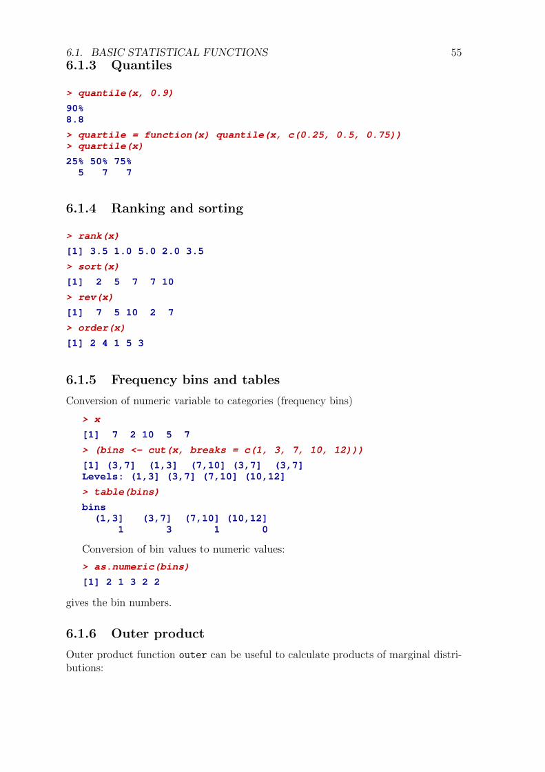
6.1. BASIC STATISTICAL FUNCTIONS 556.1.3 Quantiles
> quantile(x, 0.9)
90%8.8
> quartile = function(x) quantile(x, c(0.25, 0.5, 0.75))> quartile(x)
25% 50% 75%5 7 7
6.1.4 Ranking and sorting
> rank(x)
[1] 3.5 1.0 5.0 2.0 3.5
> sort(x)
[1] 2 5 7 7 10
> rev(x)
[1] 7 5 10 2 7
> order(x)
[1] 2 4 1 5 3
6.1.5 Frequency bins and tables
Conversion of numeric variable to categories (frequency bins)
> x
[1] 7 2 10 5 7
> (bins <- cut(x, breaks = c(1, 3, 7, 10, 12)))
[1] (3,7] (1,3] (7,10] (3,7] (3,7]Levels: (1,3] (3,7] (7,10] (10,12]
> table(bins)
bins(1,3] (3,7] (7,10] (10,12]
1 3 1 0
Conversion of bin values to numeric values:
> as.numeric(bins)
[1] 2 1 3 2 2
gives the bin numbers.
6.1.6 Outer product
Outer product function outer can be useful to calculate products of marginal distri-butions:

56 CHAPTER 6. ELEMENTARY STATISTICS
> a = c(2, 3)> b = c(4, 5)> outer(a, b)
[,1] [,2][1,] 8 10[2,] 12 15
> outer(a, b, paste, sep = "x")
[,1] [,2][1,] "2x4" "2x5"[2,] "3x4" "3x5"
6.1.7 Marginal sums and means
> X
x y[1,] 7 4[2,] 2 8[3,] 10 1[4,] 5 6[5,] 7 3
> colMeans(X)
x y6.2 4.4
> colSums(X)
x y31 22
> rowSums(X)
[1] 11 10 11 11 10
> rowMeans(X)
[1] 5.5 5.0 5.5 5.5 5.0
6.2 apply(): Application of functions to matrix
rows and columns
Function apply can be used to get similar results for arbitrary function that workson vectors: Column (note second argument) and row means
> apply(X, MARGIN = 2, FUN = mean)
x y6.2 4.4
> apply(X, 1, mean)
[1] 5.5 5.0 5.5 5.5 5.0
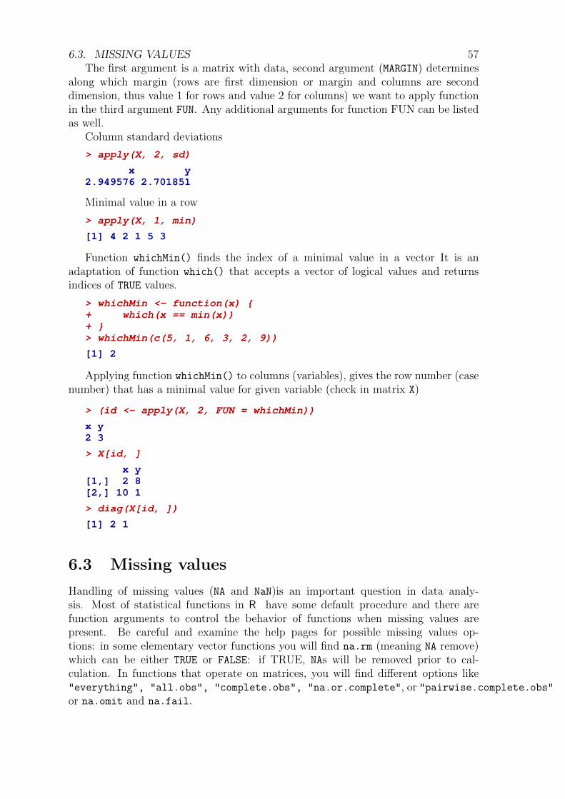
6.3. MISSING VALUES 57The first argument is a matrix with data, second argument (MARGIN) determines
along which margin (rows are first dimension or margin and columns are seconddimension, thus value 1 for rows and value 2 for columns) we want to apply functionin the third argument FUN. Any additional arguments for function FUN can be listedas well.
Column standard deviations
> apply(X, 2, sd)
x y2.949576 2.701851
Minimal value in a row
> apply(X, 1, min)
[1] 4 2 1 5 3
Function whichMin() finds the index of a minimal value in a vector It is anadaptation of function which() that accepts a vector of logical values and returnsindices of TRUE values.
> whichMin <- function(x) {+ which(x == min(x))+ }> whichMin(c(5, 1, 6, 3, 2, 9))
[1] 2
Applying function whichMin() to columns (variables), gives the row number (casenumber) that has a minimal value for given variable (check in matrix X)
> (id <- apply(X, 2, FUN = whichMin))
x y2 3
> X[id, ]
x y[1,] 2 8[2,] 10 1
> diag(X[id, ])
[1] 2 1
6.3 Missing values
Handling of missing values (NA and NaN)is an important question in data analy-sis. Most of statistical functions in R have some default procedure and there arefunction arguments to control the behavior of functions when missing values arepresent. Be careful and examine the help pages for possible missing values op-tions: in some elementary vector functions you will find na.rm (meaning NA remove)which can be either TRUE or FALSE: if TRUE, NAs will be removed prior to cal-culation. In functions that operate on matrices, you will find different options like"everything", "all.obs", "complete.obs", "na.or.complete", or "pairwise.complete.obs"or na.omit and na.fail.

58 CHAPTER 6. ELEMENTARY STATISTICSFunction sum (and many others) have defaulted argument na.rm=FALSE
> args(sum)
function (..., na.rm = FALSE)NULL
and will return result NA if some values are missing.
> z <- c(8, 9, NA, 7, 6)> sum(z)
[1] NA
When we set argument na.rm=TRUE, NAs will be removed prior to calculation:
> sum(z, na.rm = TRUE)
[1] 30
One can remove NAs by use of function is.na: Function is.na returns TRUE ifvalue is missing (NA).
> z
[1] 8 9 NA 7 6
> is.na(z)
[1] FALSE FALSE TRUE FALSE FALSE
> which(is.na(z))
[1] 3
> u <- z[-which(is.na(z))]> u
[1] 8 9 7 6
> sum(u)
[1] 30
Missing values can be replaced by some other value:
> (u <- z)
[1] 8 9 NA 7 6
> u[which(is.na(z))] <- 999> u
[1] 8 9 999 7 6
Mean value imputation:
> (u <- z)
[1] 8 9 NA 7 6
> u[which(is.na(z))] <- mean(u, na.rm = TRUE)> u
[1] 8.0 9.0 7.5 7.0 6.0
Multiple NA replacement
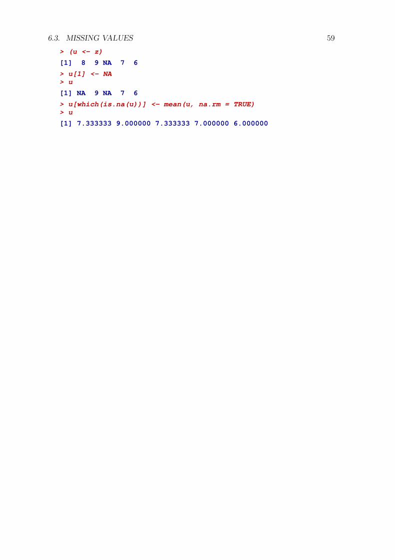
6.3. MISSING VALUES 59
> (u <- z)
[1] 8 9 NA 7 6
> u[1] <- NA> u
[1] NA 9 NA 7 6
> u[which(is.na(u))] <- mean(u, na.rm = TRUE)> u
[1] 7.333333 9.000000 7.333333 7.000000 6.000000

60 CHAPTER 6. ELEMENTARY STATISTICS

7 Writing functions
It pays to pack sequences of commands that are executed together and are used veryoften. You can always copy and paste them from some text editor, but it is a bitclumsy and rigid approach, requiring for example that data are always named in thesame way. A much better style is to pack such commands as a function.
7.1 R functions
All standard R commands are functions. Functions are objects, that can get inputparameters via arguments and perform some operation with a visible or (sometimes)invisible effect. Functions can, for example, receive some data as input; then performsome operation like calculate something, plot some graph, save data to disc; andpossibly return an object with results. The structure of a function is
function( arguments ){
statement 1
statement 2 ...
return( object )
}
A function is a group of expressions (grouped expressions are enclosed in curlybraces {...}) introduced by an argument list. This structure can be assigned to anobject with some name, which is used to invoke this function.
As an example, we will prepare a function that will write data to disk in a styleof the last example in the section Writing tables. We would like to avoid thinkingabout the sep and col.names in future writings of data to disc. We will name thefunction store.table.
> store.table <- function(x, file) {+ write.table(x, file = file, sep = "\t", col.names = NA)+ }
The function has two arguments, the first is an object name (no double quotesneeded!) and the second is the file name (string, quotes needed at function call!)Argument names (x and file are the placeholders and are sort of nickname for actualnames that will be used at the function call. Inside the function, the first argument
61
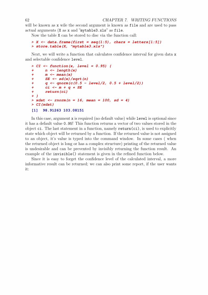
62 CHAPTER 7. WRITING FUNCTIONSwill be known as x wile the second argument is known as file and are used to passactual arguments (X as x and ”mytable3.xls” as file.
Now the table X can be stored to disc via the function call:
> X <- data.frame(first = seq(1:5), chars = letters[1:5])> store.table(X, "mytable3.xls")
Next, we will write a function that calculates confidence interval for given data x
and selectable confidence level.
> CI <- function(x, level = 0.95) {+ n <- length(x)+ m <- mean(x)+ SE <- sd(x)/sqrt(n)+ q <- qnorm(c(0.5 - level/2, 0.5 + level/2))+ ci <- m + q * SE+ return(ci)+ }> xdat <- rnorm(n = 16, mean = 100, sd = 4)> CI(xdat)
[1] 98.91263 103.08151
In this case, argument x is required (no default value) while level is optional sinceit has a default value 0.95! This function returns a vector of two values stored in theobject ci. The last statement in a function, namely return(ci), is used to explicitlystate which object will be returned by a function. If the returned value is not assignedto an object, it’s value is typed into the command window. In some cases ( whenthe returned object is long or has a complex structure) printing of the returned valueis undesirable and can be prevented by invisibly returning the function result. Anexample of the invisible() statement is given in the refined function below.
Since it is easy to forget the confidence level of the calculated interval, a moreinformative result can be returned; we can also print some report, if the user wantsit:
7.2. CONTROL STRUCTURES 63
> CI <- function(x, level = 0.95, verbose = FALSE) {+ n <- length(x)+ m <- mean(x)+ SE <- sd(x)/sqrt(n)+ q <- qnorm(0.5 + c(-level/2, level/2))+ ci <- m + q * SE+ if (verbose) {+ cPerc <- paste(level * 100, "%", sep = "")+ cat(cPerc, "confidence interval: (", ci[1], ",", ci[2],+ ")\n")+ }+ invisible(list(limits = ci, confidence = level))+ }> xdat <- rnorm(n = 16, mean = 100, sd = 4)> CI(xdat)> CI(xdat, verbose = TRUE)
95% confidence interval: ( 97.10493 , 100.5006 )
> interval <- CI(xdat)> interval
$limits[1] 97.10493 100.50056
$confidence[1] 0.95
Using the optional parameter verbose and if statement, we can control whetherthe function itself will report the interval limits or just be silent. We used functioncat to print nicely formatted result. print can print just one object in plain format.In the second call of CI(xdat,verbose=TRUE), the first argument was referenced byposition, and the verbose part was argument was called by name: otherwise it wouldbe treated as level on second position.
7.2 Control structures
R recognizes several control structures, that are usual in other programming lan-guages. Control structures enable looping (repeating the same set of instructions,e.g. for structure) and branching (e.g. if structure).
7.2.1 Looping: for structure
A series of confidence intervals for a set of confidence levels can be produced by usingthe for loop:
for(var in seq) expr
Expression expr will be evaluated for each value in a sequence. In each evaluation,var will take corresponding value from sequence seq.
64 CHAPTER 7. WRITING FUNCTIONS
> for (level in c(0.9, 0.95, 0.99)) CI(xdat, level, TRUE)
90% confidence interval: ( 97.3779 , 100.2276 )95% confidence interval: ( 97.10493 , 100.5006 )99% confidence interval: ( 96.57143 , 101.0341 )
There are other control structures (see help: ?Control).
7.2.2 Branching: if structure
Beside for you will mostly need also if, which can control the operation given thelogical condition:
if(cond) expr
if(cond) expr else alt.expr
In the first case, expression expr will be evaluated only if cond is TRUE. In thesecond form, expression expr will be evaluated if cond is TRUE. otherwise alt.expr
will be evaluated:
> p <- 0.02> alpha <- 0.05> if (p < alpha) cat("p less than alpha\n") else cat("p greater than alpha\n")
p less than alpha

8 Probability distributions
R has a rich family of functions for probability distributions.
Distribution R name additional argumentsbeta beta shape1, shape2, ncpbinomial binom size, probCauchy cauchy location, scalechi-squared chisq df, ncpexponential exp rateF f df1, df2, ncpgamma gamma shape, scalegeometric geom probhypergeometric hyper m, n, klog-normal lnorm meanlog, sdloglogistic logis location, scalenegative binomial nbinom size, probnormal norm mean, sdPoisson pois lambdaStudent’s t t df, ncpuniform unif min, maxWeibull weibull shape, scaleWilcoxon wilcox m, n
”R name” should be preceded by one of the prefix letter to get the actual function:
prefix call meaningd dnorm(x,...) density at xp pnorm(q, ...) cumulative probability up to q P (x ≤ q)c qnorm(p, ...) quantile xpr rnorm(n, ...) n random numbers
For normal distribution we get:
65

66 CHAPTER 8. PROBABILITY DISTRIBUTIONS
> dnorm(0) # density at 0; standardized normal distribution
[1] 0.3989423
> pnorm(1.96) # cumulative distribution P(Z<1.96)
[1] 0.9750021
> qnorm(0.975) # quantile for p=0.975
[1] 1.959964
> rnorm(5) # 5 random numbers
[1] 0.89980762 0.06208036 -1.06860811 0.76641523 0.57688349
By use of these functions, one can plot distributions, get probabilities for test, andgenerate random numbers for simulations.
> curve(dnorm(x),xlim=c(-4,4)) # plot a curve for a function> abline(h=0) # horizontal line at 0
−4 −2 0 2 4
0.0
0.1
0.2
0.3
0.4
x
dnor
m(x
)
8.1 Sampling distribution
Sampling distribution is a distribution of estimates. To demonstrate its features,we can perform an repeated sampling experiment. First we will generate N = 100samples with a sample size n = 9 normally distributed random numbers. We willorganize them into a N×n matrix and compute mean values (by rows) for all samples.

8.1. SAMPLING DISTRIBUTION 67Computation with apply is much more efficient than a use of for statement. Thenwe will plot the histogram of original data and the histogram of estimates.
> N=100> n=9> X=rnorm(N*n) # generate random numbers> X=matrix(X,N,n) # reshape them into a N x n matrix> M=apply(X,1,mean) # calculate the vector of means> head(M) # display first few
[1] 0.57322707 -0.33556026 -0.17591202 -0.37841970 0.02554139 0.10454295
> range(M) # display the range of estimates
[1] -0.5862528 0.6972450
> #> par(mfrow=c(2,1)) # organize space for plots in 2 rows, 1 column> (xlimits=range(X)) # get the range of sampled values
[1] -2.878217 2.818998
> hist(X,prob=TRUE,xlim=xlimits,col="lightgreen",main="Distribution of X")> hist(M,prob=TRUE,xlim=xlimits,col="lightblue",main="Distribution of estimates")
Distribution of X
X
Den
sity
−3 −2 −1 0 1 2 3
0.0
0.2
Distribution of estimates
M
Den
sity
−3 −2 −1 0 1 2 3
0.0
1.0

68 CHAPTER 8. PROBABILITY DISTRIBUTIONSConverting this to a function, gives us a lot o possibilities for different experiments:
> sDist <- function(N=100,n=9,DIST=rnorm,FUN=mean,...){+ X=DIST(N*n,...) # generate random numbers+ X=matrix(X,N,n) # reshape them into a N x n matrix+ M=apply(X,1,FUN) # calculate the vector of means+ head(M) # display first few+ range(M) # display the range of estimates+ #+ par(mfrow=c(2,1)) # organize space for plots in 2 rows, 1 column+ (xlimits=range(X)) # get the range of sampled values+ hist(X,prob=TRUE,xlim=xlimits,col="lightgreen",+ main="Distribution of X")+ hist(M,prob=TRUE,xlim=xlimits,col="lightblue",+ main="Distribution of estimates")+ }> sDist(100,9,DIST=runif)
Distribution of X
X
Den
sity
0.0 0.2 0.4 0.6 0.8 1.0
0.0
0.6
1.2
Distribution of estimates
M
Den
sity
0.0 0.2 0.4 0.6 0.8 1.0
01
23
4
Try it by changing the number of samples, sample size, distribution (DIST) andfunction (FUN; e. g. median, sd, var,...)
8.1.1 Function apply
Note the use of function apply, which is used for aplication of some function to therows or columns of a matrix. The function apply essentially eliminates the usage offor loops:
8.1. SAMPLING DISTRIBUTION 69Find the minimum value in each row:
> X <- matrix(round(runif(12, 0, 10)), 3, 4)> X
[,1] [,2] [,3] [,4][1,] 4 4 7 7[2,] 6 0 8 4[3,] 6 2 7 3
> apply(X, 1, min)
[1] 4 0 2

70 CHAPTER 8. PROBABILITY DISTRIBUTIONS

9 Plotting
R has a rich set of plotting functions. We will examine some predefined functionsfor basic data and statistical plots, that are customizable via a rich set of plottingparameters. It is advisable to examine the help pages for details and examples. Inaddition, complete freedom to make a custom graph is given through the so calledhigh and low level plotting commands. High level commands prepare a new graphwith basic plot. Low level commands can add additional elements details like points,lines, text and others.
There are galleries of R produced plots. One rich gallery is known as ”R GraphicalManual” http://bm2.genes.nig.ac.jp/RGM2/index.php, another is ”R graph gallery”http://addictedtor.free.fr/graphiques/.
There are also many graphical packages, among them plotrix has useful examplesand functions.
The first plotting function will open a graphic window and al subsequent plotswill be plotted in the same window replacing the previous plot. If you want tokeep some plot, open a new graphic window. Function windows() will open a newgraphic window and keep the previous plot untouched. You can close one graphicwindow at the time with a function dev.off() and all graphics windows at once withgraphics.off()
9.0.2 Data
To start, we will get some data about different countries in the world. Object col
holds numerical color codes of continents.
> names(sData)
[1] "country" "continent" "infantMort" "lifeExpec"[5] "population" "birthRate" "nPhysicians" "physicians"[9] "gdp" "internetUsers" "tvSets"
> attach(sData)> col = as.numeric(as.factor(continent))
There are many data sets (like Titanic data) available in R and used in examplesin function help.
71

72 CHAPTER 9. PLOTTING9.1 Plots for categorical variables
9.1.1 mosaicplot
> mosaicplot(Titanic, main = "Survival on the Titanic", color = TRUE)
Survival on the Titanic
Class
Sex
1st 2nd 3rd Crew
Mal
eF
emal
e
Child Adult
No
Yes
No
Yes
Child Adult Child Adult Child Adult
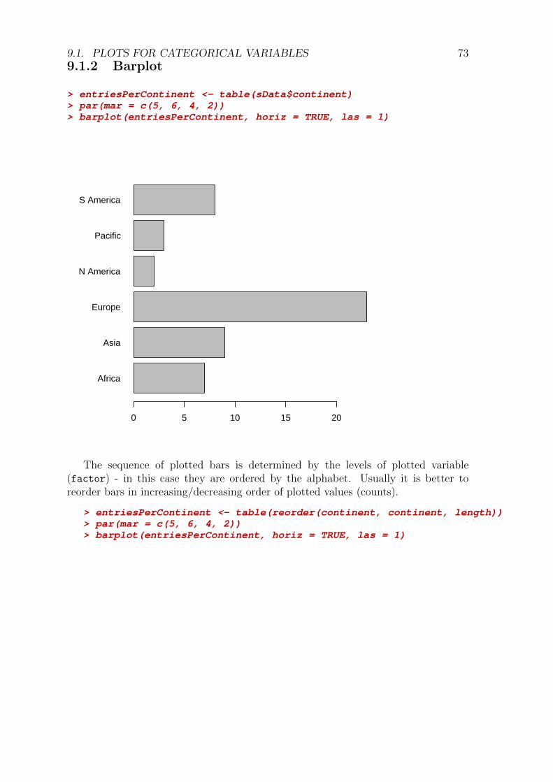
9.1. PLOTS FOR CATEGORICAL VARIABLES 739.1.2 Barplot
> entriesPerContinent <- table(sData$continent)> par(mar = c(5, 6, 4, 2))> barplot(entriesPerContinent, horiz = TRUE, las = 1)
Africa
Asia
Europe
N America
Pacific
S America
0 5 10 15 20
The sequence of plotted bars is determined by the levels of plotted variable(factor) - in this case they are ordered by the alphabet. Usually it is better toreorder bars in increasing/decreasing order of plotted values (counts).
> entriesPerContinent <- table(reorder(continent, continent, length))> par(mar = c(5, 6, 4, 2))> barplot(entriesPerContinent, horiz = TRUE, las = 1)

74 CHAPTER 9. PLOTTING
N America
Pacific
Africa
S America
Asia
Europe
0 5 10 15 20
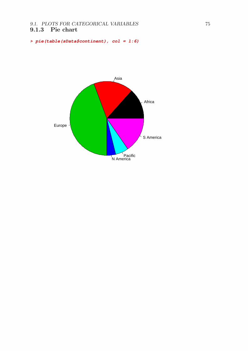
9.1. PLOTS FOR CATEGORICAL VARIABLES 759.1.3 Pie chart
> pie(table(sData$continent), col = 1:6)
Africa
Asia
Europe
N AmericaPacific
S America

76 CHAPTER 9. PLOTTING9.2 Plots for numerical variables
9.2.1 Histogram
> hist(lifeExpec, col = "lightblue")
Histogram of lifeExpec
lifeExpec
Fre
quen
cy
40 50 60 70 80
05
1015
2025
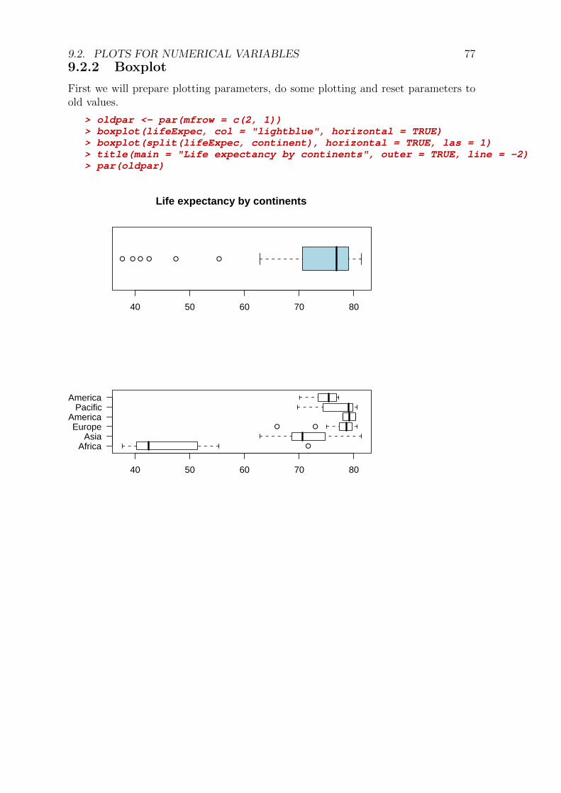
9.2. PLOTS FOR NUMERICAL VARIABLES 779.2.2 Boxplot
First we will prepare plotting parameters, do some plotting and reset parameters toold values.
> oldpar <- par(mfrow = c(2, 1))> boxplot(lifeExpec, col = "lightblue", horizontal = TRUE)> boxplot(split(lifeExpec, continent), horizontal = TRUE, las = 1)> title(main = "Life expectancy by continents", outer = TRUE, line = -2)> par(oldpar)
● ●● ●●●
40 50 60 70 80
●
●●
AfricaAsia
EuropeN America
PacificS America
40 50 60 70 80
Life expectancy by continents

78 CHAPTER 9. PLOTTING9.2.3 Scatterplot
> plot(tvSets, internetUsers)
●●
●
●
●
●
●
●
●
●
●
●
●●
●
●
●
●
●
●
●
●
●
●
●
●
●
●
●
●
●
●
●
●
●
●
●
●
●
●
●
●
●
●
●
●●
0 200 400 600
010
020
030
040
050
0
tvSets
inte
rnet
Use
rs
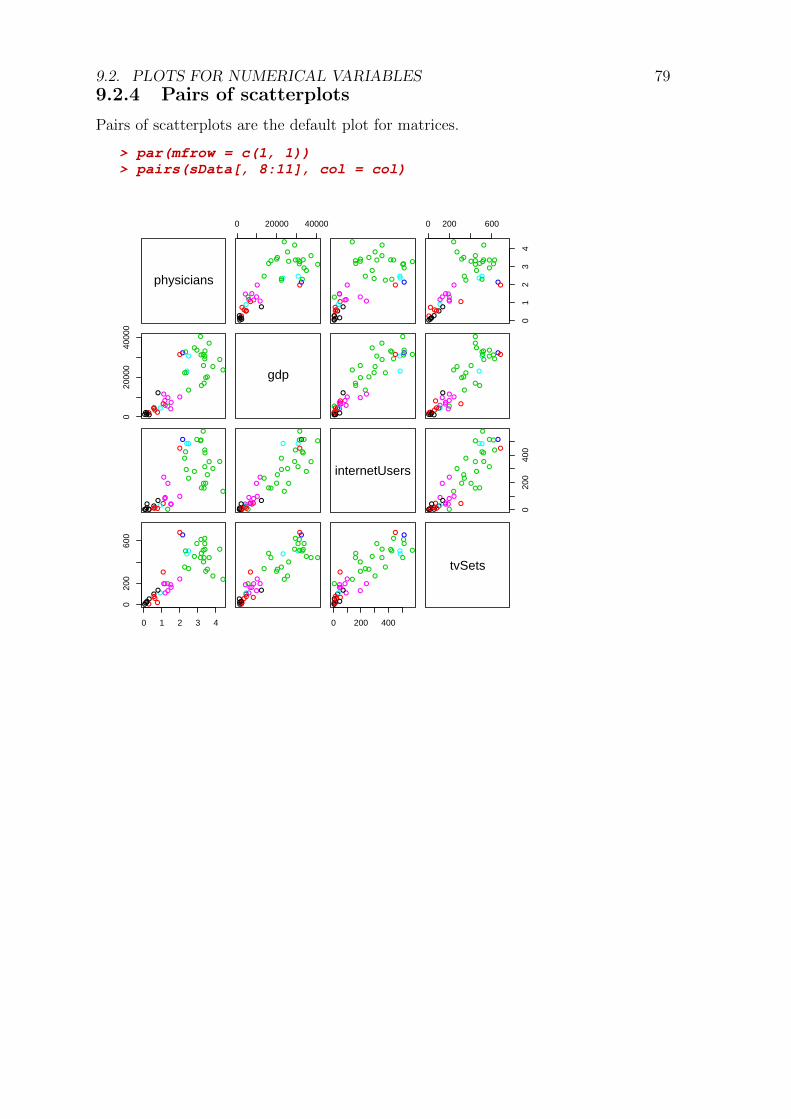
9.2. PLOTS FOR NUMERICAL VARIABLES 799.2.4 Pairs of scatterplots
Pairs of scatterplots are the default plot for matrices.
> par(mfrow = c(1, 1))> pairs(sData[, 8:11], col = col)
physicians
0 20000 40000
●
●
●
●
●
●
●
●●●
●
●
●
●
●
●●●
●
●
●
●
●
●
●
●
●
●
●
●
●
●
●
●●
●
●●
●
●
●
●
●●
●
●
●
●
●
●
●
●
●
●●●
●
●
●
●
●
●● ●
●
●
●
●
●
●
●
●
●
●
●
●
●
●
●
●●
●
●●
●
●
●
●
●●
●
●
0 200 600
01
23
4
●
●
●
●
●
●
●
● ●●
●
●
●
●
●● ●
●
●
●
●
●
●
●
●
●
●
●
●
●
●
●
●●
●
●●
●
●
●
●
●●
●
●
020
000
4000
0
●
●
●●
●
●
●
●
●●
●●
●
●●
●●●
●
●
●
●
●
●
●●
●
●
●
●
●
●
●
●●
●
●
●
●
●
●
●
●
●
●
●
gdp
●
●
●●
●
●
●
●
●●
●●
●
●●
●●●
●
●
●
●
●
●
●
●●
●
●
●
●
●
●
●
●●
●
●
●
●
●
●
●
●
●
●
●
●
●
●
●●
●
●
●
●
●●
●
●
●●
●●●
●
●
●
●
●
●
●
●●
●
●
●
●
●
●
●
●●
●
●
●
●
●
●
●
●
●
●
●
●
●●
●
●
●
●
●
●
●
●
●●
●
●●
●
●
●
●
●
●
●
●●
●
●
●
●
●
●
●
●
●●
●
●●
●
●
●
●
●
●
●
●
●●●
●
●
●
●
●
●
●
●
●●
●
●●
●
●
●
●
●
●
●●
●●
●
●
●
●
●
●
●
●
●●
●
●●
●
●
●
●
●
●
●
●
●●
internetUsers
020
040
0
●●
●
●
●
●
●
●
●
●
●
●
●●
●
●
●
●
●
●
●●
●●
●
●
●
●
●
●
●
●
●●
●
●●
●
●
●
●
●
●
●
●
●●
0 1 2 3 4
020
060
0
●
●
● ●
●
●
●
●
●
●
●
●
●
●
●●●
●
●
●
●
●
●
●
●
●
●
●
●
●
●
●
●●
●●
●
●
●
●
●
●
●
●
●
●
●
● ●
●
●
●
●
●
●
●
●
●
●
●●
●
●
●
●
● ●
●
●
●
●
●
●
●
●
●
●
●
●●
●●
●
●
●
●
●
●
●
●
●
●
0 200 400
●
●
●●
●
●
●
●
●
●
●
●
●
●
●●
●
●
●
●
●●
●
●
●
●
●
●
●
●
●
●
●
●●
●●
●
●
●
●
●
●
●
●
●
●
tvSets

80 CHAPTER 9. PLOTTING9.2.5 Three dimensional plots
Basic 3d plotting commands are shown below, for additional possibilities see con-tributed packages.
Density plot: image and contours
> x <- (-10:10)> y <- x> z <- outer(x^2,y^2,"+") # perform add on all pairs> image(z)> contour(z,add=TRUE)
0.0 0.2 0.4 0.6 0.8 1.0
0.0
0.2
0.4
0.6
0.8
1.0
20
40
60
80
100
120
120
120
120
140
140
140
140
160
160
160
160
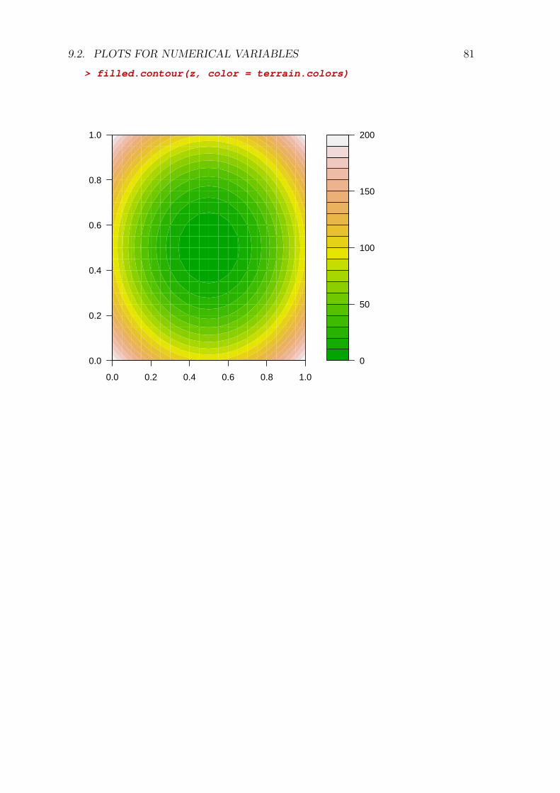
9.2. PLOTS FOR NUMERICAL VARIABLES 81
> filled.contour(z, color = terrain.colors)
0
50
100
150
200
0.0 0.2 0.4 0.6 0.8 1.0
0.0
0.2
0.4
0.6
0.8
1.0

82 CHAPTER 9. PLOTTINGPerpective plot
> persp(x, y, z, col = "lightblue", shade = 0.25)
x
y
z
9.3 High level plotting commands
In previous section we used one of high level plotting commands. The most importantfeature of them is that they set up a new graph with new coordinate system.
We will try some graphs with variables from sData:
> names(sData)
[1] "country" "continent" "infantMort" "lifeExpec"[5] "population" "birthRate" "nPhysicians" "physicians"[9] "gdp" "internetUsers" "tvSets"
> attach(sData)
The following object(s) are masked from sData ( position 3 ) :
birthRate continent country gdp infantMort internetUsers lifeExpec nPhysicians physicians population tvSets
> col = as.numeric(as.factor(continent))

9.3. HIGH LEVEL PLOTTING COMMANDS 83
> par(mfrow = c(2, 2))> plot(lifeExpec, col = col)> plot(birthRate, lifeExpec, col = col)> plot(continent, col = col)> plot(continent, lifeExpec, col = col)
●
●
●●
●
●
●●
●
●●●●●
●
●●●●
●●
●●
●●●
●
●
●●
●
●
●
●
●
●
●
●●
●
●●
●
●
●
●●
●
●●●
●
0 10 20 30 40 50
4050
6070
80
Index
lifeE
xpec
●
●
●●
●
●
●●
●
●●●
●●
●
●●●●
●●
●●
●●●
●
●
●●
●
●
●
●
●
●
●
●●
●
●●
●
●
●
●●
●
● ●●
●
10 20 30 40
4050
6070
80
birthRate
lifeE
xpec
Africa Europe Pacific
05
1015
20
●●
●
Africa Europe Pacific
4050
6070
80
> plot(~birthRate+lifeExpec+infantMort+gdp,col=col)

84 CHAPTER 9. PLOTTING
birthRate
40 50 60 70 80
●
●
●
●
●
●
●
●●
●
●
●●
●●
●●
●●
●
●
●
●●
●
●●
●
●
●
●
●
●
●
●
●●
●●● ●●
●
●
●
●●
●
●
●
●
●
●
●
●
●
●
●
●
●●
●
●
●●
●●
●●
●●
●
●
●
●●
●
●●
●
●
●
●
●
●
●
●
●●
●●●●●
●
●
●
●●
●
●
●
●
●
0 20000 40000
1020
3040
●
●
●
●
●
●
●
●●
●
●
●●
●●
●●
●●
●
●
●
●●
●
● ●
●
●
●
●
●
●
●
●●
● ●●●
●
●
●
● ●●
●
●
4050
6070
80 ●
●
●●
●
●
●●
●
●●●
● ●
●
●●●●
●●
●●
●●●
●
●
●●
●
●
●
●
●
●
●
●●
●
●●
●
●
●
●●
●
● ●●
●
lifeExpec
●
●
●●
●
●
●●
●
●●●● ●
●
●●●●
●●
●●
●●●
●
●
●●
●
●
●
●
●
●
●
●●
●
●●
●
●
●
●●
●
●●●
●
●
●
● ●
●
●
●●
●
● ●●
●●
●
●●●●
●●
●●
●● ●
●
●
●
●
●
●
●
●
●
●
●●
●●
●
●
●
● ●●
●
●
●
●
●●
●
●
● ●●
●●●●
●●
●●●●
●
●
●●
● ●●●
●
●●
●
●
●
●
●
●●
●●●●●
●
●
●
●●
●
● ●●
●
●
●
●●
●
●
●●●
●●●●
●●
●●●●
●
●
●●
●●●●
●
●●
●
●
●
●
●
●●
●●● ●●
●
●
●
●●
●
●●●
●
infantMort
050
100
150
●
●
● ●
●
●
●●●
● ●● ●
●●
●●●●
●
●
● ●
●● ● ●
●
●
●
●
●
●
●
●●
● ●● ●
●
●
●
● ●●
●
●
10 20 30 40
020
000
4000
0
●
●
●●
●
●
●
●
●●
●●
●
●●
●●●
●
●
●
●
●
●
●
●●
●
●
●
●
●
●
●
●●
●
●
●
●
●
●
●
●
●
●
●
●
●
●
●●
●
●
●
●
●●
●●
●
●●
●●●
●
●
●
●
●
●
●
●●
●
●
●
●
●
●
●
●●
●
●
●
●
●
●
●
●
●
●
●
●
0 50 100 150
●
●
●●
●
●
●
●
●●
●●
●
●●
●●●
●
●
●
●
●
●
●
●●
●
●
●
●
●
●
●
●●
●
●
●
●
●
●
●
●
●
●
●
●
gdp
9.4. LOW LEVEL COMMANDS 859.4 Low level commands
Low level commands add points, lines, texts, segments, and legend to existing plot.
� points
� lines
� segments
� text
� mtext
� abline
� rug
� legend
To show the use of plotting commands, we will simulate the situation in which xand y are normally distributed: X ∼ N(10, 1) and Y = a+ bX + ε where ε ∼ N(0, 3)and make a customized graph.

86 CHAPTER 9. PLOTTING
> set.seed(1357)> n <- 30> a <- 10> b <- 2> x <- rnorm(n,10)> y <- a+b*x+rnorm(n,0,3)> ##> plot(x,y,xlim=c(7,12),ylim=c(20,40))> points(mean(x),mean(y),pch=16,col="red",cex=2) # add centroid point> range(x)
[1] 7.301743 11.766331
> range(y)
[1] 21.12839 35.66525
> points(range(x),range(y),pch=16,col="blue") # mark extreme two points> lines(range(x),a+b*range(x)) # add model line> text(max(x),max(y)+2,"maximum")> mtext("right justified text in margin 4",4,cex=0.75,adj=1)> ab <- lsfit(x,y)> abline(ab$coeff,col=6,lwd=3) # add regression line> abline(v=8) # vertical line at 8> aEst <- ab$coeff[1]> bEst <- ab$coeff[2]> text(8,38,paste("a =",round(aEst,1))) # centred text> text(8,36,paste("b = ",round(bEst,1)),adj=0) # left justified> rug(x,side=1,col="blue")> rug(y,side=4,col=6)> ## residuals> yEst <- aEst + bEst *x> points(x,yEst,col=4)> segments (x, y, x, yEst,col=2)> abline(h=seq(20,40,5),col="grey",lty=3) # add grey gridlines> legend(9,40,col=c("black","magenta","red"),+ lwd=c(1,3,1),+ legend=c("model","regression","residual"),+ cex=0.7)
●
●
●
●
●●
●
●
●●
●●
●
●
●
●
●
●
●●
●
●
●
●
●
●
●
●
●
●
7 8 9 10 11 12
2025
3035
40
x
y
●
●
●
maximum
right
just
ified
text
in m
argi
n 4
a = 7.6
b = 2.1
●
●
●
●
●
●
●
●
●
●
●
●
●
●
●
●
●
●
●
●
●
●
●
●
●
●
●
●
●
●
modelregressionresidual
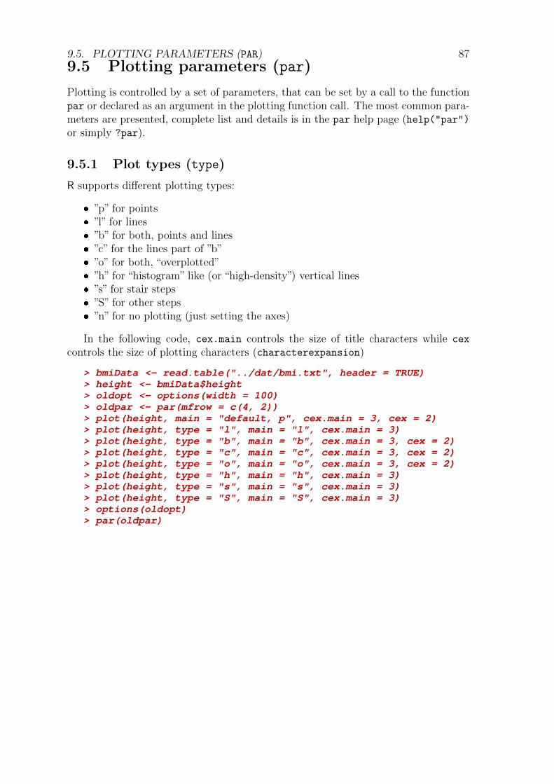
9.5. PLOTTING PARAMETERS (PAR) 879.5 Plotting parameters (par)
Plotting is controlled by a set of parameters, that can be set by a call to the functionpar or declared as an argument in the plotting function call. The most common para-meters are presented, complete list and details is in the par help page (help("par")or simply ?par).
9.5.1 Plot types (type)
R supports different plotting types:
� ”p” for points� ”l” for lines� ”b” for both, points and lines� ”c” for the lines part of ”b”� ”o” for both, “overplotted”� ”h” for “histogram” like (or “high-density”) vertical lines� ”s” for stair steps� ”S” for other steps� ”n” for no plotting (just setting the axes)
In the following code, cex.main controls the size of title characters while cex
controls the size of plotting characters (characterexpansion)
> bmiData <- read.table("../dat/bmi.txt", header = TRUE)> height <- bmiData$height> oldopt <- options(width = 100)> oldpar <- par(mfrow = c(4, 2))> plot(height, main = "default, p", cex.main = 3, cex = 2)> plot(height, type = "l", main = "l", cex.main = 3)> plot(height, type = "b", main = "b", cex.main = 3, cex = 2)> plot(height, type = "c", main = "c", cex.main = 3, cex = 2)> plot(height, type = "o", main = "o", cex.main = 3, cex = 2)> plot(height, type = "h", main = "h", cex.main = 3)> plot(height, type = "s", main = "s", cex.main = 3)> plot(height, type = "S", main = "S", cex.main = 3)> options(oldopt)> par(oldpar)

88 CHAPTER 9. PLOTTING
●
●
●
●●
●
●
●
●
●
●
●
●
●●
●
●
●
●
●
●
●
●
●●
●
●
●
●●
●
●
●●
●●
●
●●
●●
●
●
●
●
0 10 20 30 40
1.6
1.7
1.8
1.9
default, p
Index
heig
ht
0 10 20 30 40
1.6
1.7
1.8
1.9
l
Index
heig
ht
●
●
●
●●
●
●
●
●
●
●
●
●
●●
●
●
●
●
●
●
●
●
●●
●
●
●
●●
●
●
●●
●●
●
●●
●●
●
●
●
●
0 10 20 30 40
1.6
1.7
1.8
1.9
b
Index
heig
ht
0 10 20 30 40
1.6
1.7
1.8
1.9
c
Index
heig
ht
●
●
●
●●
●
●
●
●
●
●
●
●
●●
●
●
●
●
●
●
●
●
●●
●
●
●
●●
●
●
●●
●●
●
●●
●●
●
●
●
●
0 10 20 30 40
1.6
1.7
1.8
1.9
o
Index
heig
ht
0 10 20 30 40
1.6
1.7
1.8
1.9
h
Index
heig
ht
0 10 20 30 40
1.6
1.7
1.8
1.9
s
Index
heig
ht
0 10 20 30 40
1.6
1.7
1.8
1.9
S
Index
heig
ht

9.5. PLOTTING PARAMETERS (PAR) 899.5.2 Line type and width (lty and lwd)
> show.lty()
lwd lty0.5 1
1 21.5 3
2 42.5 5
3 63.5 1
4 24.5 3
5 45.5 5
6 66.5 1
7 27.5 3
8 48.5 5
9 69.5 110 2
10.5 311 4
11.5 512 6
12.5 113 2
13.5 314 4
14.5 515 6
15.5 116 2
col cex0 0
1 0.2
2 0.4
3 0.6
4 0.8
5 1
6 1.2
7 1.4
8 1.69 1.8
10 211 2.212 2.413 2.614 2.815 316 3.2
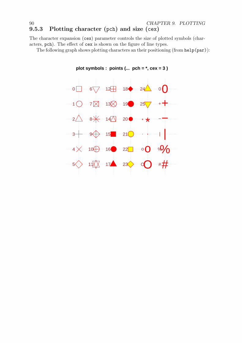
90 CHAPTER 9. PLOTTING9.5.3 Plotting character (pch) and size (cex)
The character expansion (cex) parameter controls the size of plotted symbols (char-acters, pch). The effect of cex is shown on the figure of line types.
The following graph shows plotting characters an their positioning (from help(par)):
plot symbols : points (... pch = *, cex = 3 )
0
●1
2
3
4
5
6
7
8
9
●10
11
12
●13
14
15
●16
17
18
●19
●20
●21
22
23
24
25
**
.
oo
OO
00
++
−−
||
%%
##

9.5. PLOTTING PARAMETERS (PAR) 91Plotting characters, listed by number:
> show.pch()
0
●1 2 3 4 5 6 7 8 9
●10 11 12
●13 14 15
●16 17 18
●19
●
20
●21 22 23 24 25 26 27 28 29 30 31
32
!33
"34
#35
$36
%37
&38
'39
(40
)41
*42
+43
,44
−45 46
/47
048
149
250
351
452
553
654
755
856
957
:58
;59
<60
=61
>62
?63
@64
A65
B66
C67
D68
E69
F70
G71
H72
I73
J74
K75
L76
M77
N78
O79
P80
Q81
R82
S83
T84
U85
V86
W87
X88
Y89
Z90
[91
\92
]93 9̂4
_95
9̀6
a97
b98
c99
d100
e101
f102
g103
h104
i105
j106
k107
l108
m109
n110
o111
p112
q113
r114
s115
t116
u117
v118
w119
x120
y121
z122
{123
|124
}125
~126
•127
€128
.129
‚130
.131
„132
…133
†134
‡135
.136
‰137
Š138
‹139
..140
..141
Ž142
..143
.144
‘145
’146
“147
”148
•149
–150
—151
.152
™153
š154
›155
..156
..157
ž158
..159
160
..161
..162
..163
¤164
..165
¦166
§167 1̈68
©169
..170
«171
¬172
173
®174
..175
°176
±177
..178
..179 1́80
µ181
¶182
·183
¸184
..185
..186
»187
..188
..189
..190
..191
..192
Á193
Â194
..195
Ä196
..197
..198
Ç199
..200
É201
..202
Ë203
..204
Í205
Î206
..207
..208
..209
..210
Ó211
Ô212
..213
Ö214
×215
..216
..217
Ú218
..219
Ü220
Ý221
..222
ß223
..224
á225
â226
..227
ä228
..229
..230
ç231
..232
é233
..234
ë235
..236
í237
î238
..239
..240
..241
..242
ó243
ô244
..245
ö246
÷247
..248
..249
ú250
..251
ü252
ý253
..254
..255
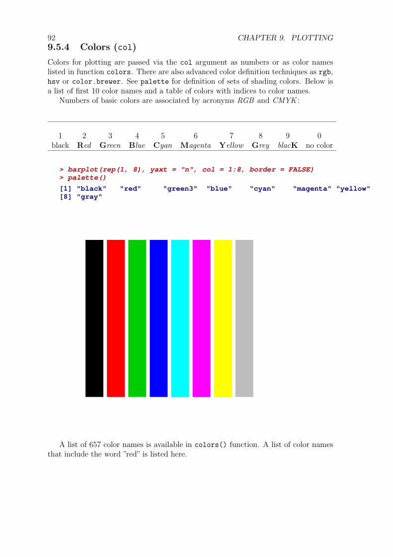
92 CHAPTER 9. PLOTTING9.5.4 Colors (col)
Colors for plotting are passed via the col argument as numbers or as color nameslisted in function colors. There are also advanced color definition techniques as rgb,hsv or color.brewer. See palette for definition of sets of shading colors. Below isa list of first 10 color names and a table of colors with indices to color names.
Numbers of basic colors are associated by acronyms RGB and CMYK :
1 2 3 4 5 6 7 8 9 0black Red Green Blue Cyan Magenta Yellow Grey blacK no color
> barplot(rep(1, 8), yaxt = "n", col = 1:8, border = FALSE)> palette()
[1] "black" "red" "green3" "blue" "cyan" "magenta" "yellow"[8] "gray"
A list of 657 color names is available in colors() function. A list of color namesthat include the word ”red” is listed here.

9.5. PLOTTING PARAMETERS (PAR) 93
> colors()[grep("red", colors())]
[1] "darkred" "indianred" "indianred1" "indianred2"[5] "indianred3" "indianred4" "mediumvioletred" "orangered"[9] "orangered1" "orangered2" "orangered3" "orangered4"[13] "palevioletred" "palevioletred1" "palevioletred2" "palevioletred3"[17] "palevioletred4" "red" "red1" "red2"[21] "red3" "red4" "violetred" "violetred1"[25] "violetred2" "violetred3" "violetred4"
Colors and their indices are plotted below:
> show.colors(cex = 7)
1
2
3
4
5
6
7
8
9
10
11
12
13
14
15
16
17
18
19
20
21
22
23
24
25
26
27
28
29
30
31
32
33
34
35
36
37
38
39
40
41
42
43
44
45
46
47
48
49
50
51
52
53
54
55
56
57
58
59
60
61
62
63
64
65
66
67
68
69
70
71
72
73
74
75
76
77
78
79
80
81
82
83
84
85
86
87
88
89
90
91
92
93
94
95
96
97
98
99
100
101
102
103
104
105
106
107
108
109
110
111
112
113
114
115
116
117
118
119
120
121
122
123
124
125
126
127
128
129
130
131
132
133
134
135
136
137
138
139
140
141
142
143
144
145
146
147
148
149
150
151
152
153
154
155
156
157
158
159
160
161
162
163
164
165
166
167
168
169
170
171
172
173
174
175
176
177
178
179
180
181
182
183
184
185
186
187
188
189
190
191
192
193
194
195
196
197
198
199
200
201
202
203
204
205
206
207
208
209
210
211
212
213
214
215
216
217
218
219
220
221
222
223
224
225
226
227
228
229
230
231
232
233
234
235
236
237
238
239
240
241
242
243
244
245
246
247
248
249
250
251
252
253
254
255
256
257
258
259
260
261
262
263
264
265
266
267
268
269
270
271
272
273
274
275
276
277
278
279
280
281
282
283
284
285
286
287
288
289
290
291
292
293
294
295
296
297
298
299
300
301
302
303
304
305
306
307
308
309
310
311
312
313
314
315
316
317
318
319
320
321
322
323
324
325
326
327
328
329
330
331
332
333
334
335
336
337
338
339
340
341
342
343
344
345
346
347
348
349
350
351
352
353
354
355
356
357
358
359
360
361
362
363
364
365
366
367
368
369
370
371
372
373
374
375
376
377
378
379
380
381
382
383
384
385
386
387
388
389
390
391
392
393
394
395
396
397
398
399
400
401
402
403
404
405
406
407
408
409
410
411
412
413
414
415
416
417
418
419
420
421
422
423
424
425
426
427
428
429
430
431
432
433
434
435
436
437
438
439
440
441
442
443
444
445
446
447
448
449
450
451
452
453
454
455
456
457
458
459
460
461
462
463
464
465
466
467
468
469
470
471
472
473
474
475
476
477
478
479
480
481
482
483
484
485
486
487
488
489
490
491
492
493
494
495
496
497
498
499
500
501
502
503
504
505
506
507
508
509
510
511
512
513
514
515
516
517
518
519
520
521
522
523
524
525
526
527
528
529
530
531
532
533
534
535
536
537
538
539
540
541
542
543
544
545
546
547
548
549
550
551
552
553
554
555
556
557
558
559
560
561
562
563
564
565
566
567
568
569
570
571
572
573
574
575
576
577
578
579
580
581
582
583
584
585
586
587
588
589
590
591
592
593
594
595
596
597
598
599
600
601
602
603
604
605
606
607
608
609
610
611
612
613
614
615
616
617
618
619
620
621
622
623
624
625
626
627
628
629
630
631
632
633
634
635
636
637
638
639
640
641
642
643
644
645
646
647
648
649
650
651
652
653
654
655
656
657
1
2
3
4
5
6
7
8
9
10
11
12
13
14
15
16
17
18
19
9.5.5 Plot and axis labels
To overrule the default axis labeling by the variable names, xlab and ylab can beused. To put a title and subtitle use arguments main and sub. You can use \n tosplit the title into lines.

94 CHAPTER 9. PLOTTING
> attach(bmiData)
The following object(s) are masked _by_ .GlobalEnv :
height
> plot(height, weight,+ xlab = "Body height [m]",+ ylab = "Body weight [kg]",+ main = "Relation of height and weight",+ sub = "(labeled plot)",+ col.lab = "red",+ col.main = "blue",+ col.sub = "orange")> detach()
●
●
●
● ●
●
●
●
●
●
●
●
●
●
●
●
●
●
●
●
●●
●
●
●
●
●
●
●●
●●
●
●●
●
●
●●
●
●
●
●
●
●
1.6 1.7 1.8 1.9
5060
7080
90
Relation of height and weight
(labeled plot)Body height [m]
Bod
y w
eigh
t [kg
]
Function title(...) can be used for labeling of an existing plot. In addition tocol and cex for plot color and plotting character size (expansion), dotted arguments(as in the preceding example) for labels, main and sub title are available e. g. col.laband cex.lab.
9.5.6 Axis limits
By default, data range is used for axis limits. To override the default, argumentsxlim and ylim can be used:

9.5. PLOTTING PARAMETERS (PAR) 95
> attach (bmiData)
The following object(s) are masked _by_ .GlobalEnv :
height
> plot(height, weight,+ xlim = c(1, 2),+ ylim = c(0, 100),+ xlab = "Body height [m]",+ ylab = "Body weight [kg]"+ )> detach ()
●
●
●
● ●
●
●
●
●
●
●
●
●
●
●
●●
●
●
●
● ●
●
●
●
●
●
●●●
●●●
● ●
●
●
●●
●●
●●
●
●
1.0 1.2 1.4 1.6 1.8 2.0
020
4060
8010
0
Body height [m]
Bod
y w
eigh
t [kg
]

96 CHAPTER 9. PLOTTING

9.6. TUNING THE GRAPH 979.6 Tuning the graph
> ind <- rev(order(sData$population))> X <- sData[ind, ]> attach(X)
The following object(s) are masked from sData ( position 3 ) :
birthRate continent country gdp infantMort internetUsers lifeExpec nPhysicians physicians population tvSets
The following object(s) are masked from sData ( position 4 ) :
birthRate continent country gdp infantMort internetUsers lifeExpec nPhysicians physicians population tvSets
> oldpar <- par(mfrow = c(2, 2))> cex <- 5 * sqrt(population/10^9)> col <- as.numeric(continent)> plot(gdp, infantMort, cex = cex, col = col)> bg <- col> ind <- rev(order(population))> plot(gdp, infantMort, cex = cex, pch = 21, bg = bg, col = 1)> plot(gdp, infantMort, cex = 1, pch = 21, bg = bg, col = 1, log = "xy")> plot(gdp, infantMort, cex = cex, pch = 21, bg = bg, col = 1,+ log = "xy")> if (interactive()) identify(gdp, infantMort, log = "xy", country)> par(oldpar)> detach()
●
●●
●
●●
●
●●
● ●●
●
●●
●
●
●●●
●
●●
●●
●
●
●●●●
● ● ●●
●●
● ●
●● ●
●●
●
●
0 10000 30000
050
100
150
gdp
infa
ntM
ort
●
●●
●
●●
●
●●
● ●●
●
●●
●
●
●●●
●
●●
●●
●
●
●●●●
● ● ●●
●●
● ●
●● ●
●●
●
●
0 10000 30000
050
100
150
gdp
infa
ntM
ort
●
●●
●●
●
●
●
●
●●
●●
●
●
●
●
●
●
●
●●
●
●
●
●●
●
●
●●●
●
●
●●
●
●
●
● ●
●
● ●
●●
●
●
1000 5000 20000
520
5020
0
gdp
infa
ntM
ort
●
●●●
●
●
●
●●
●●●
●
●
●
●
●
●
●●
●
●
●
●
●
●
●
●●
●
●
●
● ●
●
●
●
● ●
●
●●
●
●
●
●
1000 5000 20000
520
5020
0
gdp
infa
ntM
ort

98 CHAPTER 9. PLOTTING
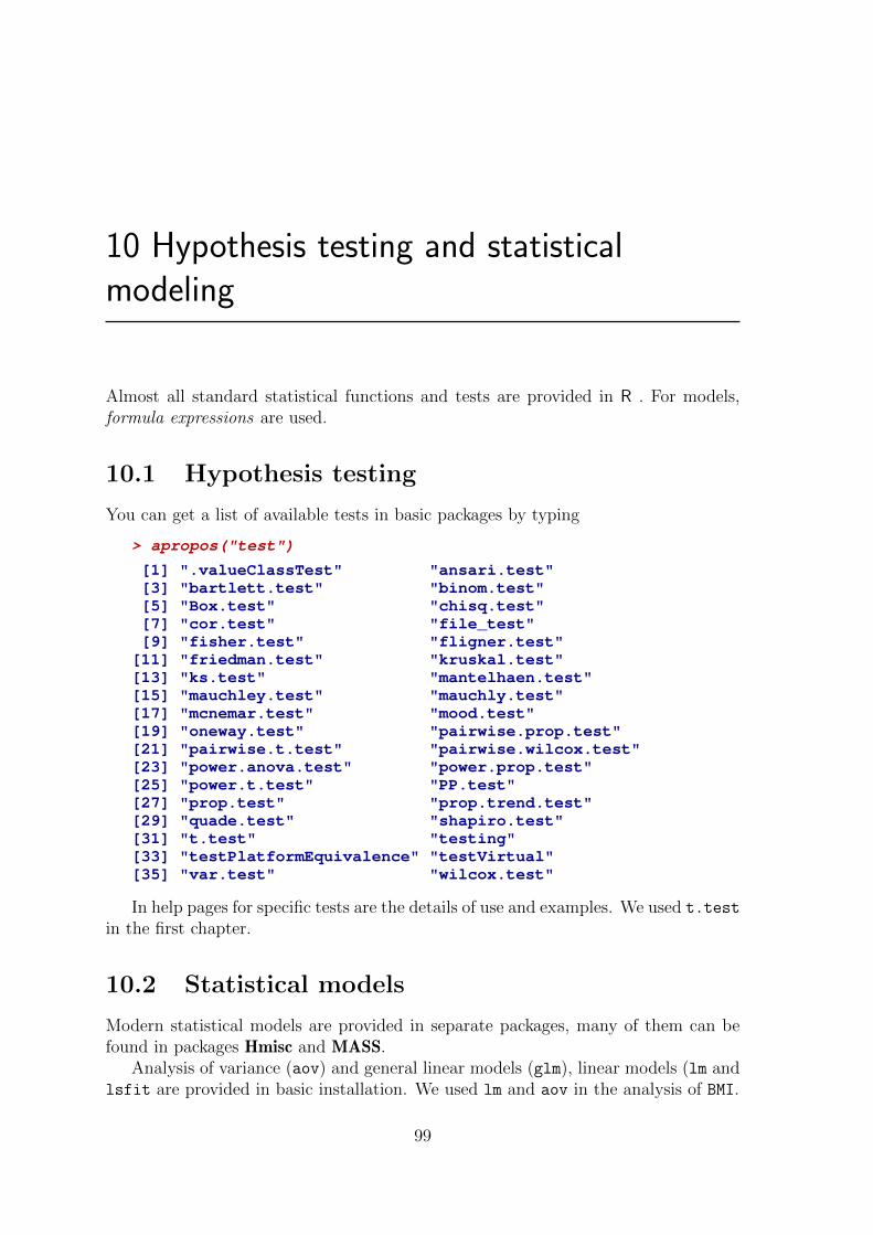
10 Hypothesis testing and statisticalmodeling
Almost all standard statistical functions and tests are provided in R . For models,formula expressions are used.
10.1 Hypothesis testing
You can get a list of available tests in basic packages by typing
> apropos("test")
[1] ".valueClassTest" "ansari.test"[3] "bartlett.test" "binom.test"[5] "Box.test" "chisq.test"[7] "cor.test" "file_test"[9] "fisher.test" "fligner.test"[11] "friedman.test" "kruskal.test"[13] "ks.test" "mantelhaen.test"[15] "mauchley.test" "mauchly.test"[17] "mcnemar.test" "mood.test"[19] "oneway.test" "pairwise.prop.test"[21] "pairwise.t.test" "pairwise.wilcox.test"[23] "power.anova.test" "power.prop.test"[25] "power.t.test" "PP.test"[27] "prop.test" "prop.trend.test"[29] "quade.test" "shapiro.test"[31] "t.test" "testing"[33] "testPlatformEquivalence" "testVirtual"[35] "var.test" "wilcox.test"
In help pages for specific tests are the details of use and examples. We used t.test
in the first chapter.
10.2 Statistical models
Modern statistical models are provided in separate packages, many of them can befound in packages Hmisc and MASS.
Analysis of variance (aov) and general linear models (glm), linear models (lm andlsfit are provided in basic installation. We used lm and aov in the analysis of BMI.
99

100 CHAPTER 10. HYPOTHESIS TESTING AND STATISTICAL MODELING
> dimnames(sData)[[1]] <- sData$country> attach(sData)> R <- cor(sData[, -(1:2)], use = "pairwise.complete")> round(R, 2)
infantMort lifeExpec population birthRate nPhysicians physiciansinfantMort 1.00 -0.88 0.06 0.87 -0.06 -0.69lifeExpec -0.88 1.00 -0.05 -0.80 0.08 0.71population 0.06 -0.05 1.00 0.05 0.93 -0.26birthRate 0.87 -0.80 0.05 1.00 -0.11 -0.80nPhysicians -0.06 0.08 0.93 -0.11 1.00 -0.08physicians -0.69 0.71 -0.26 -0.80 -0.08 1.00gdp -0.62 0.63 -0.24 -0.74 -0.09 0.83internetUsers -0.58 0.59 -0.25 -0.68 -0.12 0.69tvSets -0.64 0.64 -0.08 -0.77 0.06 0.77
gdp internetUsers tvSetsinfantMort -0.62 -0.58 -0.64lifeExpec 0.63 0.59 0.64population -0.24 -0.25 -0.08birthRate -0.74 -0.68 -0.77nPhysicians -0.09 -0.12 0.06physicians 0.83 0.69 0.77gdp 1.00 0.92 0.90internetUsers 0.92 1.00 0.89tvSets 0.90 0.89 1.00
> lmFit = lm(infantMort ~ population + gdp + nPhysicians)> lmFit
Call:lm(formula = infantMort ~ population + gdp + nPhysicians)
Coefficients:(Intercept) population gdp nPhysicians5.535e+01 1.873e-08 -1.704e-03 -3.718e-05
> summary(lmFit)
Call:lm(formula = infantMort ~ population + gdp + nPhysicians)
Residuals:Min 1Q Median 3Q Max
-29.234 -15.919 -1.932 7.323 132.632
Coefficients:Estimate Std. Error t value Pr(>|t|)
(Intercept) 5.535e+01 7.798e+00 7.097 1.06e-08 ***population 1.873e-08 4.952e-08 0.378 0.707gdp -1.704e-03 3.738e-04 -4.559 4.39e-05 ***nPhysicians -3.718e-05 5.416e-05 -0.686 0.496---Signif. codes: 0 '***' 0.001 '**' 0.01 '*' 0.05 '.' 0.1 ' ' 1
Residual standard error: 27.79 on 42 degrees of freedom(6 observations deleted due to missingness)
Multiple R-squared: 0.4045, Adjusted R-squared: 0.362F-statistic: 9.509 on 3 and 42 DF, p-value: 6.474e-05
> pairs(infantMort ~ population + gdp + nPhysicians)> detach()
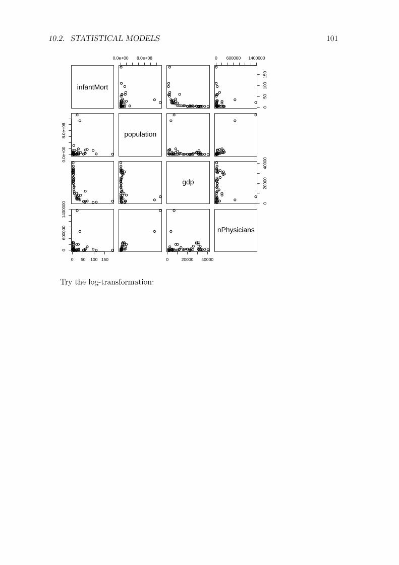
10.2. STATISTICAL MODELS 101
infantMort
0.0e+00 8.0e+08
●
●
●●
●
●
●●●
●●●●
●●
●●●●
●
●
●●
●●●●
●
●●
●
●
●
●
●
●●
●●●●●
●
●
●
●●
●
● ●●
●
●
●
● ●
●
●
●●●
● ●● ●
●●
●●●●
●
●
● ●
●● ● ●
●
●
●
●
●
●
●
●●
● ●● ●
●
●
●
● ●●
●
●
0 600000 1400000
050
100
150
●
●
●●
●
●
●●●
●●●●
●●
● ●●●
●
●
●
●● ●●
●
●
●
●
●
●
●
●●
●●●●
●
●
●
●● ●
●
0.0e
+00
8.0e
+08
● ●●●
●●
●●
●
●●●● ●●
●●●● ●●
●
●●●●●
●●●
●●
●
●
●
● ●●●
●
●● ●● ●●● ●●
●
● ●
population
●● ● ●
● ●
●●
●
● ●● ●●●
●●●
●● ●
●
●●●
●●
●●
● ●
●
●
●
●● ● ●● ●● ●● ● ●●●● ●●●●
● ●
●●
●
●●●●●●●
●●●●●
●
●●●●
●●
●●
●
●
●
●●●●●●● ●●●●●
●
●
●
●●
●
●
●
●
●●
●●
●
●●
●●●
●
●
●
●
●
●
●
●●
●
●
●
●
●
●
●
●●
●
●
●
●
●
●
●
●
●
●
●
●
●
●
●●
●
●
●
●
●●
●●
●
●●
●●●
●
●
●
●
●
●
●
●●
●
●
●
●
●
●
●
●●
●
●
●
●
●
●
●
●
●
●
●
●
gdp
020
000
4000
0
●
●
●●
●
●
●
●
●●
●●
●
●●
● ●●
●
●
●
●
●
●
●●
●
●
●
●
●
●
●
●●
●
●
●
●
●
●
●
●
●
●
●
0 50 100 150
060
0000
1400
000
● ●●● ●
●
●●
●
●●●● ●●●
●●
● ●●
●
●●
●●
●
●
●● ●●●
● ●●●●● ●●
●●●●
● ●●●● ●
●
●●
●
●●●●●●●
●●
●●●
●
●●
●●
●
●
●● ●●●
●●●
●●●●●
●●●●
●
0 20000 40000
●●● ●●
●
●●
●
● ●● ●●● ●
●●
●● ●
●
●●
● ●
●
●
● ●● ●●
●●●
●● ●●●
● ● ●●
●
nPhysicians
Try the log-transformation:

102 CHAPTER 10. HYPOTHESIS TESTING AND STATISTICAL MODELING
> lsData <- log(sData[, -(1:2)])> attach(lsData)> R <- cor(lsData[, -(1:2)], use = "pairwise.complete")> round(R, 2)
population birthRate nPhysicians physicians gdp internetUserspopulation 1.00 0.19 0.75 -0.28 -0.35 -0.33birthRate 0.19 1.00 -0.38 -0.87 -0.91 -0.84nPhysicians 0.75 -0.38 1.00 0.43 0.29 0.27physicians -0.28 -0.87 0.43 1.00 0.89 0.83gdp -0.35 -0.91 0.29 0.89 1.00 0.92internetUsers -0.33 -0.84 0.27 0.83 0.92 1.00tvSets -0.19 -0.87 0.42 0.91 0.89 0.88
tvSetspopulation -0.19birthRate -0.87nPhysicians 0.42physicians 0.91gdp 0.89internetUsers 0.88tvSets 1.00
> lmFit = lm(infantMort ~ population + gdp + nPhysicians)> lmFit
Call:lm(formula = infantMort ~ population + gdp + nPhysicians)
Coefficients:(Intercept) population gdp nPhysicians
6.5819 0.3045 -0.7109 -0.2557
> summary(lmFit)
Call:lm(formula = infantMort ~ population + gdp + nPhysicians)
Residuals:Min 1Q Median 3Q Max
-0.66421 -0.21695 -0.03618 0.14591 1.50142
Coefficients:Estimate Std. Error t value Pr(>|t|)
(Intercept) 6.5819 2.0763 3.170 0.00284 **population 0.3045 0.1236 2.463 0.01797 *gdp -0.7109 0.1232 -5.771 8.47e-07 ***nPhysicians -0.2557 0.1141 -2.241 0.03038 *---Signif. codes: 0 '***' 0.001 '**' 0.01 '*' 0.05 '.' 0.1 ' ' 1
Residual standard error: 0.3885 on 42 degrees of freedom(6 observations deleted due to missingness)
Multiple R-squared: 0.891, Adjusted R-squared: 0.8832F-statistic: 114.4 on 3 and 42 DF, p-value: < 2.2e-16
> pairs(infantMort ~ population + gdp + nPhysicians)

10.3. MULTIVARIATE ANALYSIS 103For some models, you can plot informative analytical graphs
> plot(lmFit)
10.3 Multivariate analysis
Complete set of functions and operators for linear algebra is provided and very effi-cient. Operator %*% is used for matrix multiplication and function eigen for eigen-value analysis.
All standard multivariate procedures are available.
> X <- sData[-which(is.na(sData), arr.ind = TRUE)[, 1], ]> PC <- prcomp(X[, -(1:2)], scale = TRUE)> PC
Standard deviations:[1] 2.3566503 1.4093063 0.8568253 0.5394988 0.4067815 0.3360706 0.2541269[8] 0.2316664 0.1954032
Rotation:PC1 PC2 PC3 PC4 PC5
infantMort 0.36055526 0.11772491 -0.507415576 0.24157403 -0.24082941lifeExpec -0.36046771 -0.12728796 0.444210090 -0.21332734 -0.67124972population 0.09287870 -0.67709770 -0.118413259 -0.02714552 -0.11503028birthRate 0.38909606 0.12747680 -0.218203284 -0.09280392 -0.62439138nPhysicians 0.01465474 -0.69222156 -0.169854023 0.10083019 0.03504907physicians -0.37624408 0.04755503 0.003861519 0.81533348 -0.20365274gdp -0.38839773 0.07179842 -0.377203360 0.05937262 -0.12356898internetUsers -0.36872737 0.08683875 -0.439835119 -0.44544110 -0.08706348tvSets -0.38917053 -0.03314868 -0.344920061 -0.09952732 0.15091795
PC6 PC7 PC8 PC9infantMort -0.2799792 0.63292712 -0.03872596 -0.042761930lifeExpec -0.2566611 0.30183790 0.05809919 0.009843672population 0.3547632 0.05696294 -0.05578879 -0.610497831birthRate -0.0022118 -0.62084916 0.01915196 0.020945617nPhysicians -0.2355593 -0.10039528 0.02006753 0.643738205physicians 0.1052340 -0.15627147 -0.33682124 -0.031262739gdp 0.3537979 0.04411953 0.73914694 0.097250913internetUsers 0.2871998 0.08337086 -0.57368423 0.196210115tvSets -0.6750229 -0.27604615 0.04839986 -0.401989818
> summary(PC)
Importance of components:PC1 PC2 PC3 PC4 PC5 PC6 PC7 PC8
Standard deviation 2.357 1.409 0.8568 0.5395 0.4068 0.3361 0.25413 0.23167Proportion of Variance 0.617 0.221 0.0816 0.0323 0.0184 0.0126 0.00718 0.00596Cumulative Proportion 0.617 0.838 0.9193 0.9517 0.9701 0.9826 0.98979 0.99576
PC9Standard deviation 0.19540Proportion of Variance 0.00424Cumulative Proportion 1.00000
> plot(PC)
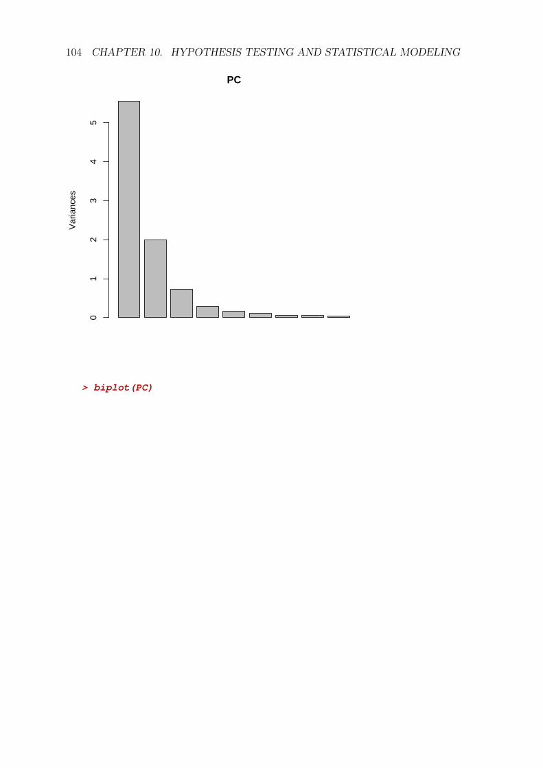
104 CHAPTER 10. HYPOTHESIS TESTING AND STATISTICAL MODELING
PCV
aria
nces
01
23
45
> biplot(PC)
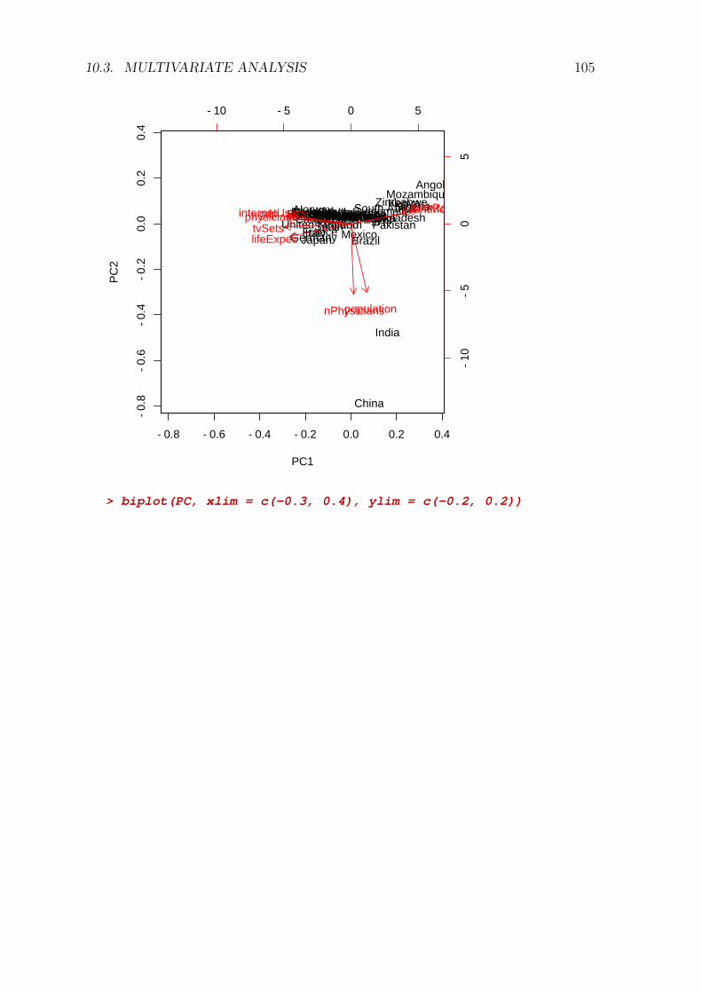
10.3. MULTIVARIATE ANALYSIS 105
−0.8 −0.6 −0.4 −0.2 0.0 0.2 0.4
−0.
8−
0.6
−0.
4−
0.2
0.0
0.2
0.4
PC1
PC
2
Albania
Angola
AustraliaAustria Bangladesh
Brazil
Canada Chile
China
Costa RicaCzech RepublicDenmark EcuadorEgyptFinland
FranceGermany
GreeceGuatemalaHungary
India
IrelandIsrael
ItalyJapan
Kenya
Mexico
Mozambique
New Zealand NigeriaNorwayPakistan
PanamaPeruPoland
PortugalSlovakiaSloveniaSouth Africa
SpainSri LankaSwedenSwitzerland
United Kingdom
Zimbabwe
−10 −5 0 5
−10
−5
05
infantMort
lifeExpec
population
birthRate
nPhysicians
physiciansgdpinternetUserstvSets
> biplot(PC, xlim = c(-0.3, 0.4), ylim = c(-0.2, 0.2))

106 CHAPTER 10. HYPOTHESIS TESTING AND STATISTICAL MODELING
−0.3 −0.2 −0.1 0.0 0.1 0.2 0.3 0.4
−0.
2−
0.1
0.0
0.1
0.2
PC1
PC
2
Albania
Angola
AustraliaAustriaBangladesh
Brazil
Canada ChileCosta RicaCzech Republic
DenmarkEcuador
Egypt
Finland
France
Germany
Greece
Guatemala
HungaryIrelandIsrael
Italy
Japan
Kenya
Mexico
Mozambique
New ZealandNigeria
Norway
Pakistan
PanamaPeru
Poland
PortugalSlovakiaSlovenia
South Africa
Spain
Sri LankaSwedenSwitzerland
United Kingdom
Zimbabwe
−10 −5 0 5 10 15
−5
05
infantMort
lifeExpec
population
birthRate
nPhysicians
physiciansgdpinternetUsers
tvSets

A Practicals
A.1 Day 1
R environment
1. Browse to http://ablejec.nib.si/R/ECPR and download I2R.ZIP to directory<HOMEDIR>/ECPR you previously made. Unzip the downloaded file in thesame directory.
2. start R and get familiar with the environment
3. change the working directory to <HOMEDIR>/ECPR/WD
4. Find help documentation for functions used in BMI analysis. Read documen-tation and try the examples
5. Browse http://www.r-project.org and CRAN. Go through the list of packagesand look for some interesting packages. Read the descriptions and documenta-tion. Look also at ’CRAN Task Views’.
R in action
1. calculate your BMI and determine your BMI code
2. Go through the material presented today, try the examples. Ask TA’s aboutanything confusing.
3. Use File | Open script to open ../doc/I2R-bmi.R Use CTRL-R to step over thelines, try to predict what line does and check the results.
107

108 APPENDIX A. PRACTICALSA.2 Day 2
1. Write a function that will add two numbers
2. Function sd returns the sample standard deviation. Write a function, that will’correct’ it to the population standard deviation (multiply by (n− 1)/n)
A.3 Readings
Browse the R web pages http://www.r-project.org
Have a look at ”R FAQs”There is a section Windows Features

B Libraries and functions
B.1 Libraries
> library(Hmisc)> library(xlsReadWrite)> library(foreign)> options(width = 80)
B.2 Functions
A collection of custom made functions is provided here.
B.2.1 catln
Concatenate and type, go to next line
> catln <- function(...) cat(..., "\n")> catln("Text1", 1234, "Text2")
Text1 1234 Text2
B.2.2 write.xls
Write data frame to Excel file. It is a write.table function, with defaults that mightbe more practical.
109

110 APPENDIX B. LIBRARIES AND FUNCTIONS
> write.xls <- function(x, file = NULL, row.names = NULL, col.names = NULL,+ sep = "\t", verbose = FALSE, ...) {+ xName <- deparse(substitute(x))+ if (is.null(file))+ file <- paste(xName, "xls", sep = ".", collapse = "")+ if (is.null(row.names))+ row.names <- !(row.names(x)[1] == "1")+ if (is.null(col.names)) {+ if (row.names)+ col.names <- NA+ else col.names = TRUE+ }+ write.table(x, file = file, row.names = row.names, col.names = col.names,+ sep = sep, ...)+ if (verbose)+ cat(xName, "written to ", file, "\n")+ }> x <- data.frame(a = letters[1:3], x = 1:3, y = sqrt(1:3))> dimnames(x)[[1]] = LETTERS[1:3]> write.xls(x, verbose = TRUE)
x written to x.xls
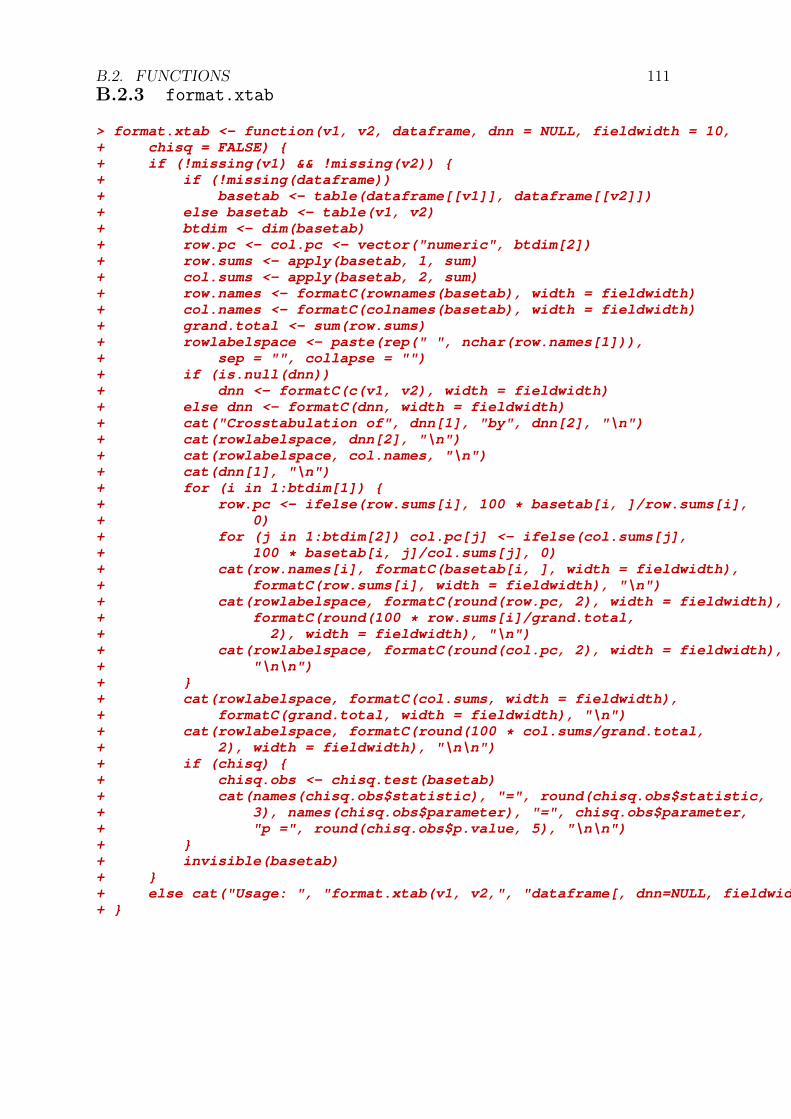
B.2. FUNCTIONS 111B.2.3 format.xtab
> format.xtab <- function(v1, v2, dataframe, dnn = NULL, fieldwidth = 10,+ chisq = FALSE) {+ if (!missing(v1) && !missing(v2)) {+ if (!missing(dataframe))+ basetab <- table(dataframe[[v1]], dataframe[[v2]])+ else basetab <- table(v1, v2)+ btdim <- dim(basetab)+ row.pc <- col.pc <- vector("numeric", btdim[2])+ row.sums <- apply(basetab, 1, sum)+ col.sums <- apply(basetab, 2, sum)+ row.names <- formatC(rownames(basetab), width = fieldwidth)+ col.names <- formatC(colnames(basetab), width = fieldwidth)+ grand.total <- sum(row.sums)+ rowlabelspace <- paste(rep(" ", nchar(row.names[1])),+ sep = "", collapse = "")+ if (is.null(dnn))+ dnn <- formatC(c(v1, v2), width = fieldwidth)+ else dnn <- formatC(dnn, width = fieldwidth)+ cat("Crosstabulation of", dnn[1], "by", dnn[2], "\n")+ cat(rowlabelspace, dnn[2], "\n")+ cat(rowlabelspace, col.names, "\n")+ cat(dnn[1], "\n")+ for (i in 1:btdim[1]) {+ row.pc <- ifelse(row.sums[i], 100 * basetab[i, ]/row.sums[i],+ 0)+ for (j in 1:btdim[2]) col.pc[j] <- ifelse(col.sums[j],+ 100 * basetab[i, j]/col.sums[j], 0)+ cat(row.names[i], formatC(basetab[i, ], width = fieldwidth),+ formatC(row.sums[i], width = fieldwidth), "\n")+ cat(rowlabelspace, formatC(round(row.pc, 2), width = fieldwidth),+ formatC(round(100 * row.sums[i]/grand.total,+ 2), width = fieldwidth), "\n")+ cat(rowlabelspace, formatC(round(col.pc, 2), width = fieldwidth),+ "\n\n")+ }+ cat(rowlabelspace, formatC(col.sums, width = fieldwidth),+ formatC(grand.total, width = fieldwidth), "\n")+ cat(rowlabelspace, formatC(round(100 * col.sums/grand.total,+ 2), width = fieldwidth), "\n\n")+ if (chisq) {+ chisq.obs <- chisq.test(basetab)+ cat(names(chisq.obs$statistic), "=", round(chisq.obs$statistic,+ 3), names(chisq.obs$parameter), "=", chisq.obs$parameter,+ "p =", round(chisq.obs$p.value, 5), "\n\n")+ }+ invisible(basetab)+ }+ else cat("Usage: ", "format.xtab(v1, v2,", "dataframe[, dnn=NULL, fieldwidth = 10, chisq = FALSE])\n")+ }
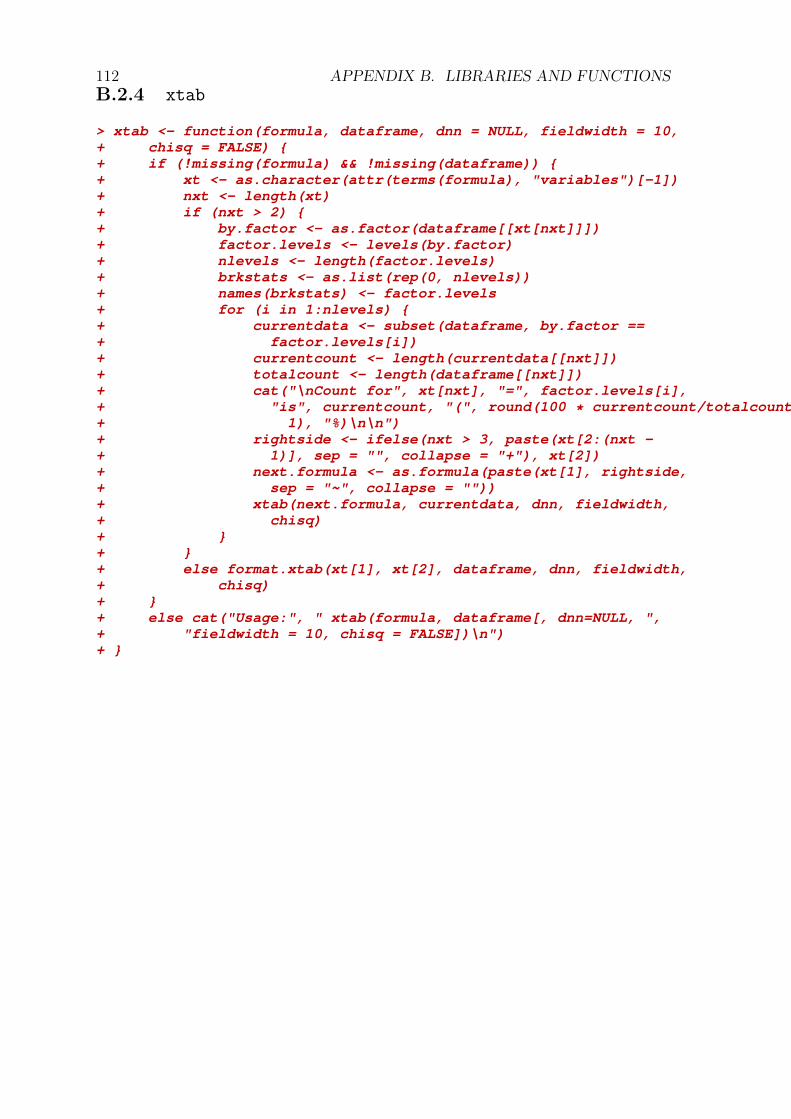
112 APPENDIX B. LIBRARIES AND FUNCTIONSB.2.4 xtab
> xtab <- function(formula, dataframe, dnn = NULL, fieldwidth = 10,+ chisq = FALSE) {+ if (!missing(formula) && !missing(dataframe)) {+ xt <- as.character(attr(terms(formula), "variables")[-1])+ nxt <- length(xt)+ if (nxt > 2) {+ by.factor <- as.factor(dataframe[[xt[nxt]]])+ factor.levels <- levels(by.factor)+ nlevels <- length(factor.levels)+ brkstats <- as.list(rep(0, nlevels))+ names(brkstats) <- factor.levels+ for (i in 1:nlevels) {+ currentdata <- subset(dataframe, by.factor ==+ factor.levels[i])+ currentcount <- length(currentdata[[nxt]])+ totalcount <- length(dataframe[[nxt]])+ cat("\nCount for", xt[nxt], "=", factor.levels[i],+ "is", currentcount, "(", round(100 * currentcount/totalcount,+ 1), "%)\n\n")+ rightside <- ifelse(nxt > 3, paste(xt[2:(nxt -+ 1)], sep = "", collapse = "+"), xt[2])+ next.formula <- as.formula(paste(xt[1], rightside,+ sep = "~", collapse = ""))+ xtab(next.formula, currentdata, dnn, fieldwidth,+ chisq)+ }+ }+ else format.xtab(xt[1], xt[2], dataframe, dnn, fieldwidth,+ chisq)+ }+ else cat("Usage:", " xtab(formula, dataframe[, dnn=NULL, ",+ "fieldwidth = 10, chisq = FALSE])\n")+ }
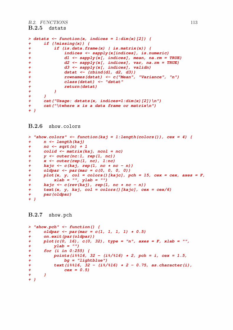
B.2. FUNCTIONS 113B.2.5 dstats
> dstats <- function(x, indices = 1:dim(x)[2]) {+ if (!missing(x)) {+ if (is.data.frame(x) | is.matrix(x)) {+ indices <- sapply(x[indices], is.numeric)+ d1 <- sapply(x[, indices], mean, na.rm = TRUE)+ d2 <- sapply(x[, indices], var, na.rm = TRUE)+ d3 <- sapply(x[, indices], validn)+ dstat <- (rbind(d1, d2, d3))+ rownames(dstat) <- c("Mean", "Variance", "n")+ class(dstat) <- "dstat"+ return(dstat)+ }+ }+ cat("Usage: dstats(x, indices=1:dim(x)[2])\n")+ cat("\twhere x is a data frame or matrix\n")+ }
B.2.6 show.colors
> "show.colors" <- function(kaj = 1:length(colors()), cex = 4) {+ n <- length(kaj)+ nc <- sqrt(n) + 1+ colid <- matrix(kaj, ncol = nc)+ y <- outer(nc:1, rep(1, nc))+ x <- outer(rep(1, nc), 1:nc)+ kajc <- c(kaj, rep(1, nc * nc - n))+ oldpar <- par(mar = c(0, 0, 0, 0))+ plot(x, y, col = colors()[kajc], pch = 15, cex = cex, axes = F,+ xlab = "", ylab = "")+ kajc <- c(rev(kaj), rep(1, nc * nc - n))+ text(x, y, kaj, col = colors()[kajc], cex = cex/6)+ par(oldpar)+ }
B.2.7 show.pch
> "show.pch" <- function() {+ oldpar <- par(mar = c(1, 1, 1, 1) * 0.5)+ on.exit(par(oldpar))+ plot(c(0, 16), c(0, 32), type = "n", axes = F, xlab = "",+ ylab = "")+ for (i in 0:255) {+ points(i%%16, 32 - (i%/%16) * 2, pch = i, cex = 1.5,+ bg = "lightblue")+ text(i%%16, 32 - (i%/%16) * 2 - 0.75, as.character(i),+ cex = 0.5)+ }+ }

114 APPENDIX B. LIBRARIES AND FUNCTIONSB.2.8 show.lty
> show.lty <- function() {+ plot(c(0, 16), c(0, 34), type = "n", axes = F, xlab = "",+ ylab = "")+ text(0.7, 33, "lwd", adj = 1)+ text(8.3, 33, "lty", adj = 0)+ for (i in 1:32) {+ segments(1, 33 - i, 8, 33 - i, col = i, lwd = i/2, lty = i)+ text(0.7, 33 - i, i/2, adj = 1, col = i)+ text(8.3, 33 - i, (i - 1)%%6 + 1, adj = 0, col = i)+ }+ text(9.7, 34, "col")+ text(15.5, 34, "cex")+ for (i in 0:16) {+ rect(10, 32 - 2 * i, 15, 32 - 2 * i + 2, col = i, border = T)+ rect(10, 32 - 2 * i, 15, 32 - 2 * i + 2, col = (i ==+ 0), density <- 0, border = T)+ text(9.7, 32 - 2 * i + 1, i)+ text(15.5, 32 - 2 * i + 1, i/5, cex = i/5)+ }+ }
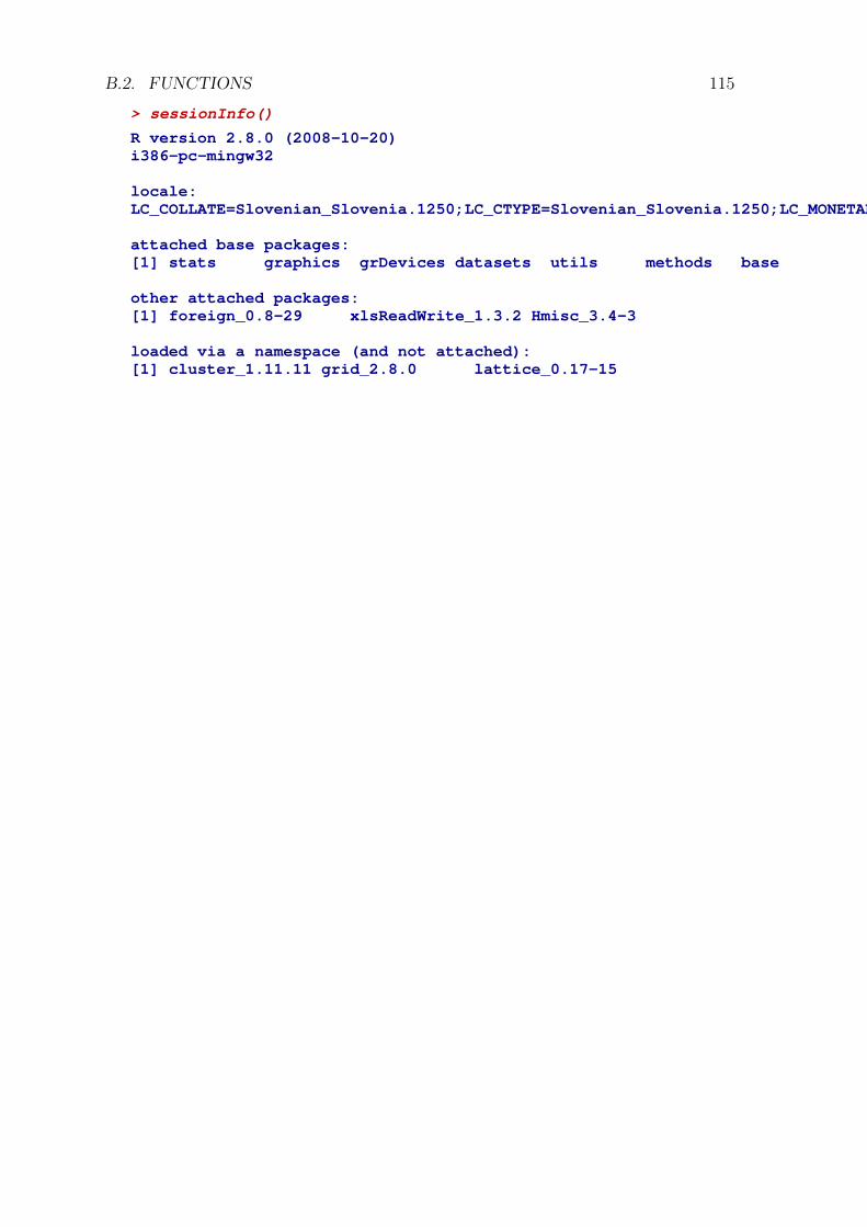
B.2. FUNCTIONS 115
> sessionInfo()
R version 2.8.0 (2008-10-20)i386-pc-mingw32
locale:LC_COLLATE=Slovenian_Slovenia.1250;LC_CTYPE=Slovenian_Slovenia.1250;LC_MONETARY=Slovenian_Slovenia.1250;LC_NUMERIC=C;LC_TIME=Slovenian_Slovenia.1250
attached base packages:[1] stats graphics grDevices datasets utils methods base
other attached packages:[1] foreign_0.8-29 xlsReadWrite_1.3.2 Hmisc_3.4-3
loaded via a namespace (and not attached):[1] cluster_1.11.11 grid_2.8.0 lattice_0.17-15

116 APPENDIX B. LIBRARIES AND FUNCTIONS

C Data
C.1 Data sources
C.1.1 Statistical Yearbook of RS, Statistical Office of RS
http://www.stat.si/letopis/index_vsebina.asp?poglavje=14&leto=2006&jezik=si
C.1.2 NationMaster
http://www.nationmaster.com/statistics
C.1.3 Technology, Entertainment, Design (TED)
Hans Rosling lecturehttp://www.ted.com/tedtalks/tedtalksplayer.cfm?key=hans_rosling
117
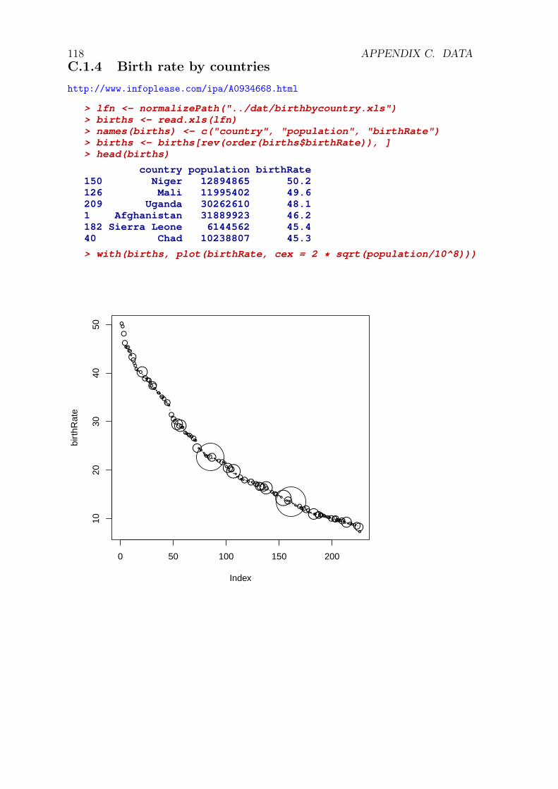
118 APPENDIX C. DATAC.1.4 Birth rate by countries
http://www.infoplease.com/ipa/A0934668.html
> lfn <- normalizePath("../dat/birthbycountry.xls")> births <- read.xls(lfn)> names(births) <- c("country", "population", "birthRate")> births <- births[rev(order(births$birthRate)), ]> head(births)
country population birthRate150 Niger 12894865 50.2126 Mali 11995402 49.6209 Uganda 30262610 48.11 Afghanistan 31889923 46.2182 Sierra Leone 6144562 45.440 Chad 10238807 45.3
> with(births, plot(birthRate, cex = 2 * sqrt(population/10^8)))
●●
●
●●●●
●●●
●●●●●●
● ●
●●●
●●●●
●●●●●●●●
●
●●●
●●●●●
●●●●
●
●●
●●
●●●●●●●●●
●●●●●●●●
●●●
●● ●●
●●
●
●
●●●●●●● ● ●●
● ●●●
●●● ● ●
●●●●●●●● ●
●
● ● ●●●●●●●
●●●●●●●● ●●●●●●●●●●●●● ●
●
●●●●●●● ●
●●
●●●
●
●●●●●
●
● ●
●● ● ●●●●●●●●●●
●●
●●●●●●●●●●●●●●●●●●●●●
●●●●●●●●●●●●●●
● ●●●●●●●●●●●
0 50 100 150 200
1020
3040
50
Index
birt
hRat
e

C.2. DATA SETS 119C.2 Data sets
C.2.1 Infant Mortality and Life Expectancy, 2007
http://www.infoplease.com/ipa/A0004393.html
> lfn <- normalizePath("../dat/mortality.xls")> mortality <- read.xls(lfn)> names(mortality)
[1] "continent" "country" "infantMort" "lifeExpec"
> head(mortality)
continent country infantMort lifeExpec1 Europe Albania 20.0 77.62 Africa Angola 184.4 37.63 Pacific Australia 4.6 80.64 Europe Austria 4.5 79.25 Asia Bangladesh 59.1 62.86 S America Brazil 27.6 72.2
> with(mortality, plot(infantMort, lifeExpec))
●
●
●●
●
●
●
●
●
●●
●
●●
●
●●●●
●
●
●
●
●
●●
●
●
●
●
●
●
●
●
●
●
●
●
●
●
●
●
●
●
●●
●
●●
●
●
●
0 50 100 150
4050
6070
80
infantMort
lifeE
xpec

120 APPENDIX C. DATAC.2.2 Number of Physicians and Physicians per 1000 inhab-
itants
http://www.who.int/whosis/en/
> lfn <- normalizePath("../dat/physicians.xls")> physicians <- read.xls(lfn)> head(physicians)
country nPhysicians physicians1 Afghanistan 4104 0.192 Albania 4100 1.313 Algeria 35368 1.134 Andorra 244 3.705 Angola 1165 0.086 Antigua and Barbuda 12 0.17
> with(physicians, {+ select <- (country == "Slovenia") + 1+ col = c(1, 2)[select]+ pch = c(1, 16)[select]+ plot(nPhysicians, physicians, col = col, pch = pch, cex = select,+ log = "xy")+ })
●
●●
●
●
●
●●
●
●●
● ●
●
●
●●
●
●
●
●●
●
●●
●
●
●
●●
●
●
●
●
● ●
●
●
●
●
●
●
●
●
●
● ●
●
●
●
●
●
●
●
●
●
●
●
●
●
● ●
●
●
●
●
●
●
●
●
●●
●
●
●
●●
●
●
●
●
●
●●
●
●●
●
●
●
●
●●
●
●
●
●
●
●
●
●
●
●
●
●
●
●
●
●
●
●
●
●
●●
●
●
●
●
●
●
●
●
●
●
●
●
● ●
●
●
●
●
●
●
●
●
●
●
●
●
●
●
●
●
●
●
●
●
●
●
●
●
●
●
●
●
●
●●
●
●
●
●●
●
●
●
●
● ●
●
●
●
●
●●
●
●
●
●
●
●
●
●
●
●
1e+01 1e+03 1e+05
0.02
0.05
0.10
0.20
0.50
1.00
2.00
5.00
nPhysicians
phys
icia
ns
Both axes are logarithmic. Red dot represents Slovenia.

C.2. DATA SETS 121C.2.3 GDP per capita (USD), 2005
http://www.who.int/whosis/en/
> lfn <- normalizePath("../dat/gdp2005.xls")> gdp2005 <- read.xls(lfn)> head(gdp2005)
country gdp1 Albania 54202 Algeria 67703 Angola 22104 Antigua and Barbuda 117005 Argentina 139206 Armenia 5060
> with(gdp2005, barplot(gdp[order(gdp)], hori = TRUE, main = "GDP 2005"))> cName <- "Slovenia"> slo <- gdp2005[gdp2005$country == cName, ][2]> abline(v = slo, col = 2)> text(slo, par("usr")[4] * 1.05, cName, xpd = TRUE, col = "red")
GDP 2005
0 10000 20000 30000 40000 50000 60000
Slovenia

122 APPENDIX C. DATAC.2.4 Internet users (per 1000), 2002
http://www.who.int/whosis/en/
> lfn <- normalizePath("../dat/internet2002.xls")> internet2002 <- read.xls(lfn)> head(internet2002)
country internetUsers1 Albania 42 Algeria 163 Angola 34 Antigua and Barbuda 1285 Argentina 1126 Armenia 16
> with(internet2002, plot(internetUsers))
●●●
●●
●
●
●
●
●
●
●
●
●
●
●
●●●●●
●●●
●●●●
●
●
●●
●
●●
●●
●
●
●
●
●
●
●
●
●
●●●●
●●
●
●
●
●
●
●●●
●
●
●●
●
●●
●
●●
●
●
●●
●
●
●●
●
●
●
●
●●●
●
●
●
●●
●●
●
●
●
●●
●
●
●
●
●●
●●
●
●●●●
●●
●
●
●
●●●
●
●
●
●
●●
●
●
●
●
●
●
●
●
●
●
●
●
●
●
●
●●
●
●
●
●
●
●
●●
●
●
●●
●
●
●
●
●●
●●●●●
●
●●
●
●
●●
●
●
●
●
●
●
●●
●●●
●
0 50 100 150
010
020
030
040
050
060
0
Index
inte
rnet
Use
rs

C.2. DATA SETS 123C.2.5 Number of TV sets per 1000
http://www.nationmaster.com/red/graph/med_tel_percap-media-televisions-per-capita&b_
desc=1
> lfn <- normalizePath("../dat/tv.xls")> tv <- read.xls(lfn)> names(tv)[2] <- "tvSets"> head(tv)
country tvSets1 Afghanistan 3.34002 Albania 196.46403 Algeria 95.29084 American Samoa 241.87605 Andorra 382.71306 Angola 16.5723
> with(tv, plot(tvSets))
●
●
●
●
●
●
●
●
●
●●
●●
●
●
●
●
●●
●
●
●
●
●
●
●
●●
●
●
●●●●●
●
●
●
●●
●
●
●
●
●●
●
●
●
●
●
●●●
●
●●
●●
●
●
●
●
●
●
●●
●
●
●
●
●
●
●
●
●
●
●
●
●
●
●
●
●
●
●
●●●●
●
●
●
●
●
●
●
●●
●
●
●
●●
●
●
●
●
●
●
●
●
●
●
●
●●
●
●
●
●
●
●
●
●
●
●
●
●
●
●●●
●
●
●
●
●
●
●
●
●
●
●
●
●
●
●
●
●
●●
●●
●
●
●
●●
●
●
●
●
●
●
●
●
●
●
●
●
●
●
●●
●
●
●●
●
●
●
●
●
●
●
●
●
●●
●
●
●
●
●
●
●
●
●
●
●●
●
●
●
●
●●●
0 50 100 150 200
020
040
060
080
010
00
Index
tvS
ets

124 APPENDIX C. DATAC.3 Merged data set
The data are merged into one dataset, based on the country names.
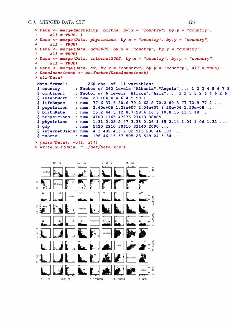
C.3. MERGED DATA SET 125
> Data <- merge(mortality, births, by.x = "country", by.y = "country",+ all = TRUE, )> Data <- merge(Data, physicians, by.x = "country", by.y = "country",+ all = TRUE)> Data <- merge(Data, gdp2005, by.x = "country", by.y = "country",+ all = TRUE)> Data <- merge(Data, internet2002, by.x = "country", by.y = "country",+ all = TRUE)> Data <- merge(Data, tv, by.x = "country", by.y = "country", all = TRUE)> Data$continent <- as.factor(Data$continent)> str(Data)
'data.frame': 260 obs. of 11 variables:$ country : Factor w/ 260 levels "Albania","Angola",..: 1 2 3 4 5 6 7 8 9 10 ...$ continent : Factor w/ 6 levels "Africa","Asia",..: 3 1 5 3 2 6 4 6 2 6 ...$ infantMort : num 20 184.4 4.6 4.5 59.1 ...$ lifeExpec : num 77.6 37.6 80.6 79.2 62.8 72.2 80.3 77 72.9 77.2 ...$ population : num 3.60e+06 1.23e+07 2.04e+07 8.20e+06 1.50e+08 ...$ birthRate : num 15.2 44.5 12 8.7 29.4 16.3 10.8 15 13.5 18 ...$ nPhysicians : num 4100 1165 47875 27413 38485 ...$ physicians : num 1.31 0.08 2.47 3.38 0.26 1.15 2.14 1.09 1.06 1.32 ...$ gdp : num 5420 2210 30610 33140 2090 ...$ internetUsers: num 4 3 482 415 2 82 513 238 46 193 ...$ tvSets : num 196.46 16.57 505.23 519.24 5.34 ...
> pairs(Data[, -c(1, 2)])> write.xls(Data, "../dat/Data.xls")
infantMort
40 70
●
●
●●
●●
●●●●●●●●●●●●●
●●
●●●●●●
●
●●
●
●
●
●
●
●●●●● ●●
●
●●●●
●●●
●●
●
●
●●
●●
●●●●●●●
●●●●●●●●
●●●●●●
●
●●
●
●
●
●
●
●●●●●●●
●
●●●●●● ●●●
10 40
●
●
●●
●●
●●●●●●●●●
●●●●●
●●●
●●●●
●
● ●
●
●
●
●
●
●●●●●●●
●
●●●●
●●●●
●●
●
●●
●●
●●●●●●●
●●●●●●●●
●●●●●
●●
●
●
●
●
●
●●●●●●
●
●●●●●
●
0 3 6
●
●
●●
●●
●●●● ● ●●●●
●●● ●●
●●
● ●●●
●●
●
●
●
●
●
●● ●●●●
●
●●●●●
●●
●
●●
●●
●●●● ●● ●●●
●●●●●
●●●
●●●●
●●
●
●
●
●
●
●●●●●●
●
●●●●●
●●
0 400
●
●
●●
●●
●●● ●●● ●●●
●● ●●●
●●●
●●●●
●●
●
●
●
●
●
●●●●● ●
●
●●●●●
●●
015
0
●
●
●●
●●
●●●● ● ●●●
●●●●●
●●●
●● ●●
●●
●
●
●
●
●
●● ●●●●●
●
●●●●
●● ●●
●
4070
●
●
●●
●
●●●●
●●●●●●
●●●●
●●●●
●●●●
●
●●
●
●
●
●
●
●●
●●
●●●
●
●●
●●
●●●●
●
lifeExpec
●
●
●●
●
●●●
●●●●●●●
●●●●
●● ●●●●●●
●
●●
●
●
●
●
●
●●●●
●●●
●
●●●●
●● ●●
●
●
●
●●
●
●●●●
●●●● ●●
●●●●
●●●●
●●●●
●
● ●
●
●
●
●
●
●●
●●
●●●
●
●●
●●
●●●●
●
●
●
●●
●
●●●
●●●●●●●●●●●
●● ●●●●●
●
●
●
●
●
●
●
●●●●●●
●
●●●●●
●
●
●
●●
●
●●●
●● ● ●●●
●●●● ●
● ●●
● ●●●
●
●
●
●
●
●
●
●●
●●●●
●
●●
●●●
●
●
●
●●
●
●●●
●● ●● ●●
●●●●●
● ●●●
●●●●
●
●
●
●
●
●
●
●●
●●●●
●
●●
●●●●
●
●
●
●●
●
●●●
●●●● ●●
●●● ●●
● ●●●
●●●●
●
●
●
●
●
●
●
●●
●●● ●
●
●●
●●●●
●
●
●
●●
●
●●●
●● ● ●●●
●●●●
● ●●●
●● ●●
●
●
●
●
●
●
●
●●
●●
●●●
●
●●
●●
●● ●●
●
● ●●●●●
●●
●
●●●●●●●●●●●●
●
●●●●● ●●● ●●
●●
●●●●●●●● ●●●●●●●●● ● ●● ●●
● ●●●
●
●●●●●●●●●●●●
●
● ●●●●● ●●● ●
●●
●●●●●
●●●● ●●●●● ●●
●●
population
● ●●●●●
●●
●
●●●● ●●●●●● ●●
●
●●●●● ●● ● ●●●
●●
●●●●●●● ●●●●● ●●●
● ● ●●●●●●●●●●●●●●● ● ●● ●●● ●●● ●● ●● ●●● ● ●● ●●● ●●● ●● ●●● ●●● ●● ●●● ●●●● ●●●●●●● ●●● ●●●●●
●● ●● ●● ●●●● ●● ●● ●●●●●●● ●● ● ●● ●● ●● ●●●● ●●●●●●●●●●● ●● ●● ●●●●●●● ●●●●●●●● ●● ●●● ●● ● ●●● ●● ● ●● ●●●●● ●●● ●● ●● ●●●●●● ● ●●● ●●●●●●●●
●
●●●●●●●●●●●●
●
●●●●●●●●●●●
●●●●●●●●●●●●●●●●●●●●●●●●●●●●●●●●●●●●●●●●●●●●●●●●●●●●●●●●●●●●●●●●●●●●●●●●●●●●●●●●●●●●●●●●●●●●●●●●●●●●●●●●●●●●●●●●●●●●●●●●●●●●●●●●●●●● ●● ●●
●●●●
●
● ● ●●●● ●●● ●● ●
●
● ●●●● ●● ●
●●
●●● ●●●●● ●● ●●●●●● ●● ●●●●● ●●●●● ●●● ●●●●●●●● ●●●● ● ●●● ●●●● ●●●● ●●●●●●●● ●
●●● ● ●● ● ●●●●● ●●●●●● ●●●● ●●●● ●●● ●●● ●● ●●● ● ●●●●●● ●● ●●●●●● ●●●●●●● ●●● ●● ●●●●● ●● ●●
●●●●
●
● ●● ●●● ●●●●● ●
●
● ●●●●●●● ●
●●
●●●●●●●● ●● ●●●●●●●●●● ●● ●●●●●●●●●●●●●●●●● ●●●●●●● ●●●●●●●●●●●● ●
●●●● ●● ●●● ● ●●●●● ●●●●●●● ●●● ●●●●●● ●●●●●● ●● ●●●●●●●●●●●●●● ●●●●●● ●● ●●
●●●●
●
●●● ●●● ●● ●●● ●
●
● ●●●●●●● ●●
●●●● ●●● ●● ●● ●●●●●● ●●●● ●●● ●●●●●●●●●●●●●●●●●● ●●● ●●●●● ●●●●●● ●●● ●●● ●●● ●●●●●●●●●● ● ●●● ●●● ●●●●●●●●●●● ●●●●●●●●●● ●●●● ●●●● ●● ●●●●●●●●●●●●●● ●●● ●●●●●●
0.0e
+00
●● ●●● ●
●●
●
● ● ●●● ●●●●● ●
●
● ●● ●●● ●● ●●
●●
●● ●●●●●● ●● ●●● ●
●●●●●●●● ●●●●● ●●● ●●● ●●●● ●●●●●●●●●●●●●●● ●●●●●●●● ●● ●●●●● ●● ● ●●● ●●●●● ●●
●●●● ●● ●●● ●●●● ●●●● ●●● ●●● ●●● ● ●● ●●●●● ●●●●● ●●●●● ●●●●●●● ●●● ●●●●●● ●●●●●● ●●● ●●● ●● ●●●● ●●●●●● ●●●
1040
●
●
●●
●
●●●●●●●●
●●
●●●●
●
●
●●●●
●●
●
●
●
●
●
●
●
●●●
●●●●●●
●●
●●
●
●●●
●
●
●
●●
●
●●
●●●●●●
●●
●●●●
●
●
●● ●●
●●
●
●
●
●
●
●
●
●●●
●●● ●●●
●●
●●
●
●●●
●
●
●
●●
●
●●● ●●●●●
●●
●●●●
●
●
●●●●
●●
●
●
●
●
●
●
●
●●●
●●●●●●●●●●
●
● ●●
●
●
●●
●●●●●●●●●●●●
●
●
●
●
●
●
●●●
●
●
●
●●
●
●
●
●
●
●●
●
●
●●
●
●●●●●●
●
●
●●●●
●●●
●
●
●●●●●
●
●●
●
●●
●●
●
●
●
●
●
●●
●
●●●
●
●●●
●
●
●●●●●
●
●
●
●
●
●
●
●
●
●
●
●●
●
●●●●●●
●●●●
●
●
●
●
●●●
●●●●
●
●●●●●●●
●
●●
●●
●
●
●
●
●
●
●
●
●
●
●
●
●
●●●
●●●
●
●
●●
●●●●●
●
●
●●●
birthRate●
●
●●
●
●●● ●●●●●
●●
●●●●
●
●
●●●
●●
●
●
●
●
●
●
●●●
●●●●●●
●●●●
●
●
●●●●●●●●●●
●
●●
●
●
●
●
●●
●●
●●
●
●
●●
●
●●
●
●●●●●
●
●
●
●
●
●●
●●
●
●●
●●
●
●●●
●●●
●●●
●
●●
●
●
●
●
●
●●
●●●●●
●
●
●
●
●
●●●●●
●
●●●●
●
●●
●
●
●
●
●
●
●
●●
●
●
●
●●●
●●
●
●
●●
●●
●●
●
●
●●
●
●●
●●●
● ●●
●●
●●● ●
●
●
●● ●
●●
●
●
●
●
●
●
●●●
●●●●●
●●
●●●
●
●
●●
● ●●●●
● ●●
●
●●
●
●
●
●
●●
●●
●●
●
●
●●
●
● ●
●
●●●
●●
●
●
●
●
●
●●
●●
●
●●
●●
●
● ●●
●● ●
●●
●
●
●●
●
●
●
●
●
●●
●●●●
●
●
●
●
●
●
● ●●
●●
●
● ●●●
●
●●
●
●
●
●
●
●
●
● ●
●
●
●
●●●
●●
●
●
●●
●●
●●
●
●
●●
●
●●
●●●
●● ●
●●
●●●●
●
●
●● ●●
●●
●
●
●
●
●
●
●●●
●●●●●
●●
●●●●
●
●●●●● ●● ●
●
●
●
●
●
●
●●
●●
●●
●
●
●●
●
●
●●●●●
●
●
●
●
●
●●
●●
●
●●
●●●●●
●●
●●●
● ●●
●
●
●
●
●
●●●●●
●
●
●
●●●●
●
●
●●●●
●●
●
●
●
●●●●
●
●
●
●
●●●
●
●
●●
●●
●●
●
●
●●
●
●●
●●●
●● ●
●●
●●●●
●
●
●● ●●
●●
●
●
●
●
●
●
●●●
●●● ●●
●●
●●●●
●
● ●●●● ●
●● ●
●
●●
●
●
●
●
●●
●●
●●
●
●
●●
●●
●
●●●
●●
●
●
●
●
●
●●
●●
●
●●
●●
●
●●●
●●●
●●
●
●
● ●●
●
●
●
●
●
●●
●●
●
●●●●●
●
●
●
●●●●
●●
●
●●●●●
●
●●
●
●
●
●
●
●
●
●●
●
●
●
●●●
●●
●
●
●●
●●
●●
●
●
●●
●
●●
●●●
● ●
●●
●●●●
●
●
●● ●●
●●
●
●
●
●
●
●
●●●
●●●●●●
●●
●●
●
● ●●
●
●
●●
●● ●●
●●● ●
●● ●
●
●
●
●
●●●
●
●
●
●
●●
●
●
●
●
●
●●●
●●
●
●●●
●●
●
●
●●●●
●
●
●
●●
●●
●
●
●
●●
●●
●
●
●●●
●●●
●
●●
●
●
●●●
●
●
●
●
●●
●
●
●
●
● ●
●●
●●●●
●●●
●
●
●
●
●●●
●●●●●●●
●●●●
●
●●
●
●
●
●
●
●
●
●
●
●
●
●
●
●
●● ●
●●
●
●
●●
●●● ●
●●
● ●●● ●●
●●
●
●●●●●●●●●●●●
●
●●●●
●●
●● ●● ●●●●●●● ●●●●●● ● ●● ●●●
●●●
●
●●●●●●●●●●●●
●
●●●●
●●
● ●● ●● ●●●●●●● ●●●●●● ●●●●●
●●●
●
●●●●●●●●●●●●
●
●●●●●●
●●●●●●●●●●●●●●●●●●●●●●●●●●●●●●●●●●●●●●●●●●●●●●●●●●●●●●●●●●●●●●●●●●●● ●●●●●●●●●●●●●●●●●●●●●●●●●●●●●●●●●●●●●●●●●●●●●●●●●●●●●●●●●●●●●●●●●●●●● ● ●●● ●
●●●
●
●●●● ●●●●●
● ●●
●
●●●●
●●
●● ●● ●●●●●●● ●●●●●● ● ●●● ●●●●●●●● ● ●●●● ●● ●●● ●● ● ●● ●●●●● ●● ●● ●●● ●● ●● ●● ●●● ●●●● ●●●● ●●●● ●● ●●● ●● ● ●● ● ●●●●●●● ● ●●● ●●●●● ●●●●● ●● ●● ●● ● ●●● ●●● ●●●●● ●● ●
●●● ●● ●●
nPhysicians
●● ●●●●
●●
●
● ● ●●●● ●●●
●● ●
●
● ●●●
●●
● ●● ●●●● ●●●●● ●● ●●●
●●● ●● ●●●●● ●●●●● ●●● ●●●●●●●● ●●●● ● ●●● ●●●● ●●●● ●●●●●●●● ●●●● ● ●● ● ●●●●● ●●●●●● ●●●● ●●●● ●●● ●●● ●● ●●● ● ●●●●●● ●● ●●●●●● ●●●●●●● ●●●●
● ●●●●●●●● ●●●●●●●● ● ●
●
●●●●●
●
●● ●● ●●●●
●●
●
● ●● ●●● ●●●
●● ●
●
●●●●
●●
● ●● ●●●●●●●●● ●● ●●●●●●●●● ●● ●●●●●●●●●●●●●●●●● ●●●●●●● ●●●●●●●●●●●● ●●●●● ●● ●●● ● ●●●● ●●●●●●● ●●● ●●●●●● ●●●●●● ●● ●●●●●●●●●●●●●
●●●●●●●●● ●●
●
●● ●● ●●●●
●●
●
●●● ●●● ●● ●
●● ●
●
●●●●
●●
● ●● ●●●● ●●● ●● ●● ●●●●● ●●●● ●●● ●●●●●●●●●●●●●●●●●● ●●● ●●●●● ●●●●●● ●●● ●●● ●●● ●●●●●●●●●● ● ●● ●●● ●●●●●●●● ●●●●●●●●●● ●●●●●●● ●● ●●●●●●●●●●●●●● ●●●
●●●●●● ●●●●●●●
●
●●
●
● 012
0000
0
●● ●●●●
●●
●
● ● ●●● ●●●
●● ●
●
●●●●
●●
● ●● ●●●● ●● ●●● ●● ●●●●●● ●●●●● ●●● ●●●●●● ●●●●●●●●●●●●●●●●●●● ●●●● ●● ●●●●● ●●●●● ●● ●● ●●● ●●● ●●● ●● ●●●●● ●●● ●●●●● ●●●●●●●●●●● ●●●●●●●●●● ●● ●●●●
●●●●●●● ●
03
6
●●
●●
●●
●●●●●●●
●●
●●●●
●
●
●
●●●
●
●
●
●
●
●
●
●●●
●●●●
●
●
●
●●
●
●●
●
●●
●●
●●●●●●●
●●
●●●●
●
●
●
●●●
●
●
●
●
●
●
●
●●●
●●●●
●
●
●
●●
●
●●●
●●
●●
●● ●●●●●
●●
●●●●
●
●
●
●●●
●
●
●
●
●
●
●
●●●
●●●●
●
●
●
●●
●
●●●
●
●
●●●
●●
●●
●●●●●●
●
●●●●●●●
●●●●
●
●
●●
●●●●
●
●●●
●
●●●●●●●
●
●●●●
●
●●●●●
●●
●
●
●●●●
●
●●●
●
●●●
●
●●
●●●●●
●●
●●
●
●●●●
●
●
●
●
●●●●●
●
●●●●●●
●
●●
●●
●●
●●●●
●
●●
●●
●●●●
●●●
●●
●●●●
●
●
●
●●●
●
●
●
●
●
●
●
●●●
●●●●
●
●
●
●●
●
● ●●
●
●
●●●
●●
●●
●●●
●●●
●
●●● ●● ● ●
●●●
●
●
●
●●
●●
●●
●
●● ●
●
●● ●●● ●●
●
●●●
●
●
●●●● ●
● ●
●
●
●● ●●
●
● ●●
●
●●●
●
● ●
●●●●
●
●●
●●
●
●● ●●
●
●
●
●
● ●●● ●
●
● ●●●●●
●
● ●
●●
●●
● ●●●●
●●
●●
●● ●●●●●
●●
●●●●
●
●
●
●●●
●
●
●
●
●
●
●
●●●
●●●●
●
●
●
●●
●
●●●
●
●
●●●
●●
●●
●●●●●●
●
●●●●●●●
●●●●
●
●
●●
●●●●
●
●●●
●
●●●●●●●
●
●●●●
●
●●●●●
●●
●
●
●●●●
●
●●●
●
●●●
●
●●
●●●●●
●●
●●
●
●●●●
●
●
●
●
●●●●●
●
●●●●●●
●
●●
●●
●●
●●●●●●
●
●●●●
●●●●●
●
●●●
●●
●●
●
physicians●
●
●●
●●
●●●●
●●
●
●●
●●●●
●
●
●
●●●
●
●
●
●
●
●
●
●●●
●●●●
●
●
●
●●
●
●●●
●●●
●
● ●
●●●●
●
●
●●●●●●●
●●●
●
●●
●●●●
●
●●●
●
●●●●●●●
●
●●●
●
●● ●●
●
●
●
●●●
●
●●
●
●●●
●
●●
●
●●●
●
●●
●
●●●
●
●
●
●
●●●
●
●●●●●●
●
●●
●●
●●●●●●
●●
●
●●
●●
●●
●●
●●● ●●
●●
●●
●● ●●
●
●
●
●●●
●
●
●
●
●
●
●
●●●
●●●
●
●
●
●
●●
●
●●
●
●●●
●●
● ●
●●●●●●
●
●●●●●●●
●●●
●
●
● ●
●●
●●
●
●●●
●
● ●●● ●●●
●
●● ●●
●
●●
●●●
●●
●
●
● ●●●
●
●●●
●
●●●
●
●●
●
●●●
●●
●●
●
●●●●
●
●
●
●
●●●●●
●
●●●●
●●
●
●●
●●
●●
●●●●●
●●●
●●
●
●
●
●
●●
●
●●
●●
●●●●
●●
●●
●●●●
●
●
●
●● ●
●
●
●
●
●
●
●
●●●
●● ●●
●
●
●
●●
●
●●●
●
●
●●●
●●
● ●
●●●●
●
●
●●●●●●●
●●●
●
●
●●
●●
●●
●
●●●
●
● ●●●●●
●
●●●●
●
●●
● ●●
●
●
●
● ●●●
●
●●
●
●●●
●
●●
●●●
●●
●●●
●
●●●●
●
●
●
●
●●●●●
●
●●●●
● ●
●
●●
●●
●●
●●●●
● ●
●●
●●
●
●●●●●●
●●
●●●●
●●
●●
●●●●
●●
●
●
●
●
●●●●●●●
●●
●
●●●
● ● ●●
●●
●●
●
●●●●●●
●●
●●●●
●●
●●
●●●●
●●
●
●
●
●
● ●●●●●●
●●
●
●●●
●● ●●
●●
●●
●
● ●●●●●
●●
●●●●
●●
●●
●●●●
●●
●
●
●
●
●●●●●●●●●
●
●●●
●●●●●●●
●●
●
●●●●●●●●●●●●●●●●●●●●●●●
●
●●●●●●●●●●●
●
●●●●
●
●●●●●
●
●●●●
●
●●●●●●
●
●●
●●●●●●●●●●●●
●
●
●
●●●●●●●●●●●●●
●
●●●●● ● ●
●●
●●
●
●●●●●●
●●
●●●●
●●
●●
●●●●
●●
●
●
●
●
●●●●●●●
●●
●
●●●
● ●●●●
●●
●●
●
●●●● ●●
●●● ●● ● ●● ●●
●●● ●● ●
●
●
●● ●● ●● ●●● ●●
●
●●●●
●
●●
●●●
●
●●
●●
●
●●
●●●
●
●
● ●
●●●●●
●●●●●
●●
●
●
●
●●●● ●●
●●●●●
●●
●
●●● ●● ●●
●●
●●
●
● ●●●●●
●●
●●●●
●●
●
●●●●
●●
●
●
●
●
●●●●●●●●●
●
●●●
●●●●●●
●●
●
●●●●●●●●●●●●●●●●●●●●●●●
●
●●●●●●●●●●●
●
●●●●
●
●●●●●
●
●●●
●
●●●●●●
●
●●
●●●●●●●●●●●●
●
●
●
●●●●●●●●●●●●
●
●●●●●●●●
●
●●
●● ●●
●●
●●
●
●●●● ●
●
●●
●●●●
●●
●
●●●
●
●●
●
●
●
●
●●●●
●●●
●●
●
●●●
●●● ●●●
●●
●
●● ●●● ●
●●●●●●●●●●
●●● ●●●●
●
●●● ●●●●●●●●
●
●● ● ●
●
●●●●
●
●
●●
●
●
●●
●●●●
●
●●
●● ●● ●●
●●●●
●●
●
●
●
●●● ●●
●●●●●● ●
●
●●●●●●●●
●
●●
●●
gdp
●●
●●
●●
●
●● ●●●
●
●●
●● ●●
●●
●●
●●●●
●●
●
●
●
●
●●●●
●●●
●●
●
●●●
●●●●●
●●
●●
●
●●●●●●●●●●●●●●●●
●● ●●●●●
●
●●●●● ●●● ●●●
●
● ●●●
●
●●●●●
●
●●
●●
●
●●
●●●●
●
●●
●●●●
●●
●●●●●
●
●
●
●
●●●●●
●●●●●●●
●
●●●●●●●●●●● 0
5000
0
●●
●●
●●
●
●●●●
●
●●
●●●●
●●
●●
●● ●●
●●
●
●
●
●
●●●●● ●●
●●
●
●●●
●●●●●
●●
●●
●
●●●● ●●●●●●●●●●●
●●●●●●
●
●
●●● ●● ●●●●●
●
●●● ●
●
●●
●●
●
●●
●
●
●●
●●●●
●
●●
●●●● ●●●●●
●●
●
●
●
●●●●●●
●● ●● ●● ●
●
●●●●●
040
0
● ●
●●
●●
●
●
●
●●●
●
●●
●
●●
●●
●
●●
●●●●
●●
●
●
●
●
●●●
●●●
●
●●
●
●
●●
● ● ●●
●●
●●
●
●
●
●●●
●
●●
●
●●
●●●
●●
●●●●
●●
●
●
●
●
● ●●
●●●
●
●●
●
●
●●
●● ●●
●●
●●
●
●
●
●●●
●
●●
●
●●
●●●
●●
●●●●
●●
●
●
●
●
●●●
●●●
●
●●
●
●
●●
●●●●●●●
●●●
●
●●●●●●●●●●●●●●●●●
●
●●
●●●●●
●
●●●●●●●●●●●
●
●●
●
●●●●●●●●●
●
●
●●
●
●●
●
●●●●●●●●●●
●
●●●●●●●●●
●●●●
●
●●●●
●
●
●●●●●●●●●●●●●●●●
●
●●●●● ● ●
●●
●●
●
●
●
●●●
●
●●
●
●●
●●
●
●●
●●●●
●●
●
●
●
●
●●●
●●●
●
●●
●
●
●●
● ●●●●
●●
●●●
●
●●●●● ●●
●●● ●● ● ●● ●●
●
● ●
●●● ●●
●
●● ●● ●●
●●●
●●
●
● ●
●
●● ●●●
● ●● ●
●
●
● ●
●
● ●
●
● ●● ●● ●●●●●
●
● ●●
●●●●●
●
●●●●
●
●● ●●
●
●
● ●●● ●●● ●●●●● ●
●●●
●
●●● ●● ●●
●●
●●
●
●
●
●●●
●
●●
●
●●
●●●
●
●●●●
●●
●
●
●
●
●●●
●●●
●
●●
●
●
●●
●●●●●●
●●●
●
●●●●●●●●●●●●●●●●●
●
●●
●●●●●
●
●●●●●●●●●●●
●
●●
●
●●●●●●●●●
●
●
●
●
●●
●
●●●●●●●
●
●●●●●●●●●
●●●●●●●●
●
●
●●●●●●●●●●●●●●●●
●
●●●●●
●●●●●●● ●●●
●
● ●●
●●
●●
●
●
●
●● ●
●
●●
●
●●
●●
●
●
● ●●●
●●
●
●
●
●
●●●
●●●
●
●●
●
●
●●
●●● ●
●●
●● ●
●
●●● ●●● ●●●●●●●● ●●●
●
●●
●●●●●
●
●●● ●●●
●●●●●
●
●●
●
● ●●●
●●●
●●
●
●
●
●
●●
●
●●●
●●●●
●
●●●
● ●●●●
●
●●●●●●●
●
●
●
●●●●● ●●●●●●● ●●
● ●
●
●●●●●
●●
●● ●●● ●●●
●
● ●●
●●
●●
●
●
●
●●●
●
●●
●
●●
●●
●
●●
●●●●
●●
●
●
●
●
●●●
●●●
●
●●
●
●
●●
●●●●●
●●
●
●
●
●●●●●●●●●●●●●●●●
●
●
●●●●●
●
●●●●●●
●●●●●
●
●
●
●●●
●●●
●●
●
●●
●
●
●
●●
●●●●
●
●●●
●●●●
●
●●●●●●
●
●
●
●●●●●●●●●●●●
●
●●●●●●●●●●●
internetUsers
●●
●●
●●
●
●
●
●●
●
●●
●
●●
●●
●
●●
●● ●●
●●
●
●
●
●
●●●
●● ●
●
●●
●
●
●●
●●●●●
●●
●●●
●
●●●●● ●●●●●●●●●●●
●
●●
●●●●●
●
●●● ●●
●●●
●●
●
●●
●
● ●●●
●●●
●
●
●
●
●
●●
●
●●● ●●●●●●
●
●●●
●●●●●●
●●●
●
●●●●
●
●
●●●●●●●●●
●● ●●
●● ●
●
●●●●●
●●
0 150
●●
●●
●●
●
●●
●●
●
●●
●●●
●●
●
●●
●●
●●
●
●
●
●
●
●
●●●
●●●●●
●
●
●
●●
●
●
●
●●
●●
●●
●●
●
●●●●
●
●●
●●●
●●
●
●●
●●
●●
●
●
●
●
●
●
●●●
●●● ●
●
●
●
●
●●
●
●
●
●●
0.0e+00
●●
●●
●●
●
●●
●●
●
●●
●●●
●●
●
●●
●●
●●
●
●
●
●
●
●
●●●
●●●●
●
●
●
●
●●
●
●
●
●●●●●●
●
●
●●●
●
●●●●
●●
●
●●●
●●
●●●●●●●●●●●●●●●●●●●●●
●
●
●
●●●●
●
●
●●●●
●
●●●●●●
●●●●●
●
●
●●
●
●
●●
●●●
●
●
●●
●
●●●●●
●
●
●
●
●●●●
●●●●●
●●
●●●
●●●●●●●
●
●●
●●●●●●
●
●●●●●
●
●●
●
●●
●
●●
●●●
●
●●●
●●
●
●●●
●
●●
●●
●
●●
●●
●
●●
●●●
●●
●
●●
●●
●●
●
●
●
●
●
●
●●●
●●●●●
●
●
●
●●
●
●
●
●● ●
●●
●
●
●
●●●
●
●●●
●
●●
●
●●●
●●
●● ●● ●●●
● ●●
●●●
●●●● ●● ●●
●
●
●
●●●●
●
●
●●
●●
●
●● ●●●●
● ●●●
●
●
●
● ●
●
●
●●
●●●
●
●
● ●
●
●●
●●●
●
●
●
●
●●●●
●●●
● ●
●●
●●
●
●●●●●●●
●
●●
●●●
●●
●
●
● ●●●●
●
●●
●
●●
●
●●
●● ●
●
●● ●
●●
●
●●
0 1200000
●●
●●
●●
●
●●
●●
●
●●
●●●
●●
●
●
●●
●●
●
●
●
●
●
●
●●●
●●●●
●
●
●
●●●
●●●
●●
●●
●
●●●●
●●●●●
●
●●●●●●●●●●●●●●●●●●
●
●●●
●
●
●
●●●●
●
●●●●●
●
●
●
●
●
●
●●
●
●
●●
●
●●●●●●
●
●●
●●
●●●
●●●●●●●●●●●
●
●●●●●●●
●●
●
●●
●●●
●
●●●
●●●● ●
●
●●
●●
●
●●●
●
●
●●
●●●
●●
●
●
●●
●●
●
●
●
●
●
●
●●●
●●●
●
●
●
●
●●●
●●●
●●
●●
●
●● ●
●
●●●
●●
●
●●●●●●●●
●●
● ●●● ●●●●
●
●●●
●
●
●
●●●●
●
●●● ●
●
●
●
●
●
●
●
●●
●
●
●●
●
●●
●●●●
●
●●
●●
●●
●
●●● ●●●●
●●
●●
●
●●●●●
●●
●●
●
●●
●●●
●
●●●
●●●●
0 50000
●●
●●
●●
●
●●●
●
●
●●
●●●
●●
●
●●
●●
●●
●
●
●
●
●
●
●●●
●●●
●
●
●
●
●●●
●●●
●
●●
●
●●
●
●●●●
●
●●●●●●●●
●●
●●●●●●●
●
●●●
●
●
●
●●●●
●
●●●●
●
●
●
●●
●
●
●
●
●
●●
●●●●
●
●●
●
●●●●●●●●
●●
●●
●
●●●●●
●
●●
●
●●
●
●
●●●
●●●●●
●●
●●
●
●●
●●
●
●●
●● ●
●●
●
●●
●●
●●
●
●
●
●
●
●
●●●
●●●
●
●
●
●
●●●
●●●
●
●●
●
●●●
●
●●●●●
●
●●●●●●●●
●●
●●● ●●●●●
●
●●●
●
●
●
● ●●●
●
●●●●
●
●
●
●
●
●
●
●●
●
●
●●
●
●●
●
●
●●●●●
●
●●
●
●●●
●● ●●●●
●●●
●●
●
●
●●●●●●
●
●●
●
●●
●●●
●
●●●
●●●●●
0 600
060
0
tvSets
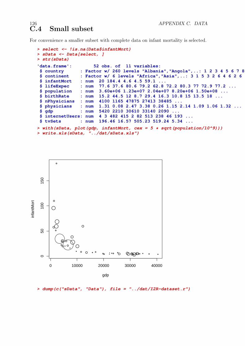
126 APPENDIX C. DATAC.4 Small subset
For convenience a smaller subset with complete data on infant mortality is selected.
> select <- !is.na(Data$infantMort)> sData <- Data[select, ]> str(sData)
'data.frame': 52 obs. of 11 variables:$ country : Factor w/ 260 levels "Albania","Angola",..: 1 2 3 4 5 6 7 8 9 10 ...$ continent : Factor w/ 6 levels "Africa","Asia",..: 3 1 5 3 2 6 4 6 2 6 ...$ infantMort : num 20 184.4 4.6 4.5 59.1 ...$ lifeExpec : num 77.6 37.6 80.6 79.2 62.8 72.2 80.3 77 72.9 77.2 ...$ population : num 3.60e+06 1.23e+07 2.04e+07 8.20e+06 1.50e+08 ...$ birthRate : num 15.2 44.5 12 8.7 29.4 16.3 10.8 15 13.5 18 ...$ nPhysicians : num 4100 1165 47875 27413 38485 ...$ physicians : num 1.31 0.08 2.47 3.38 0.26 1.15 2.14 1.09 1.06 1.32 ...$ gdp : num 5420 2210 30610 33140 2090 ...$ internetUsers: num 4 3 482 415 2 82 513 238 46 193 ...$ tvSets : num 196.46 16.57 505.23 519.24 5.34 ...
> with(sData, plot(gdp, infantMort, cex = 5 * sqrt(population/10^9)))> write.xls(sData, "../dat/sData.xls")
●
●
● ●
●
●
●●
●
●
● ●
●
●
●●●●
●
●
●
●● ● ●
●
●
●
●
●
●
●
●
●
●●
●
●
●
●
●
●●●
●
●
0 10000 20000 30000 40000
050
100
150
gdp
infa
ntM
ort
> dump(c("sData", "Data"), file = "../dat/I2R-dataset.r")

C.5. INTERESTING PACKAGES 127C.5 Interesting packages
prettyR Functions for conventionally formatted descriptive stats, and to format Routput as HTML
Hmisc Harrell Miscellaneous
MAAS Modern Applied Statistics with S

128 APPENDIX C. DATASessionInfo
Windows XP (build 2600) Service Pack 3
� R version 2.8.0 (2008-10-20), i386-pc-mingw32
� Locale: LC_COLLATE=Slovenian_Slovenia.1250;LC_CTYPE=Slovenian_Slovenia.1250;LC_MONETARY=Slovenian_Slovenia.1250;LC_NUMERIC=C;LC_TIME=Slovenian_Slovenia.1250
� Base packages: base, datasets, graphics, grDevices, methods, stats, utils
� Other packages: foreign 0.8-29, Hmisc 3.4-3, xlsReadWrite 1.3.2
� Loaded via a namespace (and not attached): cluster 1.11.11, grid 2.8.0, lat-tice 0.17-15
Revision Id: I2R.Rnw 9 2009-07-30 09:59:20Z ABlejec (c) A. Blejec


![NIB B L - Pakistan Credit Rating Agency(PACRA)€¦ · · 2015-09-30NEW [JUNE-15] PREVIOUS [JUNE-14] REPORT CONTENTS R 1. ... mainly comprising PICIC Asset Management ... NIB Bank](https://static.documents.pub/doc/80x56/5ac46e957f8b9a220b8cd23c/nib-b-l-pakistan-credit-rating-agencypacra-2015-09-30new-june-15-previous.jpg)


