+ All Categories
Home > Documents > introduction-to-regression-analysis - Computer Science · introduction-to-regression-analysis June...

introduction-to-regression-analysis - Computer Science · introduction-to-regression-analysis June...

Date post: 25-May-2020
Category:
Upload: others
View: 25 times
Download: 0 times
Share this document with a friend
23
introduction-to-regression-analysis June 3, 2019 1 Regression analysis of medical data Antti Honkela, antti.honkela@helsinki.fi We have earlier done linear regression using scikit-learn. In this project work, however, we will use the Statsmodels library. This is because Statsmodels has better statistical tools. In addition, it works better with Pandas’ DataFrames, since it can specify the relation between the dependent and independent variables using a formula notation of column names of a DataFrame. Below is an example of a formula: formula = "Y ~ X1 + X2" So, the formula is given as a string where the on the left side of the ~ character is the dependent variable, and on the right side the independent variables, separated using the + character. In this example the variable names Y, X1, and X2 refer to columns of a DataFrame. [2]: import numpy as np import matplotlib.pyplot as plt import statsmodels import statsmodels.api as sm import statsmodels.formula.api as smf # plots a line given an intercept and a slope from statsmodels.graphics.regressionplots import abline_plot import pandas as pd 2 Multi-variable linear regression Topics: - Multiple linear regression - Use of background variables to rectify regression - Interac- tions between variables - Choosing variables - Interpretation of estimation results Multi-variable linear regression is used to model phenomena that depend on multiple vari- ables. It can be used to adjust the model to consider confounding variables. It can also be used to recognize factors that have significant effect on a phenomenon. Learning targets: - Fit multi-variable linear regression models in Python - Rectify regression models with background variables, and analyse the rectified models - Understand the principle of variable choosing - Understand most important restrictions of multiple linear regression models Simple linear regression model is y i = α + βx i + ϵ i , 1
Transcript

introduction-to-regression-analysis

June 3, 2019

1 Regression analysis of medical data

Antti Honkela, [email protected] have earlier done linear regression using scikit-learn. In this project work, however, we will

use the Statsmodels library. This is because Statsmodels has better statistical tools. In addition,it works better with Pandas’ DataFrames, since it can specify the relation between the dependentand independent variables using a formula notation of column names of a DataFrame. Below isan example of a formula:

formula = "Y ~ X1 + X2"

So, the formula is given as a string where the on the left side of the ~ character is the dependentvariable, and on the right side the independent variables, separated using the + character. In thisexample the variable names Y, X1, and X2 refer to columns of a DataFrame.

[2]: import numpy as npimport matplotlib.pyplot as pltimport statsmodelsimport statsmodels.api as smimport statsmodels.formula.api as smf# plots a line given an intercept and a slopefrom statsmodels.graphics.regressionplots import abline_plotimport pandas as pd

2 Multi-variable linear regression

Topics: - Multiple linear regression - Use of background variables to rectify regression - Interac-tions between variables - Choosing variables - Interpretation of estimation results

Multi-variable linear regression is used to model phenomena that depend on multiple vari-ables. It can be used to adjust the model to consider confounding variables. It can also be used torecognize factors that have significant effect on a phenomenon.

Learning targets: - Fit multi-variable linear regression models in Python - Rectify regressionmodels with background variables, and analyse the rectified models - Understand the principle ofvariable choosing - Understand most important restrictions of multiple linear regression models

Simple linear regression model is

yi = α + βxi + ϵi,

1

where - yi is the explained variable - xi is the explanatory variable - β is the regression coefficient- α is the constant term (intercept) - ϵi is the residual.

Multi-variable linear regression model (or multiple liner regression model) is

yi = α + β1xi1 + · · ·+ βpxip + ϵi

• yi is the explained variable• xij are the explanatory variables j = 1, . . . , p

• β j are the regression coefficients• α is the constant term (intercept)• ϵi is the residual.

The data can be represented as a design matrix that has variables as columns and observationsas rows.

X =

x11 x12 · · · x1px21 x22 · · · x2p

......

. . ....

xn1 xn2 · · · xnp

The whole regression model in a matrix form is

y = α1 + Xβ + ffl

y1y2...

yn

= α

11...1

+

x11 x12 · · · x1px21 x22 · · · x2p

......

. . ....

xn1 xn2 · · · xnp

β1

...βp

+ ffl

yi = α + β1xi1 + · · ·+ βpxip + ϵi

Or equivalently

y =(1 X

) (αβ

)+ ffl

y1y2...

yn

=

1 x11 x12 · · · x1p1 x21 x22 · · · x2p...

......

. . ....

1 xn1 xn2 · · · xnp

αβ1β2...

βp

+ ffl

yi = α + β1xi1 + · · ·+ βpxip + ϵi

Or as Python expression:

y == np.concatenate([np.ones((len(x), 1)), X], axis=1) @ fit.params

2

2.0.1 An example using the Framingham Heart study

Data from the Framingham Heart study. In 1948, the study was initiated to identify the commonfactors or characteristics that contribute to CVD by following its development over time in groupof participants who had not yet developed overt symptoms of CVD or suffered a heart attack orstroke. The researchers recruited 5,209 men and women between the ages of 30 and 62 from thetown of Framingham, Massachusetts. Every two years, a series of extensive physical examinationsand lifestyle interviews were conducted. This data set is subset of the Framingham Heart studydata. The data is stored as 14 columns. Each row represents a single subject.

[3]: # Load the datafram = pd.read_csv('fram.txt', sep='\t')fram.head()

[3]: ID SEX AGE FRW SBP SBP10 DBP CHOL CIG CHD YRS_CHD DEATH \0 4988 female 57 135 186 NaN 120 150 0 1 pre 71 3001 female 60 123 165 NaN 100 167 25 0 16 102 5079 female 54 115 140 NaN 90 213 5 0 8 83 5162 female 52 102 170 NaN 104 280 15 0 10 74 4672 female 45 99 185 NaN 105 326 20 0 8 10

YRS_DTH CAUSE0 11 unknown1 17 unknown2 13 unknown3 11 unknown4 17 unknown

ID Explanation

SEX GenderAGE Age at the start of the studyFRW Weight in relation to groups medianSBP Systolic Blood PressureDBP Diastolic Blood PressureCHOL Cholestherol levelCIG Smoking (cigarets per day)

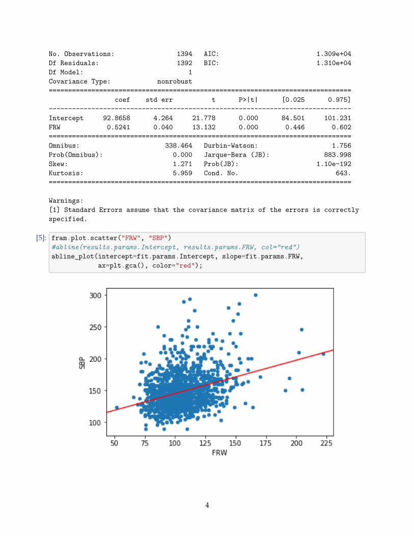
As an example, let’s predict the systolic blood pressure using the weight.[4]: fit = smf.ols('SBP ~ FRW', data=fram).fit()

print(fit.summary())

OLS Regression Results==============================================================================Dep. Variable: SBP R-squared: 0.110Model: OLS Adj. R-squared: 0.110Method: Least Squares F-statistic: 172.5Date: Mon, 03 Jun 2019 Prob (F-statistic): 3.18e-37Time: 19:01:30 Log-Likelihood: -6542.3

3

No. Observations: 1394 AIC: 1.309e+04Df Residuals: 1392 BIC: 1.310e+04Df Model: 1Covariance Type: nonrobust==============================================================================

coef std err t P>|t| [0.025 0.975]------------------------------------------------------------------------------Intercept 92.8658 4.264 21.778 0.000 84.501 101.231FRW 0.5241 0.040 13.132 0.000 0.446 0.602==============================================================================Omnibus: 338.464 Durbin-Watson: 1.756Prob(Omnibus): 0.000 Jarque-Bera (JB): 883.998Skew: 1.271 Prob(JB): 1.10e-192Kurtosis: 5.959 Cond. No. 643.==============================================================================

Warnings:[1] Standard Errors assume that the covariance matrix of the errors is correctlyspecified.

[5]: fram.plot.scatter("FRW", "SBP")#abline(results.params.Intercept, results.params.FRW, col="red")abline_plot(intercept=fit.params.Intercept, slope=fit.params.FRW,

ax=plt.gca(), color="red");

4

Next we rectify the model using background variables.Assumptions of a regression model: 1. Relevance of data to the research question 2. Linearity

and additivity 3. Independence of residuals 4. Constancy of variance of residuals 5. Normaldistribution of residuals

Do these hold now?In multiple-variable regression we add the background variables as explanators. Note: this

rectification is linear an additive. In principle one should include all background variables, butestimation using too many variable can be unreliable.

Let’s first consider a binary variable (gender).[6]: # Incorporate the gender

fit=smf.ols('SBP ~ FRW + SEX', data=fram).fit()print(fit.summary())

OLS Regression Results==============================================================================Dep. Variable: SBP R-squared: 0.118Model: OLS Adj. R-squared: 0.117Method: Least Squares F-statistic: 92.94Date: Mon, 03 Jun 2019 Prob (F-statistic): 1.31e-38Time: 19:01:30 Log-Likelihood: -6536.3No. Observations: 1394 AIC: 1.308e+04Df Residuals: 1391 BIC: 1.309e+04Df Model: 2Covariance Type: nonrobust===============================================================================

coef std err t P>|t| [0.025 0.975]-------------------------------------------------------------------------------Intercept 97.6608 4.466 21.866 0.000 88.899 106.422SEX[T.male] -4.9701 1.432 -3.470 0.001 -7.780 -2.161FRW 0.5010 0.040 12.431 0.000 0.422 0.580==============================================================================Omnibus: 330.964 Durbin-Watson: 1.768Prob(Omnibus): 0.000 Jarque-Bera (JB): 851.938Skew: 1.249 Prob(JB): 1.01e-185Kurtosis: 5.902 Cond. No. 680.==============================================================================

Warnings:[1] Standard Errors assume that the covariance matrix of the errors is correctlyspecified.

Next we visualize men separately from women.[7]: fram.plot.scatter("FRW", "SBP")

int1 = fit.params.Intercept + fit.params["SEX[T.male]"]int2 = fit.params.Interceptslope=fit.params.FRW

5

abline_plot(intercept=int1, slope=slope, ax=plt.gca(), color="blue",␣↪→label="male")

abline_plot(intercept=int2, slope=slope, ax=plt.gca(), color="red",␣↪→label="female")

plt.legend();

The previous model acknowledged the gender in the intercept, but not in the slope. We im-prove the model by adding an interaction term FRW:SEX. Interaction is the product of the two vari-ables. (Note that in these dependence formulas A * B is an abbreviation for A + B + A:B. The *character is not often used in the formulas.)

[8]: # Include both gender and its interaction with the weightfit2=smf.ols('SBP ~ FRW + SEX + FRW:SEX', data=fram).fit()print(fit2.summary())

OLS Regression Results==============================================================================Dep. Variable: SBP R-squared: 0.118Model: OLS Adj. R-squared: 0.116Method: Least Squares F-statistic: 61.92Date: Mon, 03 Jun 2019 Prob (F-statistic): 1.42e-37Time: 19:01:30 Log-Likelihood: -6536.3No. Observations: 1394 AIC: 1.308e+04Df Residuals: 1390 BIC: 1.310e+04Df Model: 3

6

Covariance Type: nonrobust===================================================================================

coef std err t P>|t| [0.0250.975]-----------------------------------------------------------------------------------Intercept 98.0027 5.324 18.408 0.000 87.559108.446SEX[T.male] -6.0457 9.219 -0.656 0.512 -24.13012.038FRW 0.4979 0.048 10.288 0.000 0.4030.593FRW:SEX[T.male] 0.0103 0.087 0.118 0.906 -0.1610.182==============================================================================Omnibus: 331.026 Durbin-Watson: 1.768Prob(Omnibus): 0.000 Jarque-Bera (JB): 852.312Skew: 1.250 Prob(JB): 8.37e-186Kurtosis: 5.903 Cond. No. 1.66e+03==============================================================================

Warnings:[1] Standard Errors assume that the covariance matrix of the errors is correctlyspecified.[2] The condition number is large, 1.66e+03. This might indicate that there arestrong multicollinearity or other numerical problems.

[10]: # Renormalize to ease interpretation of the model parametersfram["sAGE"] = rescale(fram.AGE)fram["sFRW"] = rescale(fram.FRW)fram["sCHOL"] = rescale(fram.CHOL)fram["sCIG"] = rescale(fram.CIG)# Note: No need to scale the variable SEX

[11]: # Now with renormalized variablesfit3=smf.ols('SBP ~ sFRW + SEX + sFRW:SEX', data=fram).fit()print(fit3.summary())

OLS Regression Results==============================================================================Dep. Variable: SBP R-squared: 0.118Model: OLS Adj. R-squared: 0.116Method: Least Squares F-statistic: 61.92Date: Mon, 03 Jun 2019 Prob (F-statistic): 1.42e-37Time: 19:01:30 Log-Likelihood: -6536.3No. Observations: 1394 AIC: 1.308e+04Df Residuals: 1390 BIC: 1.310e+04

7

Df Model: 3Covariance Type: nonrobust====================================================================================

coef std err t P>|t| [0.0250.975]------------------------------------------------------------------------------------Intercept 150.4587 0.984 152.940 0.000 148.529152.389SEX[T.male] -4.9569 1.437 -3.449 0.001 -7.776-2.138sFRW 17.6762 1.718 10.288 0.000 14.30621.047sFRW:SEX[T.male] 0.3669 3.106 0.118 0.906 -5.7276.461==============================================================================Omnibus: 331.026 Durbin-Watson: 1.768Prob(Omnibus): 0.000 Jarque-Bera (JB): 852.312Skew: 1.250 Prob(JB): 8.37e-186Kurtosis: 5.903 Cond. No. 5.27==============================================================================

Warnings:[1] Standard Errors assume that the covariance matrix of the errors is correctlyspecified.

[12]: p=fit3.paramsfram.plot.scatter("sFRW", "SBP")#abline(p.Intercept + p["SEX[T.male]"],# p.sFRW + p["sFRW:SEX[T.male]"], col="blue", label="male")#abline(p.Intercept, p.sFRW, col="red", label="female")int1 = p.Intercept + p["SEX[T.male]"]int2 = p.Interceptslope1 = p.sFRW + p["sFRW:SEX[T.male]"]slope2 = p.sFRWabline_plot(intercept=int1, slope=slope1, ax=plt.gca(), color="blue",␣

↪→label="male")abline_plot(intercept=int2, slope=slope2, ax=plt.gca(), color="red",␣

↪→label="female")plt.legend();

8

2.1 Background variables

ID Explanation

SEX GenderAGE Age at the start of the studyFRW Weight in relation to groups medianSBP Systolic Blood PressureDBP Diastolic Blood PressureCHOL Cholestherol levelCIG Smoking (cigarets per day)

Next we add a continuous background variable: cholesterol.[13]: fit4=smf.ols('SBP ~ sFRW + SEX + sFRW:SEX + sCHOL', data=fram).fit()

print(fit4.summary())

OLS Regression Results==============================================================================Dep. Variable: SBP R-squared: 0.125Model: OLS Adj. R-squared: 0.123Method: Least Squares F-statistic: 49.75Date: Mon, 03 Jun 2019 Prob (F-statistic): 3.67e-39Time: 19:01:30 Log-Likelihood: -6530.4

9

No. Observations: 1394 AIC: 1.307e+04Df Residuals: 1389 BIC: 1.310e+04Df Model: 4Covariance Type: nonrobust====================================================================================

coef std err t P>|t| [0.0250.975]------------------------------------------------------------------------------------Intercept 150.0166 0.988 151.776 0.000 148.078151.955SEX[T.male] -4.0700 1.455 -2.798 0.005 -6.923-1.216sFRW 17.7594 1.712 10.375 0.000 14.40221.117sFRW:SEX[T.male] -0.1272 3.098 -0.041 0.967 -6.2045.950sCHOL 4.9197 1.433 3.433 0.001 2.1087.731==============================================================================Omnibus: 327.586 Durbin-Watson: 1.774Prob(Omnibus): 0.000 Jarque-Bera (JB): 843.566Skew: 1.237 Prob(JB): 6.64e-184Kurtosis: 5.899 Cond. No. 5.28==============================================================================

Warnings:[1] Standard Errors assume that the covariance matrix of the errors is correctlyspecified.

[14]: # Add interactions between variablesfit4=smf.ols('SBP ~ sFRW + SEX + sFRW:SEX + sCHOL + sCHOL:sFRW + sCHOL:SEX',

data=fram).fit()print(fit4.summary())

OLS Regression Results==============================================================================Dep. Variable: SBP R-squared: 0.127Model: OLS Adj. R-squared: 0.123Method: Least Squares F-statistic: 33.58Date: Mon, 03 Jun 2019 Prob (F-statistic): 5.65e-38Time: 19:01:30 Log-Likelihood: -6529.2No. Observations: 1394 AIC: 1.307e+04Df Residuals: 1387 BIC: 1.311e+04Df Model: 6Covariance Type: nonrobust

10

=====================================================================================

coef std err t P>|t| [0.0250.975]-------------------------------------------------------------------------------------Intercept 149.9420 0.994 150.850 0.000 147.992151.892SEX[T.male] -4.0980 1.455 -2.816 0.005 -6.953-1.243sFRW 17.9750 1.718 10.466 0.000 14.60621.344sFRW:SEX[T.male] 0.2760 3.108 0.089 0.929 -5.8216.373sCHOL 5.5034 1.861 2.958 0.003 1.8539.154sCHOL:SEX[T.male] -1.3225 2.939 -0.450 0.653 -7.0874.442sCHOL:sFRW 3.9052 2.741 1.425 0.154 -1.4719.282==============================================================================Omnibus: 318.099 Durbin-Watson: 1.769Prob(Omnibus): 0.000 Jarque-Bera (JB): 798.422Skew: 1.212 Prob(JB): 4.22e-174Kurtosis: 5.805 Cond. No. 5.32==============================================================================

Warnings:[1] Standard Errors assume that the covariance matrix of the errors is correctlyspecified.

Normalized data (rescale) allows analysis of the importance of variables. An interpretation:how much does a change of 2*standard deviation affect the explained variable. In the followingwe visualize women with either low, medium or high cholestherol.

[15]: p=fit4.params#fram.plot.scatter("sFRW", "SBP")fram[fram.SEX=="female"].plot.scatter("sFRW", "SBP")abline_plot(intercept=p.Intercept - p["sCHOL"], slope=p.sFRW - p["sCHOL:sFRW"],

ax=plt.gca(), color="blue", label="low")abline_plot(intercept=p.Intercept, slope=p.sFRW,

ax=plt.gca(), color="magenta", label="mid")abline_plot(intercept=p.Intercept + p["sCHOL"], slope=p.sFRW + p["sCHOL:sFRW"],

ax=plt.gca(), color="red", label="high")plt.legend();

11

Below is the same analysis but in separate visualizations.[16]: fig, ax = plt.subplots(1,3, subplot_kw={"xlim": (-1.6, 3.3), "ylim": (80,310),

"xlabel": "sFRW", "ylabel": "SBP"},figsize=(14, 4))

ax[0].scatter(fram.sFRW[(fram.SEX=="female") & (fram.sCHOL < -0.5)],fram.SBP[(fram.SEX=="female") & (fram.sCHOL < -0.5)])

abline_plot(p.Intercept - p["sCHOL"],p.sFRW - p["sCHOL:sFRW"], color="blue", label="low", ax=ax[0])

ax[0].set_title("female, low CHOL")

ax[1].scatter(fram.sFRW[(fram.SEX=="female") & (fram.sCHOL > -0.5) &(fram.sCHOL < 0.5)],

fram.SBP[(fram.SEX=="female") & (fram.sCHOL > -0.5) &(fram.sCHOL < 0.5)])

abline_plot(p.Intercept, p.sFRW, color="magenta", label="mid", ax=ax[1])ax[1].set_title("female, mid CHOL")

ax[2].scatter(fram.sFRW[(fram.SEX=="female") & (fram.sCHOL > 0.5)],fram.SBP[(fram.SEX=="female") & (fram.sCHOL > 0.5)])

abline_plot(p.Intercept + p["sCHOL"],p.sFRW + p["sCHOL:sFRW"], color="red", label="high", ax=ax[2])

ax[2].set_title("female, high CHOL")

[16]: Text(0.5, 1.0, 'female, high CHOL')

12

2.1.1 Prediction and generalization

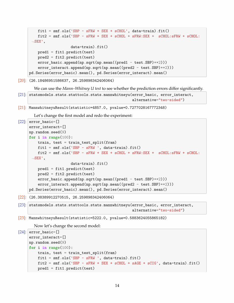
Model’s predictive accuracy in the data it was learned from does not give a good picture of itspredictive capabilities: the model can be overfitted. A better estimate for the predictive accuracycan be obtained using cross validation: 1. Divide the data into parts for fitting and for validation2. The model is fitted in a part of the data (training data) 3. The models is tested on another partof the data (test data). Then prediction error is computed. 4. This is repeated for a wanted numberof divisions of the data

One model:[18]: train, test = train_test_split(fram) # Split the date into two␣

↪→partsfit = smf.ols('SBP ~ sFRW + SEX + sCHOL', data=train).fit() # Fit the modelpred = fit.predict(test) # Compute predictionsrmse = np.sqrt(np.mean((pred - test.SBP)**2)) # Root mean square errorrmse

[18]: 25.854547340698

Another model:[19]: train, test = train_test_split(fram)

fit = smf.ols('SBP ~ sFRW + SEX + sCHOL + sFRW:SEX + sCHOL:sFRW + sCHOL:SEX',data=train).fit()

pred = fit.predict(test)rmse = np.sqrt(np.mean((pred - test.SBP)**2))rmse

[19]: 27.144351010633336

Let’s repeat this random data splitting 100 times for both models and compute the averageRMSEs:

[20]: error_basic=[]error_interact=[]np.random.seed(9)for i in range(100):

train, test = train_test_split(fram)

13

fit1 = smf.ols('SBP ~ sFRW + SEX + sCHOL', data=train).fit()fit2 = smf.ols('SBP ~ sFRW + SEX + sCHOL + sFRW:SEX + sCHOL:sFRW + sCHOL:

↪→SEX',data=train).fit()

pred1 = fit1.predict(test)pred2 = fit2.predict(test)error_basic.append(np.sqrt(np.mean((pred1 - test.SBP)**2)))error_interact.append(np.sqrt(np.mean((pred2 - test.SBP)**2)))

pd.Series(error_basic).mean(), pd.Series(error_interact).mean()

[20]: (26.18486951586637, 26.259898342406064)

We can use the Mann–Whitney U test to see whether the prediction errors differ significantly.[21]: statsmodels.stats.stattools.stats.mannwhitneyu(error_basic, error_interact,

alternative="two-sided")

[21]: MannwhitneyuResult(statistic=4857.0, pvalue=0.7277028167772348)

Let’s change the first model and redo the experiment:[22]: error_basic=[]

error_interact=[]np.random.seed(9)for i in range(100):

train, test = train_test_split(fram)fit1 = smf.ols('SBP ~ sFRW ', data=train).fit()fit2 = smf.ols('SBP ~ sFRW + SEX + sCHOL + sFRW:SEX + sCHOL:sFRW + sCHOL:

↪→SEX',data=train).fit()

pred1 = fit1.predict(test)pred2 = fit2.predict(test)error_basic.append(np.sqrt(np.mean((pred1 - test.SBP)**2)))error_interact.append(np.sqrt(np.mean((pred2 - test.SBP)**2)))

pd.Series(error_basic).mean(), pd.Series(error_interact).mean()

[22]: (26.38389912270515, 26.259898342406064)

[23]: statsmodels.stats.stattools.stats.mannwhitneyu(error_basic, error_interact,alternative="two-sided")

[23]: MannwhitneyuResult(statistic=5222.0, pvalue=0.5883624055865182)

Now let’s change the second model:[24]: error_basic=[]

error_interact=[]np.random.seed(9)for i in range(100):

train, test = train_test_split(fram)fit1 = smf.ols('SBP ~ sFRW ', data=train).fit()fit2 = smf.ols('SBP ~ sFRW + SEX + sCHOL + sAGE + sCIG', data=train).fit()pred1 = fit1.predict(test)

14

pred2 = fit2.predict(test)error_basic.append(np.sqrt(np.mean((pred1 - test.SBP)**2)))error_interact.append(np.sqrt(np.mean((pred2 - test.SBP)**2)))

pd.Series(error_basic).mean(), pd.Series(error_interact).mean()

[24]: (26.38389912270515, 25.924525100203073)

[25]: statsmodels.stats.stattools.stats.mannwhitneyu(error_basic, error_interact,alternative="two-sided")

[25]: MannwhitneyuResult(statistic=5742.0, pvalue=0.0700213003206784)

3 Logistic regression

Topics:

• Logistic regression model• Classification problems

Learning targets:

• Fit logistic regression models with Python• Interpret the estimated regression models

3.1 Regression model is transformations of variables

Multi-variable linear regression model:

yi = α + β1xi1 + · · ·+ βpxip + ϵi

The model is very flexible with respect to the variables xij and yi: the variables need not bedirect observations, for example the interaction terms like SEX:sWHP. Also transformations of vari-ables are permitted, for example SBP ~ log(FRW) + sFRW + SEX + SEX:sFRW.

For example, logarithm transform is often useful for variables, whose range is large and whoseeffect can be expected to saturate. An example: log(SBP) ~ log(FRW) + SEX + SEX:log(FRW)

SBP = αFRWβ1 exp(SEX)β2 FRWSEX·β3

3.2 Binary target variable (classification)

It is not sensible to try to predict a binary variable directly using linear regression. In general,we want to predict p(yi = TRUE | X). In linear regression the possible values are in the interval(−∞, ∞), whereas probabilities are in the interval [0, 1]. The idea is to transform the unrestrictedpredictions to probabilities.

[26]: def logistic(x):return 1.0 / (1.0 + np.exp(-x))

[27]: X=np.linspace(-8, 8, 100)plt.plot(X, logistic(X));

15

logit−1(x) =1

1 + exp(−x)Logistic transform is non-linear: same change in input produces different changes in probabil-

ities. The speed of change is at its largest at the point x = 0 : f ′(0) = 1/4. Logistic regression is themost common tool for classification. It can also be used to recognize variables that are importantto the classification.

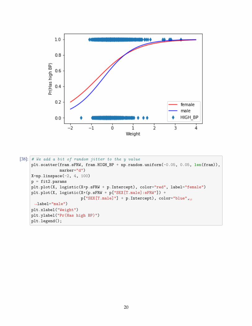
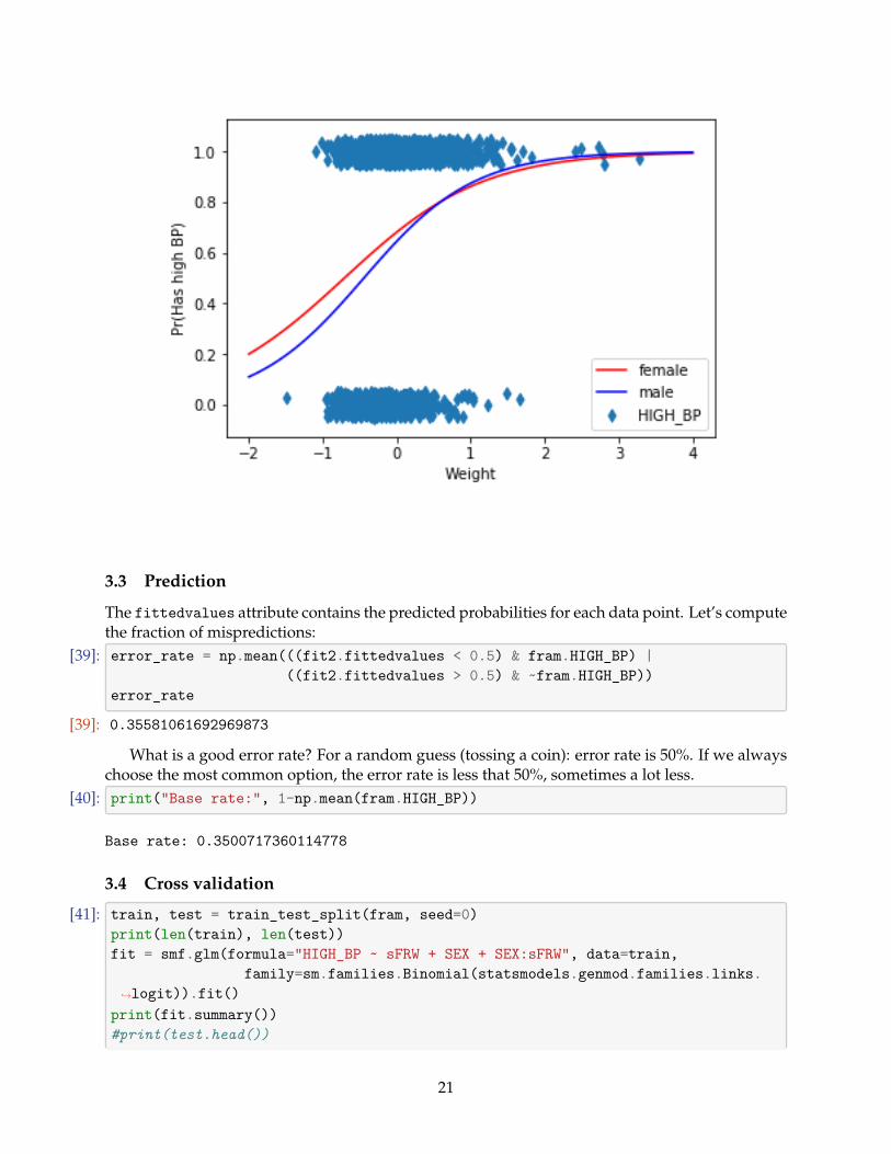
Let’s continue with the fram data. First we define a diagnose for high blood pressure.[28]: fram["HIGH_BP"] = (fram.SBP >= 140) | (fram.DBP >= 90)

fram.HIGH_BP.head()

[28]: 0 True1 True2 True3 True4 TrueName: HIGH_BP, dtype: bool

[29]: fram.HIGH_BP.value_counts()

[29]: True 906False 488Name: HIGH_BP, dtype: int64

[30]: fram.HIGH_BP = fram.HIGH_BP.map(int)

Note that for boolean variables we use type int here instead of bool, because we want to makethe encoding of booleans as integers explicit: 0 for False and 1 for True. (The implicit encodingof booleans as integers in statsmodels library is unfortunately inconsistent.)

16

[31]: fram.HIGH_BP.mean() # Fraction of observations with this diagnose

[31]: 0.6499282639885222

[32]: fram.head()

[32]: ID SEX AGE FRW SBP SBP10 DBP CHOL CIG CHD YRS_CHD DEATH \0 4988 female 57 135 186 NaN 120 150 0 1 pre 71 3001 female 60 123 165 NaN 100 167 25 0 16 102 5079 female 54 115 140 NaN 90 213 5 0 8 83 5162 female 52 102 170 NaN 104 280 15 0 10 74 4672 female 45 99 185 NaN 105 326 20 0 8 10

YRS_DTH CAUSE sAGE sFRW sCHOL sCIG HIGH_BP0 11 unknown 0.477764 0.834668 -0.914016 -0.346569 11 17 unknown 0.791473 0.496687 -0.730446 0.732493 12 13 unknown 0.164056 0.271367 -0.233727 -0.130757 13 11 unknown -0.045083 -0.094779 0.489755 0.300868 14 17 unknown -0.777070 -0.179274 0.986475 0.516680 1

Let’s fit a logistic regression model:[33]: fit1 = smf.glm(formula="HIGH_BP ~ FRW", data=fram,

family=sm.families.Binomial(statsmodels.genmod.families.links.↪→logit)).fit()

fit1.summary()

[33]: <class 'statsmodels.iolib.summary.Summary'>"""

Generalized Linear Model Regression Results==============================================================================Dep. Variable: HIGH_BP No. Observations: 1394Model: GLM Df Residuals: 1392Model Family: Binomial Df Model: 1Link Function: logit Scale: 1.0000Method: IRLS Log-Likelihood: -858.64Date: Mon, 03 Jun 2019 Deviance: 1717.3Time: 19:01:38 Pearson chi2: 1.39e+03No. Iterations: 4 Covariance Type: nonrobust==============================================================================

coef std err z P>|z| [0.025 0.975]------------------------------------------------------------------------------Intercept -2.8912 0.404 -7.158 0.000 -3.683 -2.100FRW 0.0339 0.004 8.650 0.000 0.026 0.042=============================================================================="""

[34]: fit1.params

[34]: Intercept -2.891166FRW 0.033852

17

dtype: float64

The R2 is not sensible now. Instead, we use deviance, which measures the error. Smaller value isbetter. The coefficients are mostly like in linear regression. Also, the significance interpretation isthe same. Coefficient β: change of one unit in a variable causes a change in the probability whichis at most β/4.

[35]: # Visualization of the modelplt.scatter(fram.FRW, fram.HIGH_BP, marker="d")X=np.linspace(40, 235, 100)plt.plot(X, logistic(X*fit1.params.FRW + fit1.params.Intercept))plt.xlabel("FRW")plt.ylabel("HIGH_BP")

[35]: Text(0, 0.5, 'HIGH_BP')

Next we add the gender and its interaction to the model:[36]: fit2 = smf.glm(formula="HIGH_BP ~ sFRW + SEX + SEX:sFRW", data=fram,

family=sm.families.Binomial()).fit()fit2.summary()

[36]: <class 'statsmodels.iolib.summary.Summary'>"""

Generalized Linear Model Regression Results==============================================================================Dep. Variable: HIGH_BP No. Observations: 1394Model: GLM Df Residuals: 1390

18

Model Family: Binomial Df Model: 3Link Function: logit Scale: 1.0000Method: IRLS Log-Likelihood: -856.87Date: Mon, 03 Jun 2019 Deviance: 1713.7Time: 19:01:38 Pearson chi2: 1.39e+03No. Iterations: 4 Covariance Type: nonrobust====================================================================================

coef std err z P>|z| [0.0250.975]------------------------------------------------------------------------------------Intercept 0.7631 0.082 9.266 0.000 0.6020.925SEX[T.male] -0.1624 0.120 -1.350 0.177 -0.3980.073sFRW 1.0738 0.176 6.095 0.000 0.7281.419SEX[T.male]:sFRW 0.2709 0.287 0.943 0.346 -0.2920.834===================================================================================="""

[37]: plt.scatter(fram.sFRW, fram.HIGH_BP, marker="d")X=np.linspace(-2, 4, 100)p = fit2.paramsplt.plot(X, logistic(X*p.sFRW + p.Intercept), color="red", label="female")plt.plot(X, logistic(X*(p.sFRW + p["SEX[T.male]:sFRW"]) +

p["SEX[T.male]"] + p.Intercept), color="blue",␣↪→label="male")

plt.xlabel("Weight")plt.ylabel("Pr(Has high BP)")plt.legend();

19

[38]: # We add a bit of random jitter to the y valueplt.scatter(fram.sFRW, fram.HIGH_BP + np.random.uniform(-0.05, 0.05, len(fram)),

marker="d")X=np.linspace(-2, 4, 100)p = fit2.paramsplt.plot(X, logistic(X*p.sFRW + p.Intercept), color="red", label="female")plt.plot(X, logistic(X*(p.sFRW + p["SEX[T.male]:sFRW"]) +

p["SEX[T.male]"] + p.Intercept), color="blue",␣↪→label="male")

plt.xlabel("Weight")plt.ylabel("Pr(Has high BP)")plt.legend();

20

3.3 Prediction

The fittedvalues attribute contains the predicted probabilities for each data point. Let’s computethe fraction of mispredictions:

[39]: error_rate = np.mean(((fit2.fittedvalues < 0.5) & fram.HIGH_BP) |((fit2.fittedvalues > 0.5) & ~fram.HIGH_BP))

error_rate

[39]: 0.35581061692969873

What is a good error rate? For a random guess (tossing a coin): error rate is 50%. If we alwayschoose the most common option, the error rate is less that 50%, sometimes a lot less.

[40]: print("Base rate:", 1-np.mean(fram.HIGH_BP))

Base rate: 0.3500717360114778

3.4 Cross validation

[41]: train, test = train_test_split(fram, seed=0)print(len(train), len(test))fit = smf.glm(formula="HIGH_BP ~ sFRW + SEX + SEX:sFRW", data=train,

family=sm.families.Binomial(statsmodels.genmod.families.links.↪→logit)).fit()

print(fit.summary())#print(test.head())

21

pred = fit.predict(test, transform=True)#print(pred.describe())#print("Min:", pred.min())#print("Max:", pred.max())error_rate = np.mean(((pred < 0.5) & (test.HIGH_BP==1)) |

((pred > 0.5) & (test.HIGH_BP==0)))print(error_rate, 1 - test.HIGH_BP.mean())

1115 279Generalized Linear Model Regression Results

==============================================================================Dep. Variable: HIGH_BP No. Observations: 1115Model: GLM Df Residuals: 1111Model Family: Binomial Df Model: 3Link Function: logit Scale: 1.0000Method: IRLS Log-Likelihood: -689.76Date: Mon, 03 Jun 2019 Deviance: 1379.5Time: 19:01:39 Pearson chi2: 1.11e+03No. Iterations: 4 Covariance Type: nonrobust====================================================================================

coef std err z P>|z| [0.0250.975]------------------------------------------------------------------------------------Intercept 0.8008 0.092 8.752 0.000 0.6210.980SEX[T.male] -0.2329 0.134 -1.743 0.081 -0.4950.029sFRW 0.9641 0.197 4.895 0.000 0.5781.350SEX[T.male]:sFRW 0.1760 0.315 0.558 0.577 -0.4420.794====================================================================================0.35125448028673834 0.36200716845878134

[42]: error_model=[]error_null=[]np.random.seed(1)for i in range(100):

train, test = train_test_split(fram)fit = smf.glm(formula="HIGH_BP ~ sFRW + SEX + SEX:sFRW", data=train,

family=sm.families.Binomial(statsmodels.genmod.families.↪→links.logit)).fit()

#print(model.summary())pred = fit.predict(test, transform=True)

22

error_rate = np.mean(((pred < 0.5) & (test.HIGH_BP==1)) |((pred > 0.5) & (test.HIGH_BP==0)))

error_model.append(error_rate)error_null.append((1 - test.HIGH_BP).mean())

#for model, null in zip(error_model, error_null):# print(model, null)pd.Series(error_model).mean(), pd.Series(error_null).mean()

[42]: (0.3520071684587814, 0.3488530465949821)

Test to see whether the results are significantly different:[43]: statsmodels.stats.stattools.stats.mannwhitneyu(error_model, error_null,

alternative="two-sided")

[43]: MannwhitneyuResult(statistic=5312.5, pvalue=0.44539961439180353)

Let’s define another diagnose:[44]: fram["HIGH_BP2"] = (fram.SBP > 140) | (fram.DBP > 90)

fram["HIGH_BP2"] = fram["HIGH_BP2"].map(int)fram["HIGH_BP2"].mean()

[44]: 0.56025824964132

[45]: error_model=[]error_null=[]np.random.seed(9)for i in range(100):

train, test = train_test_split(fram)fit = smf.glm(formula="HIGH_BP2 ~ sFRW + SEX + SEX:sFRW", data=train,

family=sm.families.Binomial()).fit()#print(model.summary())pred = fit.predict(test)error_rate = np.mean(((pred < 0.5) & (test.HIGH_BP2==1)) |

((pred > 0.5) & (test.HIGH_BP2==0)))error_model.append(error_rate)error_null.append((1-test.HIGH_BP2).mean())

#for model, null in zip(error_model, error_null):# print(model, null)pd.Series(error_model).mean(), pd.Series(error_null).mean()

[45]: (0.3860931899641578, 0.4403942652329749)

Test again:[46]: statsmodels.stats.stattools.stats.mannwhitneyu(error_model, error_null,

alternative="two-sided")

[46]: MannwhitneyuResult(statistic=525.0, pvalue=7.3782255350127615e-28)

23


Recommended