Introduction to RooFit - Istituto Nazionale di Fisica...

Introduction to RooFit

1. Introduction and overview

2. Creation and basic use of models

3. Addition and Convolution

4. Common Fitting problems

W. Verkerke (NIKHEF)

4. Common Fitting problems

5. Multidimensional and Conditional models

6. Fit validation and toy MC studies

7. Constructing joint models

8. Working with the Likelihood, including systematic errors

9. Intervals & Limits

Constructing joint models7

Wouter Verkerke, NIKHEF

joint models7• Using discrete variable to classify data• Simultaneous fits on multiple datasets

Datasets and discrete observables

• Discrete observables play an important role in management of datasets– Useful to classify ‘sub datasets’ inside datasets

– Can collapse multiple, logically separate datasets into a single dataset by adding them and labeling the source with a discrete observable

– Allows to express operations such a simultaneous fits as operation on a single dataset


Dataset A

X

5.0

3.7

1.2

4.3 Dataset B

X

5.0

3.7

1.2

Dataset A+B

X source

5.0 A

3.7 A

1.2 A

4.3 A

5.0 B

3.7 B

1.2 B

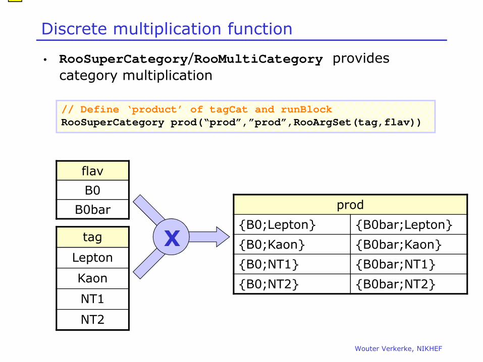
Discrete variables in RooFit – RooCategory

• Properties of RooCategory variables– Finite set of named states → self documenting

– Optional integer code associated with each state

// Define a cat. with explicitly numbered statesw.factory(“b0flav[B0=-1,B0bar=1]”) ;

// Define a category with labels only


• Used for classification of data, or to describe occasional discrete fundamental observable (e.g. B0 flavor)

// Define a category with labels onlyw.factory(“tagCat[Lepton,Kaon,NT1,NT2]”) ;w.factory(“sample[CPV,BMixing]”) ;

Datasets and discrete observables – part 2

• Example of constructing a joint dataset from 2 inputs


• But can also derive classification from info within dataset– E.g. (10<x<20 = “signal”, 0<x<10 | 20<x<30 = “sideband”)

– Encode classification using realàdiscrete mapping functions

RooDataSet simdata("simdata","simdata",x,source,Import(“A",*dataA),Import(“B",*dataB)) ;

A universal realàdiscrete mapping function

• Class RooThresholdCategory maps ranges of input RooRealVar to states of a RooCategory

Sig Sidebandbackgroundbackground


// Mass variableRooRealVar m(“m”,”mass,0,10.);

// Define threshold categoryRooThresholdCategory region(“region”,”Region of M”,m,”Background”);region.addThreshold(9.0, “SideBand”) ;region.addThreshold(7.9, “Signal”) ;region.addThreshold(6.1,”SideBand”) ;region.addThreshold(5.0,”Background”) ;

Default state

Define region boundaries

Discrete multiplication function

• RooSuperCategory/RooMultiCategory provides category multiplication

// Define ‘product’ of tagCat and runBlockRooSuperCategory prod(“prod”,”prod”,RooArgSet(tag,flav))

flav


B0

B0bar

tag

Lepton

Kaon

NT1

NT2

prod

{B0;Lepton} {B0bar;Lepton}

{B0;Kaon} {B0bar;Kaon}

{B0;NT1} {B0bar;NT1}

{B0;NT2} {B0bar;NT2}

X

Add illustration

DiscreteàDiscrete mapping function

• RooMappedCategory provides cat → cat mapping

RooCategory tagCat("tagCat","Tagging category") ;tagCat.defineType("Lepton") ;tagCat.defineType("Kaon") ;tagCat.defineType("NetTagger-1") ;tagCat.defineType("NetTagger-2") ;

RooMappedCategory tagType(“tagType”,”type”,tagCat) ;

Define inputcategory

Create mappedcategory


tagType.map(“Lepton”,”CutBased”) ;tagType.map(“Kaon”,”CutBased”) ;tagType.map(“NT*”,”NeuralNet”) ;Add mapping rules

Wildcard expressionsallowed

tagCat

Lepton

Kaon

NT1

NT2

tagType

CutBased

NeuralNet

Add illustration

Exploring discrete data

• Like real variables of a dataset can be plotted,discrete variables can be tabulated

RooTable* table=data->table(b0flav) ;table->Print() ;

Table b0flav : aData+-------+------+| B0 | 4949 || B0bar | 5051 |+-------+------+

Tabulate contents of datasetby category state


+-------+------+

Double_t nB0 = table->get(“B0”) ;

Double_t b0Frac = table->getFrac(“B0”);

data->table(tagCat,"x>8.23")->Print() ;

Table tagCat : aData(x>8.23)+-------------+-----+| Lepton | 668 || Kaon | 717 || NetTagger-1 | 632 || NetTagger-2 | 616 |+-------------+-----+

Extract contents by label

Extract contents fraction by label

Tabulate contents of selected part of dataset

Exploring discrete data

• Discrete functions, built from categories in a datasetcan be tabulated likewise

data->table(b0Xtcat)->Print() ;

Table b0Xtcat : aData+---------------------+------+| {B0;Lepton} | 1226 || {B0bar;Lepton} | 1306 || {B0;Kaon} | 1287 || {B0bar;Kaon} | 1270 || {B0;NetTagger-1} | 1213 |

Tabulate RooSuperCategory states


| {B0;NetTagger-1} | 1213 || {B0bar;NetTagger-1} | 1261 || {B0;NetTagger-2} | 1223 || {B0bar;NetTagger-2} | 1214 |+---------------------+------+

data->table(tcatType)->Print() ;

Table tcatType : aData+----------------+------+| Unknown | 0 || Cut based | 5089 || Neural Network | 4911 |+----------------+------+

Tabulate RooMappedCategory states

Fitting multiple datasets simultaneously

• Simultaneous fitting efficient solution to incorporate information from control sample into signal sample

• Example problem: search rare decay– Signal dataset has small number entries.


– Statistical uncertainty on shape in fit contributes significantly to uncertainty on fitted number of signal events

– However can constrain shape of signal from control sample (e.g. another decay with similar properties that is not rare), so no need to relay on simulations

Fitting multiple datasets simultaneously

• Fit to control sample yields accurate information on shape of signal


• Q: What is the most practical way to combine shape measurement on control sample to measurement of signal on physics sample of interest

• A: Perform a simultaneous fit– Automatic propagation of errors & correlations

– Combined measurement (i.e. error will reflect contributions from both physics sample and control sample

Discrete observable as data subset classifier

• Likelihood level definition of a simultaneous fit

∑∑==

−+−=−mi

iBB

ni

iAA DPDFDPDFL

,1,1

))(log())(log()log(

Combined-lo

g(L

)

• Minimize -logL(a,b,c)= -logL(a,b)+ -logL(b,c)– Errors, correlations on common par. b automatically propagated

•

‘CTL’‘SIG’

Add dataset illustration

Discrete observable as data subset classifier

• Likelihood level definition of a simultaneous fit

• PDF level definition of a simultaneous fit

∑∑==

−+−=−mi

iBB

ni

iAA DPDFDPDFL

,1,1

))(log())(log()log(

∑−=− iDsimPDFL ))(log()log(


RooSimultaneous implements ‘switch’ PDF:

case (indexCat) {A: return pdfA ;B: return pdfB ;

}

Likelihood of switchPdfwith composite datasetautomatically constructssum of likelihoods above

∑=

+−=−ni

iBADsimPDFL

,1

))(log()log(

Add dataset illustration

Practical fitting – Simultaneous fit technique

• given data Dsig(x) and model Fsig(x;a,b) anddata Dctl(x) and model Fctl(x;b,c)

– Construct –log[Lsig(a,b)] and –log[Lctl(b,c)] and

•Dsig(x), Fsig(x;a,b) •Dctl(x), Fctl(x;b,c)

Wouter Verkerke, UCSB

Constructing joint pdfs

• Operator class SIMUL to construct joint models at the pdf level

// Pdfs for channels ‘A’ and ‘B’w.factory(“Gaussian::pdfA(x[-10,10],mean[-10,10],sigma[3])”) ;w.factory(“Uniform::pdfB(x)”) ;

// Create discrete observable to label channelsw.factory(“index[A,B]”) ;

49

• Can also construct joint datasets

w.factory(“index[A,B]”) ;

// Create joint pdfw.factory(“SIMUL::joint(index,A=pdfA,B=pdfB)”) ;

RooDataSet *dataA, *dataB ;RooDataSet dataAB(“dataAB”,”dataAB”,Index(w::index),

Import(“A”,*dataA),Import(“B”,*dataB)) ;

Building simultaneous fits in RooFit

• Code that construct example shown 2 slides back

// Signal pdfw.factory("Gaussian::sig(x[-10,10],mean[0,-10,10],sigma[3,2,4])") ;w.factory("Uniform::bkg(x)") ;w.factory("SUM::model(Nsig[800,0,1000]*sig,Nbkg[0,1000]*bkg)") ;

// Background pdfw.factory("Gaussian::sig_control(x[-10,10],mean[0,-10,10],sigma[3,2,4])") ;w.factory("Chebychev::bkg_control(x,a0[1])") ;w.factory("SUM::model_control(Nsig_control[500,0,10000]*sig_control,w.factory("SUM::model_control(Nsig_control[500,0,10000]*sig_control,

Nbkg_control[500,0,10000]*bkg_control)") ;

// Joint pdf constructionw.factory("SIMUL::model_sim(index[sig,control],

sig=model, control=model_control)") ;

// Joint data constructionRooDataSet simdata("simdata","simdata",w::x,Index(w::index),

Import("sig",*data),Import("control",*data_control)) ;

// Joint fitRooFitResult* rs = w::model_sim.fitTo(simdata,Save()) ;

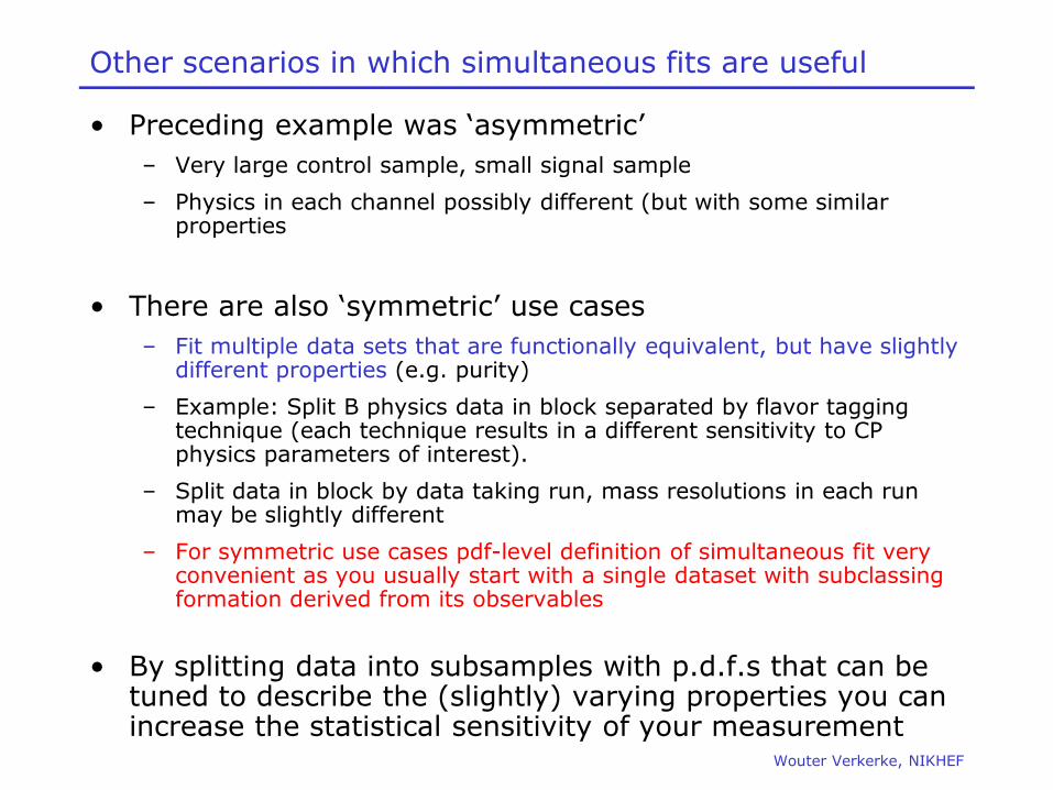
Other scenarios in which simultaneous fits are useful

• Preceding example was ‘asymmetric’ – Very large control sample, small signal sample

– Physics in each channel possibly different (but with some similar properties

• There are also ‘symmetric’ use cases– Fit multiple data sets that are functionally equivalent, but have slightly

different properties (e.g. purity)

– Example: Split B physics data in block separated by flavor tagging – Example: Split B physics data in block separated by flavor tagging technique (each technique results in a different sensitivity to CP physics parameters of interest).

– Split data in block by data taking run, mass resolutions in each run may be slightly different

– For symmetric use cases pdf-level definition of simultaneous fit very convenient as you usually start with a single dataset with subclassingformation derived from its observables

• By splitting data into subsamples with p.d.f.s that can be tuned to describe the (slightly) varying properties you can increase the statistical sensitivity of your measurement


A more empirical approach to simultaneous fits

• Instead of investing a lot of time in developing multi-dimensional models à Split data in many subsamples, fit all subsamples simultaneously to slight variations of ‘master’ p.d.f

• Example: Given dataset D(x,y) where observable of interest is x. – Distribution of x varies slightly with y

– Suppose we’re only interested in the width of the peakwhich is supposed to be invariant under y (unlike mean)

– Slice data in 10 bins of y and simultaneous fit each


– Slice data in 10 bins of y and simultaneous fit each bin with p.d.f that only has different Gaussian mean parameter, but same width


• Fit to sample of preceding page would look like this– Each mean is fitted to expected value (-4.5 + ibin)

Floating Parameter FinalValue +/- Error -------------------- --------------------------

mean_bin1 -4.5302e+00 +/- 1.62e-02mean_bin2 -3.4928e+00 +/- 1.38e-02mean_bin3 -2.4790e+00 +/- 1.35e-02mean_bin4 -1.4174e+00 +/- 9.64e-03mean_bin5 -4.8945e-01 +/- 7.95e-03


– But joint measurement of sigma

– NB: Correlation matrix is mostly diagonal as all mean_binXX parameters are completely uncorrelated!

mean_bin5 -4.8945e-01 +/- 7.95e-03mean_bin6 4.0716e-01 +/- 9.67e-03mean_bin7 1.4733e+00 +/- 1.37e-02mean_bin8 2.4912e+00 +/- 1.44e-02mean_bin9 3.5028e+00 +/- 1.41e-02mean_bin10 4.5474e+00 +/- 1.68e-02

sigma 2.7319e-01 +/- 2.46e-03


• Preceding example was simplistic for illustrational clarity, but more sensible use cases exist– Example: Measurement CP violation in B decay. Analyzing

power of each event is diluted by factor (1-2w) where w is the mistake rate of the flavor tagging algorithm

– Neural net flavor tagging algorithm provides a tagging probability for each event in data. Could use prob(NN) as w, but then we rely on good calibration of NN, don’t want that

– In a simultaneous fit to CPV+Mixing samples, can measure


– In a simultaneous fit to CPV+Mixing samples, can measure average w from the latter. Now not relying on NN calibration, but not exploiting event-by-event variation in analysis power.

– Improved scenario: divide (CPV+mixing) data in 10 or 20 subsets corresponding to bins in prob(NN). Use identical p.d.f but only have separate parameter to express fitted mistag rate w_binXX.

– Simultaneous fit will now exploit difference in analyzing power of events and be insensitive to calibration of flavor tagging NN.

– If calibration of NN was OK fitting mistag rate in each bin of probNN will be average probNN value for that bin


NN predicted power

contr

ol sa

mple

m

easu

red p

ow

er

contr

ol sa

mple

m

easu

red p

ow

er

Perfect NN

OK NN

Better precisionon CPV meas.because moresensitive events in sample


Event with little analyzing power

Event withgreat analyzing

power

NN predicted power

NN predicted power

contr

ol sa

mple

m

easu

red p

ow

er

contr

ol sa

mple

m

easu

red p

ow

er

Lousy NN

In all 3 casesfit not biasedby NN calibration

Worse precisionon CPV meas.because lesssensitive events in sample

Building simultaneous fits from a template

• In the ‘symmetric’ use case the models assigned to each state are very similar in structure – Usually just one parameter name is different

• Easiest way to construct these from a template pdf and a prescription on how to tailor the template for each index state

• Use operator SIMCLONE instead of SIMUL

// Template pdf – B0 decay with mixingw.factory("TruthModel::tm(t[-20,20])") ;w.factory("BMixDecay::sig(t,mixState[mixed=-1,unmixed=1],

tagFlav[B0=1,B0bar=-1], tau[1.54,1,2],dm[0.472,0.1,0.8],w[0.1,0,0.5],dw[0],tm)") ;

// Construct index categoryw.factory(“tag[Lep,Kao,NT1,NT2]”) ;

// Construct simultaneous pdf with separate mistag rate for each categoryw.factory(“SIMCLONE::model(sig,$SplitParam({w,dw},tagCat)”) ;

Building simultaneous fits from a template

• Result

RooWorkspace(w) w contents

variables---------(dm,dw,dw_Kao,dw_Lep,dw_NT1,dw_NT2,mixState,t,tagCat,tagFlav,tau,w,w_Kao,w_Lep,w_NT1,w_NT2)

p.d.f.s-------RooBMixDecay::sig[ mistag=w delMistag=dw mixState=mixState tagFlav=tagFlav tau=tau dm=dm t=t ] = 0.2RooBMixDecay::sig[ mistag=w delMistag=dw mixState=mixState tagFlav=tagFlav tau=tau dm=dm t=t ] = 0.2RooSimultaneous::model[ indexCat=tagCat Lep=sig_Lep Kao=sig_Kao NT1=sig_NT1 NT2=sig_NT2 ] = 0.2RooBMixDecay::sig_Kao[ mistag=w_Kao delMistag=dw_Kao ... t=t ] = 0.2RooBMixDecay::sig_Lep[ mistag=w_Lep delMistag=dw_Lep ... t=t ] = 0.2RooBMixDecay::sig_NT1[ mistag=w_NT1 delMistag=dw_NT1 ... t=t ] = 0.2RooBMixDecay::sig_NT2[ mistag=w_NT2 delMistag=dw_NT2 ... t=t ] = 0.2

analytical resolution models----------------------------RooTruthModel::tm[ x=t ] = 1

Working withLikelihood8


Likelihood8• Using discrete variable to classify data• Simultaneous fits on multiple datasets

Fitting and likelihood minimization

• What happens when you do pdf->fitTo(*data)

– 1) Construct object representing –log of (extended) likelihood

– 2) Minimize likelihood w.r.t floating parameters using MINUIT

• Can also do these two steps explicitly by hand

// Construct function object representing –log(L)


RooAbsReal* nll = pdf.createNLL(data) ;

// Minimize nll w.r.t its parametersRooMinuit m(*nll) ;m.migrad() ;m.hesse() ;

Plotting the likelihood

• A likelihood function is a regular RooFit function

• Can e.g. plot is as usual

RooAbsReal* nll = w::model.createNLL(data) ;

RooPlot* frame = w::param.frame() ;nll->plotOn(frame,ShiftToZero()) ;

Constructing a χ2 function

• Along similar lines it is also possible to construct a χ2

function– Only takes binned datasets (class RooDataHist)

– Normalized p.d.f is multiplied by Ndata to obtain χ2

// Construct function object representing –log(L)RooAbsReal* chi2 = pdf.createChi2(data) ;

– MINUIT error definition for χ2 automatically adjusted to 1 (it is 0.5 for likelihoods) as default error level is supplied through virtual method of function base class RooAbsReal


// Minimize nll w.r.t its parametersRooMinuit m(chi2) ;m.migrad() ;m.hesse() ;

Automatic optimizations in the calculation of the likelihood

• Several automatic computational optimizations are applied the calculation of likelihoods inside RooNLLVar– Components that have all constant parameters are pre-calculated

– Dataset variables not used by the PDF are dropped

– PDF normalization integrals are only recalculated when the ranges of their observables or the value of their parameters are changed

– Simultaneous fits: When a parameters changes only parts of the total likelihood that depend on that parameter are recalculated


total likelihood that depend on that parameter are recalculated• Lazy evaluation: calculation only done when intergal value is requested

• Applicability of optimization techniques is re-evaluated for each use– Maximum benefit for each use case

• ‘Typical’ large-scale fits see significant speed increase– Factor of 3x – 10x not uncommon.

Features of class RooMinuit

• Class RooMinuit is an interface to the ROOT implementation of the MINUIT minimization and error analysis package.

• RooMinuit takes care of– Passing value of miminized RooFit function to MINUIT

– Propagated changes in parameters both from RooRealVar to MINUIT and back from MINUIT to RooRealVar, i.e. it keeps the MINUIT and back from MINUIT to RooRealVar, i.e. it keeps the state of RooFit objects synchronous with the MINUIT internal state

– Propagate error analysis information back to RooRealVarparameters objects

– Exposing high-level MINUIT operations to RooFit uses (MIGRAD,HESSE,MINOS) etc…

– Making optional snapshots of complete MINUIT information (e.g. convergence state, full error matrix etc)


Demonstration of RooMinuit use

// Start Minuit session on above nllRooMinuit m(nll) ;

// MIGRAD likelihood minimizationm.migrad() ;

// Run HESSE error analysism.hesse() ;

// Set sx to 3, keep fixed in fit


// Set sx to 3, keep fixed in fit sx.setVal(3) ;sx.setConstant(kTRUE) ;

// MIGRAD likelihood minimizationm.migrad() ;

// Run MINOS error analysism.minos()

// Draw 1,2,3 ‘sigma’ contours in sx,sym.contour(sx,sy) ;

What happens if there are problems in the NLL calculation

• Sometimes the likelihood cannot be evaluated do due an error condition. – PDF Probability is zero, or less than zero at coordinate where

there is a data point ‘infinitely improbable’

– Normalization integral of PDF evaluates to zero

• Most problematic during MINUIT operations. How to handle error condition– All error conditions are gather and reported in consolidated way


– All error conditions are gather and reported in consolidated way by RooMinuit

– Since MINUIT has no interface deal with such situations, RooMinuit passes instead a large value to MINUIT to force it to retreat from the region of parameter space in which the problem occurred

[#0] WARNING:Minization -- RooFitGlue: Minimized function has error status. Returning maximum FCN so far (99876) to force MIGRAD to back out of this region. Error log follows. Parameter values: m=-7.397 RooGaussian::gx[ x=x mean=m sigma=sx ] has 3 errors


• Classic example in B physics: floating the end point of the ARGUS function– Probability density of ARGUS above end point is zero à If end

point is moved to low value in fit you end up with events above end point à Probility is zero à Likelihood is –log(0) = infinity

pdf and data-log(L) vs m0

dropping problematic events-log(L) vs m0

with ‘wall’ (RooFit default)


• Can request more verbose error logging to debug problem– Add PrintEvalError(N) with N>1

[#0] WARNING:Minization -- RooFitGlue: Minimized function has error status. Returning maximum FCN so far (-1e+30) to force MIGRAD to back out of this region. Error log followsParameter values: m=-7.397 RooGaussian::gx[ x=x mean=m sigma=sx ]

getLogVal() top-level p.d.f evaluates to zero or negative number@ x=x=9.09989, mean=m=-7.39713, sigma=sx=0.1

getLogVal() top-level p.d.f evaluates to zero or negative number




Working with profile likelihood

• A profile likelihood ratio

can be represent by a regular RooFit function(albeit an expensive one to evaluate)

)ˆ,ˆ()ˆ̂,(

)(qpLqpL

p =λ

RooAbsReal* ll = model.createNLL(data,NumCPU(8)) ;RooAbsReal* pll = ll->createProfile(params) ;

47

Best L for given p

Best L

RooPlot* frame = w::frac.frame() ;nll->plotOn(frame,ShiftToZero()) ;pll->plotOn(frame,LineColor(kRed)) ;

Dealing with nuisance parameters in Likelihood ratio intervals

•Likelihood Ratio

•Profile Likelihood Ratio


•Profile Likelihood Ratio

•Minimizes –log(L) for each value of fsigby changing bkg shape params(a 6th order Chebychev Pol)

On the equivalence of profile likelihood and MINOS48

• Demonstration of equivalenceof (RooFit) profile likelihoodand MINOS errors– Macro to make above plots is

34 lines of code (+23 to beautifygraphics appearance)

Constructing joint likelihood

• When you have a simultaneous pdf you can create a joint likelihood from the joint pdf

• Also possible to make likelihood functions of the components first and then add them

RooAbsReal* nllJoint = w::joint.createNLL(dataAB) ;

50

components first and then add them

• Likelihood constructed either way is the same.

• Minimization of joint likelihood == Joint fit

RooAbsReal* nllA = w::A.createNLL(*dataA) ; w.import(nllA) ;RooAbsReal* nllB = w::B.createNLL(*dataB) ; w.import(nllB) ;w.factory(sum::nllJoint(nllA,nllB)) ;

Adding parameter pdfs to the likelihood

• Systematic/external uncertainties can be modeledwith regular RooFit pdf objects.

• To incorporate in likelihood, simply multiply with orig pdf

w.factory(“Gaussian::g(x[-10,10],mean[-10,10],sigma[3])”) ;

w.factory(“PROD::gprime(f,Gaussian(mean,1.15,0.30))”) ;

46

– Any pdf can be supplied, e.g. Gaussian most common, but an also use class RooMultiVarGaussian to introduce a Gaussian uncertainty on multiple parameteres including a correlation

• Advantage of including systematic uncertainties in likelihood: error automatically propagated to error reported by MINUIT

))30.0,15.1,(log(),;(log(),(log µσµσµ GaussxfLdata

i −−−=− ∑

Adding uncertainties to a likelihood

• Example 1 – Width known exactly

• Example 2 – Gaussian uncertainty on width

Using the fit result output

• The fit result class contains the full MINUIT output

• Easy visualization of correlation matrix

• Construct multi-variate Gaussian pdfrepresenting pdf on parameters

fitresult->correlationHist->Draw(“colz”) ;

43

representing pdf on parameters

– Returned pdf represents HESSE parabolic approximation of fit

• Extract correlation, covariance matrix

– Can also retrieve partial matrix (Schur compl.)

RooAbsPdf* paramPdf = fr->createHessePdf(RooArgSet(frac,mean,sigma));

TMatrixDSym cov = fr->covarianceMatrix() ;TMatrixDSym cov = fr->covarianceMatrix(a,b) ;

Another approach to joint fitting

• ‘Asymmetric’ simultaneous fit may spend majority of it CPU time calculating the likelihood of the control sample part– Because control sample have many more events

– Example: joint fit between CPV golden modes and BMixingsamples

• Alternate solution: Make joint fit using likelihood of signal sample and parameterized likelihood of control signal sample and parameterized likelihood of control sample– Assumption: Likelihood can be described by a multi-variate

Gaussian with correlations (i.e. log-likelihood is parabolic)

– Very easy to do in RooFit using RooFitResult->createHessePdf()

– Example on next page

Example of joint fit with parameterized likelihood

// Joint pdf constructionw.factory("SIMUL::model_sim(index[sig,ctl],

sig=model, ctl=model_ctl)") ;

// Joint data constructionRooDataSet simdata("simdata","simdata",w::x,Index(w::index),

Import("sig",*data),Import("ctl",*data_ctl)) ;

// Joint fitRooFitResult* rs = w::model_sim.fitTo(simdata,Save()) ;

Regular joint fit

// Fit to control sample onlyRooFitResult* r = w::model_ctl.fitTo(*data_ctl,Save()) ;RooAbsPdf* ctrlParamPdf = r->createHessePdf(w::model_ctl.getParameters());

// Make pdf of parameters and import in workspacectrlParamPdf->SetName(“ctrlParamPdf”) ;w.import(*ctrlParamPdf) ;w.factory(“PROD::model_sim2(model,ctrlParamPdf)”) ;

// Joint fit with parameterized likelihood for control sampleRooFitResult* rs = w::model_sim2.fitTo(*data,Save()) ;

Joint fit with parameterized L for ctl sample

Intervals & Limits9


Intervals & Limits9• A brief introduction to RooStats

RooStats Project – Overview

• Goals: – Standardize interface for major statistical procedures so that they

can work on an arbitrary RooFit model & dataset and handle many parameters of interest and nuisance parameters.

– Implement most accepted techniques from Frequentist, Bayesian, and Likelihood-based approaches

– Provide utilities to perform combined measurements

• Design:– Essentially all methods start with the basic probability density

function or likelihood function. Building a good model is the hard part. Want to re-use it for multiple methods à Use RooFit to construct models

– Build series of tools that perform statistical procedures on RooFit models


RooStats Project – Structure

• RooFit (data modeling) – Data modeling language (pdfs and likelihoods).

Scales to arbitrary complexity

– Support for efficient integration, toy MC generation

– Workspace • Persistent container for data models

• Completely self-contained (including custom code)

• Complete introspection and access to components

– Workspace factory provides easy scripting language to populate the workspace

• RooStats (limits, interval calculators & utilities) – Profile Likelihood calculator

– Neyman construction (FC)

– Bayesian calculator (BAT & native MCMC)

– Utilities (combinations, construct pdfs corresponding to standard number counting problems)


RooStats Project – Organization

• Joint ATLAS/CMS project

• Core developers– K. Cranmer (ATLAS)

– Gregory Schott (CMS)

– Wouter Verkerke (RooFit)

– Lorenzo Moneta (ROOT)

• Open project, you are welcome to join• Open project, you are welcome to join– Max Baak, Mario Pelliccioni, Alfio Lazzaro contributing now

• Included since ROOT v5.22– Example macros in $ROOTSYS/tutorials/roostats

• Documentation– Code doc. via ROOT

– Esers manual is in development


RooStats Project – Example

• Create a model - Example

RooWorkspace* w = new RooWorkspace(“w”); w->factory(“Poisson::P(obs[150,0,300],

sum::n(s[50,0,120]*ratioSigEff[1.,0,2.],b[100,0,300]*ratioBkgEff[1.,0.,2.]))");

w->factory("PROD::PC(P, Gaussian::sigCon(ratioSigEff,1,0.05), Gaussian::bkgCon(ratioBkgEff,1,0.1))");

)1.0,1,()05.0,1,()|( bsbs rGaussrGaussrbrsxPoisson ⋅⋅⋅+⋅

•Create workspace with above model (using factory)


RooWorkspace(w) w contents

variables---------(b,obs,ratioBkgEff,ratioSigEff,s)

p.d.f.s-------RooProdPdf::PC[ P * sigCon * bkgCon ] = 0.0325554RooPoisson::P[ x=obs mean=n ] = 0.0325554

RooAddition::n[ s * ratioSigEff + b * ratioBkgEff ] = 150RooGaussian::sigCon[ x=ratioSigEff mean=1 sigma=0.05 ] = 1RooGaussian::bkgCon[ x=ratioBkgEff mean=1 sigma=0.1 ] = 1

•Contents of workspace from above operation


• Simple use of modelRooPlot* frame = w::obs.frame(100,200) ;w::PC.plotOn(frame) ;frame->Draw()



• Confidence intervals calculated with model– Profile

likelihood

– FeldmanCousins

ProfileLikelihoodCalculator plc; plc.SetPdf(w::PC); plc.SetData(data); // contains [obs=160]plc.SetParameters(w::s); plc.SetTestSize(.1); ConfInterval* lrint = plc.GetInterval(); // that was easy.

FeldmanCousins fc; fc.SetPdf(w::PC); fc.SetData(data); fc.SetParameters(w::s);

– Bayesian (MCMC)


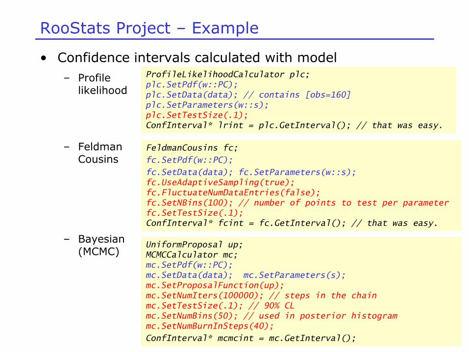
fc.SetData(data); fc.SetParameters(w::s); fc.UseAdaptiveSampling(true); fc.FluctuateNumDataEntries(false); fc.SetNBins(100); // number of points to test per parameter fc.SetTestSize(.1); ConfInterval* fcint = fc.GetInterval(); // that was easy.

UniformProposal up; MCMCCalculator mc; mc.SetPdf(w::PC); mc.SetData(data); mc.SetParameters(s); mc.SetProposalFunction(up); mc.SetNumIters(100000); // steps in the chainmc.SetTestSize(.1); // 90% CL mc.SetNumBins(50); // used in posterior histogram mc.SetNumBurnInSteps(40); ConfInterval* mcmcint = mc.GetInterval();


• Retrieving and visualizing outputdouble fcul = fcint->UpperLimit(w::s);double fcll = fcint->LowerLimit(w::s);



• Some notes on example– Complete working example (with output visualization)

shipped with ROOT distribution ($ROOTSYS/tutorials/roofit/rs101_limitexample.C)

– Interval calculators make no assumptions on internal structure of model. Can feed model of arbitrary complexity to same calculator (computational limitations still apply!)


The end

• RooFit Documentation

• Starting point http://root.cern.ch/drupal/content/roofit– Quick start guide (20 pages) – Includes Workspace & Factory

– Users Manual (140 pages)

• Tutorial macros• Tutorial macros– root.cern.ch à documentation à tutorials à roofit

– There are over 80 macros illustrating many aspects of RooFit functionality

• Help– Post your question on the Stat & Maths tools forum of root.cern.ch

Date post:	18-Apr-2020
Category:	Documents
Upload:	others
View:	5 times
Download:	0 times

Introduction to RooFit - Istituto Nazionale di Fisica...

Documents