Introduction to Sentinel-1Sentinel data use for CAP monitoring and control

Training module at the Vilnius IACS Workshop (28 May 2018)

Guido Lemoine, EC, JRC

Learning objectives of the training

➢ Understanding S1 SAR data use for CAP monitoring and control

➢ Both current OTSC and (focus on) CAP monitoring➢ Linked to “marker” concepts of compliance monitoring

➢ Why is current Sentinel-1 SAR supply different?➢ Why is it a good idea to incorporate S1 SAR, what are

the limitations?➢ What are the practical uptake issues?

Learning objectives of the training (2)

➢ Understanding basics of (Sentinel-1) SAR➢ Introducing physical principles of SAR backscattering➢ Agricultural land use examples

➢ Access and processing needs and tools➢ Demos of core tools in CAP monitoring context➢ Discussion on compute solutions

Structure of the training, timing➢ Overview of (Sentinel-1) SAR characteristics➢ Basic physical principles of S1 SAR backscatter➢ Examples to understand agricultural scenes

➢ Coffee break

➢ Practical S1 data access and processing issues➢ Including scihub, toolbox, Google Earth Engine demos➢ Reflection on processing environment

Introduction to Sentinel-1

Quick review of “Introduction to SAR remote sensing”➢ http://dragon2.esa.int/landtraining2010/pdf/D2L4b_%20LeToan-7Sept10.pdf➢ A shortened version

➢ Other references on SAR [data use]➢ http://www.grss-ieee.org/tutorial-category/sar-tutorials/

➢ Re-hash of important characteristics of Sentinel-1➢ Sentinel-1 SAR Signature use in agriculture

Sentinel cover over Europe

S-1 SAR use in agriculture

➢ Consistent time series of calibrated measurements!➢ Sensitivity to soil surface geometry, soil dielectric

properties, vegetation geometry and properties➢ Translate into sensitivities to soil surface preparation,

soil moisture, freeze/thaw, snow cover, vegetation type and development (structure, water content)

➢ Interpretation is the reverse process: can we identify crop type (and status) from the SAR signature?

S-1 SAR use in agriculture (2)

➢ VV polarized > VH polarized➢ VV polarization is sensitive to crop structure: different

for vertical structured and leaf shape and distribution➢ VH polarization will increase, VV-VH difference will

decrease, with increasing vegetation cover➢ At low vegetation cover, the signal will be a mix of soil

and canopy contributions➢ Be aware of look angle dependency (e.g. ASC/DESC),

esp. for bare soil, row crops (directionality)

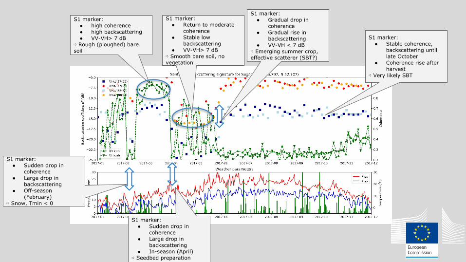
S1 marker:● high coherence● high backscattering● VV-VH> 7 dB

⇨ Rough (ploughed) bare soil

S1 marker:● Sudden drop in

coherence● Large drop in

backscattering● Off-season

(February) ⇨ Snow, Tmin < 0

S1 marker:● Sudden drop in

coherence● Large drop in

backscattering● In-season (April)

⇨ Seedbed preparation

S1 marker:● Return to moderate

coherence● Stable low

backscattering● VV-VH> 7 dB

⇨ Smooth bare soil, no vegetation

S1 marker:● Gradual drop in

coherence● Gradual rise in

backscattering● VV-VH < 7 dB

⇨ Emerging summer crop, effective scatterer (SBT?)

S1 marker:● Stable coherence,

backscattering until late October

● Coherence rise after harvest

⇨ Very likely SBT

S-1 SAR use in agriculture (!)

➢ S-1 backscattering has a solid physical basis➢ S-1 signatures contain information on cropping cycle➢ S-1 data is plentiful available over Europe under full,

free and open license

➢ So, if Sentinel-1 is the best sensor we never used in our life...

➢ … how can we get our hands on these data, how to process, how to analyse?

Sentinel Data Access

➢ Sentinel 1 (and 2) imagery can be accessed via: ➢ https://scihub.esa.int/dhus/

➢ Requires user registration [once]➢ Serves all users, through different interfaces➢ But feeds from one single infrastructure

➢ Combines interactive explore interface (+download)➢ and service end-point for scriptable selection

Sentinel Data Access (2)

➢ Limited to 2 simultaneous downloads per account➢ (but unlimited number of accounts…) ➢ Performance dependent on connection, hub load➢ Shared with > 100,000 users!

➢ GUI search set-up for Sentinel-1, 2 and 3➢ Rather clunky, but OK for occasional selection➢ Beware of regular downtimes (scheduled and not)➢ Archive is still full, but will eventually be “rolling”!

➢ Non-time critical target (NTC) is < 24 hours after acquisition (green line)

➢ Delays beyond NTC are due to:

○ Problems at the PDGS○ Problems at the hub

➢ User only experiences overall delay

➢ Add download timing to get ETA

➢ With current hub congestion, download timing highly variable

Sentinel Data Access (3)

➢ Scriptable access based on OData and OpenSearch➢ Very well documented, with scripts:

○ https://scihub.esa.int/userguide/5APIsAndBatchScripting

➢ Metadata harvesting for preparation of batch downloads

➢ As crontab with python XML-parser + bash➢ Spatial data base (PostgreSQL/Postgis) for

organisation-wide access

Sentinel Data Access (4)

➢ Alternative access:○ Sentinel-hub.com (Sinergise/AWS)○ EODIAS.eu (and other DIAS instances > 20 June)!○ National collaborative ground segment (e.g. PEPS)○ Alaska SAR facility○ Google Earth Engine○ others?

➢ Registration usually required, may be fee-based➢ But, all depend on ingestion in ESA data hub➢ Downloads may be lots faster, though

Sentinel-1 characteristics

➢ C-band SAR, like ERS-{1|2}, ENVISAT, RADARSAT➢ 185 km swath, IW mode at 10 m resolution (land)➢ 12-day revisit per sensor, 6 days combined (S1A + S1B)➢ Combinations with DESCENDING (morning) and

ASCENDING (late afternoon) modes possible➢ Over Europe dual polarization (VV/VH) is default over

land

Sentinel-1 characteristics (2)

➢ Ground-Range Detected (GRD) product contains backscattering intensity (VV + VH) in SAR geometry

➢ i.e. data is ordered in azimuth and range samples. ➢ Each GRD image is ~ 1.6 GB per dual pol scene

➢ Single Look Complex (SLC) product contains backscattering intensity + phase (VV+VH) in SAR geometry

➢ Required for interferometry (e.g. coherence)➢ Each SLC image is ~ 6 GB per dual pol scene

Essential steps in S1 processing

To create “GIS-ready” imagery (recommended order):➢ (Orbit file refinement and Thermal noise removal)➢ Calibration: convert digital numbers to backscattering

coefficients ( 0)➢ Terrain correction: geocode with SRTM DEM (1 or 3

sec), required to convert to projected imagery➢ Results in 10 m pixel spacing

Optional steps in S1 processing

To create “special purpose” imagery:➢ Multi-look: resampling to reduce speckle (but lower

resolution: 20 m or 30 m)➢ Terrain flattening: normalize effects of terrain slope,

useful in (moderately) hilly terrain➢ Speckle filtering: further reduce speckle (e.g.

Refined-Lee)

Introduction to the S1 toolbox

Open source software tool to process Sentinel data➢ http://step.esa.int/main/download/

➢ STEP covers other sensors as well➢ Implemented in Java, cross-platform➢ S1TBX provides functions needed to process SAR data➢ Bundled in SNAP, currently in version 6.0, with

frequent upgrades➢ Has elaborate interface with lots of generic tools as

well

Introduction to the S1 toolbox (2)➢ Can be run interactively and as a batch tool (gpt)➢ Workflow can be defined as a graph (XML)➢ With parameter substitution on command line

➢ Post-processing of SAR is a requirement (SLC or GRD)!

➢ If coherence is required, use SLC!

➢ Linked with scripted download to create GIS-ready SAR imagery “hands free”

Introduction to Google Earth Engine

➢ Google Earth Engine created in 2010➢ Developer platform to demonstrate large scale

distributed computing with co-located massive EO data sets

➢ Free for [scientific] developers➢ Hosting “free, open and redistributable” data sets➢ All MODIS, Landsat, US data sets (e.g. SRTM, NAIP)➢ Sentinel data

GEE client APIs

➢ User defines workflow to select, process and render➢ Workflow can be applied to data in GEE catalogues➢ But also to uploaded [private|shared] user data➢ Rich set of image and feature processing methods➢ Rendering: producing the result of the defined

workflow, e.g. on screen, export to file, client-side evaluation

➢ Workflow can be shared as scripts (not downloads!)➢ JavaScript and python APIs

GEE resources

➢ You need to register for GEE, with a Google Account➢ All GEE documentation online, no books [yet]➢ Entry point: the User guide

https://sites.google.com/site/earthengineapidocs/➢ Full introduction, with basic and advanced code

examples, thematic tutorials, references

➢ Think of GEE as the DIAS we would like to have

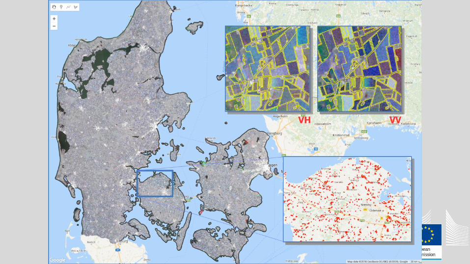
2 exercises using S1 in GEEBasic access and display of Sentinel-1 data

Country mosaic of weekly averaged Sentinel-1 composite

(Requires a Google Earth Engine account!)

Machine learning with S1

➢ Annual declarations form a labelled feature set➢ Can be uploaded to GEE, to extract parcel averages (=

reduction), e.g. from our weekly composites➢ Structured data vectors for machine learning

➢ Many ML frameworks exists, most open source.➢ We use tensorflow➢ On this machine...

Machine learning with S1 (2)

➢ All NL BRP2017 (770 K features, open access Juli 2017)➢ (but also demonstrated with DK2017, BE-VL2017)➢ We select the category “Bouwland” (250K features)➢ For 8 major crops (by area %) and > 0.30 ha (175 K)

➢ Split in 5 sets of 20% training, 80% test samples.➢ Run through tensorflow to identify “outliers”➢ Less than 1 hour runtime.

GRA MAI POT WWH SBT ONI SBA FLO

GRA 0.0 0.0 0.0 0.0 0.0 0.0 0.0 0.0

MAI 0.0 65260.0 374.0 135.0 55.0 52.0 74.0 95.0

POT 0.0 362.0 26126.0 41.0 77.0 25.0 12.0 75.0

WWH 0.0 142.0 37.0 15492.0 7.0 25.0 125.0 12.0

SBT 0.0 134.0 818.0 11.0 12502.0 38.0 3.0 67.0

ONI 0.0 360.0 86.0 148.0 65.0 4439.0 136.0 67.0

SBA 0.0 430.0 23.0 316.0 6.0 54.0 3974.0 21.0

FLO 0.0 203.0 131.0 94.0 331.0 7.0 19.0 2807.0

Overall Accuracy: 96.1

(or 3.9% of parcels are found to have a different than declared label)

Typical result for 1 train/test run

Compute considerations

➢ Data volume estimate for medium size EU state ➢ 4 DESCENDING + 4 ASCENDING passes➢ 2 adjacent frames per orbit➢ i.e. 16 frames per 6 days (~ 1000 frames/year)➢ 1.6 TB (GRD) or 6.4 TB (SLC) per year

➢ Data streams in at an average of 3 frames/day

Compute considerations (2)

➢ Download: 0.5 hr (GRD), 2.0 hr (SLC)➢ Processing with s1tbx: 0.5 hr (GRD), 1.5 hr (SLC)➢ Extraction for 500 K features: 2 hrs➢ Machine learning run: 1 hr

➢ All processing steps can be [parallel] batch procedures➢ Not impossible to handle workload stand-alone➢ Spoilers: scihub delays, internet connectivity and

scihub congestion, fail rates, etc.

Wrap up

➢ We can tweak S1 signatures for the purpose of CAP monitoring

➢ Processing and analysis have a high degree of commonality/shareability/harmonizability

➢ Tools are available, as open source➢ Both cloud and stand-alone option➢ Choice depends on strategy/price/data security, etc.

Wrap up (2)

➢ This seminar is a “teaser”➢ Key message 1: Sentinel-1 is an essential instrument

for CAP monitoring and control➢ Key message 2: Sentinel-1 provides a number of

essential markers on cropping practices➢ Key message 3: processing and analytics of Sentinel-1

is not very different from other sensors➢ Key message 4: Sentinel-1 is ubiquitous, always on,

you don’t want to miss what it can see �

Wrap up (3)

➢ Slides and GEE example code will be made available➢ Additional code, recipes on request (e.g. batch

downloading, s1tbx processing)➢ If you want to see more, contact me during the

workshop➢ Let us know your plans, hesitations, issues!