Introduction to SINDA - Aertia · Introduction to SINDA V4.7 Rev. 0 10/20/04 Page 1 of 25...

Introduction to SINDA V4.7 Rev. 0 10/20/04 Page 1 of 25

Introduction to SINDA

SINDA/FLUINT is a comprehensive software package used by over 400 sites in the aero-space, energy, electronics, automotive, aircraft, HVAC, and petrochemical industries fordesign, simulation, and optimization of systems involving heat transfer and fluid flow. It isthe NASA-standard analyzer for thermal control systems.

This document introduces SINDA, the thermal (conduction/radiation) network capabilities.SINDA represents only part of the complete SINDA/FLUINT package. The fluid networkcapabilities (FLUINT), the graphical user interface (C&R SinapsPlus®), and an additionalplotting package (EZ-XY®) are introduced in separately available documents. Also availableis a CAD-based geometric pre- and post-processor, Thermal Desktop®, with an optional ther-mal radiation analyzer, RadCAD®, and an optional fluid flow analyzer, FloCAD®. Thesetools prepare network information such as conductances, capacitances, convection links,form factors, radiation interchange conductances, and orbital fluxes for SINDA/FLUINTbased on a geometric model, perhaps imported from CAD or structural FEM sources.

What is SINDA?Although classified by some as a finite difference code (versus a finite element code) or as alumped-parameter code, SINDA is actually neither: it is an equation solver. Given appropri-ate inputs, SINDA can produce answers that are the same as those produced by codes thatare based solely on finite elements or finite differences. Most SINDA models are much morefree-form than such codes allow, enabling the creativity and experience of the thermal ana-lyst to be exploited without having to resort to writing specialized, single-use computer pro-grams.

SINDA is a network-style (resistor-capacitor circuit analogy) thermal simulator. The userposes a heat transfer problem by creating an arbitrary network of temperature points(nodes) connected by heat flow paths (conductors). Inputs may be defined indirectly as alge-braic functions, making the code a cross between a spreadsheet and a thermal network ana-lyzer which makes parametric analyses easy to perform. The analyst also defines anarbitrarily complicated solution sequence (perhaps providing auxiliary Fortran-style logic),and chooses the desired output frequencies and formats. Also available are modules for per-forming design optimization, and for automatically adjusting a model to fit test data.

Unconstrained by Geometry

Unlike most structural-oriented finite element codes that feature thermal calculations,SINDA is not geometry-based. Without a tool such as C&R’s Thermal Desktop® (see below),this lack of geometry may make stand-alone SINDA more cumbersome to use than geome-try-based codes for problems with clearly defined, simple geometry. In most cases, however,actual design geometries are much more complex than need to be represented for heat trans-fer solutions, rendering system-level analyses intractable. Geometry-based structuralmeshes and CAD geometry often produce unnecessarily large and inappropriately detailedthermal models that are not only slow to solve but can obscure results.

The situation is analogous to the classic tale of Archimedes’ attempt to calculate the volumeof the king’s ornate crown by piecing together formulae for cones, spheres, etc. (He discov-


ered, of course, that the total volume could be measured as the volume of water displacedwhen the crown was submerged.) If Archimedes had been a thermal engineer he might onlybe concerned with the crown’s total mass and surface area, its interface to the environment,etc. A geometry-based description might have hindered rather than assisted any thermalmodel development.

The lack of geometry makes SINDA more flexible, and more appropriate for undefined orchanging designs, high-level modeling (e.g, entire vehicle), etc. Because of this flexibility andits specialization for heat transfer and fluid flow problems, most analysts use SINDA evenwhen geometry-based codes are available. Often, they employ such codes as pre- and post-processors to SINDA where appropriate.

Empowered by Geometry

Just because a code can solve for temperatures does not make it a thermal analysis tool. Asnoted above, geometry can be constraining and even cumbersome unless an approach consis-tent with the goals and requirements of thermal modeling is applied. Because few such toolsexist, the result has been that thermal calculations, often heavily dependent on nonlineari-ties such as radiation and convection, are rarely performed concurrently with disciplinesrelying on CAD geometry and FEM-based structural models.

C&R’s Thermal Desktop® has been designed specifically to enable a thermal engineer toexploit the existence of CAD-based geometry and to work concurrently with FEM-basedstructural engineers, without having to use their inappropriate models and methods. Ther-mal Desktop allows thermal engineers to work with familiar high-level geometric entities(cones, spheres, panels, etc.) using any combination of finite difference or element tech-niques and exploiting the existence of geometric descriptions and structural models, withoutbeing constrained by the same.

Thermal Desktop is described separately. If you deal with geometric models, radiation (pro-vided by RadCAD®, a module of Thermal Desktop), CAD drawings, and/or require tools to beconcurrent with structural engineering, please refer to that documentation. The remainderof this document deals with stand-alone SINDA, as applied to higher-level modeling tasksnot requiring a geometric description.

Nodes

Nodes represent a point at which energy is conserved. Each node has a single characteristictemperature “T.” Nodes may represent the temperature of a finite volume of material. Theymay be used more abstractly to represent boundary conditions, massless interfaces or edges,effective thermal radiation environments, etc.

There are three types of nodes, classified by their capacitance or ability to transiently storeor release thermal energy.

Diffusion nodes have a finite capacitance “C,” usually equal to the product of mass and spe-cific heat (mCp or ρVCp). Diffusion nodes may represent a finite cell within a meshed vol-ume, or may represent a higher level component such as an electronics chip, a entire card,an entire chassis, a person, a vehicle, etc.

Boundary nodes have an infinite capacitance, and hence usually represent sources or sinks,large masses, or ideally controlled temperature zones.


Arithmetic nodes have zero capacitance: energy flowing into an arithmetic node must bal-ance the energy flowing out at all times. Arithmetic nodes may be used to represent edges,interfaces, negligibly small masses (e.g., radiation shields or foils), and any other tempera-ture to which no mass can or should be assigned.*

Analysts may apply a source or sink of power “Q” to arithmetic and diffusion nodes.

The heat source applied to nodes may vary with time or temperature, and the capacitancemay vary with temperature (e.g., in accordance with material properties). As with any varia-tion in SINDA, these dependencies may be defined by polynomials, table look-ups, or byarbitrarily complex user-defined calculations, spreadsheet interrelationships, and logicalmanipulations. Once defined, material properties, event profiles, etc. can be stored by theuser for reuse in other models.

Conductors

Conductors describe the means by which heat flows from one node to another. Each conduc-tor has a single characteristic conductance “G” (inverse of resistance). Conductors representenergy paths via solid conduction, contact conduction, convection, advection, radiation, etc.

There are two types of conductors.

Linear conductors transport heat in direct proportion to the difference in nodal tempera-tures: Q1-2 = G(T1 - T2), where Q1-2 is the heat flowing from node 1 to node 2 through a con-ductor of value G, T1 is the current temperature of node 1 and T2 is the current temperatureof node 2. Usually, linear conductors represent solid conduction, with G calculated as theproduct of the material conductivity and the internodal cross-sectional area, divided by thedistance between node centers (G = kA/∆x). More complex linear conductors can arise asneeded to represent finite element models, in which case the G is calculated by softwaresuch as C&R’s Thermal Desktop®. Linear conductors may also represent a convection or con-tact conductance times an area (G = hA), among other forms.

Radiation conductors transport heat according to the difference in the fourth power of abso-lute temperature: Q1-2 = G(T1

4 - T24). They are used almost exclusively for radiation heat

transfer, with G = σε1F1-2A1, for example, where σ is the Stefan-Boltzmann constant, ε1 isthe emissivity of node 1, A1 is the area of node 1, and F1-2 is the form factor from node 1 tonode 2. SINDA assumes that radiation conductances are provided by the user: it has no facil-ities for calculating form factors, etc. Geometry-based programs such as C&R’s RadCAD®

(part of the Thermal Desktop) are available that calculate radiation heat transfer conduc-tances and absorbed radiation fluxes specifically for use as inputs to SINDA.

Usage Overview

SINDA is user-extensible, providing the analyst with complete control over inputs, outputs,and solution procedures. SINDA assumes very little about the problem at hand or whichdetails are important to you as the analyst. To use SINDA correctly, you must have ques-tions you want answered, and you must pose them in a way SINDA can comprehend. Thereare no cook-book methods available: the experience and knowledge of the engineer is a vitalingredient in both arriving at a suitable model and an efficient solution approach. While thisstrategy may frustrate the casual user who is looking for an easy “joystick” approach, it

* SINDA divides the world into the finite, the infinite, and the negligible. Engineering judgement must be used to decide which masses and time constants are important, and which can be neglected in order to answer the question at hand.


delights the thermal engineering professional who understands that real thermal problemsrarely lend themselves to such simplistic treatment or to hard-wired assumptions.

The inputs to the program may include:

1. network description: a set of nodes and conductors describing the device or system

2. associated support data if needed: material properties, event profiles such as fluxesversus time, etc. SINDA offers a spreadsheet-like feature for defining key parame-ters (e.g., dimensions, properties) in a central “control panel” such that the remain-der of the inputs can be defined indirectly on the basis of these parameters. Thisspreadsheet feature not only facilitates model building and upkeep, it also enablesparametric analysis, optimization, data correlation, goal seeking, etc.

3. solution sequence: operations to be applied such as a steady-state for initial condi-tions, a parametric series of transient integrations all starting with those initial con-ditions, etc.

4. output operations: including the amount, type, and frequency of outputs

5. control parameters to define or customize units, physical constants, solution accu-racy, etc.

6. supplementary logic, such as convection correlations, or simulation of electronic con-trollers, user-defined devices, etc.

Outputs may be user-defined, but generally include temperatures and heat rates.

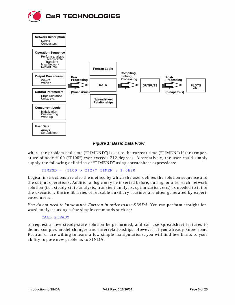
In its traditional form, SINDA is a batch-style code that accepts an ASCII input file andreturns binary and ASCII results files. A Fortran compiler is necessary since each executionof SINDA builds and executes a custom program, as shown in Figure 1.

While SINDA still may be employed in the traditional manner, a graphical user interface,SinapsPlus®, is also available. SinapsPlus retains the geometry-free nature of SINDA: userssketch thermal networks on the screen, launch a run and can even monitor and control itinteractively, and can postprocess (color, plot, etc.) results using such sketches. Users new toSINDA/FLUINT are strongly encouraged to use either SinapsPlus or the Thermal Desktop®

to avoid having to learn the traditional ASCII input file formats. An introduction toSinapsPlus is available separately.

User Logic

In addition to its geometry-independence, the feature that sets SINDA apart from other ana-lyzers is its extensive use of user logic and spreadsheet-like interrelationships to both defineand customize the solution approach. In essence, SINDA uses Fortran as its command lan-guage, although spreadsheet-like interrelationships can alternately be used.

Take the simple example of defining the end of a transient event. Assume that the durationof an event is unknown and is in fact the purpose of the analysis. For example, the analystmight wish to know how long a metal bracket must be placed in a furnace until it achieves acertain temperature, or until a coating melts, etc. With SINDA, a simple line of Fortran-likelogic might be used to detect such an event and terminate the solution:

IF (T100 .GT. 212.0) TIMEND = TIMEN


where the problem end time (“TIMEND”) is set to the current time (“TIMEN”) if the temper-ature of node #100 (“T100”) ever exceeds 212 degrees. Alternatively, the user could simplysupply the following definition of “TIMEND” using spreadsheet expressions:

TIMEND = (T100 > 212)? TIMEN : 1.0E30

Logical instructions are also the method by which the user defines the solution sequence andthe output operations. Additional logic may be inserted before, during, or after each networksolution (i.e., steady state analysis, transient analysis, optimization, etc.) as needed to tailorthe execution. Entire libraries of reusable auxiliary routines are often generated by experi-enced users.

You do not need to know much Fortran in order to use SINDA. You can perform straight-for-ward analyses using a few simple commands such as:

CALL STEADY

to request a new steady-state solution be performed, and can use spreadsheet features todefine complex model changes and interrelationships. However, if you already know someFortran or are willing to learn a few simple manipulations, you will find few limits to yourability to pose new problems to SINDA.

Figure 1: Basic Data Flow

Network DescriptionNodesConductors

Output ProceduresWhat?When?

Concurrent LogicInitialization

Operation SequencePerform analysis

Control ParametersError Tolerance

Steady-StateTransient

Map NetworkRestart, etc. Fortran Logic

DATA

Pre-Compiling,

OUTPUTS PLOTSetc.

Post-

Units, etc.

CustomizingWrap-up

Processing Processing

User DataArraysSpreadsheet

Linking,Processing

(SinapsPlus) (SinapsPlus)

SpreadsheetRelationships


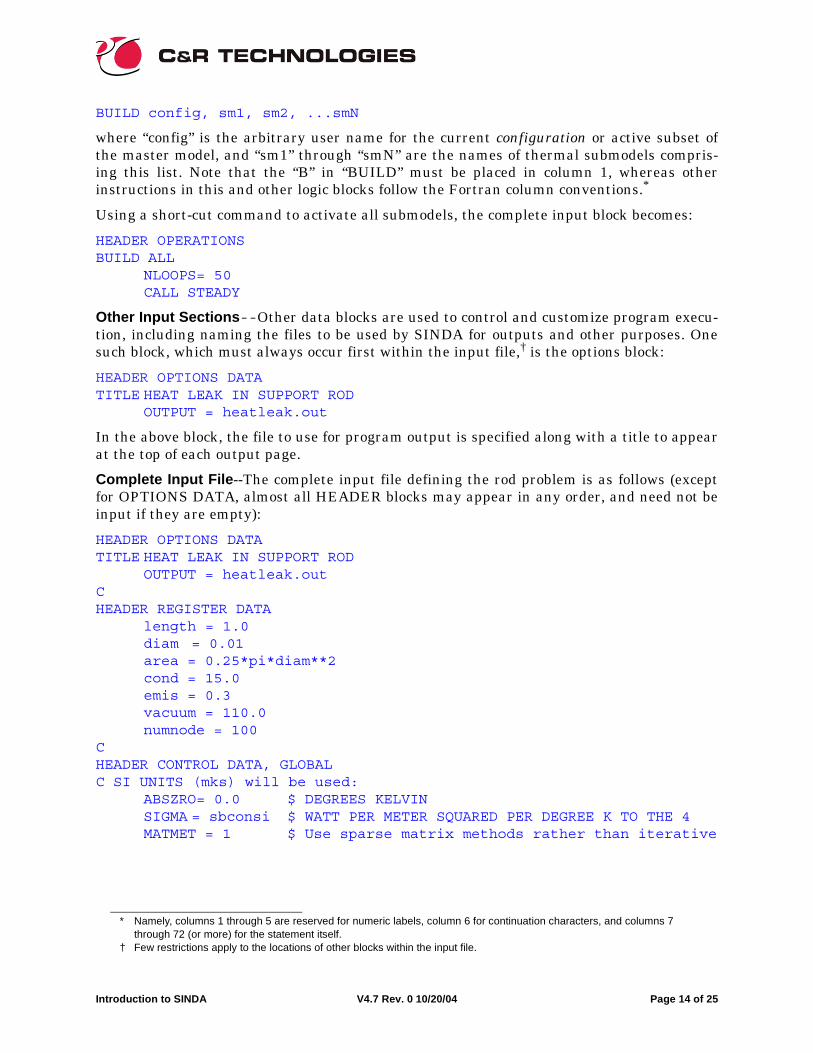
Why SINDA/FLUINT?Because of its popularity and longevity, there are various versions of SINDA and SINDA-like codes available from various sources. Most of those codes represent subsets of SINDA/FLUINT, which uniquely features:

1. Submodels. Networks may be composed of collections of submodels, where each sub-model may be dynamically added or deleted from the solution as needed to modelchanging geometries, materials, boundary conditions, assumptions, etc. Submodels,which are also a great organizational tool, enable SINDA models to be combinedwithout internal numbering or control conflicts. Submodels may consist of nodes,conductors, or both.

2. FLUINT. Complete 1D fluid network solutions may be performed simultaneouslywith or without traditional SINDA networks. From pseudo-steady heat exchangeranalyses to acoustic oscillations in two-phase mixtures, the same generalized andcustomizeable approach that made SINDA successful is also available for internalfluid systems. FLUINT is introduced in a separate document.

3. Built-in Spreadsheet. Models can be defined algebraically with complex expressionsinvolving parentheses, exponentiation, built-in functions, built-in physical constantsand unit conversions, and even user-defined variables called registers. Inputs can bedefined on the basis of other inputs, or even on the basis of as-yet-undefined results(outputs). In addition to improved self-documentation and ease of maintenance,additional analytic power is provided to the user by combining spread-sheet-like fea-tures within a thermal analyzer. Parametric and sensitivity studies can be easilymade without using extensive user logic and without obsolete methods used in olderversions of SINDA.

4. Advanced Design Modules. The Solver is a high-level solution module can be used toprogram SINDA/FLUINT to perform a certain tasks. The Solver can be used to goalseek: to find an input variable given a desired response. It can also be used to per-form multiple-variable design optimization with arbitrarily complex constraints, orto automatically adjust the uncertainties in a model as needed to correlate to testdata (steady state, transient, or a complex mixture of the two), or to seek the worst-case design scenario give a list of variations and uncertainties.

Paralleling the Solver are the statistical design modules, collectively called Reliabil-ity Engineering. These tools allow inputs to be specified not as deterministic valuesbut rather as ranges or probabilistic distributions. The Reliability Engineering mod-ule can then predict the chances that failure criteria will be exceeded. In fact, it canbe combined with the Solver to synthesize a design based on reliability constraints,including perhaps defining what tolerancing is required.

5. SinapsPlus®. A complete graphical user interface that enables visualization ofSINDA/FLUINT inputs and results, and greatly assists in the fine-tuning and docu-mentation of models. It offers many features that have no parallel in SINDA/FLU-INT, including interactive preprocessing and postprocessing, user-definedcomponents, instant re-execute options, and the ability to package SINDA/FLUINTmodels for execution by others. SinapsPlus is introduced in a separate document.

6. Thermal Desktop®, RadCAD®, and FloCAD®. CAD-based and FEM-compatible toolsthat go beyond simple pre- and post-processing to bring true concurrent engineering


capabilities to thermal engineers. Thermal Desktop can be used to launch and post-process SINDA/FLUINT, and Thermal Desktop calculations can be invoked dynami-cally within SINDA/FLUINT logic blocks. The Thermal Desktop suite is introducedin a separate document.

SINDA Sample Problem: BasicThis section develops a simple SINDA model using the traditional ASCII input fileapproach. A demonstration of the same problem using SinapsPlus® is provided in a separatedocument. A template input file is available in the installation set, but this sample will startfrom a blank slate.

Problem Description

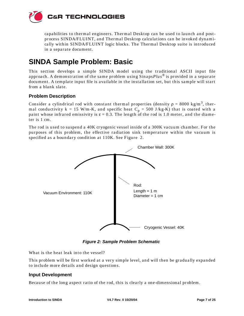
Consider a cylindrical rod with constant thermal properties (density ρ = 8000 kg/m3, ther-mal conductivity k = 15 W/m-K, and specific heat Cp = 500 J/kg-K) that is coated with apaint whose infrared emissivity is ε = 0.3. The length of the rod is 1.0 meter, and the diame-ter is 1 cm.

The rod is used to suspend a 40K cryogenic vessel inside of a 300K vacuum chamber. For thepurposes of this problem, the effective radiation sink temperature within the vacuum isspecified as a boundary condition at 110K. See Figure 2.

What is the heat leak into the vessel?

This problem will be first worked at a very simple level, and will then be gradually expandedto include more details and design questions.

Input Development

Because of the long aspect ratio of the rod, this is clearly a one-dimensional problem.

Rod:Length = 1 mDiameter = 1 cm

Vacuum Environment: 110K

Cryogenic Vessel: 40K

Chamber Wall: 300K

Figure 2: Sample Problem Schematic


Registers--It is useful to start by defining a set of registers containing major problem vari-ables (properties, dimensions, etc.). Changes to these registers in subsequent runs will prop-agate through the input file automatically, facilitating updates. These changes can also bepropagated during a run, facilitating parametric investigations. Registers are the basis formany powerful options in SINDA/FLUINT, so their extensive use is strongly encouraged.

Using arbitrary user-defined names, the basic parameters of the model are defined as:

length = 1.0diam = 0.01area = 0.25*pi*diam**2cond = 15.0emis = 0.3vacuum = 110.0

where “area” is the cross-sectional area of the rod, which will be useful for calculating otherinputs. One register may be defined per line. Note that registers may either be set to con-stants, or to expressions which perhaps use built-in functions (such as sin(x), ln(x), max(x,y)etc.) or built-in constants (such as “pi” in the above expression for “area”), and which perhapscontain references to other registers (such as “diam” in the above expression for “area”).

SINDA input files are subdivided into blocks called Header blocks. The above declarations ofregisters are placed into a section titled HEADER REGISTER DATA. A complete subsectionof the input file is therefore:

HEADER REGISTER DATAlength = 1.0diam = 0.01area = 0.25*pi*diam**2cond = 15.0emis = 0.3vacuum = 110.0

Notice that the “H” in HEADER must be placed in column 1. This is one of the few columnrestrictions in SINDA/FLUINT. Column 1 is reserved for certain top-level commands.

Nodes--The problem has three boundary conditions: the chamber wall, the effective vacuumenvironment, and the vessel wall. Each will be represented by boundary nodes that arelabeled 1000, 2000, and 3000 respectively.

Using a traditional ASCII input file (instead of SinapsPlus® or Thermal Desktop®), thesenodes may be input by specifying a node number (which if negative signals a boundarynode), an initial temperature (which in the case of a boundary node will not change), and aninitial capacitance (which in the case of a boundary node is zero) for each node. This portionof the input file might look like:

-1000, 300.0, 0.0 $ Boundary node for chamber wall-2000, vacuum, 0.0 $ Boundary node for vacuum environment-3000, 40.0, 0.0 $ Boundary node for vessel wall

Note the use of dollar signs (“$”) to denote in-line comments. (A “C” in column 1 makes theentire line a comment.) While hard-wired values were input for the chamber and vessel walltemperature, the temperature of the vacuum environment was chosen to be input paramet-


rically by referring to the register named vacuum, which was defined in a separate section(above).

The problem can be solved entirely by steady-state solutions, since no transient event exists.The rod may therefore be represented by zero capacitance (massless) arithmetic nodes. Thischoice eliminates the need to calculate the capacitances that would be required if diffusionnodes had been chosen. In steady state solutions, diffusion nodes are treated as arithmeticnodes, so their capacitances will therefore be ignored in this case. Thus, there is no need foreither density or specific heat data.

How many such nodes should be used, and how should the rod be discretized? The goal of theanalysis is the prediction of the heat leak into the vessel, and the accuracy of that calculationwill depend on the “length” of the final conductor next to the vessel wall, as shown in Figure3. The gradient in the rod near the vessel is used to calculate the heat flowing into the ves-sel. If the rod is divided into n equal lengths, then the heat flow into the vessel is Q = kA(Tn- T3000)/(L/2n), where A is the cross sectional area of the rod, L is the total length, and Tn isthe temperature of the last (nth) node.

The more nodes that are used to represent the rod, the better the resulting accuracy of theheat leak calculation. In SINDA, the cost of the solution is approximately proportional ton*log(n),* where n is the number of nodes. In other words, a model with 10 nodes might besolved in about one twentieth of the time it takes to solve a model with 100 nodes. Nonethe-less, a 100 node problem represents a relatively small model in SINDA, which can accommo-date tens of thousands of nodes. Therefore, 100 will be chosen as the desired resolution.

The only fail-safe way to find out if enough resolution has been used is to rerun the modelwith a different number of nodes and see if the results change significantly. Most experi-enced analysts quickly develop rules-of-thumb and intuition based on experience. One such

* In many matrix-based finite element solvers, the solution cost grows much faster with model size: about n2.

Figure 3: Discretization Requirement is Governed by Desired Result

Bdy.Node

Arit.Node

Arit.Node

LinearConductor

L/n

L/(2n)

3000

n-1

n

A = πD2/4Gn-3000 = kA/(L/2n)

Qn-3000= Gn-3000(Tn - T3000)

D

L/n


rough rule-of-thumb is that no two adjacent nodes should differ by more than about 3 to 5°C(about 5 to 10°F). Knowing that the range in this model is 300-40=260K, this rule-of-thumbyields a resolution on the order of 50 to 100, so 100 should be a safe bet. (In the correspond-ing SinapsPlus® development of this same model, the error resulting from a 10 node model isrevealed.)

To facilitate changes to this resolution decision, the number of nodes is itself defined as aregister:

HEADER REGISTER DATAlength = 1.0diam = 0.01area = 0.25*pi*diam**2cond = 15.0emis = 0.3vacuum = 110.0numnode = 100

To generate 100 identical nodes, a single SINDA input command may be used that definesthe identifier of the first node, the number of nodes to generate, the increment to use in nam-ing the nodes (enabling sequences such as 5,10,15,20, ... to be generated), the initial temper-ature, and the initial capacitance. For arithmetic nodes, a negative capacitance is used as aninput signal. As will become evident, SINDA frequently uses negative signs as input signals.The generic format of the node GEN statement is as follows:

GEN N#, #N, NINC, T, C

where N# means a node number (the first to be generated), #N means number of nodes,NINC means node number increment, and T and C mean initial temperature and capaci-tance, respectively. If the nodes are numbered sequentially from 1 to 100, the command is asfollows:

GEN 1,numnode,1,100.0,-1.0 $ 100 Arit. nodes representing the rod

The initial temperature of 100.0 is strictly an initial guess that will be quickly overwrittenonce the solution starts. The register name vacuum could have been substituted for “100.0”in the above input line to provide an even more generic initial guess.

All the data describing nodes is placed in a header block called HEADER NODE DATA.Actually, there may be more than one network or submodel in each model, for purposes thatare described later. Therefore, even if there is only one submodel in this sample problem, itmust be given a unique alphanumeric name (just as each node must be given a numericidentifier that is unique within its submodel). Using “ROD” as the submodel name yields thecomplete input block:

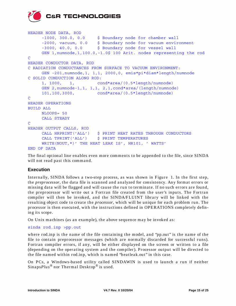
HEADER NODE DATA, ROD

-1000, 300.0, 0.0 $ Boundary node for chamber wall-2000, vacuum, 0.0 $ Boundary node for vacuum environment-3000, 40.0, 0.0 $ Boundary node for vessel wallGEN 1,numnode,1,100.0,-1.0 $ 100 Arit. nodes representing the rod


Conductors--The next step in the modeling process is to identify heat flow paths, which willbe modeled by conductors. In this simple model, there are two types of such paths: axial con-duction along the rod, and radiation exchange between the surface of the rod and the vac-uum environment. Linear conductors will be used to represent solid conduction within therod, and radiation conductors will be used to represent the exchange between the rod andthe vacuum environment.

To generate a single conductor, the simplest command is to provide the name (uniquenumeric identifier) of the conductor, the pair of nodes to which it connects, and the initialconductance. The generic format for conductor input is:

G#, NA#, NB#, G

where G# is the conductor number or identifier, NA# and NB# are the numbers of the nodesto which they connect, and G is the initial conductance.

Linear conductors have positive identifiers, and radiation conductors are signaled with anegative sign:

1020, 10, 20, 5.0 $ linear conductor #1020 from node 10 to 20-333, 1, 2, 5.0E-10 $ radiation conductor #333

The units of the linear and radiation conductances will not be the same, since linear conduc-tances have units of power per degree, and radiation conductances have units of power perdegree4. As long as the user provides nodal sources and capacitances that obey a consistentunit system, SINDA does not enforce a unit convention. In order to employ radiation conduc-tances, however, the value of absolute zero temperature (“ABSZRO”) in the current unit sys-tem must be defined. Also, it is convenient to define the Stefan-Boltzmann constant once as“SIGMA” rather than repeating it in every radiation conductor’s conductance. Such model-level numbers are placed in a data block called HEADER CONTROL DATA, which appliesto all submodels if the special name “GLOBAL” is used. For the current problem:

HEADER CONTROL DATA, GLOBALC SI UNITS (mks) will be used:

ABSZRO = 0.0 $ DEGREES KELVINSIGMA = sbconsi $ WATT PER METER SQUARED PER DEGREE K TO THE 4MATMET = 1 $ Use sparse matrix methods rather than iterative

Note that “sbconsi” is a built-in value (as is “pi”) of the Stefan-Boltzmann constant in SIunits, corresponding to 5.67E-8 W/m2K4. The “MATMET = 1” directive elects the direct(sparse matrix) solution rather than the default iterative method. In SINDA/FLUINT, thesolution method can be tailored submodel by submodel, for truly customized solutionschemes.

Returning to the creation of the conductors, a single GEN statement can be used to create allof the radiation conductances. The format for the conductor GEN option is:

GEN G#,#G,GINC, NA#,NAINC, NB#,NBINC, G

Hence the resulting SINDA input statement, using built-in constants and user-defined reg-isters, is:

C Radiation conductors from rod surface to vacuumGEN -201,numnode, 1, 1, 1, 2000,0, emis*pi*diam*length/numnode


where the 100 conductors will be numbered sequentially from 201 to 300. In other words,“201,numnode,1” in the above statement means to create 100 (=numnode) conductors start-ing with number 201 and incrementing the identifiers by 1. The statement also details thenodes to which the generated conductors will connect: node 1 through 100 on one end, andnode 2000 on the other end. “1,1” defines the first node: number 1 with an increment of 1.Similarly, “2000,0” means to connect all conductors to node number 2000 on the other end(since the increment is zero). The above GEN statement is equivalent to the following indi-vidually input conductors:

-201, 1, 2000, emis*pi*diam*length/numnode-202, 2, 2000, emis*pi*diam*length/numnode-203, 3, 2000, emis*pi*diam*length/numnode...{et cetera}...-299, 99,2000, emis*pi*diam*length/numnode-300,100,2000, emis*pi*diam*length/numnode

In this case, the GEN statement generates a “fan” of conductors since they all connect to acommon node (#2000) on one end. (This designation would become evident if the networkwere drawn in SinapsPlus®.)

Note the arithmetic operations for the last entry, which collectively represent an expressionfor the conductance. The formula being applied is “επD∆L”, where the length of each node is“length/numnode”.

For the linear conductors that will be used to represent axial conduction, a single GEN state-ment cannot be used since all such conductors are not equal. As is evident in Figure 3, thefirst and last conductors are half-length, and therefore will have twice the conductance ofthe rest. Furthermore, these end conductors do not connect to nodes whose names lendthemselves to a single incremental naming scheme. Statements generating these conduc-tors, numbered 1 through 101, would be:

1, 1000, 1, cond*area/(0.5*length/numnode)GEN 2, numnode-1, 1, 1, 1, 2, 1, cond*area/(length/numnode)101,100,3000, cond*area/(0.5*length/numnode)

where the expression G in each of the above statements represents the formula: kπD2/(4∆X),exploiting the fact that “area” has been predefined as πD2/4.

Although not a requirement, it is convenient to place all of the conductors in the same sub-model as the nodes, namely “ROD.” The final conductor data block therefore becomes:

HEADER CONDUCTOR DATA, RODC RADIATION CONDUCTANCES FROM SURFACE TO VACUUM ENVIRONMENT:

GEN -201,numnode,1, 1,1, 2000,0, emis*pi*diam*length/numnodeC SOLID CONDUCTION ALONG ROD:

1, 1000, 1, cond*area/(0.5*length/numnode)GEN 2,numnode-1,1, 1,1, 2,1,cond*area/(length/numnode)101,100,3000, cond*area/(0.5*length/numnode)

Output Specifications--All of the previously described inputs are data blocks since theyspecify network data rather than execution instructions. Unlike previously described inputs,the desired outputs are specified by a logic block. Logic blocks are pseudo-Fortran listingsthat are converted into real Fortran by SINDA, and then compiled and executed. To specify


the desired outputs, the user supplies the output operations to be performed by the code atpredefined intervals, using canned routines and/or user-supplied output instructions:

HEADER OUTPUT CALLS, RODCALL HRPRINT(’ALL’) $ PRINT HEAT RATE THROUGH CONDUCTORSCALL TPRINT(’ALL’) $ PRINT TEMPERATURESWRITE(NOUT,*)’ THE HEAT LEAK IS’, -HR101, ’ WATTS’

The routine “HRPRINT” prints out the heat rate through the conductors for the specifiedsubmodel (‘ALL’ refers to all active submodels). TPRINT functions analogously, printing thenodal “T” or temperature.

In the above block, “HR101” means the heat rate through conductor 101. This variable istranslated by SINDA into a reference to a cell in a Fortran array. While the details of thetranslation are usually not important, it is necessary to know that such translations occur,and that they can be customized and controlled. By the way, “G101” means the conductanceof conductor 101 while “T3000” and “C3000” mean the temperature and capacitance of node3000,

By default, OUTPUT CALLS is executed before and after each steady-state solution,although the user can customize the calling frequency if desired.

Solution Sequence--Like OUTPUT CALLS, the entire solution sequence is specified as alogic block, meaning that the user has complete control over program execution from start tofinish. The solution sequence is specified in a header block called HEADER OPERATIONS.Instructions placed in this block will become the main driver for the run. It will be turnedinto a once-through subroutine, meaning that once the operations contained in that blockhave been executed, the program will stop.

In this particular sample problem, a single steady-state run is needed. Such solutions arerequested by calling single routines such as:

CALL STEADY

The user may select the maximum number of iterations that each steady-state call mayattempt before either convergence is achieved or the program gives up. (The default is 1000.)Each iteration represents a single pass through the solution equations, with each nodal tem-perature being updated once, either iteratively or directly. Like ABSZRO and SIGMA, themaximum number of iterations is a control constant named NLOOPS. Generally, NLOOPSshould be set to the maximum size the user can afford: a number that is normally estimatedbased on prior experience and knowledge of each model. Generally, the larger the model, themore iterations will be required to solve it. For this current model, 50 is chosen as a limitsince it uses direct (sparse matrix) methods:

NLOOPS = 50

This statement may be placed in logic block HEADER OPERATIONS prior to the call toSTEADY, or it may be placed in the data block HEADER CONTROL DATA, GLOBAL,where initializations may be made. This data block just happens to have a format that looksa lot like a logic block.

Since SINDA/FLUINT can apply multiple submodels to any problem, the list of submodelsthat will participate in the next solution must be defined. This list is declared by a BUILDstatement of the format:


BUILD config, sm1, sm2, ...smN

where “config” is the arbitrary user name for the current configuration or active subset ofthe master model, and “sm1” through “smN” are the names of thermal submodels compris-ing this list. Note that the “B” in “BUILD” must be placed in column 1, whereas otherinstructions in this and other logic blocks follow the Fortran column conventions.*

Using a short-cut command to activate all submodels, the complete input block becomes:

HEADER OPERATIONSBUILD ALL

NLOOPS= 50CALL STEADY

Other Input Sections--Other data blocks are used to control and customize program execu-tion, including naming the files to be used by SINDA for outputs and other purposes. Onesuch block, which must always occur first within the input file,† is the options block:

HEADER OPTIONS DATATITLE HEAT LEAK IN SUPPORT ROD

OUTPUT = heatleak.out

In the above block, the file to use for program output is specified along with a title to appearat the top of each output page.

Complete Input File--The complete input file defining the rod problem is as follows (exceptfor OPTIONS DATA, almost all HEADER blocks may appear in any order, and need not beinput if they are empty):

HEADER OPTIONS DATATITLE HEAT LEAK IN SUPPORT ROD

OUTPUT = heatleak.outCHEADER REGISTER DATA

length = 1.0diam = 0.01area = 0.25*pi*diam**2cond = 15.0emis = 0.3vacuum = 110.0numnode = 100

CHEADER CONTROL DATA, GLOBALC SI UNITS (mks) will be used:

ABSZRO= 0.0 $ DEGREES KELVINSIGMA = sbconsi $ WATT PER METER SQUARED PER DEGREE K TO THE 4MATMET = 1 $ Use sparse matrix methods rather than iterative

* Namely, columns 1 through 5 are reserved for numeric labels, column 6 for continuation characters, and columns 7 through 72 (or more) for the statement itself.

† Few restrictions apply to the locations of other blocks within the input file.


HEADER NODE DATA, ROD-1000, 300.0, 0.0 $ Boundary node for chamber wall-2000, vacuum, 0.0 $ Boundary node for vacuum environment-3000, 40.0, 0.0 $ Boundary node for vessel wallGEN 1,numnode,1,100.0,-1.0$ 100 Arit. nodes representing the rod

CHEADER CONDUCTOR DATA, RODC RADIATION CONDUCTANCES FROM SURFACE TO VACUUM ENVIRONMENT:

GEN -201,numnode,1, 1,1, 2000,0, emis*pi*diam*length/numnodeC SOLID CONDUCTION ALONG ROD:

1, 1000, 1, cond*area/(0.5*length/numnode)GEN 2,numnode-1,1, 1,1, 2,1,cond*area/(length/numnode)101,100,3000, cond*area/(0.5*length/numnode)

CHEADER OPERATIONSBUILD ALL

NLOOPS= 50CALL STEADY

CHEADER OUTPUT CALLS, ROD

CALL HRPRINT(’ALL’) $ PRINT HEAT RATES THROUGH CONDUCTORSCALL TPRINT(’ALL’) $ PRINT TEMPERATURESWRITE(NOUT,*)’ THE HEAT LEAK IS’, HR101, ’ WATTS’

END OF DATA

The final optional line enables even more comments to be appended to the file, since SINDAwill not read past this command.

Execution

Internally, SINDA follows a two-step process, as was shown in Figure 1. In the first step,the preprocessor, the data file is scanned and analyzed for consistency. Any format errors ormissing data will be flagged and will cause the run to terminate. If no such errors are found,the preprocessor will write out a Fortran file created from the user’s inputs. The Fortrancompiler will then be invoked, and the SINDA/FLUINT library will be linked with theresulting object code to create the processor, which will be unique for each problem run. Theprocessor is then executed, with the instructions defined in OPERATIONS completely defin-ing its scope.

On Unix machines (as an example), the above sequence may be invoked as:

sinda rod.inp >pp.out

where rod.inp is the name of the file containing the model, and “pp.out” is the name of thefile to contain preprocessor messages (which are normally discarded for successful runs).Fortran compiler errors, if any, will be either displayed on the screen or written to a file(depending on the operating system and the compiler). Processor output will be directed tothe file named within rod.inp, which is named “heatleak.out” in this case.

On PCs, a Windows-based utility called SINDAWIN is used to launch a run if neitherSinapsPlus® nor Thermal Desktop® is used.


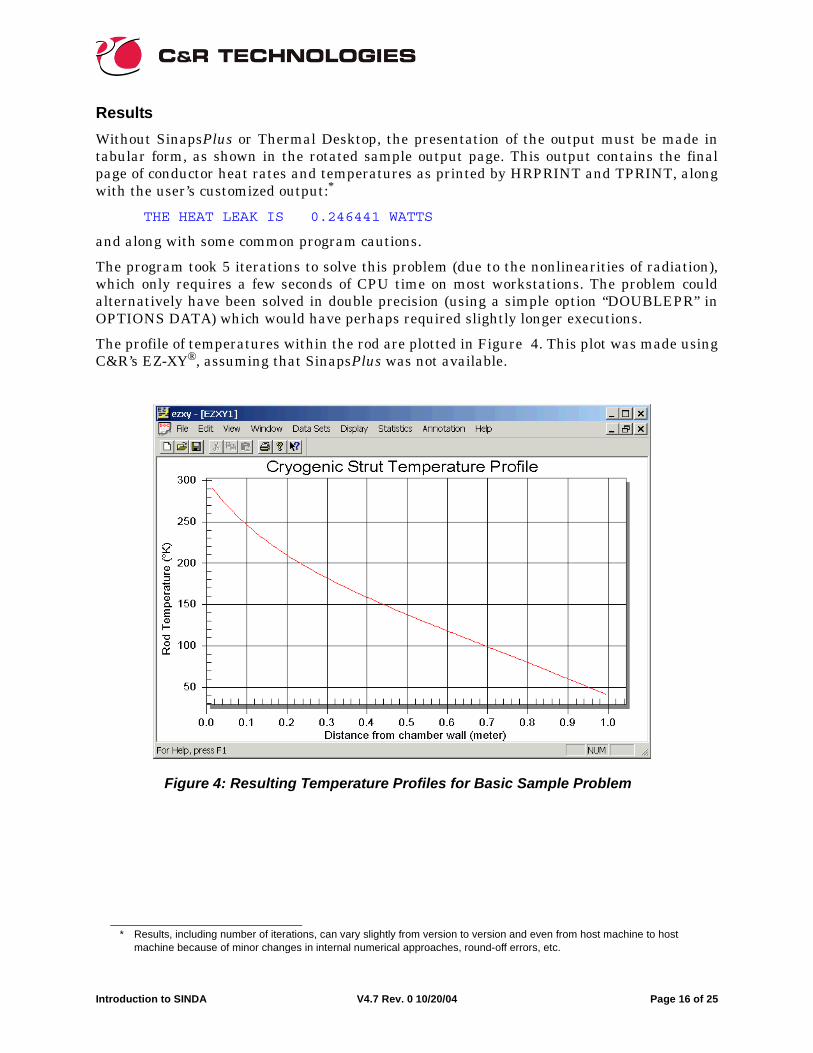
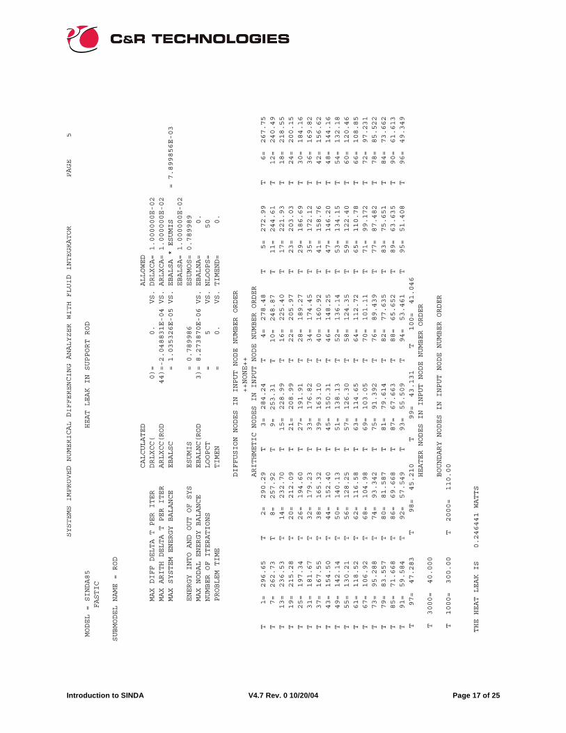
Results

Without SinapsPlus or Thermal Desktop, the presentation of the output must be made intabular form, as shown in the rotated sample output page. This output contains the finalpage of conductor heat rates and temperatures as printed by HRPRINT and TPRINT, alongwith the user’s customized output:*

THE HEAT LEAK IS 0.246441 WATTS

and along with some common program cautions.

The program took 5 iterations to solve this problem (due to the nonlinearities of radiation),which only requires a few seconds of CPU time on most workstations. The problem couldalternatively have been solved in double precision (using a simple option “DOUBLEPR” inOPTIONS DATA) which would have perhaps required slightly longer executions.

The profile of temperatures within the rod are plotted in Figure 4. This plot was made usingC&R’s EZ-XY®, assuming that SinapsPlus was not available.

* Results, including number of iterations, can vary slightly from version to version and even from host machine to host machine because of minor changes in internal numerical approaches, round-off errors, etc.

Figure 4: Resulting Temperature Profiles for Basic Sample Problem


SYSTEMS IMPROVED NUMERICAL DIFFERENCING ANALYZER WITH FLUID INTEGRATOR PAGE 5

MODEL = SINDA85 HEAT LEAK IN SUPPORT ROD

FASTIC

SUBMODEL NAME = ROD

CALCULATED ALLOWED

MAX DIFF DELTA T PER ITER DRLXCC( 0)= 0. VS. DRLXCA= 1.000000E-02

MAX ARITH DELTA T PER ITER ARLXCC(ROD 44)=-2.048831E-04 VS. ARLXCA= 1.000000E-02

MAX SYSTEM ENERGY BALANCE EBALSC = 1.035326E-05 VS. EBALSA * ESUMIS = 7.899856E-03

EBALSA= 1.000000E-02

ENERGY INTO AND OUT OF SYS ESUMIS = 0.789986 ESUMOS= 0.789989

MAX NODAL ENERGY BALANCE EBALNC(ROD 3)= 8.273870E-06 VS. EBALNA= 0.

NUMBER OF ITERATIONS LOOPCT = 5 VS. NLOOPS= 50

PROBLEM TIME TIMEN = 0. VS. TIMEND= 0.

DIFFUSION NODES IN INPUT NODE NUMBER ORDER

++NONE++

ARITHMETIC NODES IN INPUT NODE NUMBER ORDER

T 1= 296.65 T 2= 290.29 T 3= 284.24 T 4= 278.48 T 5= 272.99 T 6= 267.75

T 7= 262.73 T 8= 257.92 T 9= 253.31 T 10= 248.87 T 11= 244.61 T 12= 240.49

T 13= 236.53 T 14= 232.70 T 15= 228.99 T 16= 225.40 T 17= 221.93 T 18= 218.55

T 19= 215.28 T 20= 212.09 T 21= 208.99 T 22= 205.97 T 23= 203.03 T 24= 200.15

T 25= 197.34 T 26= 194.60 T 27= 191.91 T 28= 189.27 T 29= 186.69 T 30= 184.16

T 31= 181.67 T 32= 179.23 T 33= 176.82 T 34= 174.45 T 35= 172.12 T 36= 169.82

T 37= 167.55 T 38= 165.32 T 39= 163.10 T 40= 160.92 T 41= 158.76 T 42= 156.62

T 43= 154.50 T 44= 152.40 T 45= 150.31 T 46= 148.25 T 47= 146.20 T 48= 144.16

T 49= 142.14 T 50= 140.13 T 51= 138.13 T 52= 136.14 T 53= 134.15 T 54= 132.18

T 55= 130.21 T 56= 128.25 T 57= 126.30 T 58= 124.35 T 59= 122.40 T 60= 120.46

T 61= 118.52 T 62= 116.58 T 63= 114.65 T 64= 112.72 T 65= 110.78 T 66= 108.85

T 67= 106.92 T 68= 104.98 T 69= 103.05 T 70= 101.11 T 71= 99.172 T 72= 97.231

T 73= 95.288 T 74= 93.342 T 75= 91.392 T 76= 89.439 T 77= 87.482 T 78= 85.522

T 79= 83.557 T 80= 81.587 T 81= 79.614 T 82= 77.635 T 83= 75.651 T 84= 73.662

T 85= 71.668 T 86= 69.668 T 87= 67.663 T 88= 65.652 T 89= 63.635 T 90= 61.613

T 91= 59.584 T 92= 57.549 T 93= 55.509 T 94= 53.461 T 95= 51.408 T 96= 49.349

T 97= 47.283 T 98= 45.210 T 99= 43.131 T 100= 41.046

HEATER NODES IN INPUT NODE NUMBER ORDER

T 3000= 40.000

BOUNDARY NODES IN INPUT NODE NUMBER ORDER

T 1000= 300.00 T 2000= 110.00

THE HEAT LEAK IS 0.246441 WATTS


SINDA Sample Problem: More DetailsIn this section, the previously defined sample problem will be reworked in increasing detail,illustrating key SINDA features.

Variation 1: Transient Analyses and Simple User Logic

In addition to steady-state analyses, SINDA may be used to predict transient events. A sta-ble second-order implicit integration routine is the standard choice, although others areavailable. Time steps are automatically estimated to control error generation, although likemost other SINDA features, this may be easily modified or overridden by the analyst.

Extending the previous sample, assume that a 100 Watt heater, located on the rod 10cmaway from the vessel, is turned on at time zero. It is desired to know how long such a loadcan be applied before the heat leak into the vessel exceeds 1W. The heat source can beapplied to node 90 using HEADER SOURCE DATA as follows:

HEADER SOURCE DATA,ROD90, 100.0

However, this load would then apply for all times, including the initial condition. To imposethe load only during the transient event, several options exist:

1. Save the initial conditions from a previous run (see “Restarts and Parametric Analy-ses” below)

2. Define a time-varying source, such that a step function is applied at time zero (see“Utilities for Time- and Temperature-dependent Variations” below)

3. Turn the heater on using a simple line of Fortran logic by making the source applieda variable instead of a constant “100.0”

4. Define the source as a time-varying expression

A new register named “power” is used and initialized to 100.0 to facilitate future changes.Along with the definition of specific heat and density, which are needed in this transientanalysis, the new REGISTER block becomes:

HEADER REGISTER DATAlength = 1.0diam = 0.01area = 0.25*pi*diam**2cond = 15.0emis = 0.3vacuum = 110.0numnode = 100spheat = 500.0density = 8000.0power = 100.0

This variable can then be applied as a source to node #90, using a conditional expressionusing the SINDA variable “TIMEN” meaning “time now” (current problem time):


HEADER SOURCE DATA,ROD90, (timen > 0.)? power : 0. $ Use POWER in transients, else

$ zero when time is zero.

The problem end time is unknown, and determining it is in fact the purpose of the analysis.To stop the run at the desired time, the end time (TIMEND) is set to the current time whenthe termination event is detected, otherwise a large value (1000 seconds) is used:

HEADER CONTROL DATA, GLOBAL...TIMEND = (ROD.HR101 >= 1.)? timen : 1000.

The new OPERATIONS block becomes:

HEADER OPERATIONSBUILD ALLDEFMOD ROD $ “ROD” IS THE DEFAULT SUBMODEL

NLOOPS= 50CALL STEADY $ PERFORM A STEADY STATE ANALYSIS.CALL TRANSIENT $ START THE TRANSIENT EVENT

More modifications are needed to the previous model, since the massless arithmetic nodesused in the last problem would react instantaneously to the step increase in heater power,arriving at the final steady-state temperature values instantaneously. Mass must be addedto the model by converting the rod nodes from arithmetic to diffusion:

HEADER NODE DATA, ROD-1000, 300.0, 0.0 $ Boundary node for chamber wall-2000, vacuum, 0.0 $ Boundary node for vacuum environment-3000, 40.0, 0.0 $ Boundary node for vessel wall

C 100 Diffusion nodes representing the rod:GEN 1,numnode,1,100.0, spheat*density*area*(length/numnode)

where the final expression represents the capacitance term: CpρA∆X.

When all of the above modifications are made, the program predicts that it will take 204 sec-onds for the heat leak into the vessel to exceed 1 Watt.

Variation #3, Goal Seeking, shows a more generalized means by which the user can find anykey value (perhaps even an input value) as a function of a desired response.

Variation 2: Restarts and Parametric Analyses

Ordinarily, the initial conditions (temperatures, heat sources, etc.) specified in NODE andCONDUCTOR DATA are progressively updated by whatever operations are specified inOPERATIONS. For example, a call to STEADY resets the nodal temperatures with what-ever results are appropriate for a steady-state solution. A subsequent call to a transientsolution routine (e.g., TRANSIENT) begins wherever STEADY left off. In other words, theresults of the steady-state solution are used as initial conditions for the transient routine.

Of course, the user may elect instead to launch a series of parametric steady-state analyses,perhaps using a Fortran “DO” loop or a prepackaged SINDA option. Each steady-state solu-tion is performed using the results of the previous analysis as a starting point. While thisapproach may be valid for a series of steady-state solutions, it would not be appropriate for aseries of parametric transient solutions that must all start from the same initial conditions.


SINDA provides several utilities that enable the analyst to save “snapshots” of the currentmodel for reuse either later in the same run (“parametric”) or in a future run (“restart”). Inthe above case of multiple transients starting from the same point, the routines SVPARTand RESPAR can be used to respectively capture and restore the initial conditions. As manysuch states or snapshots can be captured as needed. Each stored state is identified by anumeric (integer) key, which may be stored in a Fortran integer variable.

To continue the previous sample problem, what if the design question were to calculate themaximum heater power which can be applied over a 3 minutes period such that the heatleak into the vessel will not exceed 1W. Knowing that it takes over 200 seconds at 100W, aparametric transient analysis can conveniently bracket the question:

HEADER OPERATIONSBUILD ALLDEFMOD ROD $ 'ROD' IS THE DEFAULT SUBMODELC

NLOOPS = 50CALL STEADY $ GENERATE INITIAL CONDITIONSCALL SVPART('T',MTEST) $ SAVE TEMPERATURES IN KEY 'MTEST'

CDO 10 XTEST = 100.0,500.0,50.0 $ HEAT RATES FROM 100 to 5000W

CALL RESPAR(MTEST) $ BRING BACK INITIAL CONDITIONSPOWER = XTEST $ APPLY NEW HEAT RATETIMEO = 0.CALL TRANSIENT $ START EACH TRANSIENT EVENT

C WRITE END OF TRANSIENT RESULTS TO THE OUTPUT FILEWRITE(NOUT,*)' THE POWER IS ',POWER,' WATTS'

10 WRITE(NOUT,*)' THE TIME IS ',TIMEN,' SECONDS'

where “MTEST” is a Fortran integer variable used to store a key provided by SVPART (as ameans of identifying the saved state). MTEST is then provided to RESPAR in order toretrieve the same state. The exact value of MTEST is irrelevant, as long as the user employsa separate variable to store the identifier for each state stored by SVPART. The modelresults show that the maximum power is between 150 and 200 Watts.

To save data between runs for restarting purposes, restart routines such as SAVE,RESAVE, and CRASH (for unplanned abort recovery) exist. Actually, the binary files cre-ated by these restart routines may also be used for post-processing by SinapsPlus or by EZ-XY, either of which can create plots or text files.

Alternative Parametric Modeling

SINDA offers an alternate option for parametric sweeps through a subroutine calledPSWEEP. This subroutine allows the user to easily implement a parametric sweep on a sin-gle register using various analysis routines such as STEADY or TRANSIENT. The PSWEEPsubroutine automatically invokes the required calls to SVPART and RESPAR when a tran-sient simulation is performed.

Using the PSWEEP subroutine the above OPERATION block can be replaced with the fol-lowing:



NLOOPS = 50CALL STEADY $ GENERATE INITIAL CONDITIONS

C PERFORM TRANSIENT PARAMETRIC SWEEPCALL PSWEEP('POWER',100.,500.,9,'TRANSIENT')

where the call to PSWEEP specifies to run a transient parametric analysis on the register“power” between the values of 100 and 500 watts using 9 increments.

The user can modify the HEADER OUTPUT block as shown below to print out the time andpower at the end of each transient simulation.

HEADER OUTPUT CALLS, RODCALL HRPRINT('ALL') $ PRINT HEAT RATES THROUGH CONDUCTORSCALL TPRINT('ALL') $ PRINT TEMPERATURES

C WRITE END OF TRANSIENT RESULTS TO THE OUTPUT FILEIF(TIMEND .EQ. TIMEN) THEN

WRITE(NOUT,*)' THE POWER IS ',POWER,' WATTS'WRITE(NOUT,*)' THE TIME IS ',TIMEN,' SECONDS'

ENDIF

Variation 3: Goal Seeking

In the above case, a series of parametric transient runs is executed to bracket the maximumheater power required such that 3 minutes can elapse before the heat leak exceeds 1W.While such a method generates a lot of data, easily depicted in plots, that may provide theuser with extra information about the performance sensitivities of his or her design, a moreefficient method is to let SINDA/FLUINT find the maximum power directly using the Solver.

First, the user declares which register or registers can be adjusted as needed to meet thedesired goal. In this case, the single design variable is the heater power:

HEADER DESIGN DATApower

Second, the user defines the procedure by which a design (or set of circumstances) is evalu-ated. In this case, this PROCEDURE is largely the contents of the DO LOOP in the previousOPERATIONS block:

HEADER PROCEDURECALL RESPAR(MTEST) $ BRING BACK INITIAL CONDITIONSCALL TRANSIENT $ START EACH TRANSIENT EVENTOBJECT = ROD.HR101 $ TELL SOLVER HOW THAT RUN DID: HOW LONGCALL DESTAB $ PRINT DESIGN VARIALBE DATA TO OUTPUT

where the next to last line tells the program how each design (i.e., each value of “power”)performed in terms of the objective of the analysis: the allowable heat leak. The last lineprints information about each design variable, in this case only one, “power”.

Finally, the user tells the program what the desired value of OBJECT is by setting theGOAL. This can be accomplished in OPERATIONS, where the Solver is also invoked:



NLOOPS = 50CALL STEADY $ GENERATE INITIAL CONDITIONSCALL SVPART('-R',MTEST) $ SAVE EVERYTHING BUT REGISTERS IN 'MTEST'

CGOAL = 1.0 $ SET ALLOWABLE HEAT LEAKCALL SOLVER $ INVOKE THE SOLVER

Notice that the call to SVPART has been modified to the “-R” options which save everythingexcluding registers. This will allow the value of ROD.HR101 to be reset at the beginning ofeach run in the solver. The code will then iteratively call PROCEDURE, changing POWER,until the value of OBJECT (the heat leak at the end of three minutes) equals the desiredvalue of GOAL (1 watt).

Variation 4: Optimization

The Solver changes the designated design variables, of which there can be many, until thevalue of OBJECT is as close as possible to the desired GOAL, subject to arbitrarily compli-cated constraints. In other words, the Solver can be used to minimize or maximize a value.

For example, consider again the original steady state problem. Assume that the design ques-tion is: “What emissivity minimizes the heat leak into the tank?” A value of 0.0 causes exces-sive conduction to the tank since the upper part of the rod does not radiate off incomingenergy, but a value of 1.0 causes the lower part of the rod to be too tightly coupled to the rel-atively warm radiation environment. Hence, an optimum value exists in between.

This problem could be posed to the Solver by stating the emissivity register EMIS as adesign variable, subject to the limits of zero and unity:

HEADER DESIGN DATA0.0 <= EMIS <= 1.0

The OBJECT is then the heat leak into the tank, and the GOAL is to minimize OBJECT.The default value for GOAL is -1.0E30, meaning “minimize OBJECT.”

The PROCEDURE is simply to execute a steady state and update OBJECT to contain theheat leak associated with the current value of EMIS. The PROCEDURE is:

HEADER PROCEDURECALL STEADYOBJECT = ROD.HR101

The OPERATION block is:

HEADER OPERATIONSBUILD ALL

NLOOPS = 50CALL SOLVERCALL DESTAB

using a call to the standard output routine DESTAB to print out the final values of thedesign variable(s).


SINDA/FLUINT returns a value for emissivity of about 0.65. Actually, near this optimumvalue the heat leak is only weakly sensitive to the value of emissivity, so sensing the point ofdiminishing returns, SINDA/FLUINT returns a reasonable value and stops. Tighter conver-gence criteria could be used to better refine this optimum emissivity if so desired, but theimprovement in the heat leak would only be a fraction of a percent.

Variation 5: Utilities for Time- and Temperature-dependent Variations

In the on-going sample problem, the material properties were specified to be constants. Amore complete analysis might include variations in material properties (e.g., emissivities,conductivities, specific heats) with temperature.

There are many ways to accommodate such variations in SINDA. Taking the example oftemperature-dependent conductivity, these methods can include:

1. specifying an array (table) of conductivity vs. temperature, and referencing this tablewithin the definition of the linear conductors;

2. specifying a list of polynomial coefficients functionally describing conductivity vs.temperature, and referencing these coefficients within the definition of the linearconductors;

3. providing Fortran-style logic that calculates or updates conductances (e.g., “G50”, ora register defining conductivity) as an arbitrary function of temperature.

4. providing an input expression defining how a conductance varies as a function oftemperature.

The first option is most often used. Such temperature-varying conductors are called “SIV”conductors in SINDA, and are generated using a format such as:

SIV G#, NA#, NB#, A#, F

Conductor number G# connects nodes NA# and NB#. “A#” refers to an array identifier. Inaddition to node and conductor data, various supporting data can be defined as tables orarrays, or as single-valued constants as described above. Like nodes and conductors, thesesupporting data are identified by unique numeric names (e.g., array #304, constant #23,etc.). The “A#” in the above format therefore refers to an array that will contain the conduc-tivity versus temperature. The final conductance is calculated by looking up the array valueas a function of average* node temperature, and multiplying the resulting value by “F”. Thearray might then contain only conductance data (which makes it independent of individualconductors and therefore reusable), while the “F” factor might contain an expression of theratio of area to length (thereby customizing the calculation for each conductor).

For the first and last linear conductors in the rod, this format might appear as:

SIV 1, 1000, 1,A4, area/(0.5*length/numnode)SIV 101,100,3000,A4, area/(0.5*length/numnode)

where array number 4 (“A4”) contains a “bivariate” string of temperatures and conductivitypairs, perhaps as follows:

* Signals may be used to direct SINDA to use only one node’s temperature for this look-up, rather than an average.


HEADER ARRAY DATA, RODC ROD MATERIAL CONDUCTIVITY VERSUS TEMPERATURE (T1, C1, T2, C2, ...)

4 = 40.0, 10.0 $ THIS DESIGNATES ARRAY NUMBER 4,100.0, 13.7 $ A LINE IN THREE SEGMENTS200.0, 17.8300.0, 15.4

A GEN-like option exists to generate the middle 99 SIV conductors:

SIM 2,numnode-1,1, 1,1, 2,1, A4,area/(length/numnode)

As with any place registers are used, the “F” value may itself be changed during the courseof a solution, changing the associated conductances of all SIV conductors indirectly:

LENGTH = 2.0

This feature enables rapid parametric analyses to be made with minimal logic.

Variation 6: Submodels

Models may be composed of collections of submodels, where each submodel may consist ofnodes, conductors, or both. Common uses of submodels, and their possible application* to theabove sample problem include:

1. Combined models. Submodels enable SINDA models to be combined without inter-nal numbering or control conflicts. For example, if detailed SINDA models had beenbuilt separately for the vacuum chamber and the vessel (perhaps by different ana-lysts), then these two models could have easily been combined with the ROD modelto create a three-submodel network without worrying about differences or conflictsin naming schemes, control constants, solution schemes, logic, etc.

For example, to connect submodel CHAMBER node 1 to submodel ROD node 1 (viaconductor 1), the following line might appear in HEADER CONDUCTORDATA,ROD:

1, CHAMBER.1, 1, cond*area/(0.5*length/numnode)

2. Organization. Even if a single analyst were building the entire model, it is conve-nient to use submodels for improved organization and better self-documentation. Inother words, “CHAMBER.1” is more recognizable as a chamber wall node than is“1000.” This is perhaps the most frequent use of submodels.

3. Dynamic model variations. Submodels may be dynamically added or deleted fromthe solution as needed to model changing geometries, materials, boundary condi-tions, assumptions, etc. To change the current configuration, a new BUILD state-ment is issued defining the new set of active submodels. Any submodels notcurrently defined as active are ignored by subsequent analyses, and any conductorsthat extend to nodes in inactive submodels are also ignored.

Instead of being inactive, nodes and indeed entire submodels may also be suspended,or put into a boundary state in which selected nodes are effectively (and temporarily)transformed into boundary nodes. For example, consider the implicit assumption inthe above transient models that the vacuum environment temperature and other

* For such a simple sample problem, submodel applications are limited. However, their use becomes beneficial and per-haps even mandatory for large, complicated models and analyses.


boundary conditions were unaffected by the rapid heating of the rod. If these bound-ary conditions were instead built as diffusion nodes, they could have been suspended(held at constant temperature) during steady-state runs, then reactivated for tran-sient runs.

Other uses of submodels in the previous sample problem might include: (1) compar-ing the differences between constant and variable properties (in a single run) bybuilding two submodels, RODC and RODV; (2) varying the radiation environmentmodel by using more than one submodel, each with different sets of radiation con-ductors; (3) determining the solution for a perfectly insulated rod by placing the vac-uum node in a separate submodel that can either be built or excluded.

More InformationIf you have questions about the use or availability of SINDA/FLUINT, SinapsPlus®, EZ-XY®, Thermal Desktop®, RadCAD®, or FloCAD® contact:

C&R Technologies, Inc.9 Red Fox LaneLittleton, Colorado 80127-5701Phone: 303.971.0292FAX: 303.971.0035E-mail: [email protected] site: www.crtech.com

The web site contains evaluation versions, on-line hypertext user’s manuals, training mate-rials, tutorials, fluid properties, and announcements.

Date post:	01-Apr-2020
Category:	Documents
Upload:	others
View:	19 times
Download:	0 times

Introduction to SINDA - Aertia · Introduction to SINDA V4.7 Rev. 0 10/20/04 Page 1 of 25...

Documents