130
1 Introduction to Stochastic integration. Mongolia 2015 M.E. Caballero Instituto de Matem´ aticas, Universidad Nacional Aut´ onoma de M´ exico, E-mail: [email protected]

1
Introduction to Stochastic integration.
Mongolia 2015
M.E. CaballeroInstituto de Matematicas,Universidad Nacional Autonoma de Mexico,E-mail: [email protected]

2
First course
Stochastic processes.
Main properties and examples.
Martingales
discrete-time martingales
Inequalities ( Doob).

3
Second course
Brownian motion: motivation and ideas on SDE
equivalent definitions of Brownian motion
Transformations of Brownian motion,
associated martingales
finite dimensional distributions
Existence and continuity. Kolmogorov Theorems.
Markov property.

4
Third course
discrete Stochastic integral
stochastic integral for step processes.
Quadratic variation of a standard Brownian motion.
Ito Integral with respect to Brownian motion.

5
Fourth course
first Ito formula
Ito processes
Doeblin-Ito formula.
Integration by parts formula
higher dimensions
examples of SDE.

6
Stochastic processes
Let (Ω,F,P) be a probablity space and (S,A) a measurable space.A stochastic process with values in the state space (S,A) is afamily of random variables X = Xt : t ∈ J, defined in (Ω,F,P)and with values in S. Usually J ( the time parameter) is
a finite or infinite subset of N, and we say that the process isdiscrete in time.
an interval of R+ of the form [0,∞) or [a, b] , with 0 ≤ a < band we say it is continuous in time.
The most frequent case in this course will be S = R and A = B(R)i.e. the Borel sigma algebra in R and J = [0,∞) to J = [0, T ].For each ω ∈ Ω fixed, the function t→ Xt(ω) is called a path ofthe process X.We can also regard a process as a function defined on the productspace
X : J × Ω→ S
and write X(t, ω) instead of Xt(ω).

7
Stochastic processes
When J is an interval of R, we say that : the process is a.s rightcontinuous (resp. left continuous) if for almost all ω ∈ Ω the patht→ Xt(ω) is right continuous, (resp. left continuous), A process iscontinuous if for almost all ω ∈ Ω the path t→ Xt(ω) iscontinuous.
There are several forms of equality amongst processes; twoprocesses X and Y
are equal if Xt(ω) = Yt(ω), for all t, ω.
X is a modification of Y if for all t ∈ J , P(Xt = Yt) = 1
X is indistinguishable from Y if P(Xt = Yt, for all t ∈ J) = 1

7
Stochastic processes
When J is an interval of R, we say that : the process is a.s rightcontinuous (resp. left continuous) if for almost all ω ∈ Ω the patht→ Xt(ω) is right continuous, (resp. left continuous), A process iscontinuous if for almost all ω ∈ Ω the path t→ Xt(ω) iscontinuous.There are several forms of equality amongst processes; twoprocesses X and Y
are equal if Xt(ω) = Yt(ω), for all t, ω.
X is a modification of Y if for all t ∈ J , P(Xt = Yt) = 1
X is indistinguishable from Y if P(Xt = Yt, for all t ∈ J) = 1

8
Stochastic processes
We can see ( with an example) that even if two processes are amodification of each other, they might have different trajectoires.(Exercise).Cleary If X is indistinguishable from Y , then X is a modificationof Y .For a reciprocal result we need some regularity of the paths:
Proposition 1
If X,Y are right continuous (or left continuous) and X is amodification of Y , then they are undistinguishable.

9
Stochastic processes
Proof: Let D be a countable dense subset of J = [0,∞) and Nthe complement of the set Xt = Yt, for all t ∈ D. Then becauseof the countable subadditivity of P we have
P(N) ≤∑t∈D
P(Xt 6= Yt) = 0
Let C ∈ F be the set where the paths of X and Y are rightcontinuous. Then P(C) = 1 and if A := N ∪ Cc then
P(A) = P(N ∪ Cc) = 0.
The set Ac = N c ∩ C has probability 1 and by the right continuityof the paths and the density of D we have Xt = Yt, for all t ∈ J,so P(Xt = Yt, for all t ∈ J) = P(Ac) = 1.

10
Stochastic processes
The finite dimensional distributions of a process are
P(Xti ∈ B1, Xt2 ∈ B2 . . . , Xtk ∈ Bk)
with k ∈ N, ti ∈ J,Bi ∈ A, i = 1, 2, . . . k.They are important, because in many occasions this is all we knowabout the process, and they are essential to construct a process(Kolmogorov consistency theorem).It is clear that: if X is a modification or a version of Y then theyhave the same finite dimensional distributions (exercise).
we can also think of the processes X,Y defined in differentprobabilty spaces and in this case they are said to beequivalent if they have the same finite dimensionaldistributions.
11
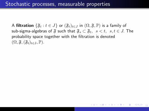
Stochastic processes, measurable properties
A filtration Ft : t ∈ J or (Ft)t∈J in (Ω,F,P) is a family ofsub-sigma-algebras of F such that Fs ⊂ Ft, s < t, s, t ∈ J. Theprobability space together with the filtration is denoted(Ω,F, (Ft)t∈J,P).
We say that the process Xt : t ∈ J is
measurable if X : J × Ω→ S is B(J)⊗ F-measurable.
adapted to the filtration Ft : t ∈ J if for all t ∈ J , Xt isFt-measurable.
progressively measurable or simply progressive if for allt > 0 the function (s, ω)→ S from [0, t]× Ω to S isB[0, t]⊗ Ft measurable.
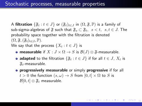
11
Stochastic processes, measurable properties
A filtration Ft : t ∈ J or (Ft)t∈J in (Ω,F,P) is a family ofsub-sigma-algebras of F such that Fs ⊂ Ft, s < t, s, t ∈ J. Theprobability space together with the filtration is denoted(Ω,F, (Ft)t∈J,P).We say that the process Xt : t ∈ J is
measurable if X : J × Ω→ S is B(J)⊗ F-measurable.
adapted to the filtration Ft : t ∈ J if for all t ∈ J , Xt isFt-measurable.
progressively measurable or simply progressive if for allt > 0 the function (s, ω)→ S from [0, t]× Ω to S isB[0, t]⊗ Ft measurable.

12
Stochastic processes
These definitions are interesting in the continuous time setting. Inthe discrete time case, all we usually need is that the process isadapted in the space (Ω,F, (Fn)n∈J,P).
The canonical filtration of a given process Xt : t ∈ J is thefiltration generated by the process, i.e, for each t ∈ J , Ft is thesigma algebra generated by the family of random variablesXs : s ≤ t, s ∈ J, which can also be written as
(Ft = σ(Xs : s ∈ J, s ≤ t), t ∈ J.)
It is obvious that any process is adapted to its canonical filtration.

12
Stochastic processes
These definitions are interesting in the continuous time setting. Inthe discrete time case, all we usually need is that the process isadapted in the space (Ω,F, (Fn)n∈J,P).The canonical filtration of a given process Xt : t ∈ J is thefiltration generated by the process, i.e, for each t ∈ J , Ft is thesigma algebra generated by the family of random variablesXs : s ≤ t, s ∈ J, which can also be written as
(Ft = σ(Xs : s ∈ J, s ≤ t), t ∈ J.)
It is obvious that any process is adapted to its canonical filtration.

13
Stochastic processes
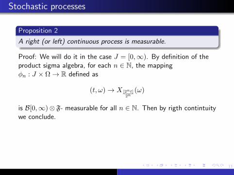
Proposition 2
A right (or left) continuous process is measurable.
Proof: We will do it in the case J = [0,∞). By definition of theproduct sigma algebra, for each n ∈ N, the mappingφn : J × Ω→ R defined as
(t, ω)→ X [2nt]2n
(ω)
is B[0,∞)⊗ F- measurable for all n ∈ N. Then by rigth contintuitywe conclude.The same idea is used to prove the following result:
Proposition 3
* A right (or left) continuous adapted process is progressive.
13
Stochastic processes
Proposition 2
A right (or left) continuous process is measurable.
Proof: We will do it in the case J = [0,∞). By definition of theproduct sigma algebra, for each n ∈ N, the mappingφn : J × Ω→ R defined as
(t, ω)→ X [2nt]2n
(ω)
is B[0,∞)⊗ F- measurable for all n ∈ N. Then by rigth contintuitywe conclude.
The same idea is used to prove the following result:
Proposition 3
* A right (or left) continuous adapted process is progressive.

13
Stochastic processes
Proposition 2
A right (or left) continuous process is measurable.
Proof: We will do it in the case J = [0,∞). By definition of theproduct sigma algebra, for each n ∈ N, the mappingφn : J × Ω→ R defined as
(t, ω)→ X [2nt]2n
(ω)
is B[0,∞)⊗ F- measurable for all n ∈ N. Then by rigth contintuitywe conclude.The same idea is used to prove the following result:
Proposition 3
* A right (or left) continuous adapted process is progressive.
14
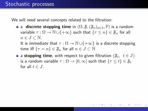
Stochastic processes
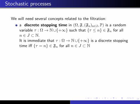
We will need several concepts related to the filtration:
a discrete stopping time in (Ω,F, (Fn)n∈J,P) is a randomvariable τ : Ω→ N∪+∞ such that τ ≤ n ∈ Fn for alln ∈ J ⊂ N.It is immediate that τ : Ω→ N∪+∞ is a discrete stoppingtime iff τ = n ∈ Fn for all n ∈ J ⊂ N
a stopping time, with respect to given filtration (Ft, t ∈ J)is a random variable τ : Ω→ [0,∞] such that τ ≤ t ∈ Ftfor all t ∈ J .
Given a stopping time τ and a process X, the mappingXτ : Ω→ S is defined as
Xτ (ω) := Xτ(ω)(ω).
14
Stochastic processes
We will need several concepts related to the filtration:
a discrete stopping time in (Ω,F, (Fn)n∈J,P) is a randomvariable τ : Ω→ N∪+∞ such that τ ≤ n ∈ Fn for alln ∈ J ⊂ N.It is immediate that τ : Ω→ N∪+∞ is a discrete stoppingtime iff τ = n ∈ Fn for all n ∈ J ⊂ Na stopping time, with respect to given filtration (Ft, t ∈ J)is a random variable τ : Ω→ [0,∞] such that τ ≤ t ∈ Ftfor all t ∈ J .
Given a stopping time τ and a process X, the mappingXτ : Ω→ S is defined as
Xτ (ω) := Xτ(ω)(ω).
15
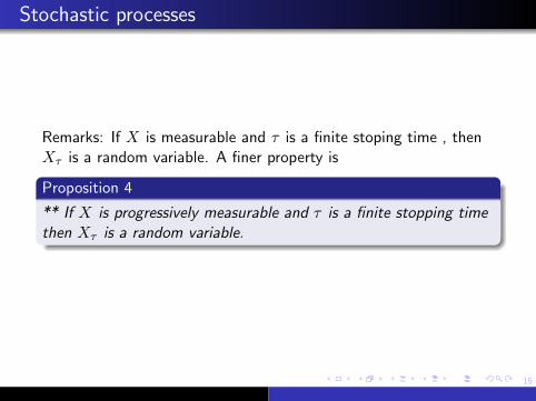
Stochastic processes
Remarks: If X is measurable and τ is a finite stoping time , thenXτ is a random variable. A finer property is
Proposition 4
** If X is progressively measurable and τ is a finite stopping timethen Xτ is a random variable.
16
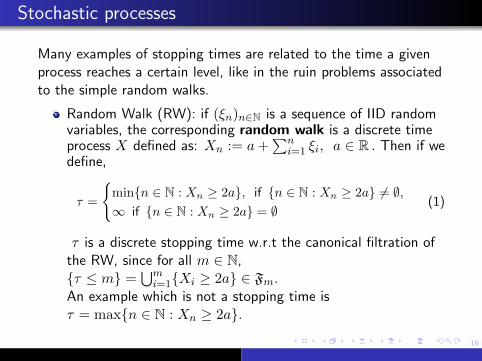
Stochastic processes
Many examples of stopping times are related to the time a givenprocess reaches a certain level, like in the ruin problems associatedto the simple random walks.
Random Walk (RW): if (ξn)n∈N is a sequence of IID randomvariables, the corresponding random walk is a discrete timeprocess X defined as: Xn := a+
∑ni=1 ξi, a ∈ R . Then if we
define,
τ =
minn ∈ N : Xn ≥ 2a, if n ∈ N : Xn ≥ 2a 6= ∅,∞ if n ∈ N : Xn ≥ 2a = ∅
(1)
τ is a discrete stopping time w.r.t the canonical filtration ofthe RW, since for all m ∈ N,τ ≤ m =
⋃mi=1Xi ≥ 2a ∈ Fm.
An example which is not a stopping time isτ = maxn ∈ N : Xn ≥ 2a.

17
Stochastic processes
In fact, a similar result is true if we replace the R.W. by anyadapted discrete time process.
*If X = (Xt : t ≥ 0) is a process with continuous paths and Ais a closed subset of R then the hitting time of a set A isdefined as:
TA =
inft ≥ 0 : Xt ∈ A, if t ≥ 0 : Xt ∈ A 6= ∅,∞ if t ≥ 0 : Xt ∈ A = ∅
(2)
It can be proved that it is a stopping time.

18
Martingales
A martingale defined in (Ω,F, (Ft)t∈J,P) is a stochastic processXt : t ∈ J such that
Xt : t ∈ J is adapted to the given filtration,
for all t ∈ J , E(|Xt|) <∞for all s, t ∈ J such that s < t the following condition isfulfilled:
E(Xt|Fs) = Xs.
Martingales form a very important class of processes, as will beseen in the development of this course. A submartingale (resp.supermartingale) verifies the first two properties andE(Xt|Fs) ≥ Xs. (resp. E(Xt|Fs) ≤ Xs.)We have the properties like s→ E(Xs) is constant for amartingale because, for s < t,
E(Xt) = E(E(Xt|Fs)) = E(Xs).

19
Martingales
Some examples are:
1. In the random walk if E(ξ1) = 0, then
Xn = a+
n∑i=1
ξi
is a martingale with respect to the canonical filtration (Fn)n∈Nand is called discrete time martingale.If E(ξ1) ≥ 0 (or E(ξ1) ≤ 0) the corresponding random walk is asubmartingale ( supermartingale) with respect to the canonicalfiltration.
2. Any process Xt : t ∈ [0, T ] such that
E(Xt) = 0 t ≥ 0,Xt+s −Xs and Fs are independent, for all s, t ≥ 0
is a martingale with respect to the canonical filtration,(Ft)t

20
Martingales
To see this we simply write, in the first case,
E(Xn+m|Fn) = E
[[Xn +
m∑i=n+1
ξi] |Fn
]= Xn.
We used the facts:
the independence between (ξi)mi=n+1 and Fn,
the knowledge that Xn is Fn-measurable,
the hypothesis E(ξi) = 0 for all i ∈ N.
For the second example, observe thatE(Xt+s −Xs|Fs) = E(Xt+s −Xs) = 0, because of theindependence between Xt+s −Xs and Fs.
21
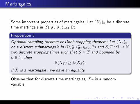
Martingales
Some important properties of martingales. Let (Xn)n be a discretetime martingale in (Ω,F, (Fn)n∈J,P).
Proposition 5
Optional sampling theorem or Doob stopping theorem: Let (Xn)nbe a discrete submartingale in (Ω,F, (Fn)n∈J,P) and S, T : Ω→ Ntwo discrete stopping times such that S ≤ T and bounded byk ∈ N, then
E(XT ) ≥ E(XS).
If X is a martingale , we have an equality.
Observe that for discrete time martingales, XT is a randomvariable.

22
Martingales
Idea of the proof: Ω =⋃kj=0(S = j) and it is a disjoint union; so
we can write XS as XS(ω) =∑k
j=0Xj1(S=j)(ω).We shall only prove a special case since this is the case we willneed: T ≡ k and S ≤ k.
XT −XS =
k∑j=0
(Xk −Xj)1(S=j) =
k−1∑j=0
(Xk −Xj)1(S=j)
and this sum has positive expectation (or is zero in the martingalecase), since the set (S = j) ∈ Fj , we get
E[1(S=j)(Xk −Xj)
]≥ 0, j = 0, 1, . . . (k − 1).

23
Martingales
Proposition 6
Let (X)Nn=0, be a discrete positive submartingale in(Ω,F, (Fn)n∈J,P), then for all λ > 0
P(supnXn ≥ λ ≤
1
λE(XN .1(supnXn≥λ)) ≤
1
λE(|XN |).
24
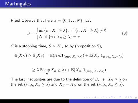
Martingales
Proof:Observe that here J = 0, 1 . . . N. Let
S =
infn : Xn ≥ λ, if n : Xn ≥ λ 6= ∅N if n : Xn ≥ λ = ∅
(3)
S is a stopping time, S ≤ N , so by (proposition 5),
E(XN ) ≥ E(XS) = E(XS .1(supnXn≥λ)) + E(XS .1(supnXn<λ))
≥ λP(supnXn ≥ λ) + E(XN .1(supnXn<λ))
The last inequalities are due to the definition of S, i.e. XS ≥ λ onthe set (supnXn ≥ λ) and XS = XN on the set (supnXn ≤ λ).

25
Martingales
For a discrete time martingale X, we then have ( by JensenInequality) a positive submartingale (|Xn|p : n ∈ 0, 1, 2 . . . N)whenever E(|XN |p) <∞ and in any case we obtain:
Corollary 1
If X is a discrete time martingale indexed by the finite set0, 1, 2 . . . N and if p ≥ 1 then
λp P[supn|Xn| ≥ λ
]≤ E(|XN |p), λ > 0

26
Martingales
The former properties can be extended to the continuous time case:
Theorem 1
Doob’s maximal inequality: Let (Mt)t≥0 be a right continuousmartingale and p ≥ 1 then
P( sup0≤s≤t
|Ms| ≥ λ) ≤ 1
λpE(|Mt|p), t ≥ 0, λ > 0.
Proof. . Let D be a countable dense subset of the interval [0, t].Because of the right continuity
sups∈D|Ms| = sup
s∈[0,t]|Ms|.
27
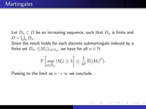
Martingales
Let Dn ⊂ D be an increasing sequence, such that Dn is finite andD =
⋃nDn.
Since the result holds for each discrete submartingale indexed by afinite set Dn, (|Ms|)s∈Dn , we have for all n ∈ N
P[
sups∈Dn
|Ms| ≥ λ]≤ 1
λpE(|Mt|P ).
Passing to the limit as n→∞ we conclude.

28
Gaussian random variables
Definition 1
The normal random variable X : Ω→ R with mean m andvariance σ2 (X ≈ N (m,σ2)), has density
1
(2πσ2)1/2exp
[−(x−m)2
2σ2
]Some useful properties on gaussian or normal random variables:
a.- if m = 0, E(X2) = σ2, E(X4) = 3σ4,
b.- var(X2) = E[X2 − σ2
]2= 2σ4.
c.- ψ(λ) = E [exp(λX)] = exp(λm+ σ2λ2
2 ) (Laplace transform).
d.- ΦX(u) = E [exp(iuX)] = exp(imu− σ2u2
2 )(Characteristic function.)(Excercise).
29
Brownian motion
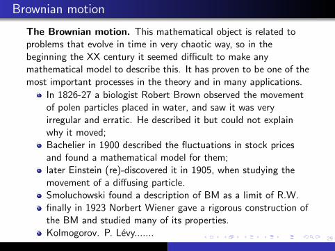
The Brownian motion. This mathematical object is related toproblems that evolve in time in very chaotic way, so in thebeginning the XX century it seemed difficult to make anymathematical model to describe this. It has proven to be one of themost important processes in the theory and in many applications.
In 1826-27 a biologist Robert Brown observed the movementof polen particles placed in water, and saw it was veryirregular and erratic. He described it but could not explainwhy it moved;Bachelier in 1900 described the fluctuations in stock pricesand found a mathematical model for them;later Einstein (re)-discovered it in 1905, when studying themovement of a diffusing particle.Smoluchowski found a description of BM as a limit of R.W.finally in 1923 Norbert Wiener gave a rigorous construction ofthe BM and studied many of its properties.Kolmogorov. P. Levy.......

30
Brownian motion
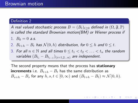
Definition 2
A real valued stochastic process B = (Bt)t≥0 defined in (Ω,F,P)is called the standard Brownian motion(BM) or Wiener process if
1. B0 = 0 a.s.
2. Bt+h −Bt has N (0, h) distribution, for 0 ≤ h and 0 ≤ t.3. For all n ∈ N and all times 0 ≤ t1 < t2 < . . . < tn the random
variables (Bti −Bti−1)(i=1,2...n) are independent.
The second property means that the process has stationaryincrements i.e. Bt+h −Bt has the same distribution asBs+h −Bs for any h, s, t ∈ [0,∞) and (Bt+h −Bt) ≈ N (0, h).The third condition can also be stated as: for all t, s > 0, therandom variable Bt+s −Bt is independent of Fs = σBu : u ≤ s.
30
Brownian motion
Definition 2
A real valued stochastic process B = (Bt)t≥0 defined in (Ω,F,P)is called the standard Brownian motion(BM) or Wiener process if
1. B0 = 0 a.s.
2. Bt+h −Bt has N (0, h) distribution, for 0 ≤ h and 0 ≤ t.3. For all n ∈ N and all times 0 ≤ t1 < t2 < . . . < tn the random
variables (Bti −Bti−1)(i=1,2...n) are independent.
The second property means that the process has stationaryincrements i.e. Bt+h −Bt has the same distribution asBs+h −Bs for any h, s, t ∈ [0,∞) and (Bt+h −Bt) ≈ N (0, h).
The third condition can also be stated as: for all t, s > 0, therandom variable Bt+s −Bt is independent of Fs = σBu : u ≤ s.

30
Brownian motion
Definition 2
A real valued stochastic process B = (Bt)t≥0 defined in (Ω,F,P)is called the standard Brownian motion(BM) or Wiener process if
1. B0 = 0 a.s.
2. Bt+h −Bt has N (0, h) distribution, for 0 ≤ h and 0 ≤ t.3. For all n ∈ N and all times 0 ≤ t1 < t2 < . . . < tn the random
variables (Bti −Bti−1)(i=1,2...n) are independent.
The second property means that the process has stationaryincrements i.e. Bt+h −Bt has the same distribution asBs+h −Bs for any h, s, t ∈ [0,∞) and (Bt+h −Bt) ≈ N (0, h).The third condition can also be stated as: for all t, s > 0, therandom variable Bt+s −Bt is independent of Fs = σBu : u ≤ s.
31
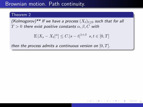
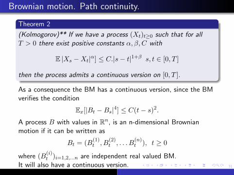
Brownian motion. Path continuity.
Theorem 2
(Kolmogorov)** If we have a process (Xt)t≥0 such that for allT > 0 there exist positive constants α, β, C with
E |Xs −Xt|α] ≤ C.|s− t|1+β s, t ∈ [0, T ]
then the process admits a continuous version on [0, T ].
As a consequence the BM has a continuous version, since the BMverifies the condition
Ex[|Bt −Bs|4] ≤ C(t− s)2.
A process B with values in Rn, is an n-dimensional Brownianmotion if it can be written as
Bt = (B(1)t , B
(2)t , . . . B
(n)t ), t ≥ 0
where (B(i)t )i=1,2,...n are independent real valued BM.
It will also have a continuous version.
31
Brownian motion. Path continuity.
Theorem 2
(Kolmogorov)** If we have a process (Xt)t≥0 such that for allT > 0 there exist positive constants α, β, C with
E |Xs −Xt|α] ≤ C.|s− t|1+β s, t ∈ [0, T ]
then the process admits a continuous version on [0, T ].
As a consequence the BM has a continuous version, since the BMverifies the condition
Ex[|Bt −Bs|4] ≤ C(t− s)2.
A process B with values in Rn, is an n-dimensional Brownianmotion if it can be written as
Bt = (B(1)t , B
(2)t , . . . B
(n)t ), t ≥ 0
where (B(i)t )i=1,2,...n are independent real valued BM.
It will also have a continuous version.

32
Brownian motion
Another definition of Brownian motion is
Definition 3
A real valued stochastic process B = (Bt)t≥0 defined in (Ω,F,P)is called Brownian motion or Wiener process if
A. Is a Gaussian Process.
B. m(t) = E(Bt) = 0, t ≥ 0,
C. cov(Bt, Bs) = C(s, t) = min(s, t), s, t ≥ 0

33
Brownian motion
We now see one of the implications. The other one is left as anexcercise.If B verifies definition 2 then ,
A. It is a Gaussian process: given n ∈ N, 0 ≤ t1 ≤ t2 ≤ . . . tn forany ai ∈ R, i = 1, 2, . . . n, then there exist bi ∈ R, i = 1, 2, . . . nverifying
n∑i=1
aiBti =
n∑i=1
bi(Bti −Bti−1).
B. m(t) = 0, t ≥ 0 and
C. for 0 ≤ s < t
cov(Bs, Bt)= E(BsBt) =E(Bs(Bt −Bs) +B2s )= s
since E(Bs)E(Bt −Bs) = 0 and E(B2s ) = s.
so it verifies definition 3.
34
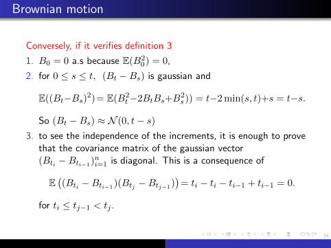
Brownian motion
Conversely, if it verifies definition 3
1. B0 = 0 a.s because E(B20) = 0,
2. for 0 ≤ s ≤ t, (Bt −Bs) is gaussian and
E((Bt−Bs)2)= E(B2t−2BtBs+B
2s )) = t−2 min(s, t)+s = t−s.
So (Bt −Bs) ≈ N (0, t− s)3. to see the independence of the increments, it is enough to prove
that the covariance matrix of the gaussian vector(Bti −Bti−1)ni=1 is diagonal. This is a consequence of
E((Bti −Bti−1)(Btj −Btj−1)
)= ti − ti − ti−1 + ti−1 = 0.
for ti ≤ tj−1 < tj .

35
Gaussian processes
Proposition 7
Given a function m : [0, T ]→ R and a symmetric positive definitefunction C : [0, T ]× [0, T ]→ R there exists a probability space(Ω,F,P) and Gaussian process (Xt)t∈[0,T ] defined on it such thatit has mean function m and covariance function C.
This result is based in Daniel-Kolmogorov existence theorem andon properties of Gaussian vectors.

36
Brownian motion
The existence of the BM is a consequence of the formerproposition for Gaussian processes. This is done taking the meanfunction as m(t) = 0, t ≥ 0 and the covariance function asC(s, t) = cov(Bs, Bt) = min(s, t), s, t ≥ 0.
All we must verify is that this function is positive definite(symmetry is immediate). So for any n ∈ N, si ∈ R+ andai ∈ R, i = 1, 2 . . . n,∑
1≤i,j≤naiajC(si, sj) =
∑1≤i,j≤n
aiaj
∫ ∞0
1[0,si)(s)1[0,sj)(s)ds =
∫ ∞0
( n∑i=1
ai1[0,si)(s))2ds ≥ 0

36
Brownian motion
The existence of the BM is a consequence of the formerproposition for Gaussian processes. This is done taking the meanfunction as m(t) = 0, t ≥ 0 and the covariance function asC(s, t) = cov(Bs, Bt) = min(s, t), s, t ≥ 0.All we must verify is that this function is positive definite(symmetry is immediate). So for any n ∈ N, si ∈ R+ andai ∈ R, i = 1, 2 . . . n,∑
1≤i,j≤naiajC(si, sj) =
∑1≤i,j≤n
aiaj
∫ ∞0
1[0,si)(s)1[0,sj)(s)ds =
∫ ∞0
( n∑i=1
ai1[0,si)(s))2ds ≥ 0
37
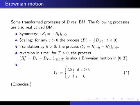
Brownian motion
Some transformed processes of B real BM. The following processesare also real valued BM:
Symmetry: (Zt = −Bt)t≥0
Scaling: for any c > 0 the process (Bct = 1
cBc2t : t ≥ 0)
Translation by h > 0: the process (Yt = Bt+h −Bh)t≥0.
reversion in time: for T > 0, the process(RTt = BT −BT−t)t∈[0,T ] is also a Brownian motion in [0, T ].
Yt :=
tB 1
tif t > 0
0 if t = 0.(4)
(Excercise:)

38
Brownian motion
The following process associated to the Brownian motion(Bt : t ≥ 0) are martingales with respect to canonical filtration ofthe BM.
1. (Bt : t ≥ 0)
2. (B2t − t : t ≥ 0)
3. For any a ∈ R,(Mt = exp(aBt − a2
2 t) : t ≥ 0).

39
Brownian motion
Proofs: Let 0 ≤ s < t.
1. E(Bt −Bs|Fs) = E(Bt −Bs) = 0
2. E(B2t −B2
s − (t− s)|Fs) =E((Bt −Bs)2 − (t− s) + 2Bs(Bt −Bs)|Fs
)= 0
3.
E(Mt|Fs
)= Ms iff E
(Mt
Ms|Fs)
= 1
and this last conditional expectation equals (using theproperties of Gaussian r.v)
E[exp(a(Bt −Bs))− a2
2 (t− s))|Fs]
=
exp(−a2
2 (t− s))E [exp(a(Bt −Bs)] = 1

40
Brownian motion
We also consider the BM started at point y ∈ R. It is thetranslated process (y +Bt : t ≥ 0). We use the notationsEy(.), Py(.) for the expectation and the probability in this case.
For A ∈ B(R) the definition of BM gives us the distribution ofeach Bt,
P(Bt ∈ A) =
∫Ap(x, 0, t)dx =
1
(2πt)1/2
∫A
exp
[−x
2
2t
]dx,
Py(Bt ∈ A) =
∫Ap(x, y, t)dx =
1
(2πt)1/2
∫A
exp
[−(x− y)2
2t
]dx,
and for any borel- measurable and bounded function f : R→ R,
Ey(f(Bt)) =
∫f(x)p(x, y, t)dx =
1
(2πt)1/2
∫f(x) exp
[−(x− y)2
2t
]dx,

40
Brownian motion
We also consider the BM started at point y ∈ R. It is thetranslated process (y +Bt : t ≥ 0). We use the notationsEy(.), Py(.) for the expectation and the probability in this case.For A ∈ B(R) the definition of BM gives us the distribution ofeach Bt,
P(Bt ∈ A) =
∫Ap(x, 0, t)dx =
1
(2πt)1/2
∫A
exp
[−x
2
2t
]dx,
Py(Bt ∈ A) =
∫Ap(x, y, t)dx =
1
(2πt)1/2
∫A
exp
[−(x− y)2
2t
]dx,
and for any borel- measurable and bounded function f : R→ R,
Ey(f(Bt)) =
∫f(x)p(x, y, t)dx =
1
(2πt)1/2
∫f(x) exp
[−(x− y)2
2t
]dx,

41
Brownian motion
Computation of joint probabilities.
Theorem 3
For n ∈ N, 0 ≤ t1 ≤ t2 ≤ . . . tn and f : Rn → R, bounded andmeasurable,
E[f(Bt1 , Bt2 , . . . Btn)] =
∫ +∞
−∞. . .
∫ +∞
−∞f(x1, x2, . . . xn).
.p(x1, 0, t1)p(x2, x1, t2−t1) . . . p(xn, xn−1, tn−tn−1)dxn . . . dx2dx1
and
Ex[f(Bt1 , Bt2 , . . . Btn)] =
∫ +∞
−∞. . .
∫ +∞
−∞f(x1, x2, . . . xn).
.p(x1, x, t1)p(x2, x1, t2−t1) . . . p(xn, xn−1, tn−tn−1)dxn . . . dx2dx1

42
Brownian motion
Idea: there exists a linear transformation T : Rn → Rn such that
h(y1, . . . , yn) := f(T (y1, . . . , yn)) = f(y1, y1+y2, . . . , y1+y2, · · ·+yn)
then define Yi = Bti −Bti−1 , i = 1, 2, . . . n which are independent,so they have a joint density,p(y1, 0, t1)p(y2, 0, t2 − t1) . . . p(yn, 0, tn − tn−1) and
E[f(Bt1 , Bt2 , . . . Btn)] = E[h(Yt1 , Yt2 , . . . Ytn)]∫ +∞
−∞. . .
∫ +∞
−∞h(y1, y2, . . . yn).
.p(y1, 0, t1)p(y2, 0, t2 − t1) . . . p(yn, 0, tn − tn−1)dyn . . . dy2 dy1
Since the jacobian of T equals 1, we can transform this integral inorder to obtain the result.

43
Brownian motion: Markov property
Theorem 4
Let B be a standard Brownian motion. For a borel and boundedfunction, f : R→ R and 0 ≤ s ≤ t
1. E(f(Bt)|Fs) = E(f(Bt)|Bs),
2. E [f(Bt)|σ(Bs)] = 1(2π(t−s))1/2
∫R f(x) exp
[− (x−Bs)2
2(t−s)
]dx,
3. E(f(Bt)|Bs = y) = 1(2π(t−s))1/2
∫R f(x) exp
[− (x−y)2
2(t−s)
]dx,
44
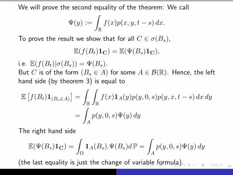
We will prove the second equality of the theorem: We call
Ψ(y) :=
∫Rf(x)p(x, y, t− s) dx.
To prove the result we show that for all C ∈ σ(Bs),
E(f(Bt)1C) = E(Ψ(Bs)1C),
i.e. E(f(Bt)|σ(Bs)) = Ψ(Bs).But C is of the form (Bs ∈ A) for some A ∈ B(R). Hence, the lefthand side (by theorem 3) is equal to
E[f(Bt)1(Bs∈A)
]=
∫R
∫Rf(x)1A(y)p(y, 0, s)p(y, x, t− s) dx dy
=
∫Ap(y, 0, s)Ψ(y) dy
The right hand side
E(Ψ(Bs)1C) =
∫Ω1A(Bs).Ψ(Bs)dP =
∫Ap(y, 0, s)Ψ(y) dy
(the last equality is just the change of variable formula).
45
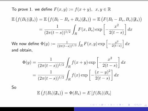
To prove 1. we define F (x, y) := f(x+ y), x, y ∈ R
E(f(Bt)|Fs)
)= E
(f(Bt −Bs +Bs)|Fs)
)= E
(F (Bt −Bs, Bs)|Fs)
)=
1
(2π(t− s))1/2
∫RF (x,Bs) exp
[− x2
2(t− s)
]dx
We now define Φ(y) := 1(2π(t−s))1/2
∫R F (x, y) exp
[− x2
2(t−s)
]dx
and obtain,
Φ(y) =1
(2π(t− s))1/2
∫Rf(x+ y) exp
[− x2
2(t− s)
]dx
=1
(2π(t− s))1/2
∫Rf(x) exp
[−(x− y)2
2(t− s)
]dx
SoE(f(Bt)|Fs)
)= Φ(Bs) = E [f(Bt)|Bs]
46
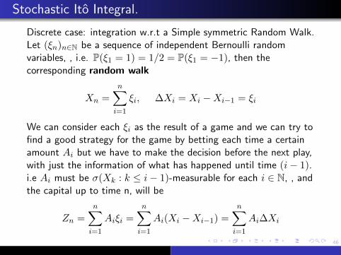
Stochastic Ito Integral.
Discrete case: integration w.r.t a Simple symmetric Random Walk.Let (ξn)n∈N be a sequence of independent Bernoulli randomvariables, , i.e. P(ξ1 = 1) = 1/2 = P(ξ1 = −1), then thecorresponding random walk
Xn =
n∑i=1
ξi, ∆Xi = Xi −Xi−1 = ξi
We can consider each ξi as the result of a game and we can try tofind a good strategy for the game by betting each time a certainamount Ai but we have to make the decision before the next play,with just the information of what has happened until time (i− 1).i.e Ai must be σ(Xk : k ≤ i− 1)-measurable for each i ∈ N, , andthe capital up to time n, will be
Zn =
n∑i=1
Aiξi =
n∑i=1
Ai(Xi −Xi−1) =
n∑i=1
Ai∆Xi
47
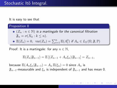
Stochastic Ito Integral.
It is easy to see that
Proposition 8
(Zn : n ∈ N) is a martingale for the canonical filtrationFn = σ(Xk : k ≤ n).
E(Zn) = 0, var(Zn) =∑n
i=1 E(A2i ) if An ∈ L2 (Ω,F,P)
Proof: It is a martingale: for any n ∈ N,
E(Zn|Fn−1) = E [(Zn−1 +Anξn)|Fn−1] = Zn−1,
because E(Anξn|Fn−1) = An E(ξn) = 0 since An isFn−1-measurable and ξn is independent of Fn−1 and has mean 0.

48
Stochastic Ito Integral.
To compute its variance:
E(Z2n)=E(
n∑i,j
AiAjξiξj)=E(
n∑i
A2i ξ
2i )=
n∑i
E(A2i )E(ξ2
i )=
n∑i
E(A2i ),
we used:
for the second equality, if i < j,
E(AiAjξiξj)=E(E(AiAjξiξj |Fj−1)) =
= E(AiAjξi E(ξj |Fj−1)) = E(AiAjξi E(ξj)) =0,
because of the measurability and independence assumed.
for the third one, Ai depends only on (ξk : k = 1, 2...i− 1)and these are independent of ξi
E(ξ2i ) = 1.

49
Stochastic Ito Integral.
More generally, given a discrete Martingale (Xn)n∈N, in(Ω,F, (Fn)n∈J,P) and a bounded positive process (An)n such thatAn is Fn−1 measurable, n = 1, 2 . . . we can define the stochasticintegral ( also called the martingale transform of A) as:
(A ·X)n = Zn =
n∑i=1
Ai(Xi −Xi−1) =
n∑i=1
Ai∆Xi.
It can be proved that it is also a martingale and we can computeits variance (left as exercise).

50
Stochastic Ito Integral.
We want to give sense to
Zt =∫ t
0 g(s)dBs, for g : R→ R,to∫h(Xs)dBs for a process (Xs : s ≥ 0).
or to∫H(s,Xs)dBs for a process (Xs : s ≥ 0).
for convenient classes of functions g, h,H and processes X. Thefirst one is rather easy to study ( the Paley-Wiener integral,
defined as −∫ T
0 g′(t)Btdt, for g differentiable and such thatg(0) = g(T ) = 0) but the second one, will prove to be quite trickydue to the great irregularity of the paths of the Brownian motiont→ Bt, as will be seen in the next slides.
51
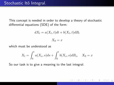
Stochastic Ito Integral.
This concept is needed in order to develop a theory of stochasticdifferential equations (SDE) of the form:
dXt = a(Xt, t)dt+ b(Xt, t)dBt
X0 = x
which must be understood as
Xt =
∫ t
0a(Xs, s)ds+
∫ t
0b(Xs, s)dBs, X0 = x
So our task is to give a meaning to the last integral.

52
Stochastic Ito Integral.
A simple case: we will try to compute∫ t
0 BdB: a Riemann sumfor it would be ∑
π
Brk(Btk+1−Btk)
where π is a partition: 0 = t0 < t1 < . . . tm = t of [0, t] andrk ∈ [tk, tk+1]. Since ( as will be seen later) the Brownian motionhas paths with unbounded variation, we cannot expect to obtain apathwise limit .We will see that different choices of the intermediate point giverise to different limits. First we will study the variation of thebrownian paths.
53
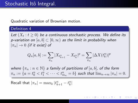
Stochastic Ito Integral.
Quadratic variation of Brownian motion.
Definition 4
Let (Xt : t ≥ 0) be a continuous stochastic process. We define itsp-variation on [a, b] ⊂ [0,∞) as the limit in probability when|πn| → 0 (if it exist) of
Qn[a, b] :=∑πn
|Xtnk+1−Xtnk
|p =∑πn
|∆X(tnk)|p
where πn : n ∈ N a family of partitions of [a, b], of the formπn := a = tn0 < tn1 < · · · < tnmn
= b such that limn→∞ |πn| = 0.
Recall that |πn| = maxk |tnk+1 − tnk |
54
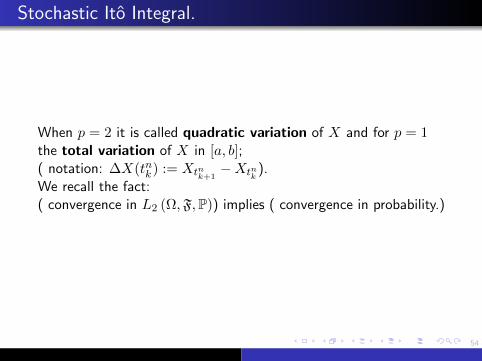
Stochastic Ito Integral.
When p = 2 it is called quadratic variation of X and for p = 1the total variation of X in [a, b];( notation: ∆X(tnk) := Xtnk+1
−Xtnk).
We recall the fact:( convergence in L2 (Ω,F,P)) implies ( convergence in probability.)

55
Stochastic Ito Integral.
Proposition 9
The quadratic variation on [0, t] of the Brownian motion, B isequal to t and is denoted < B,B >t.
Let πn : n ∈ N be a family of partitions of [a, b], of the formπn := a = tn0 < tn1 < · · · < tnmn
= b, such that limn→∞ |πn| = 0.
We will use the result: If X ≈ N (0, σ2) then var(X2) = 2σ4.So if ∆B(tnk) := Btnk+1
−Btnk , ∆tnk := (tnk+1 − tnk) then
∆B(tnk) ≈ N (0,∆tnk) and var[(∆B(tnk))2] = 2(∆tnk)2.

56
Stochastic Ito Integral.
We will prove that
[L2− lim
n→∞Qn
]=
[L2− lim
n→∞
∑πn
(∆B(tnk))2
]= (b− a).
E[(Qn − (b− a))2] = E
[(∑πn
∆B(tnk)2 −∆tnk)2
]=
This is the variance of a sum of independent random variables, soit is equal to the sum of the variances:
=∑πn
var[∆B(tnk)2 −∆tnk
]= 2
∑πn
(∆tnk)2 ≤ 2|πn|.(b− a),
and since |πn| → 0 as n→∞, the former goes to 0.The case stated in the proposition is for a = 0, b = t.

57
Stochastic Ito Integral.
Corollary 2
1.-If 1 ≤ p < 2 the p-variation of the BM is a.s. infinite.2.- The total variation of the paths of BM is a.s infinite.
Idea: We will work the case (a, b) = (0, t) and we suppose that Bhas finite p-variation for some p ∈ [1, 2) and let δ = 2− p > 0,∑
πnk
|Btnk+1−Btnk |
2 =∑πnk
|Btnk+1−Btnk |
2−δ|Btnk+1−Btnk |
δ
≤ supπnk
|Btnk+1−Btnk |
δ.∑πn
|Btnk+1−Btnk |
p.
This inequality leads to a contradiction.

58
Stochastic Ito Integral.
We return to the example∫ t
0 BdB:
Lemma 1
Let (πn)n be sequence of a partitions of [0, t] with the samenotations and λ ∈ [0, 1] fixed. We define
Rn(λ) =∑πn
Brnk ∆B(tnk)
with rnk = (1− λ)tnk + λtnk+1. Then
L2 − limn→∞
Rn(λ) =B2t
2+ (λ− 1/2)t.
This means that the limit of the Riemann sum depends on theintermediate point rnk selected and there is a rule to choose it.

59
Stochastic Ito Integral.
An easy ( but long computation) shows that for a partitionπn := 0 = tn0 < tn1 < · · · < tnmn
= t, Rn can be written as
Rn =B2
t2 +An +Bn + Cn with
An = −1/2∑πn
(∆B(tnk))2, and An → −t/2 in the L2 norm.
Bn =∑πn
(Brnk −Btnk )2, and Bn → λt in the L2 norm
Cn =∑πn
(Btnk+1−Brnk )(Brnk −Btnk ) and using properties of
the independence of the increments, we get E(C2n)→ 0

60
Stochastic Ito Integral.
We will do in detail the case λ = 0, i.e. rnk = tnk :
Rn(0) =∑πn
Btnk ∆B(tnk) =1
2
∑πn
[(B2
tnk+1−B2
tnk)− (Btnk+1
−Btnk )2]
the first term is a telescopic sum and is equal toB2
t2 and we
already know that the second converges in L2 to
− t2
and this gives rise to the Ito Stochastic Integral , which is theone we will develop here and what we just computed is .
(B ·B)t :=
∫ t
0BdB =
∫ t
0BsdBs =
B2t
2− t
2

61
Stochastic Ito Integral.
The case λ = 1/2 according to the lemma is equal to:
Rn(1/2)→ B2t
2,
which is also used and is called the Stratonovich Integral.
Observe that:(B2
t2 −
t2 , t ≥ 0) is a martingale while the
Stratonovich integralB2
t2 , is not.

62
Stochastic Ito Integral.
For technical reasons we will work with the completed canonicalfiltration for the BM, (Ft)t.
Definition 5
Given a filtered space (Ω,F, (Ft)t∈J,P), and 0 ≤ a < b the classΓ2[a, b] is the set of processes F : [0,∞)× Ω→ R such that
F is progressively measurable
E[∫ ba F (s, ω)2ds
]is finite.

63
Stochastic Ito Integral.
Definition 6
A process G defined in (Ω,F, (Ft)t∈J,P) is called elementaryprocesses if it belongs to Γ2[0, T ] and there exists a partitionπ = 0 = t0 < t1 < · · · < tm = T and random variablesGk : Ω→ R, k = 0, 1, 2 . . .m− 1 such that
G(t, ω) = Gk(ω), for t ∈ [tk, tk+1), k = 0, 1, . . . ,m− 1.
The set of elementary processes in [0, T ] will be denoted E [0, T ].
64
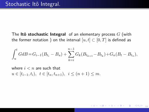
Stochastic Ito Integral.
The Ito stochastic Integral of an elementary process G (withthe former notation ) on the interval [u, t] ⊂ [0, T ] is defined as∫ t
uGdB=Gi−1(Bti −Bu) +
n−1∑k=i
Gk(Btk+1−Btk)+Gn(Bt −Btn),
where i < n are such thatu ∈ [ti−1, ti), t ∈ [tn, tn+1), i ≤ (n+ 1) ≤ m.

65
Stochastic Ito Integral.
Observe
E(G2k) <∞ and Gk is Ftk -measurable, k = 1, 2 . . .m− 1
since the process is adapted (analogy with the bettingstrategy for RW).
if i = n i.e. if both points u, t belong to the same interval ofthe partition then
∫ tu GdB = Gi−1(Bt −Bu)
(G ·B)t is an usual notation for the stochastic integral∫ t0 GdB.
we can also write:∫ tu GdB = (G1[u,t] ·B)T∫ T
0 GdB is also the martingale transform of (Gk)k ( seen as adiscrete process) w.r.t. the martingale(Xn = Btn , n = 1, 2, . . .m)
Notice that we could also have defined a elementary processwithout using the space Γ2[0, T ].

66
Stochastic Ito Integral.
Proposition 10
For G,G1, G2 ∈ E [0, T ], the stochastic integral
is additive:∫ tu GdB =
∫ su GdB +
∫ ts GdB. 0 ≤ u < s < t < T
is linear:∫ t0 (aG1 + bG2)dB = a
∫ t0 G1dB + b
∫ t0 G2dB, a, b ∈ R
verifies E(∫ t
0 GdB) = 0.
the stochastic integral as a process:(Zt :=
∫ t0 GdB : t ∈ [0, T ]) is a continuous square integrable
martingale.
67
Stochastic Ito Integral.The Ito Isometry
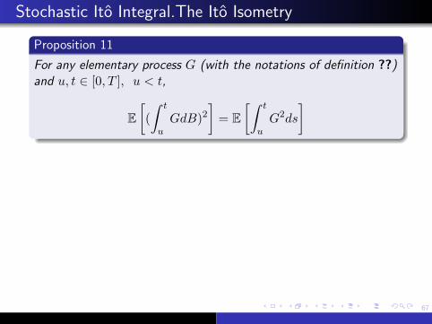
Proposition 11
For any elementary process G (with the notations of definition ??)and u, t ∈ [0, T ], u < t,
E[(
∫ t
uGdB)2
]= E
[∫ t
uG2ds
]
We do it in the case u = 0, t = T and use the notation∆Bk := B(tk+1)−B(tk).
E [∆Bk] = 0 and
E[(∆Bk)
2]
= (tk+1 − tk),k 6= j, j < k.
E [GkGj∆Bk∆Bj ] = E [GkGj∆Bj ]E [∆Bk] = 0,
k = j,
E[G2k(∆Bk)
2]
= E[G2k
]E[(∆Bk)
2]
= E(G2k)(tk+1 − tk)

67
Stochastic Ito Integral.The Ito Isometry
Proposition 11
For any elementary process G (with the notations of definition ??)and u, t ∈ [0, T ], u < t,
E[(
∫ t
uGdB)2
]= E
[∫ t
uG2ds
]We do it in the case u = 0, t = T and use the notation∆Bk := B(tk+1)−B(tk).
E [∆Bk] = 0 and
E[(∆Bk)
2]
= (tk+1 − tk),k 6= j, j < k.
E [GkGj∆Bk∆Bj ] = E [GkGj∆Bj ]E [∆Bk] = 0,
k = j,
E[G2k(∆Bk)
2]
= E[G2k
]E[(∆Bk)
2]
= E(G2k)(tk+1 − tk)

68
Stochastic Ito Integral.The Ito Isometry
Now we use these results to compute:
E[(
∫ T
0GdB)2
]=∑j,k
E [GkGj∆Bk∆Bj ] =∑k
E(G2k)(tk+1 − tk)
which is equal to E[∫ T
0 G2ds]. This proves the Ito isometry for
elementary processes.For the case u, t ∈ [0, T ] we can do exactly the same with themodified partition π = u = t0 < t1 < · · · < tn = t or else do itfor the elementary processes G1[u,t].
Observe that E[∫ TO G2ds
]is the L2([0, T ]× Ω)-norm of G.

69
Stochastic Ito Integral.
The class of elementary processes E [0, T ] is a subset of the productspace L2(([0, T ]× Ω),A, µ) where A is the product sigma algebraB([0, T ])⊗ F and µ is the product measure λ× P, with λ theLebesgue measure in B([0, T ]).
Theorem 5
The closure of E [0, T ] with respect to the norm in the productspace L2(([0, T ]× Ω) is Γ2[0, T ].
Idea of the proof: the measurability conditions are preserved sincean L2- limit admits a subsequence that is a.s. convergent.Now , given a process X in Γ2[0, T ] the method to find thesequence of elementary processes that converge in the productspace to X relies on a deterministic lemma:

70
Stochastic Ito Integral.
Lemma 2
Deterministic lemma: In the space L2[0, T ] of functionsf : [0, T ]→ R we define the operator Pn : L2[0, T ]→ L2[0, T ] by
Pnf(t) =
n∑j=1
[ξj−11[tj−1,tj)
], ξj−1 =
n
T
∫ tj−1
tj−2
f(s)ds
with (tj)nj=0 the uniform partition of [0, T ]: (tj = jT
n ). Then
1- for φ a step function in L2[0, T ], limn |Pnφ− φ|2 = 0,
2- the set of step functions is a dense subset of L2[0, T ]
3- if ψ ∈ L2[0, T ] then limn |Pnψ − ψ|2 = 0.

71
Stochastic Ito Integral.
Lemma 3
Deterministic lemma: In the space L2[0, T ] of functionsf : [0, T ]→ R we define the operator Pn : L2[0, T ]→ L2[0, T ] by
Pnf(t) =n∑j=1
[ξj−11[tj−1,tj)
], ξj−1 =
n
T
∫ tj−1
tj−2
f(s)ds
with (tj)nj=0 the uniform partition of [0, T ]: (tj = jT
n ). Then
1- for φ a bounded continuous function in [0, T ],limn |Pnφ− φ|2 = 0,
2- the set of bounded continuous functions is a dense subset ofL2[0, T ]
3- if ψ ∈ L2[0, T ] then limn |Pnψ − ψ|2 = 0.
72
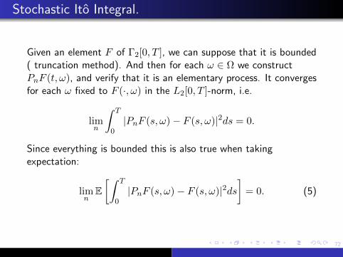
Stochastic Ito Integral.
Given an element F of Γ2[0, T ], we can suppose that it is bounded( truncation method). And then for each ω ∈ Ω we constructPnF (t, ω), and verify that it is an elementary process. It convergesfor each ω fixed to F (·, ω) in the L2[0, T ]-norm, i.e.
limn
∫ T
0|PnF (s, ω)− F (s, ω)|2ds = 0.
Since everything is bounded this is also true when takingexpectation:
limn
E[∫ T
0|PnF (s, ω)− F (s, ω)|2ds
]= 0. (5)

73
Stochastic Ito Integral.
We call Gn = PnF ∈ Γ2[0, T ] . Thanks to equation (5), (Gn)n isa Cauchy sequence in the product space L2([0, T ]×Ω) and thanksto the Ito isometry for elementary processes, for any t ∈ [0, T ], thesequence (
∫ t0 GndB)n is a Cauchy sequence in L2 (Ω,F,P) :
E[|∫ t
0GndB −
∫ t
0GmdB|2
]= E
[|∫ t
0(Gn −Gm)dB|2
]= E
[∫ t
0(Gn −Gm)2dt
]
74
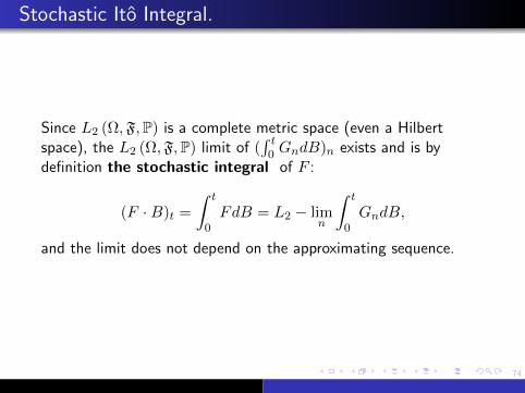
Stochastic Ito Integral.
Since L2 (Ω,F,P) is a complete metric space (even a Hilbertspace), the L2 (Ω,F,P) limit of (
∫ t0 GndB)n exists and is by
definition the stochastic integral of F :
(F ·B)t =
∫ t
0FdB = L2 − lim
n
∫ t
0GndB,
and the limit does not depend on the approximating sequence.
75
Stochastic Ito Integral.
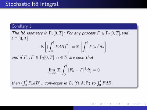
Corollary 3
The Ito Isometry in Γ2[0, T ]: For any process F ∈ Γ2[0, T ],andt ∈ [0, T ],
E[(
∫ t
0FdB)2
]= E
[∫ t
0F (s)2ds
]and if Fn, F ∈ Γ2[0, T ] n ∈ N are such that
limn→∞
E[
∫ t
0|Fn − F |2dt] = 0
then (∫ t
0 FndB)n converges in L2 (Ω,F,P) to∫ t
0 FdB.

76
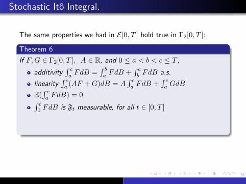
Stochastic Ito Integral.
The same properties we had in E [0, T ] hold true in Γ2[0, T ]:
Theorem 6
If F,G ∈ Γ2[0, T ], A ∈ R, and 0 ≤ a < b < c ≤ T ,
additivity∫ ca FdB =
∫ ba FdB +
∫ cb FdB a.s.
linearity∫ ca (AF +G)dB = A
∫ ca FdB +
∫ ca GdB
E(∫ ca FdB) = 0∫ t
0 FdB is Ft measurable, for all t ∈ [0, T ]
((f ·B)t =∫ t
0 FdB : t ∈ [0, T ]) is a continuous squareintegrable martingale.
The proof is based in the fact that these results are true forelementary processes. The last one needs special attention:

76
Stochastic Ito Integral.
The same properties we had in E [0, T ] hold true in Γ2[0, T ]:
Theorem 6
If F,G ∈ Γ2[0, T ], A ∈ R, and 0 ≤ a < b < c ≤ T ,
additivity∫ ca FdB =
∫ ba FdB +
∫ cb FdB a.s.
linearity∫ ca (AF +G)dB = A
∫ ca FdB +
∫ ca GdB
E(∫ ca FdB) = 0
∫ t0 FdB is Ft measurable, for all t ∈ [0, T ]
((f ·B)t =∫ t
0 FdB : t ∈ [0, T ]) is a continuous squareintegrable martingale.
The proof is based in the fact that these results are true forelementary processes. The last one needs special attention:
76
Stochastic Ito Integral.
The same properties we had in E [0, T ] hold true in Γ2[0, T ]:
Theorem 6
If F,G ∈ Γ2[0, T ], A ∈ R, and 0 ≤ a < b < c ≤ T ,
additivity∫ ca FdB =
∫ ba FdB +
∫ cb FdB a.s.
linearity∫ ca (AF +G)dB = A
∫ ca FdB +
∫ ca GdB
E(∫ ca FdB) = 0∫ t
0 FdB is Ft measurable, for all t ∈ [0, T ]
((f ·B)t =∫ t
0 FdB : t ∈ [0, T ]) is a continuous squareintegrable martingale.
The proof is based in the fact that these results are true forelementary processes. The last one needs special attention:

76
Stochastic Ito Integral.
The same properties we had in E [0, T ] hold true in Γ2[0, T ]:
Theorem 6
If F,G ∈ Γ2[0, T ], A ∈ R, and 0 ≤ a < b < c ≤ T ,
additivity∫ ca FdB =
∫ ba FdB +
∫ cb FdB a.s.
linearity∫ ca (AF +G)dB = A
∫ ca FdB +
∫ ca GdB
E(∫ ca FdB) = 0∫ t
0 FdB is Ft measurable, for all t ∈ [0, T ]
((f ·B)t =∫ t
0 FdB : t ∈ [0, T ]) is a continuous squareintegrable martingale.
The proof is based in the fact that these results are true forelementary processes. The last one needs special attention:

77
Stochastic Ito Integral:The Ito integral as a process.
Theorem 7
For F ∈ Γ2[0, T ], the process defined by
(t, ω)→∫ t
0FdB, t ∈ [0, T ]
admits a continuous version and it is a square integrablemartingale.
Proof:Let (Gn) be the sequence of elementary process thatapproximate F in Γ2[0, T ] and we take any t ∈ [0, T ].
Each∫ t
0 GndB is a continuous martingale, and so∫ t0 GndB −
∫ t0 GmdB is also a continuous martingale for any
n,m ∈ N.

77
Stochastic Ito Integral:The Ito integral as a process.
Theorem 7
For F ∈ Γ2[0, T ], the process defined by
(t, ω)→∫ t
0FdB, t ∈ [0, T ]
admits a continuous version and it is a square integrablemartingale.
Proof:Let (Gn) be the sequence of elementary process thatapproximate F in Γ2[0, T ] and we take any t ∈ [0, T ].Each
∫ t0 GndB is a continuous martingale, and so∫ t
0 GndB −∫ t
0 GmdB is also a continuous martingale for anyn,m ∈ N.

78
Stochastic Ito Integral: the Ito integral as a process.
Thanks to the Doob maximal inequality for martingales (theorem1) :
P
(sup
0≤t≤T
∣∣∣∣∫ t
0GndB −
∫ t
0GmdB
∣∣∣∣ > ε
)
≤ 1
ε2E
(∣∣∣∣∫ t
0GndB −
∫ t
0GmdB
∣∣∣∣2)
=1
ε2E(∫ t
0(Gn −Gm)2ds
)→ 0, n,m→∞.

79
Stochastic Ito Integral: the Ito integral as a process.
So we can find a subsequence (nk) such that
P(Ak) := P
[sup
0≤t≤T
∣∣∣∣∫ t
0Gnk+1
dB −∫ t
0Gnk
dB
∣∣∣∣ > 2−k
]≤ 2−k
And by the Borel Cantelli lemma
P(lim supAk) = 0
This means that for almost all ω ∈ Ω there exists k1(ω) such thatfor k ≥ k1
sup0≤t≤T
∣∣∣∣(∫ t
0Gnk+1
dB −∫ t
0Gnk
dB)(ω)
∣∣∣∣ ≤ 2−k, k ≥ k1
So a.s we get uniform convergence. Since t→∫ t
0 GndB iscontinuous, the limit is also continuous. It is a martingale becauseit is the L2-limit of martingales. It is clearly square integrablebecause of the Ito isometry.

80
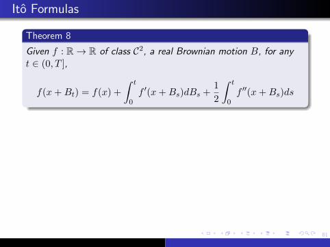
Ito Formulas
As we have seen the computation of stochastic integrals is noteasy. The Ito formula allows us to compute many more and it isfundamental in the theory, and is the main tool for the study ofSDE. We will give the main ideas of two classical forms of provingthe theorem.The first approach to the simples Ito formula is using the Taylorexpansion:
81
Ito Formulas
Theorem 8
Given f : R→ R of class C2, a real Brownian motion B, for anyt ∈ (0, T ],
f(x+Bt) = f(x) +
∫ t
0f ′(x+Bs)dBs +
1
2
∫ t
0f ′′(x+Bs)ds
We will do the case when f, f ′ and f ′′ are bounded by a constantM ∈ R+ and are uniformly continuous. Let πn be a partition of[0, t] given by 0 = tn0 ≤ tn1 , . . . ≤ tnmn
= t. We can use the Taylorformula to obtain
f(x+Bt) = f(x) +∑πn
f ′(x+Btnj )[Btnj+1−Btnj ]
+1/2∑πn
f ′′(x+Btnj )[Btnj+1−Btnj ]2 +Rn
82
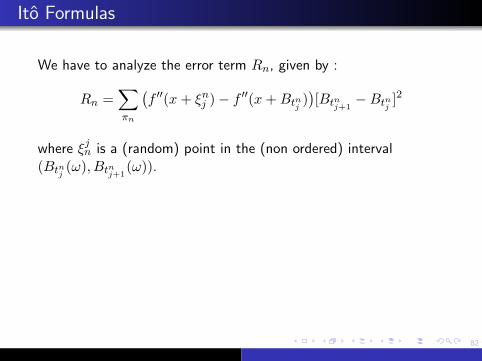
Ito Formulas
We have to analyze the error term Rn, given by :
Rn =∑πn
(f ′′(x+ ξnj )− f ′′(x+Btnj )
)[Btnj+1
−Btnj ]2
where ξjn is a (random) point in the (non ordered) interval(Btnj (ω), Btnj+1
(ω)).
We also use the notations:
An =∑πn
f ′′(x+Btnj )[Btnj+1−Btnj ]2, Bn =
∑πn
f ′′(x+Btnj )[tnj+1−tnj ]
Ln(j) = f ′′(x+Btnj )[(Btnj+1−Btnj )2 − (tnj+1 − tnj )],
∆B(tnj ) = (Btnj+1−Btnj ), j = 1, 2 . . . (mn − 1)

82
Ito Formulas
We have to analyze the error term Rn, given by :
Rn =∑πn
(f ′′(x+ ξnj )− f ′′(x+Btnj )
)[Btnj+1
−Btnj ]2
where ξjn is a (random) point in the (non ordered) interval(Btnj (ω), Btnj+1
(ω)).We also use the notations:
An =∑πn
f ′′(x+Btnj )[Btnj+1−Btnj ]2, Bn =
∑πn
f ′′(x+Btnj )[tnj+1−tnj ]
Ln(j) = f ′′(x+Btnj )[(Btnj+1−Btnj )2 − (tnj+1 − tnj )],
∆B(tnj ) = (Btnj+1−Btnj ), j = 1, 2 . . . (mn − 1)
83
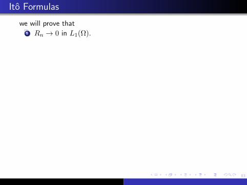
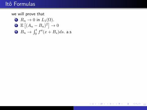
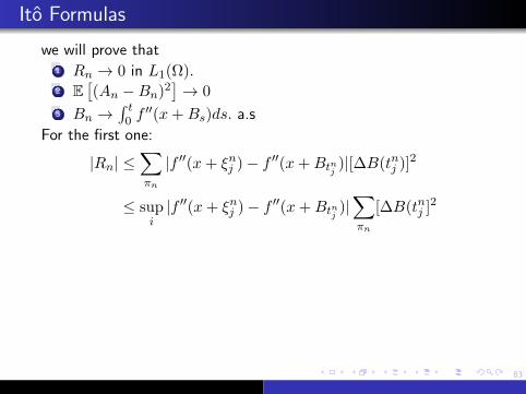
Ito Formulas
we will prove that1 Rn → 0 in L1(Ω).
2 E[(An −Bn)2
]→ 0
3 Bn →∫ t
0 f′′(x+Bs)ds. a.s
For the first one:
|Rn| ≤∑πn
|f ′′(x+ ξnj )− f ′′(x+Btnj )|[∆B(tnj )]2
≤ supi|f ′′(x+ ξnj )− f ′′(x+Btnj )|
∑πn
[∆B(tnj ]2
Using the Cauchy -Schwarz inequality
[E(Rn)]2≤E
[sup
j|f ′′(x+ξnj )−f ′′(x+Btnj )|2
]E
[∑πn
[∆B(tnj )]22]

83
Ito Formulas
we will prove that1 Rn → 0 in L1(Ω).2 E
[(An −Bn)2
]→ 0
3 Bn →∫ t
0 f′′(x+Bs)ds. a.s
For the first one:
|Rn| ≤∑πn
|f ′′(x+ ξnj )− f ′′(x+Btnj )|[∆B(tnj )]2
≤ supi|f ′′(x+ ξnj )− f ′′(x+Btnj )|
∑πn
[∆B(tnj ]2
Using the Cauchy -Schwarz inequality
[E(Rn)]2≤E
[sup
j|f ′′(x+ξnj )−f ′′(x+Btnj )|2
]E
[∑πn
[∆B(tnj )]22]

84
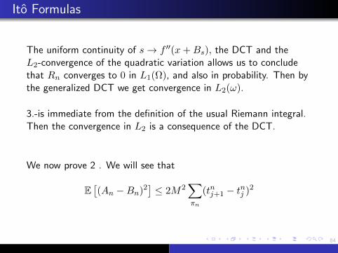
Ito Formulas
The uniform continuity of s→ f ′′(x+Bs), the DCT and theL2-convergence of the quadratic variation allows us to concludethat Rn converges to 0 in L1(Ω), and also in probability. Then bythe generalized DCT we get convergence in L2(ω).
3.-is immediate from the definition of the usual Riemann integral.Then the convergence in L2 is a consequence of the DCT.
We now prove 2 . We will see that
E[(An −Bn)2
]≤ 2M2
∑πn
(tnj+1 − tnj )2
84
Ito Formulas
The uniform continuity of s→ f ′′(x+Bs), the DCT and theL2-convergence of the quadratic variation allows us to concludethat Rn converges to 0 in L1(Ω), and also in probability. Then bythe generalized DCT we get convergence in L2(ω).
3.-is immediate from the definition of the usual Riemann integral.Then the convergence in L2 is a consequence of the DCT.
We now prove 2 . We will see that
E[(An −Bn)2
]≤ 2M2
∑πn
(tnj+1 − tnj )2

85
Ito Formulas
E[(An −Bn)2
]= E
[[∑πn
Ln(j)]2
]= E
∑j,k
Ln(j)Ln(k)
=
= E[∑
j Ln(j)2]≤M2 E
[∑πn
((Btnj+1
−Btnj )2 − (tnj+1 − tnj ))2]
= 2M2∑
πn(tnj+1 − tnj )2
For the last equality we used the fact that the ifY ≈ N (0, tnj+1 − tnj ), then E(Y 2) = 2(tnj+1 − tnj )2.

85
Ito Formulas
E[(An −Bn)2
]= E
[[∑πn
Ln(j)]2
]= E
∑j,k
Ln(j)Ln(k)
=
= E[∑
j Ln(j)2]≤M2 E
[∑πn
((Btnj+1
−Btnj )2 − (tnj+1 − tnj ))2]
= 2M2∑
πn(tnj+1 − tnj )2
For the last equality we used the fact that the ifY ≈ N (0, tnj+1 − tnj ), then E(Y 2) = 2(tnj+1 − tnj )2.

86
Ito Formulas
The same method can be used to prove a similar result for timedependent functions: f : (R+)× R→ R of class C1,2,
f(t, x+Bt) = f(0, x)+
∫ t
0f ′x(s, x+Bs)dBs+
1
2
∫ t
0f ′′xx(s, x+Bs)ds+
+
∫ t
0f ′t(s, x+Bs)ds.
87
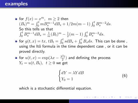
examples
for f(x) = xm, m ≥ 2 then(Bt)
m =∫ t
0 mBm−1s dBs + 1/2m(m− 1)
∫ t0 B
m−2s ds.
So this tells us that∫ t0 B
m−1s dBs = 1
m(Bt)m − 1
2(m− 1)∫ t
0 Bm−2s ds.
for g(t, x) = tx, tBt =∫ t
0 sdBs +∫ t
0 Bsds. This can be done ,using the Ito formula in the time dependent case , or it can beproved directly.
for u(t, x) = exp(λx− λ2t2 ) and defining the process
Yt = u(t, Bt), t ≥ 0 we getdY = λY dB
Y0 = 1(6)
which is a stochastic differential equation.

88
Ito Processes
Definition 7 ( Ito Processes.)
Given (Ω,F, (Ft)t∈J,P) , an Ito process is a process of the form
Xt = X0 +
∫ t
0A(ω, s)ds+
n∑j=1
∫ t
0Gj(ω, s)dB
js
with
Gj ∈ Γ2[0, T ] j = 1, 2 . . . n,
A is a progressive integrable process,
X0 ∈ L2(Ω) and F0-measurable
Bt = (B(1)t , B
(2)t , . . . B
(n)t ) an Rn -valued Brownian motion.
In differential form this is written as :
dXt = Ads+∑j
GjdB(j)

89
Ito Processes
This family of processes is a subspace of the set of continuoussemimartingales, it is the sum of continuous martingales∫ t
0 Aj(ω, s)dBs and a bounded variation continuous process∫ t0 b(ω, s)ds. We want to see if we have also an Ito formula for this
family of processes, i.e. if we can compute f(Xt) for functions f(with enough regularity conditions). Notice that(f(Xt) : t ∈ [0, T ]) is a new process, and we will see that it willalso be an Ito process.
90
Ito Formula
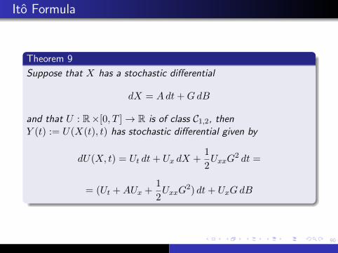
Theorem 9
Suppose that X has a stochastic differential
dX = Adt+GdB
and that U : R×[0, T ]→ R is of class C1,2, thenY (t) := U(X(t), t) has stochastic differential given by
dU(X, t) = Ut dt+ Ux dX +1
2UxxG
2 dt =
= (Ut +AUx +1
2UxxG
2) dt+ UxGdB
91
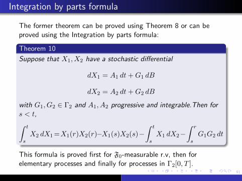
Integration by parts formula
The former theorem can be proved using Theorem 8 or can beproved using the Integration by parts formula:
Theorem 10
Suppose that X1, X2 have a stochastic differential
dX1 = A1 dt+G1 dB
dX2 = A2 dt+G2 dB
with G1, G2 ∈ Γ2 and A1, A2 progressive and integrable.Then fors < t,∫ t
sX2 dX1 =X1(r)X2(r)−X1(s)X2(s)−
∫ t
sX1 dX2−
∫ r
sG1G2 dt
This formula is proved first for F0-measurable r.v, then forelementary processes and finally for processes in Γ2[0, T ].

92
higher dimensions
Definition 8
An Mn×m-valued process , G= (Gi,j)i=1,...n,j=1,...m belongs toΓn×m2 [0, T ] if each Gi,j ∈ Γ2[0, T ].An Rn valued process F= (Fi)i=1,...n), belongs to Γn1 [0, T ] if each
component Fi is progressive and verifies E∫ T
0 |Fi(s)|ds is finite.
In this case we can also construct∫ T
0GdBt.
(here B is an m-dimensional Brownian motion.) We also havemultidimensional Ito processes and Ito Chain rule.
93
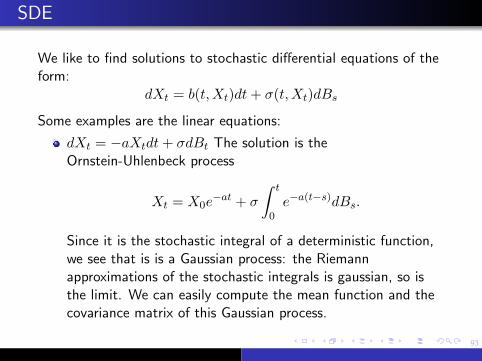
SDE
We like to find solutions to stochastic differential equations of theform:
dXt = b(t,Xt)dt+ σ(t,Xt)dBs
Some examples are the linear equations:
dXt = −aXtdt+ σdBt The solution is theOrnstein-Uhlenbeck process
Xt = X0e−at + σ
∫ t
0e−a(t−s)dBs.
Since it is the stochastic integral of a deterministic function,we see that is is a Gaussian process: the Riemannapproximations of the stochastic integrals is gaussian, so isthe limit. We can easily compute the mean function and thecovariance matrix of this Gaussian process.

94
The Vasicek model:dXt = (−aXt + b)dt+ σdBt. has asolution given by
Xt = X0e−at + b/a(1− e−at)σ
∫ t
0e−a(t−s)dBs.
dZt = Ztφ(t)dBt with φ bounded and progressive. Thesolution is
Zt = Z0 exp
[∫ t
0φ(s)dBs −
1
2
∫φ(s)2ds
]dZt = Zt [µ(t)dt+ φ(t)dBt] where µ and φ are bounded andprogressive and Z0 = 1. The solution is
Zt = exp
[∫ t
0µ(s)ds+
∫ t
0φ(s)dBs −
1
2
∫φ(s)2ds
]

95
What do we mean by a solution?? A solution X of
dXt = b(t,Xt)dt+ σ(t,Xt)dBs, X0 = X(0) t ∈ [0, T ]
is a progressive process , b and σ progressive, such theb ∈ L1 (Ω,F,P) and σ ∈ Γ2[0, T ] and for all times t ∈ [0, T ],
Xt = X0 +
∫ t
0b(t,Xt)dt+
∫ t
0σ(t,Xt)dBs.

96
Stratonovich Integral
∫ t
0H • dB =
∫ t
0HdB +
1
2
∫ t
0Hxdt

97
Bibliography
Lawrence C. Evans : An introduction to Stochasticdifferential equations. AMS (2013).
Bernt Oksendal: Stochastic differentialequations.Springer (2000)
D. Revuz, M. Yor : Continuous Martingales andBrownian motion. Springer (1999)
Rene L. Schilling, Lothar Partzsch: Brownianmotion. De Gruyter (2012.)


