Introduction to structured equations in biology · PDF fileIntroduction to structured...

Introduction to structured equations in biology

Benoıt Perthameemail: [email protected]

Ecole Normale Superieure

Departement de Mathematiques et Applications, CNRS UMR 8553

45 rue d’Ulm, 75230 Paris Cedex 05, France

Chapter 1

Examples of stage structuredpopulation equations

Population biology is certainly the oldest area of biology where mathematics hasbeen used. Speaking usually of large populations, partial differential equations(PDE) play a natural role. The recent book of H. Thieme [16] gives a generalview of this subject.

This Chapter presents several examples of stage structured equations, mostlybased on the Lecture Note by the author [14].

1.1 The renewal equation: demography and cell

division cycle

1.1.1 Setting the model

The simplest model to understand why other variables than space can enter naturallyin PDE models of biology is certainly the renewal equation for demography. Considera ’closed’ population with no immigration, neither emigration. Neglect also for thetime being death and consider only aging and birth.

The population density n(t, x) of individuals of age x > 0 at time t then satisfies

n(t+ s, x+ s) = n(t, x), ∀s ≥ 0.

As a consequence, differentiating in s, and taking s = 0, we find

∂

∂tn(t, x) +

∂

∂xn(t, x) = 0 t ≥ 0, x ≥ 0, . (1.1)

This equation has to be complemented by the ’boundary condition’ at x = 0, i.e.the number of newborns at time t; this is given by the quantity

n(t, x = 0) =

∫ ∞

0

B(y)n(t, y)dy, (1.2)

3

4 Examples of stage structured population equations

where B denotes the birth rate of the population (that vanishes certainly for x ≈ 0and x large).

These two last equations form the so-called renewal equation. They were intro-duced by McKendrick for epidemiology, then x denotes the age in the disease, animportant factor for the epidemic spread.

The same model was re-discovered some years later by von Foerster [18] for thecell division cycle. In this context it is natural stipulate that cells, after division,take some time x∗, with a well reported variability, before dividing again. We arrivewith the variant of the previous renewal equation

∂∂tn(t, x) + ∂

∂xn(t, x) + k(x)n(t, x) = 0, t ≥ 0, x ≥ 0,

n(t, x = 0) = 2∫k(y)n(t, y)dy,

n(t = 0, x) = n0(x).

(1.3)

Here k(x) denotes the division rate. A possible choice is

k(x) = A1I{x≥x∗}.

1.1.2 Age structured equations and Volterra equations

Consider the system (1.3) and set

K(x) =

∫ x

0

k(y)dy.

Therefore∂

∂t[eK(x)n(t, x)] +

∂

∂x[eK(x)n(t, x)] = 0, t ≥ 0, x ≥ 0,

and eK(x)n(t, x) is constant along the characteristics eK(x−s)n(t−s, x−s) = eK(x)n(t, x).We choose successively s = x and s = t

eK(x)n(t, x) =

n(t− x, 0) = b(t− x), x < t,

eK(x−t)n0(x− t), x > t.

Inserting this information and defining b(t) as the birth term

b(t) = n(t, x = 0), (1.4)

we find the so-called Volterra integral equationb(t) = 2

∫k(y)e−K(y)b(t− y)dy + b0(t),

b0(t) = 2∫k(y)eK(y−t)−K(y)n0(y − t).

(1.5)

This equation can be solved by the standard Cauchy-Lipschitz theory.

1.2. FINITE RESOURCES AND NONLINEARITIES 5

1.1.3 The limit of deterministic birth age

In order to simplify the analysis, it is often assumed the division occurs exactly ata certain age x∗. This means we are now interested in the limit A → ∞ for thefollowing division rate

k(x) = kA(y) = A1I{x≥x∗}.

Then, the weight kA(y)e−KA(y) ≥ 0 has the following properties∫ ∞

0

kA(y)e−KA(y)dy = 1, kA(y)e−KA(y) = 0 for y < x∗,

kA(y)e−KA(y) = Ae−A(y−x∗) −−−−−→A→∞ 0, for y > x∗.

Therefore, we have : kA(y)e−KA(y) −−−−−→A→∞ δ(a− x∗).

Inserting this in (1.5) gives, in the limit A→∞ (after passing to the limit alsoin b0A(t)),

b(t) = 2b(t− x∗) + b0(t),

1.2 Finite resources and nonlinearities

We give two examples of nonlinearities which we take from two different areas ofbiosciences: ecology and epidemiology.

1.2.1 A nonlinear model from ecology

Nonlinear models are typically possible when including a limited resource S(t) sharedby all the population. The level of nutrient controls growth, death and birth. Thisyields models as

∂∂tn(t, x) + ∂

∂x

[(xm

S(t)1+S(t)

− x)n(t, x)]+ d(x, S(t))n(t, x) = 0,

n(t, x = 0) =∫B(y, S(t))n(t, y)dy,

n(t = 0, x) = n0(x),

(1.6)

here we take naturally 0 ≤ x ≤ xm. If x represents the size of the micro-organismunder consideration, this equation expresses that x increases as long as the nutrientlevel is high enough and diminishes when it is too low for maintening the organismwhich needs are proportional to it size x.

This PDE is coupled with a differential equation for the resources which expressestheir outflow (degration), inflow (with rate S0), their consumption For instance onecan write a balance law

d

dtS(t) + S(t) = S0 − S(t)

1 + S(t)

∫ xm

0

x2n(t, x)dx. (1.7)


It is also usual to assume that the resources are available with a faster time scale(adiabatic assumption). Then, we replace the differential equation on S(t) by itssteady state, the mere algebraic equation

S(t) +S(t)

1 + S(t)

∫ xm

0

x2n(t, x)dx = S0.

1.2.2 The Kermack-McKendrick model for epidemic spread

Ordinary differential equations have been used for a long time to describe the spreadof an epidemy in a population. The simplest are called SIR (Susceptible, Infected,Resistant), an extension is the SEIR (Exposed) model, and reads

dSdt

= βS(S + I +R)− µSS − γSS I,

dIdt

= γSS I − µII − βRI,

dRdt

= βRI − µRR.

(1.8)

In order to improve the validity of the model, Kermack and McKendrick [10,8] proposed to take into account the variable infectivity level, and removal rate,depending on the age in the disease. They arrive at

d

dtS(t) = B − µSS(t)− λS(t)S(t),

λS(t) :=

∫ ∞

0

κ(x)n(t, x)dx,

∂∂tn(t, x) + ∂

∂xn(t, x) + (µI + βn(x))n(t, x) = 0,

n(t, x = 0) = λS(t)S(t),

d

dtR(t) =

∫ ∞

0

βn(x)n(t, x)dx.

The interpretation is that n(t, x) is the density of population at age x of infectionand this replaces the compartment I(t) in the SIR system (1.8). Individuals areinfected (at age x = 0 in the infection stage) from susceptible that are getting thevirus by encounter with infected at a rate λS(t) depending of the time x elapsedsince infection through a rate κ(x). Notice again the quadratic term for transitionfrom susceptible to infected. The advantage of the Kermack-McKendrick model isthat one can take into account

The book [3] is a very good and recent account of the subject.

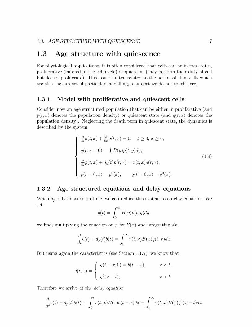
1.3. AGE STRUCTURE WITH QUIESCENCE 7

1.3 Age structure with quiescence

For physiological applications, it is often considered that cells can be in two states,proliferative (entered in the cell cycle) or quiescent (they perform their duty of cellbut do not proliferate). This issue is often related to the notion of stem cells whichare also the subject of particular modelling, a subject we do not touch here.

1.3.1 Model with proliferative and quiescent cells

Consider now an age structured population that can be either in prolifarative (andp(t, x) denotes the population density) or quiescent state (and q(t, x) denotes thepopulation density). Neglecting the death term in quiescent state, the dynamics isdescribed by the system

∂∂tq(t, x) + ∂

∂xq(t, x) = 0, t ≥ 0, x ≥ 0,

q(t, x = 0) =∫B(y)p(t, y)dy,

∂∂tp(t, x) + dp(t)p(t, x) = r(t, x)q(t, x),

p(t = 0, x) = p0(x), q(t = 0, x) = q0(x).

(1.9)

1.3.2 Age structured equations and delay equations

When dp only depends on time, we can reduce this system to a delay equation. Weset

b(t) =

∫ ∞

0

B(y)p(t, y)dy,

we find, multiplying the equation on p by B(x) and integrating dx,

d

dtb(t) + dp(t)b(t) =

∫ ∞

0

r(t, x)B(x)q(t, x)dx.

But using again the caracteristics (see Section 1.1.2), we know that

q(t, x) =

q(t− x, 0) = b(t− x), x < t,

q0(x− t), x > t.

Therefore we arrive at the delay equation

d

dtb(t) + dp(t)b(t) =

∫ t

0

r(t, x)B(x)b(t− x)dx+

∫ ∞

t

r(t, x)B(x)q0(x− t)dx.


0 1 2 3 4 5 60

0.1

0.2

0.3

0.4

0.5

0.6

0.7

Figure 1.1: Top:Experimental data for size distribution in E. coli. Bottom: Numer-

ical simulation of equation (1.10).

1.4 Size structured models (equal mitosis)

Size is usually a better physiological trait to structure cell populations as bacteriumor yeast. Then x is the mass (or length, or volume) of the cell. Assuming equalmitosis, i.e., that cells divide exactly in two equal new cells, the equation reads asfollows (for t ≥ 0, x ≥ 0),

∂∂tn(t, x) + ∂

∂x

[g(x)n(t, x)

]+B(x)n(t, x) = 4B(2x)n(t, 2x),

n(t, x = 0) = 0,

n(t = 0, x) = n0(x).

(1.10)

The term[g(x)n(t, x)

]describes the growth of cells using the (unlimited) nutrients.

The term 4B(2x)n(t, 2x) describes the division of cells of size 2x in two cells of sizex, the term B(x)n(t, x) takes into account the loose of cells of size x that divide incells of size x/2.

The dynamics of this model is also characterized by a growth, both of total

1.5. SIZE STRUCTURED MODELS (ASYMMETRIC DIVISION) 9

biomass and number of cells. The first natural question is to find the growth expo-nent. The second question is to find the typical repartition of cells (we will showthat this concept makes sense) which results from the two opposite effects describedby the model; growth by the differential term and x decay by the algebraic term.

In order to show that this model exhibits growth, one can notice two idendities.The first one is to consider the total number of cells and compute (this is formal atthis level, assuming that one can integrate on the half line)

d

dt

∫ ∞

0

n(t, x)dx+

∫ ∞

0

B(x)n(t, x)dx =

∫ ∞

0

4B(2x)n(t, 2x)dx = 2

∫ ∞

0

B(x)n(t, x)dx,

therefored

dt

∫ ∞

0

n(t, x)dx =

∫ ∞

0

B(x)n(t, x)dx,

in words, this means that the total number of cells only increases thanks to thedivision rate B.

One can also compute the biomass. Multiplying by x and integrating by partswe calculate

ddt

∫ ∞

0

xn(t, x)dx−∫ ∞

0

g(x)n(t, x)dx+

∫ ∞

0

xB(x)n(t, x)dx =

∫ ∞

0

4 xB(2x)n(t, 2x)dx

=

∫ ∞

0

xB(x)n(t, x)dx,

therefored

dt

∫ ∞

0

xn(t, x)dx =

∫ ∞

0

g(x)n(t, x)dx,

in words, biomass only increases by use of nutrients.

1.5 Size structured models (asymmetric division)

The division is not always symmetric and a daughter cell can be much smaller thatthe mother cell. The above model can be generalized to tak ethis into account.We arrive at an equation also calles ’aggregation-fragmentation’ because it arises inphysics to describe such phenomena e.g. for polymers.

∂∂tn(t, x) + ∂

∂x

[g(x)n(t, x)

]+B(x)n(t, x) = 2

∫B(y)κ(x, y)n(t, y)dy,

n(t, x = 0) = 0,

n(t = 0, x) = n0(x).

(1.11)


Figure 1.2: Asymmetric cell division in yeast.

Here B(y) is the division rate of cells of sizes y and κ(x, y) is the probality that sucha cell gives a daughter cell of size x ≤ y. It is natural to assume that (i) daughtercells are smaller than the mother cell, (ii) the division event gives two cells exactly,(iii) the toal mass is conserved in the division. These are expresses by the idendities

κ(x, y) = 0 for x > y, (1.12)∫ ∞

0

κ(x, y)dx = 1, (1.13)∫ ∞

0

x κ(x, y)dx = y/2. (1.14)

Notice that this last equality is a consequence the first two and of the naturalsymmetry assumption

κ(x, y) = κ(y − x, x).

As an exercise, one can notice that the same relations as in Section 1.4 hold forgrowth of the number of cells and total biomass (still formally, assuming that onecan integrate on the half line)

d

dt

∫ ∞

0

n(t, x)dx =

∫ ∞

0

B(x)n(t, x)dx,

d

dt

∫ ∞

0

xn(t, x)dx =

∫ ∞

0

g(x)n(t, x)dx.

For various choices of κ we can recover models we have already encountered. Letus give examples.(i) The renewal (age structured) equation (1.1)–(1.2) can be recovered using,

κ(x, y) =1

2

(δ(x = 0) + δ(x = y)

). (1.15)

1.6. NONLINEAR AGGREGATION-FRAGMENTATION FOR PRION 11

(ii) Equal mitosis, as in section 1.4, is the special case

κ(x, y) = δ(x = y/2). (1.16)

(iii) Uniform division is the case

κ(x, y) =1

y1I{0≤x≤y}. (1.17)

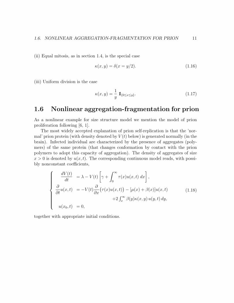
1.6 Nonlinear aggregation-fragmentation for prion

As a nonlinear example for size structure model we mention the model of prionproliferation following [6, 1].

The most widely accepted explanation of prion self-replication is that the ’nor-mal’ prion protein (with density denoted by V (t) below) is generated normally (in thebrain). Infected individual are characterized by the presence of aggregates (poly-mers) of the same protein (that changes conformation by contact with the prionpolymers to adopt this capacity of aggregation). The density of aggregates of sizex > 0 is denoted by u(x, t). The corresponding continuous model reads, with possi-bly nonconstant coefficients,

dV (t)

dt= λ− V (t)

[γ +

∫ ∞

0

τ(x)u(x, t) dx

],

∂

∂tu(x, t) = −V (t)

∂

∂x

(τ(x)u(x, t)

)− [µ(x) + β(x)]u(x, t)

+2∫∞

xβ(y)κ(x, y)u(y, t) dy,

u(x0, t) = 0,

(1.18)

together with appropriate initial conditions.


Chapter 2

Weak solutions to the renewalequation

In this Chapter we aim at building a solution in the weak (distribution) sense to therenewal equation

∂∂tn(t, x) + ∂

∂x[g(t, x)n(t, x)] + d(t, x)n(t, x) = 0, t ≥ 0, x ≥ 0,

g(t, 0) n(t, x = 0) =∫B(t, y)n(t, y)dy,

n(t = 0, x) = n0(x),

(2.1)

We assume that

0 ≤ d ∈ L∞(R+), 0 ≤ B ∈ L∞(R+), (2.2)

g(t, x) ∈ C1b(R+ × R+), g(t, 0) ≥ gm > 0, (2.3)

n0 ∈ L1 ∩ L∞(R+). (2.4)

Also we defineB = sup

t≥0, x≥0B(t, x). (2.5)

We define the weak solutions (or distributional solutions), as follows:

Definition 2.1 A function n ∈ L1loc

(R+×R+

)satisfies the renewal equation (2.1) in

the weak (distribution) sense, if∫∞

0B(t, x)|n(t, x)|dx ∈ L1

loc(R+) and for all T > 0and all test function Ψ ∈ C1

comp

([0, T ]× [0,∞[

)such that ψ(T, x) ≡ 0, we have

−∫ T

0

∫∞0

n(t, x){

∂Ψ(t,x)∂t

+ g(t, x)∂Ψ(t,x)∂x

− d(x)Ψ(t, x)}dx dt

=∫∞

0n0(x)Ψ0(x)dx+

∫ T

0Ψ(t, 0)

∫∞0B(t, x)n(t, x)dx dt.

(2.6)

14 Weak solutions to the renewal equation

A motivation for such a definition is that

Theorem 2.1 Whenever n ∈ C1([0,∞[×[0,∞[

)is a classical solution to the re-

newal equation (2.1), it is also a weak solution.

Proof. Multiply (2.1) by the test function Ψ and integrate by parts on [0, T ]×R+.

It turns out that C1 bounds are usually too strong for practical purposes. Forinstance n(t, x) is obviously discontinous if

g(0, 0) n0(0) 6=∫ ∞

0

B(x)n0(x)dx.

Weak solutions, as often in PDEs, are the good concept because they exist andare unique in a wide class for the coefficients and the solution itself. For instance theyare well adapted to study how discrete versions of the renewal equation converge toa ’continuous’ solution. We prove here the following result in this direction,

Theorem 2.2 We assume (2.2)– (2.4), then there is a unique weak solution n ∈L∞(0, T ;L1(R+)

), for all T > 0, to the renewal equation (2.1) and it satisfies

n ∈ C(R+;L1(R+)

)∫ ∞

0

|n(t, x)|dx ≤∫ ∞

0

|n0(x)|dx e‖(B−d)+‖∞t,

|n(t, x)| ≤ max(max

y|n0(y)|, B

gm

sup0≤s≤t

∫ ∞

0

|n(s, y)|dy),

For two different initial data, we have L1 uniform contraction∫ ∞

0

|n(t, x)− n(t, x)|dx ≤∫ ∞

0

|n0(x)− n0(x)|dxe‖(B−d)+‖∞t.

The end of this Chapter is devoted to the proof of this Theorem. We begin withuniqueness and turn to existence through a discrete version.

2.1 The adjoint problem

As a preliminary to the uniqueness proof, we consider the adjoint equation to (2.1)with a source term S(t, x) on a given time interval [0, T ],

− ∂∂tψ(t, x)− g(t, x) ∂

∂xψ(t, x) + d(t, x)ψ(t, x) = ψ(t, 0)B(t, x) + S(t, x), x ≥ 0,

ψ(t = T, x) = 0.(2.7)

2.1. THE ADJOINT PROBLEM 15

Lemma 2.1 Assume (2.2)– (2.3) and d,B ∈ C1(R+), S ∈ C1comp

([0, T [×R+

), B

with compact support, then there is a unique C1 solution to the adjoint equation(2.7). Moreover ψ(t, x) vanishes for x ≥ R > 0 for some R depending on the data.Moreover we have,

sup0≤t≤T,x∈R+

|ψ(t, x)| ≤ C(T, B, d)‖S‖∞.

Proof. We use the method of characteristics based on the solution to the differentialsystem parametrized by the Cauchy data (t, x)

ddsX(s) = g(s,X(s)), t ≤ s ≤ T,

X(t) = x ≥ 0.

The solutions exist thanks to the Cauchy-Lipschitz theorem and X(s) ≥ 0 thanksto assumption (2.3).

Then, setting

ψ(s) = ψ(s,X(s))eR t

s d(σ,X(σ))dσ, B(s) = B(s,X(s))eR t

s d(σ,X(σ))dσ,

S(s) = S(s,X(s))eR t

s d(σ,X(σ))dσ,

we rewrite equation (2.7) as

ddsψ(s) = [ ∂

∂tψ + g ∂

∂xψ − dψ]e

R ts d(σ,X(σ))dσ

∣∣∣(s,X(s))

= −ψ(s, 0)B(s)− S(s),

Next, we integrate between s = t and s = T and using the Cauchy data at t = Tand the idendity ψ(t) = ψ(t, x),

ψ(t, x) =

∫ T

t

[ψ(s, 0)B(s; t, x) + S(s; t, x)]ds. (2.8)

In order to make it more clear, we have recorded that the · quantities depend alsoon (t, x), i.e., B(s) = B(s; t, x), S(s) = S(s; t, x).

This integral equation can be solved first for x = 0. Then, equation (2.8) isreduced to the Volterra equation

ψ(t, 0) =

∫ T

t

[ψ(s, 0)B(s; t, 0) + S(s; t, 0)]ds, 0 ≤ t ≤ T


which has a unique solution thanks to the (backward) Cauchy-Lipschitz theoremthat vanishes for t = T . By the C1 regularity of the data, we also have ψ(t, 0) ∈ C1.

Since ψ(t, 0) is now known, formula (2.8) gives us the explicit form of the solu-

tion for all (t, x). Notice that, in the compact support statement, ψ(t, x) vanishesfor x ≥ R where R denotes the size of the support of B and S in x, plus T‖g‖∞.

The uniform bound on ψ also follows from formula (2.8), and the C1 regularityof the data shows that ψ(·, ·) ∈ C1.

2.2 Uniqueness

With the help of the adjoint problem that we have studied in the previous section, wecan prove the uniqueness of weak solutions. We use the classical Hilbert uniquenessmethod. The idea is simple: when the coefficients d, B satisfy the assumptionsof Lemma 2.1, we can use the solution ψ to (2.7) as a test function in the weakformulation (2.6). For the difference between two possible solutions with the sameinitial data, we arrive at

−∫ T

0

∫ ∞

0

n(t, x){

∂Ψ(t,x)∂t

+ g(t, x)∂Ψ(t,x)∂x

− d(x)Ψ(t, x) + Ψ(t, 0)B(t, x)}dx dt

=

∫ ∞

0

n0(x)Ψ0(x)dx = 0.

Taking into account (2.7) , we arrive at∫ T

0

∫ ∞

0

n(t, x)S(t, x)dx dt = 0,

for all functions S ∈ C1comp, and this implies n ≡ 0.

When the coefficient are merely bounded and B does not have compact support,we consider a regularized family dp → d, Bp → B where the convergence holds a.e.with uniform bounds and dp, Bp satisfying the assumptions of Lemma 2.1. Then,for a given function S ∈ C1

comp, we solve (2.7) and call ψp its solution. Inserting itin the solution of weak solutions we obtain∫ T

0

∫ ∞

0

n(t, x)S(t, x)dx dt = Rp,

Rp =

∫ T

0

∫ ∞

0

n(t, x) {[dp − d(x)]Ψp(t, x) + Ψp(t, 0)[B(t, x)−Bp(t, x)]} dx dt,

2.3. A SEMI-DISCRETE APPROXIMATION 17

and using that ψp is uniformly bounded, we deduce that

|Rp| ≤ C

∫ T

0

∫ ∞

0

|n(t, x)| {|dp − d(x)|+ |B(t, x)−Bp(t, x)|} dx dt.

Because n ∈ L1([0, T ]× R+) and because of the uniform bounds on dp, Bp and theconvergence a.e., we deduce immediately that

Rp −−−−→p→∞ 0.

Therefore, we have recovered the idendity

∫ T

0

∫ ∞

0

n(t, x)S(t, x)dx dt = 0, for all

functions S ∈ C1comp, and this implies again n ≡ 0.

This concludes the uniqueness result stated in the Theorem 2.2.

2.3 A semi-discrete approximation

For proving the existence part of the Theorem 2.2, we use a semi-discrete approxi-mation and pass to the limit. To do so, we need some notations. We fix h > 0 andwe set

xi = ih, xi+1/2 = (i+ 1/2)h, i ∈ N, (2.9)

di+1/2(t) =1

h

∫ xi+1

xi

d(t, x) dx, Bi+1/2i =1

h

∫ xi+1

xi

B(t, x) dx, (2.10)

gi(t) = g(t, xi), i ∈ N (2.11)

and we truncate the indices i by some finite number I, with xI = hI −−−→h→0

∞.The semi-discrete model is to find a vector function n ∈ C1(R+; RI) solving the

differential system, for 0 ≤ i ≤ I − 1

h ddtni+1/2(t) + gi+1(t)ni+1(t)− gi(t)ni(t) + hdi+1/2(t)ni+1/2(t) = 0,

g0(t) n0(t) = h∑

0≤i≤I−1

Bi+1/2(t) ni+1/2(t),

ni+1/2(0) = n0i+1/2 = 1

h

∫ xi+1

xi

n0(x) dx.

(2.12)

We use here a standard upwind scheme for values ni(t) and i ≥ 1,

ni(t) =

ni−1/2(t) for gi(t) > 0,

ni+1/2(t) for gi(t) < 0.(2.13)


The boundary points are special:• for i = 0 , g0(t) > 0 by assumption (2.3), and we need a value n0(t) which hasbeen defined by the second equation of (2.12),• for i = I and gI(t) < 0 we define nI(t) = 0.

Theorem 2.3 Assume (2.2)–(2.4), and set B = supt≥0, x≥0B(t, x). Then we havethe following estimates. For t ≥ 0,∑

0≤i≤I−1

h|ni+1/2(t)| ≤∑

0≤i≤I−1

h|n0i+1/2|e‖(B−d)+‖∞t ≤M(t), (2.14)

with M(t) = ‖n0‖1e‖(B−d)+‖∞t. Also, for h‖g′‖∞ < gm and 0 ≤ t ≤ T ,

∑0≤i≤I−1

|ni+1/2(t)| ≤ max(

max0≤i≤I−1

|n0i+1/2|,

B

gm

M(T ))e2‖g

′‖∞t. (2.15)

For an initial data such that∫x n0(x)dx <∞, then

d

dtmax

0≤i≤I−1xi+1/2|ni+1/2(t)| ≤ 2M(T )‖g‖∞. (2.16)

And, for two different initial data n0 and n0, we have (contraction property),∑0≤i≤I−1

|ni+1/2(t)− ni+1/2(t)| ≤∑

0≤i≤I−1

|n0i+1/2 − n0

i+1/2|e‖(B−d)+‖∞t. (2.17)

Proof. For the integrability property (2.14), we multiply the first equation of (2.12)by sgn(ni+1/2(t)) and obtain

hd

dt|ni+1/2(t)|+ gi+1(t)|ni+1(t)| − gi(t)|ni(t)|+ hdi+1/2(t)|ni+1/2(t)| ≤ 0.

Indeed, either gi+1(t) > 0 and ni+1(t) = ni+1/2(t) therefore |ni+1(t)| = ni+1(t)sgn(ni+1/2(t)),or gi+1(t) < 0 and the inequality is obvious. The same argument holds for the termwith gi(t).

We sum up on i this inequalities and use n0(t) from (2.12), we find

hd

dt

I−1∑i=0

|ni+1/2(t)|+ gI(t)|nI(t)| − g0(t)|n0(t)|+ h

I−1∑i=0

di+1/2(t)|ni+1/2(t)| ≤ 0.

2.3. A SEMI-DISCRETE APPROXIMATION 19

Because nI(t) = 0 for gI(t) < 0, we deduce

h ddt

I−1∑i=0

|ni+1/2(t)|+ h

I−1∑i=0

di+1/2(t)|ni+1/2(t)| ≤ g0(t)|n0(t)|

= h|I−1∑i=0

Bi+1/2(t)ni+1/2(t)|

≤ hI−1∑i=0

Bi+1/2(t)|ni+1/2(t)|.

Therefore, we have

h ddt

I−1∑i=0

|ni+1/2(t)| ≤ hI−1∑i=0

[Bi+1/2(t)− di+1/2(t)]|ni+1/2(t)|

≤ h‖(B − d)+‖∞I−1∑i=0

|ni+1/2(t)|

and (2.14) follows.

For the L∞ property (2.15), we use the same computation as before for ddt|ni+1/2(t)|

Then, we begin with estimating |n1/2(t)| writing

d

dt|n1/2(t)|+

g1(t)

h|n1/2(t)| ≤

g0(t)

h|n0(t)|,

and thus, setting Gi(t) =∫ t

0gi(s)ds (notice that g1(t) > 0 by the smallness assump-

tion in h), we have

|n1/2(t)| ≤ e−G1(t)/h|n01/2|+ e−G1(t)/h

∫ t

0g0(s)

h|n0(s)|eG1(s)/hds

≤ e−G1(t)/h|n01/2|+ e−G1(t)/h sup

0≤s≤t[|n0(s)|

g0(t)

g1(t)]

∫ t

0

g1(s)

heG1(s)/hds

≤ e−G1(t)/h|n01/2|+ sup

0≤s≤t[|n0(s)|

g0(t)

g1(t)][1− e−G1(t)/h]

≤ max

(|n0

1/2|, sup0≤s≤t

[|n0(s)|g0(t)

g1(t)]

)

≤ max(|n0

1/2|,BgmM(T )(1 + h‖g′‖∞)

).


Next we set S(t) = max0≤i≤I−1 |n1/2(t)|e−Gt, with G = 2‖g′‖∞. At a given timet, this maximum is attained for some index j and when j ≥ 1, we can write

ddt

[|nj+1/2(t)|e−Gt

]≤ e−Gt

h[gj(t)|nj(t)| − gj+1(t)|nj+1(t)|]− |nj+1/2(t)|Ge−Gt

≤ 0.(2.18)

To see this last statement, one argues depending on the signs of gj(t) and gj+1(t).For instance when gj+1(t) ≥ 0, we have

e−Gt

h[gj(t)|nj(t)| − gj+1(t)|nj+1(t)|] ≤ e−Gt

h[gj − gj+1(t)]|nj(t)|

≤ e−Gt‖g′‖∞|nj+1/2(t)|,

and the above inequality follows. We leave to the reader the case gj(t) ≤ 0 that issimilar. The remaining case is gj(t) ≥ 0, gj+1(t) ≤ 0, then we write (because g(t, x)vanishes in between)

e−Gt

h[gj(t)|nj(t)| − gj+1(t)|nj+1(t)|] ≤ 2 e−Gt

h‖g′‖∞|nj+1/2(t)|

≤ e−Gt‖g′‖∞|nj+1/2(t)|,

and the inequality again follows.

From the inequality (2.18), we conclude (this is standard) that S(t) also decreasesas long as the maximum is not attained for the index i = 0, in which case S(t) >

max(|n0

1/2|,BgmM(T )(1 + h‖g′‖∞)

). In other words

S(t) ≤ max

(S(0), |n0

1/2|,B

gm

M(T )(1 + h‖g′‖∞)

),

or simply

S(t) ≤ max

(max

0≤i≤I−1|n0

i+1/2|,B

gm

M(T )(1 + h‖g′‖∞)

),

which is exactly the statement (2.15).

For the x-moment property (2.16), we still use the same computation as before

2.4. LIMIT AS H → 0 21

for ddt|ni+1/2(t)| and obtain

ddt

∑0≤i≤I−1

hxj+1/2(t)|nj+1/2(t)| ≤∑

0≤i≤I−1

xj+1/2(t)[gi(t)|ni(t)| − gi+1(t)|ni+1(t)|]

≤∑

0≤i≤I−1

hgi(t)|ni(t)|

≤ 2‖g‖∞∑

0≤i≤I−1

h|ni+1/2(t)|

≤ 2‖g‖∞M(t),

and the result is proved.

The contraction statement (2.17) follows by substracting the equation (2.12) fortwo different initial data and applying the L1 estimate (2.14).

2.4 Limit as h→ 0

We first need to introduce notations that allow a better understanding, in continuousterms, of the previous inequalities. With the previous notations, we set

n0h(x) =

I−1∑i=0

n0i+1/21I{xi<x<xi+1},

nh(t, x) =I−1∑i=0

ni+1/2(t)1I{xi−1<x<xi},

bh(t) =I−1∑i=0

Bini+1/2(t)h =

∫ xI

0

Bh(x)nh(t, x)dx, for tk ≤ t < tk+1,

with

Bh(t, x) =I−1∑i=0

Bi+1/2(t)1I{xi−1<x<xi}, dh(t, x) =I−1∑i=0

di+1/2(t)1I{xi−1<x<xi}.

We extend these functions by 0 to the half line x ≥ 0.We deduce from (2.10) (and we recall that hI → ∞ as h → 0) the strong

convergence results

dh(t, x) −−−→h→0d(x) a.e. and 0 ≤ dh ≤ ‖d‖∞, (2.19)

Bh(t, x) −−−→h→0B(x) a.e. and 0 ≤ B ≤ B, (2.20)


n0h(x) −−−→h→0

n0(x) a.e. and in L1(R+), ‖n0h‖∞ ≤ ‖n0‖∞. (2.21)

Also, from the estimates in Theorem 2.3, we deduce that

Corollary 2.1 Assume (2.2)–(2.4) and xn0 ∈ L1(R+). Then, for a.e. t ≥ 0, thefunction nh(t, x) ≥ 0 satisfies∫ ∞

0

|nh(t, x)|dx ≤M(t),

for h‖g′‖∞ < gm and 0 ≤ t ≤ T ,

‖nh(t)‖∞ ≤ max(‖n0‖∞,

B

gm

M(T ))e2‖g

′‖∞t,

d

dt

∫ ∞

0

x|nh(t, x)|dx ≤ 2‖g‖∞M(t),

and, for two different initial data n0 and n0,∫ ∞

0

|nh(t, x)− nh(t, x)|dx ≤∫ ∞

0

|n0h(x)− n0

h(x)|dx e‖(B−d)+‖∞t.

As a consequence, there are functions

n ∈ L∞(0, T ;L1(R+) ∩ L∞(R+)

), b ∈ L∞

(0, T

),

and a sequence h(k) → 0 as k →∞, so that the functions nk(t, x) := nh(k)(t, x) andbk(t) := bh(k)(t) satisfies, for all T > 0,

nk → n L∞(0, T ;L∞(R+)

)weak-*,

bk → b L∞(0, T ;L∞(R+)

)weak-*,

We are now ready to stae our main result

Theorem 2.4 Assume (2.2)–(2.4) and xn0 ∈ L1(R+). Then, for a.e. t ≥ 0, wehave

b(t) =

∫ ∞

0

B(t, x)n(t, x)dx.

and n is weak solution to (2.1) in the sense of Definition (2.1). Moreover, the fullfamily nh converges weakly (as above) to n.

2.4. LIMIT AS H → 0 23

Proof. We first prove the equality. We decompose the integrals as∫ T

0

∫ ∞

0

ψ(t)β(t, x)nk(t, x)dt dx→∫ ∞

0

∫ ∞

0

ψ(t)β(x)nk(t, x)dt dx,

by the definition of weak-* convergence, for all T > 0 and all ψ ∈ L∞(0, T ), β ∈L1((0, T )× R+). Therefore we can write, for βA(t, x) = B(t, x)1I{x≤A}∫ T

0

ψ(t)bk(t)dt =

∫ T

0

∫ ∞

0

ψ(t)βA(t, x)nk(t, x)dxdt+O(1

A),

because we can use (2.16) to estimate∫ T

0

∫ ∞

A

|ψ(t)|B(t, x)|nk(t, x)|dxdt ≤1

AB

∫ T

0

ψ(t)

∫ ∞

0

xnk(t, x)dxdt = O(1

A).

Therefore in the limit k →∞∫ T

0

ψ(t)b(t)dt =

∫ T

0

∫ ∞

0

ψ(t)βA(t, x)n(t, x)dxdt+O(1

A),

and in the limit A→∞ (recall n ∈ L∞(0, T ;L1(R+)),∫ T

0

ψ(t)b(t)dt =

∫ T

0

∫ ∞

0

ψ(t)B(t, x)n(t, x)dxdt.

Then, we prove that n is a weak solution. We use test functions ψ ∈ C1([0, T ]×

[0,∞[), such that for some T > 0 and R > 0, ψ(T, x) = 0 and ψ(t, x) = 0 for x > R.

We define,

ψi+1/2(t) =1

h

∫ xi+1

xi

ψ(t, x)dx dt. (2.22)

Then, we successively rewrite (2.12) after testing against ψi(t) as:∫ T

0

I−1∑i=0

[hdni+1/2(t)

dtψi+1/2(t) +[gi+1(t)ni+1(t)− gi(t)ni(t)]ψi+1/2(t)

+di+1/2(t)ni+1/2(t)ψi+1/2(t)]dt = 0,

−∫ T

0

I−1∑i=0

[hdψi+1/2(t)

dtni+1/2(t) +gi+1(t)ni+1(t)[ψi+1/2(t)− ψi−1/2(t)]

−di+1/2(t)ni+1/2(t)ψi+1/2(t)]dt

=I−1∑i=0

n0i+1/2ψi+1/2(t = 0) + g0(t)n0(t),


−∫ T

0

∫ ∞

0

nh(t, x)ddtψ(t, x)− dh(t, x)nh(t, x)ψ(t, x)dxdt

−∫ T

0

I−1∑i=0

gi+1(t)ni+1(t)[ψi+1/2(t)− ψi−1/2(t)]

=

∫ ∞

0

n0h(x)ψ(t = 0, x)dx+

∫ ∞

0

bh(t)

∫ h

0

ψ(t, y)dy

hdt.

We can now pass to the weak-strong limit in all terms of this equality for thesubsequence nk, with the convergences we have derived before. The only term whichis not obvious is the flux (second line). To treat it, we fix ε > 0 (the strategy is tolet h(k) vanish before ε) and consider the sets

Aε = {(t, x) s.t. |g(t, x)| ≤ ε},

Bε = {(t, x) s.t. g(t, x) > ε },

Cε = {(t, x) s.t. g(t, x) < −ε}.

Because ψ is Lipschitz continuous and has compact support, on the indices corre-sponding to the set Aε the flux term is of order 0(ε). For those corresponding toBε, we obtain with an obvious abuse of notations,∫ T

0

∑i∈Bε

gi+1(t)ni+1(t)[ψi+1/2(t)− ψi−1/2(t)]

=

∫ T

0

∫Bε

g(t, x)nh(t, x)ψ′(t, x)dxdt+O(h)

→∫ T

0

∫Bε

g(t, x)n(t, x)ψ′(t, x)dxdt.

Arguing in the same way on Cε, and letting ε go to zero we obtain the weak formu-lation.

Finally, we prove that the full family converges . Because of the uniquenessresult in Section 2.2, any subsequence extracted from nh converges to the samelimit. Therefore the full family converges.

Chapter 3

Generalized relative entropy

3.1 Generalized relative entropy: finite dimen-

sion

We begin with describing the General Entropy Inequality in the case of matrices andwe deal with two theories where it applies to give an entropy based understandingof time relaxation. In the framework of Perron-Frobenius eigenvalue theorem itexplains why the associated dynamic converges to the first (positive) eigenvector(once correctly normalized). In the framework of Floquet’s eigenvalue theorem itexplains why the associated dynamic converges to the (positive) periodic solution(once correctly normalized).

3.1.1 The Perron-Frobenius theorem

Let aij > 0, 1 ≤ i, j ≤ d, be the coefficients of a matrix A ∈ Md×d(R) (thereare interesting issues with the case aij ≥ 0 but we try to keep simplicity here).The Perron-Frobenius theorem (see [15] for instance) tells us that A has a firsteigenvalue λ > 0 associated with a positive right eigenvector N ∈ Rd, and a positiveleft eigenvector φ ∈ Rd

A.N = λN, Ni > 0 for i = 1, . . . , d,

φ.A = λφ, φi > 0 for i = 1, . . . , d.

For later purposes, it is convenient to normalize these vectors, so that they are nowuniquely defined. We choose

d∑i=1

Ni = 1,d∑

i=1

Ni φi = 1.

We set A = A− λId and consider the evolution equation

d

dtn(t) = A.n(t), n(0) = n0. (3.1)

25

26 Generalized relative entropy

The solutions to this system converge as t → ∞ with an exponential rate. Indeed,the following result is classical

Proposition 3.1 For positive matrices A and solutions to the differential system(3.1), we have,

ρ :=d∑

i=1

φini(t) =d∑

i=1

φin0i , (3.2)

d∑i=1

φi|ni(t)| ≤d∑

i=1

φi|n0i |, (3.3)

CNi ≤ ni(t) ≤ CNi with constants given by CNi ≤ n0i ≤ CNi, (3.4)

and there is a constant α > 0 such that, with ρ given in (3.2), we have

d∑i=1

φiNi

(ni(t)− ρNi

Ni

)2 ≤ d∑i=1

φiNi

(n0i − ρNi

Ni

)2e−αt. (3.5)

Here, we wish to justify it with an entropy inequality.

Proposition 3.2 Let H(·) be a convex function on R, then the solution to (3.1)satisfies

d

dt

d∑i=1

φiNiH(ni(t)

Ni

)

=d∑

i,j=1

φiaijNj

[H ′(ni(t)

Ni

)[nj(t)

Nj

− ni(t)

Ni

]−H(nj(t)

Nj

)+H

(ni(t)

Ni

)]

≤ 0.

Definition 3.1 We call General Relative Entropy, the quantityd∑

i=1

φiNiH(ni(t)

Ni

).

Proof of Proposition 3.2. We denote by aij the coefficients of the matrix A andcompute

ddt

∑i φiNiH

(ni(t)Ni

)=∑

i,j φiH′(ni(t)

Ni

)aijnj(t)

=∑

i,j φiaijNjH′(ni(t)

Ni

)[nj(t)

Nj− ni(t)

Ni

],

3.1. GENERALIZED RELATIVE ENTROPY: FINITE DIMENSION 27

because the additional ni(t)Ni

term vanishes since A.N = 0. But we also have, againthanks to the equation on N and φ, that∑

i,j

φiaijNj

[H(nj(t)

Nj

)−H

(ni(t)

Ni

)]= 0.

Combining these two identities, we arrive to the equality in Proposition 3.2. Theinequality follows because only the coefficients out of the diagonal, that satisfyaij = aij ≥ 0, enters here.

Proof of Proposition 3.1. Notice that, as a special case of H in Proposition 3.2, wecan choose H(u) = u, which being convex together with −H gives the equality

d

dt

d∑i=1

φini(t) = 0.

And (3.2) follows. In particular this identifies the value ρ mentioned in (3.2).

The second statement (3.3) follows immediately by choosing the (convex) en-tropy function H(u) = |u|.

As for the third statement (3.4), let us consider for instance the upper bound.It follows choosing the (convex) entropy function H(u) = (u−C)2

+ because for thisnonnegative function we have

d∑i=1

φiNiH(n0

i

Ni

)= 0.

Therefore, because the General Relative Entropy decays, it remains zero for alltimes,

d∑i=1

φiNiH(ni(t)

Ni

)= 0,

which proves the result.

It remains to prove the exponential time decay statement (3.5). To do that, wework on

h(t, x) = n(t, x)− ρN,

which verifies∫φ[n(t, x)−ρN ]dx = 0 and satisfies the same equation as n. Then, we

use the quadratic entropy function H(u) = u2 and the General Entropy Inequalitygives

d

dt

d∑i=1

φiNi

(hi(t)

Ni

)2

= −d∑

i,j=1

φiaijNj

(hj(t)

Nj

− hi(t)

Ni

)2

≤ 0.

Then, we need a discrete Poincare inequality


Lemma 3.1 Being given φi > 0, Ni > 0, aij > 0 for i = 1, . . . , d, j = 1, . . . , d,i 6= j, there is a constant α > 0 such that for all vector m of components mi,1 ≤ i ≤ d satisfying

d∑i=1

φimi = 0,

we have (Poincare inequality)

d∑i,j=1

φiaijNj

(mj

Nj

− mi

Ni

)2

≥ α

d∑i=1

φiNi

(mi

Ni

)2

.

With this lemma, we conclude

d

dt

d∑i=1

φiNi

(hi(t)

Ni

)2

≤ −αd∑

i=1

Ni

(hi(t)

Ni

)2

,

and then, (3.5) follows by a simple use of the Gronwall lemma.

Proof of Lemma 3.1. After renormalizing the vector m (when it does not vanish,otherwise the result is obvious), we may suppose that

d∑i=1

φimi = 0,d∑

i=1

φiNi

(mi

Ni

)2

= 1.

Then we argue by contradiction. If such a α does not exist, this means that we canfind a sequence of vectors (mk)(k≥1) such that

d∑i=1

φimki = 0,

d∑i=1

φiNi

(mk

i

Ni

)2

= 1,d∑

i,j=1

φiaijNj

(mk

j

Nj

− mki

Ni

)2

≤ 1/k.

After extraction of a subsequence, we may pass to the limit mk → m and thisvector satisfies

d∑i=1

φimi = 0,d∑

i=1

φiNi

(mi

Ni

)2

= 1,

d∑i,j=1

φiaijNj

(mj

Nj

− mi

Ni

)2

= 0.

Therefore, from this last relation, for all i and j = 1, . . . , d, we have

mi

Ni

=mj

Nj

:= ν.

3.1. GENERALIZED RELATIVE ENTROPY: FINITE DIMENSION 29

By the zero sum condition, we have ν = 0 because

ν

d∑i=1

φi = 0.

In other words, m = 0 which contradicts the normalization and thus such a α shouldexist.

Remark 3.1 1. The matrix with (positive) coefficients bij = φi aij Nj is doublystochastic, i.e., the sum of the lines and columns is 1 (see for instance[15]).2. Notice that aii − λ < 0 because

∑j aijNj = 0. Therefore the matrix C with

coefficients cij = 1Niaij Nj is that of a Markov process. In other words, we set

yi = xi/Ni, then it satisfiesd

dtyi(t) = cijyj(t),

and the vector (1, 1, . . . , 1) is the (positive) eigenvector associated to the eigenvalue0 of the matrix C, i.e., cii =

∑j 6=i cij and cij ≥ 0. Then, (Niφi)(i=1,...,d) is the

invariant measure of the Markov process. In particular this explains the entropyproperty which is classical for Markov processes ([17]).

3.1.2 The Floquet theory

We now consider T -periodic coefficients aij(t) > 0, 1 ≤ i, j ≤ d, i.e., aij(t + T ) =aij(t). And we denote by A(t) ∈Md×d the corresponding matrix. Again our motiva-tion comes from several questions in biology where such structures arise as seasonalrhythm, circadian rhythm, see [5] for instance.

The Floquet theorem tells us that there is a first ’Floquet eigenvalue’ λper > 0 andtwo positive T -periodic functions N(t) ∈ Rd, φ(t) ∈ Rd that are periodic solutions(uniquely defined up to multiplication by a constant) to the differential systems

d

dtN(t) = [A(t)− λperId].N(t), (3.6)

d

dtφ(t) = φ(t).[A(t)− λperId]. (3.7)

Up to a normalization, these elements (λper > 0, N(t) > 0, φ(t)) are unique and wenormalize again as

∫ T

0

d∑i=1

Ni(t)dt = 1,

∫ T

0

d∑i=1

φi(t)Ni(t)dt = 1.


We recall that this case of Floquet theory (which applies to more general situa-tions than positive matrices) is an application of Perron-Frobenius theorem to theresolvent matrix

S(t) = eR t0 A(s)ds,

which has positive coefficients also.

Again, we set A(t) = A(t)− λperId and consider the differential system

d

dtn(t) = A.n(t), n(0) = n0.

In the present context we obtain the following version of Proposition 3.1,

Proposition 3.3 For positive matrices A we have,

ρ :=d∑

i=1

φi(t)ni(t) =d∑

i=1

φi(t = 0)n0i , (3.8)

d∑i=1

φi(t)|ni(t)| ≤d∑

i=1

φi(t = 0)|n0i |, (3.9)

if for some constants, we have CNi(t = 0) ≤ n0i ≤ CNi(t = 0), then

CNi(t) ≤ ni(t) ≤ CNi(t), (3.10)

and there is a constant α > 0 such that

d∑i=1

φi(t)Ni(t)(ni(t)− ρNi(t)

Ni(t)

)2 ≤ d∑i=1

φ0iN

0i

(n0i − ρN0

i

N0i

)2e−αt. (3.11)

Again, this can be justified thanks to entropy inequalities.

Proposition 3.4 Let H(·) be a convex function on R, then we have

ddt

d∑i=1

φi(t)Ni(t)H( ni(t)

Ni(t)

)

=d∑

i,j=1

φiaijNj

[H ′( ni

Ni

)[nj

Nj

− ni

Ni

]−H( nj

Nj

)+H

( ni

Ni

)]

≤ 0.

These two propositions are variants of the corresponding ones in Perron-Frobeniustheorem and we leave the proofs to the reader. Adapting the Lemma 3.1 requiresan additional compactness argument based on the Ascoli-Arzela Theorem.

3.2. GENERALIZED RELATIVE ENTROPY: PARABOLIC AND INTEGRAL PDE’S31

3.2 Generalized relative entropy: parabolic and

integral PDE’s

We now explain the notion of General Relative Entropy on continuous models. Webegin with the most classical equation, namely the parabolic equation for the un-known n(t, x),

∂n

∂t−

d∑i,j=1

∂

∂xi

(aij

∂n

∂xj

)+

d∑i=1

∂

∂xi

(bin)

+ dn = 0, x ∈ Rd, (3.12)

where the coefficients depend on t and x, d ≡ d(t, x) (no sign assumed), bi ≡ bi(t, x),and the symmetric matrix A(t, x) =

(aij(t, x)

)1≤i,j≤d

satisfies A(t, x) ≥ 0. We could

possibly set the equation on a domain and assume Dirichlet, zero-flux, mixed orperiodic boundary conditions and then include them in the above calculation.

Here, it is not obvious to derive a priori bounds on the solution n(t, x), byopposition to the case A ≥ νId > 0, bi ≡ 0, d(x) ≥ 0 where we have, multiplyingthe equation by n|n|p−2 with p > 1,

d

dt

∫|n(t, x)|p

pdx+

4ν(p− 1)

p2

∫|∇np/2|2dx ≤ 0.

Indeed the only remarkable property of (3.12) is the mass conservation and L1

contraction principle

d

dt

∫n(t, x)dx+

∫d(t, x)n(t, x)dx = 0,

d

dt

∫ (n(t, x)

)+dx+

∫d(t, x)

(n(t, x)

)+dx ≤ 0.

On the other hand the conservative Fokker-Planck equation is very standardwhen b = −∇V for some convex potential with enough growth at infinity

∂n

∂t−∆n− div(∇V n) = 0.

Then, one has N = e−V and the relative entropy∫n ln

(nN

)dx is a standard object.

It decays with time. Of course, here we still have the family∫NH

(nN

)dx of relative

entropies. All of these entropies, for all convex functions H(·), decays in time, andnot only H(u) = u ln(u).

3.2.1 Coefficients independent of time

In the case of coefficients independent of time, and depending on the values of aij(x),b(x) and d(x), the solution can exhibit exponential growth or decay as t → ∞.


Therefore, we will assume that 0 is the first eigenvalue and, following the Krein-Rutman theorem (see [2]), we also assume that we can find two functions N(x) > 0,φ(x) > 0, such that

−d∑

i,j=1

∂

∂xi

(aij(x)

∂N

∂xj

)+

d∑i=1

∂

∂xi

(bi(x)N

)+ d(x)N = 0,

N(x) > 0,∫N(x)dx = 1,

(3.13)

−

d∑i,j=1

∂

∂xi

(aij(x)

∂φ

∂xj

)−

d∑i=1

bi(x)∂

∂xi

φ+ d(x)φ = 0,

φ(x) > 0,∫N(x)φ(x)dx = 1.

(3.14)

These are the first eigenvectors; N for the direct problem and φ for the dual operator.Notice that such eigenelements do not always exist but there are standard examples,namely when d ≡ 0, A = Id and there is a potential V such that b = −∇V . Then,one can readily check that solutions to (3.13)–(3.14) are

N = e−V φ ≡ 1,

when V (x) → ∞ as |x| → ∞ fast enough in order to fulfill the integrability condi-tions.

The general relative entropy property of the parabolic equation (3.12) can beexpressed as

Lemma 3.2 For coefficients independent of t, assume that there exist eigenelementsN , φ satisfying (3.13)–(3.14). Then for all convex function H : R → R, and allsolutions n to (3.12) with sufficient decay in x to zero at infinity (|n0| ≤ CN), wehave

ddt

∫φ(x) N(x) H

(n(t,x)N(x)

)dx

= −∫φ N H ′′(n(t,x)

N(x)

) d∑i,j=1

aij∂

∂xi

( nN

) ∂

∂xj

( nN

)dx ≤ 0.

For conservative equations, i.e., d ≡ 0, it is usual to take φ ≡ 1, and then the corre-sponding principle is classical (especially related to stochastic differential equationsand Markov processes, [17]).

Proof of Lemma 3.2. We just calculate (leaving the intermediary steps to the reader)

∂

∂t

( nN

)−

d∑i,j=1

∂

∂xi

[aij

∂

∂xj

( nN

)]+ 2N

d∑i,j=1

aij∂

∂xi

( nN

) ∂

∂xj

( 1

N

)+ b · ∇

( nN

)= 0.


Therefore, for any smooth function H, we arrive at

∂∂tH(

nN

)−

d∑i,j=1

∂

∂xi

[aij

∂

∂xj

H( nN

)]+ 2N

d∑i,j=1

aij∂

∂xi

H( nN

) ∂

∂xj

( 1

N

)

+b · ∇H(

nN

)+H ′′( n

N

) d∑i,j=1

aij∂

∂xi

( nN

) ∂

∂xj

( nN

)= 0.

At this stage we can ’undo’ the calculation that lead from an equation on n to anequation on n/N and we arrive at

∂∂tNH

(nN

)−

d∑i,j=1

∂

∂xi

[aij

∂

∂xj

NH( nN

)]+NH ′′( n

N

) d∑i,j=1

aij∂

∂xi

( nN

) ∂

∂xj

( nN

)

+d∑

i=1

∂

∂xi

[biNH

( nN

)]+ dNH

( nN

)= 0.

Finally, combining it with the equation on φ, we deduce that

∂∂tφNH

(nN

)−

d∑i,j=1

∂

∂xi

[φaij

∂

∂xj

NH( nN

)]+

d∑i,j=1

∂

∂xi

[aijNH

( nN

) ∂

∂xj

φ]

+φNH ′′( nN

) d∑i,j=1

aij∂

∂xi

( nN

) ∂

∂xj

( nN

)= 0.

After integration in x (because we have assumed sufficient decay in x to zero atinfinity), we arrive at the result stated in Lemma 3.2.

This lemma can be used in the directions indicated in section §3.1 (a priori es-timates, long time convergence to a steady state) and we refer to [13, 11, 12] forspecific examples.

As far as long time convergence is concerned, we notice that, as in Lemma 3.1,a control of entropy by entropy dissipation is useful for exponential convergence inas t → ∞ as in (3.5). For the quadratic entropy, this follows from the Poincareinequality

ν

∫φN

(mN

)2

≤ 2

∫φN

d∑i,j=1

aij∂

∂xi

(mN

) ∂

∂xj

(mN

), when

∫φm = 0.

Such inequalities, as well as log-Sobolev inequalities, are classical when N = e−V fora potential V (x) with superlinear growth at infinity ([9]). The change of unknownfunction to nφ and Nφ gives the condition Nφ = e−V for V (x) with superlineargrowth to ensure the Poincare inequality. We are not aware of any general conditionon d, b and A in this direction.


3.2.2 Time dependent coefficients

In fact the above manipulations are also valid for time dependent coefficients. Asituation similar to the Floquet theory and which is therefore useful for periodiccoefficients for instance. We now consider solutions to

∂∂tN(t, x)−

d∑i,j=1

∂

∂xi

(aij(x)

∂N

∂xj

)+

d∑i=1

∂

∂xi

(bi(x)N

)+ d(x)N = 0,

N(t, x) > 0,

(3.15)

∂∂tφ(t, x)−

d∑i,j=1

∂

∂xi

(aij(x)

∂φ

∂xj

)−

d∑i=1

bi(x)∂

∂xi

φ+ d(x)φ = 0,

φ(t, x) > 0.

(3.16)

Then we have

Lemma 3.3 For all convex function H : R → R, and all solutions n to (3.12) withsufficient decay in x to zero at infinity, we have

ddt

∫φ(t, x) N(t, x) H

( n(t,x)N(t,x)

)dx

= −∫φ N H ′′( n(t,x)

N(t,x)

) d∑i,j=1

aij∂

∂xi

( nN

) ∂

∂xj

( nN

)dx ≤ 0.

Again we leave the proof of this variant to the reader.

3.2.3 Scattering equations

To exhibit another class of equation where the General Relative Entropy inequalityholds true, let us mention the scattering (also called linear Boltzman) equation

∂

∂tn(t, x) + kT (x)n(t, x) =

∫Rd

k(x, y) n(t, y) dy. (3.17)

Here we restrict ourselves to coefficients independent of time for simplicity, but thesame inequality holds in the time dependent case as before. We assume that

0 ≤ kT (·) ∈ L∞(Rd), 0 ≤ k(x, y) ∈ L1 ∩ L∞(R2d)

).

And we do not make special assumption on the symmetry of the cross-section k(x, y).


Again, changing kT in kT +λ if necessary in order to have a zero first eigenvalue,we assume that there are solutions N(x) and φ(x) to the stationary equation andits adjoint, namely

kT (x)N(x) =

∫Rd

k(x, y) N(y) dy, N(x) > 0. (3.18)

kT (x)φ(x) =

∫Rd

k(y, x) φ(y) dy, φ(x) > 0. (3.19)

These two steady state solutions allow us to derive the General Relative Entropyinequality

Lemma 3.4 With the above notations, we have

∂∂t

[φ(x) N(x) H

(n(x)N(x)

)]+

∫Rd

k(x, y)[φ(y)N(x)H

(n(t, x)

N(x)

)− φ(x)N(y)H

(n(t, y)

N(y)

)]dy

=

∫k(x, y)φ(x)N(y)

[H(n(t, x)

N(x)

)−H

(n(t, y)

N(y)

)+H ′(n(t,x)

N(x)

)[n(t,y)

N(y)− n(t,x)

N(x)]]dy,

and also (after integration in x),

ddt

∫Rd

[φ(x) N(x) H

( n(x)

N(x)

)]=

∫k(x, y)φ(x)N(y)

[H(n(t, x)

N(x)

)−H

(n(t, y)

N(y)

)+H ′(n(t,x)

N(x)

)[n(t,y)

N(y)− n(t,x)

N(x)]]dy

≤ 0.

Again we leave to the reader the easy computation that leads to this result andjust indicate a class of classical examples where N and φ can be computed explicitly.

Example 1. We consider the case where the cross-section in the scattering equationis given by

k(x, y) = k1(x)k2(y).

Then we arrive at (up to a multiplicative constant)

N(x) =k1(x)

kT (x), φ(x) =

k2(x)

kT (x),


and we need the compatibility condition∫Rd

k2(x)k1(x)

kT (x)2dx = 1.

As in the case of Perron-Frobenius thorem in section §3.1.1, this means that 0 isthe first eigenvalue, a condition that can always be met changing if necessary kT inλ+ kT .

Example 2. We consider the more general case where there exists a function N(x) >0 such that the scattering cross-section satisfies the symmetry condition (usuallycalled detailed balance or microreversibility)

k(y, x)N(x) = k(x, y)N(y).

Then the choice kT (y) =∫

Rd k(x, y)dx gives the solutions N(x) to (3.18), andφ(x) = 1 to equation (3.19).

Again we conclude on long time convergence and the possibility to prove ex-ponential time decay to the steady state. As in Lemma 3.1, this follows from acontrol of entropy by entropy dissipation and thus for the quadratic entropy, fromthe Poincare inequality

ν

∫φ(x)N(x)

( hN

)2dx ≤

∫Rd

k(y, x)φ(x)N(y)

[h(x)

N(x)− h(y)

N(y)

]2

dy dx,

whenever ∫Rd

φ(x)h(x)dx = 0.

This is not always true but holds whenever there is a function ψ > 0 such that

ν1 =

∫Nφ2/ψ <∞, ν2ψ(y)N(x) ≤ k(x, y), ν = (ν1ν2)

−1,

a condition that is fulfilled for instance if we work on a bounded domain in velocityand k positive (the difficulties in practical examples as cell division equation is thatφ needs not be bounded in unbounded domains and N can vanish at infinity).

We write, for any function ψ > 0, and ν1 =∫N/ψ,∫

φ(x)N(x)(

hN

(x))2dx =

∫φ(x)N(x)

(∫[ hN

(x)− hN

(y)]φ(y)N(y)dy)2dx

≤ ν1

∫ ∫φ(x)N(x)[ h

N(x)− h

N(y)]2ψ(y)N(y)dydx

≤ ν1ν2

∫ ∫φ(x)k(x, y)N(y)[ h

N(x)− h

N(y)]2dydx

Notice that a large class of the examples above enter this condition but not withthe choice ψ = φ.

Chapter 4

The renewal equation: entropyproperties

We are still interested in the renewal equation∂∂tn(t, x) + ∂

∂xn(t, x) + d(x)n(t, x) = 0, t ≥ 0, x ≥ 0,

n(t, x = 0) =∫B(y)n(t, y)dy,

n(t = 0, x) = n0(x).

(4.1)

Our goal is now to go further than Theorem 2.2 and prove that the renewalproblem is well posed in the weak sense, and comes with an entropy structure. Todo so we assume that

0 ≤ d ∈ L∞loc(R+), 0 ≤ B ∈ L∞(R+), 0 ≤ n0 ∈ L1 ∩ L∞(R+). (4.2)

We (still) use the notations

B = supx∈R+

B(x), D(x) =

∫ x

0

d(y) dy.

In preparation, and motivated by the Perron-Froebenius theory, we study theeigenelements and adjoint problem associated to the equation .

4.1 Eigenelements (direct)

The eigenproblem associated with the renewal equation consists in finding a solution(λ0, N(x)) to

∂∂xN(x) +

(λ0 + d(x)

)N(x) = 0, x ≥ 0,

N(x = 0) =∫B(y)N(y)dy, N(x) > 0, .

(4.3)

38 Renewal equation: properties

We normalize it with two conditions

N(0) =

∫ ∞

0

B(x)N(x)dx = 1,

∫ ∞

0

xB(x)N(x)dx <∞. (4.4)

The normalization∫∞

0BN = 1 is always possible and is used here for uniqueness

(because an eigenvector is defined up to multiplication by a real number). The othercondition, as we see it later is necessary for the adjoint problem.

This eigenproblem is easy to solve. Direct integration of the equation on N givesN(x) = e−D(x)−λ0x. Once inserted in the boundary condition at x = 0, we find

1 =

∫ ∞

0

B(y)e−D(y)−λ0y dy. (4.5)

Since the function

λ 7→∫ ∞

0

B(y)e−D(y)−λy dy

is decreasing, we see that there is a unique possible λ0. However existence is notobvious and depends on B and d. Therefore we introduce the notations and as-sumptions

∃λ0, 1 =∫∞

0B(y)N(y) dy, N(x) = e−D(x)−λ0x,

∃λ < λ0,∫∞

0B(y)e−D(y)−λy dy <∞.

(4.6)

Here are three explicit examples where this is obviously possible, still with as-sumptions (4.2),

Example 1. Demography of type 1

B(x) = 0 for x ≥ x], and λ0 has no sign, (4.7)

The difficulty here is that N is not intregrable, which is counter-intuitive in termsof applications.Example 2. Demography of type 2

1 <

∫ x]

0

e−D(x)B(x)dx <∞, and λ0 > 0, (4.8)

This is a better case than type 1 because∫∞

0N is finite.

Example 3. Cell cycle type

B(x) = 2K1I{x≥x∗}, d(x) = K1I{x≥x∗} and λ0 > 0, (4.9)

(see section §1.1 for this last example). Compute N and prove that∫∞

0N is finite

and that λ0 > 0 is given implicitely by

eλ0 x∗ = 2K

K + λ0

.

4.2. EIGENELEMENTS (ADJOINT) 39

Example 4. Individual aging type

d(x) −−−−→x→∞ ∞, and λ0 > 0 can be positive or not, (4.10)

Again∫∞

0N is finite. We recall that population aging refers to the increase of∫

x n(t, x)dx while individual aging refers to increase of death rate d(x) with age x.Counterexample. d ≡ 0, and B(x) = µ

1+x2 .

4.2 Eigenelements (adjoint)

The adjoint eigenproblem can easily be computed mimicking the definition (A(N), φ) =(N,A∗(φ)) with (u, v) =

∫∞0u(x)v(x)dx. We multiply (4.3) by φ and integrate by

parts assuming that N(x)φ(x) → 0, as x→∞,∫ ∞

0

N(x)[−∂φ(x)

∂x+(λ0 + d(x)

)φ(x)]dx = N(0)φ(0) = φ(0)

∫ ∞

0

B(x)N(x)dx.

This has to hold for all N which means that −∂φ(x)∂x

+(λ0 + d(x)

)φ(x) = φ(0)B(x).

But we settle more precisely the problem and normalize it − ∂∂xφ(x) +

(λ0 + d(x)

)φ(x) = φ(0)B(x), x ≥ 0,

φ(x) ≥ 0,∫∞

0φ(x)N(x)dx = 1.

(4.11)

Theorem 4.1 Assume (4.2) and that (4.6) holds. Then there is a unique solutionto (4.11) given by

φ(x) =φ(0)

N(x)

∫ ∞

x

B(y) N(y) dy,

with φ(0) = 1/∫∞

xy B(y) N(y) dy.

Proof. The equation on φ can also be written∂∂xN(x)φ(x) = −φ(0)B(x)N(x), x ≥ 0,

φ(x) ≥ 0,∫∞

0φ(x)N(x)dx = 1.

(4.12)

Therefore N(x)φ(x) = C + φ(0)∫∞

xB(y)N(y)dy and the constant C = 0 is fixed by

the value N(0)φ(0) = φ(0) in view of N(0) =∫∞

0Bn = 1, see (4.2).


4.3 Distribution solutions and entropy

We are now in a position to prove the following improvment of Theorem 2.2. Inparticular it shows explicitely that the population grows with the rate λ0 (the so-called Malthus parameter).

Theorem 4.2 (Existence, uniqueness) We assume (4.2) and (4.6), 0 ≤ n0 ≤ C+N ,then there is a unique weak solution n ∈ L1

loc

([0,∞[×[0,∞[

)to the renewal equation

(2.1) and it satisfies n ∈ C(R+;L1(R+;φ(x)dx)

)and

0 ≤ n(t, x)e−λ0t ≤ C+N, (4.13)

e−λ0t

∫ ∞

0

φ(x)n(t, x)dx =

∫ ∞

0

φ(x)n0(x)dx, (4.14)

n ∈ BV([0,∞[×[0,∞[

)and

e−λ0t‖φ∂n(t, x)

∂t‖M1(R+) ≤ N(n0), (4.15)

with N(n0) =∫φ[|∂n0(x)

∂x|+ d(x)n0(x)|

]dx,

e−λ0t‖φ∂n(t, x)

∂x‖M1(R+×R+) ≤ N(n0) + e−λ0t

∫ ∞

0

φ(x) d(x) n(t, x) dx, (4.16)

and for two initial data n0 and n0, we have the contraction principle

e−λ0t

∫ ∞

0

φ(x)|n(t, x)− n(t, x)|dx ≤∫ ∞

0

φ(x)|n0(x)− n0(x)|dx. (4.17)

Notice that we have again defined ∂n0(x)∂x

including the the possible jump at x = 0because we define n0(0) =

∫∞0B(x)n0(x)dx.

Theorem 4.3 (Entropy) The solution satisfies the Generalized Relative Entropyinequality,

d

dt

∫ ∞

0

φ(x)N(x)H(n(t, x)e−λ0t

N(x)

)= −DH(t) ≤ 0,

for all convex function H(·) and, setting dµ(x) = B(x)N(x)dx, a probability measure

DH(t) = H( ∫ ∞

0

n(t, x)e−λ0t

N(x)dµ(x)

)−∫ ∞

0

H(n(t, x)e−λ0t

N(x)

)dµ(x)

4.3. DISTRIBUTION SOLUTIONS AND ENTROPY 41

Proof. (Uniqueness) We begin with the main new point, uniqueness in L1loc

([0,∞[×[0,∞[

).

Consider two possible solutions in L1loc

([0,∞[×[0,∞[

), by substraction we find a dis-

tribution solution such that n0 ≡ 0. Then, we use the Definition 2.1 of distributionalsolutions with the test function ψ(t, x) built thanks to the time evolution adjointproblem (see Section §2.1). We find∫ ∞

0

∫ ∞

0

n(t, x) S(t, x)dx dt = 0,

for all smooth function S(t, x) with compact support. This implies indeed thatn ≡ 0.

This proof is standard and just expresses the ’HUM’ (Hilbert Uniqueness Method);existence for the dual equation implies uniqueness for the direct problem.

Proof. (Existence) This follows from the limiting procedure described in the Chap-ter 2, departing from the discrete model (2.12). But the estimates have to be donewith the correct weights coming from the eigenelements. We just indicate the idea.We use the notations

di =1

h

∫ xi

xi−1

d(x) dx, Bi =1

h

∫ xi

xi−1

B(x) dx.

First of all we truncate the indices by a finite Ih, with xI = hI −−−→h→0

∞ to ensurethe property (see Example 3 in Section 4.1)

d = max1≤i≤I

di <∞, h d ≤ 1.

We also use the notations of Section 2.4 for dh, Bh and for instance (see below whatis Ni)

Nh(x) =∑

1≤i≤I

Ni1I{xi−1≤x≤xi}

And at this stage a semi-discrete model will be easier to handle, that is a vectorfunction n ∈ C1(R+; RI) solving

h ddtni(t) + ni(t)− ni−1(t) + hdini(t) = 0, 1 ≤ i ≤ I,

n0(t) = h∑

1≤i≥I

Bi ni(t).(4.18)

The discrete version of the solution (λ0, N) to (4.3) is (λh, (Ni)1≤i≤I), given byNi −Ni−1 + h(λh + di)Ni = 0, 1 ≤ i ≤ I,

N0 = 1 = h∑

1≤i≥I

Bi Ni.(4.19)


It is easy to check that, following the arguments in Section 2.4,

Nh is bounded in BVloc, Nh −−−→h→0

N in Lploc,

λh −−−→h→0

λ0.

The adjoint problem is given by the adjoint of the matrix associated to (4.19),namely

−φi + φi−1 + h(λh + di−1)φi−1 = hBi, 1 ≤ i ≤ I,∑1≤i≤I

Ni φi = 1, φi ≥ 0.(4.20)

Again it is easy to check that

φh is bounded in BVloc, φh −−−→h→0

φ in Lploc.

We may apply the Generalized Relative Entropy method and find

0 ≤ n0i ≤ C+Ni =⇒ 0 ≤ ni(t)e

−λht ≤ C+Ni, ∀t ≥ 0,

d

dt

∑1≤i≤I

e−λhtni(t)φi = 0,

after approximation of the initial data in the continous problem, we recover the firstuniform estimates (4.13), (4.14).

Differentiating in time the equation (2.12), we recover the same equation. There-fore

d

dt

∑1≤i≤I

e−λht

∣∣∣∣dni(t)

dt

∣∣∣∣φi ≤ 0,

and thus, with n00 = h

∑1≤i≥I

Bi n0i ,

e−λhth∑

1≤i≤I

∣∣∣∣dni(t)

dt

∣∣∣∣φi ≤∑

1≤i≤I

∣∣n0i − n0

i−1 + hdin0i

∣∣φi

≤∑

1≤i≤I

[∣∣n0i − n0

i−1

∣∣+ hdin0i

]φi.

Passing to the limit we find (4.15).

The estimate (4.16) follows directly from (4.15) and the equation (4.2) itself.

Finally, (4.17) is a variant of (4.13) as in the case of Theorem 2.2.

4.4. LONG TIME ASYMPTOTIC: EXPONENTIAL DECAY 43

4.4 Long time asymptotic: exponential decay

To simplify notations, we set, for a solution to (4.1) , n = ne−λ0t.

Theorem 4.4 Under assumption (4.7), and

∃µ0 > 0, s.t. B(x) ≥ µ0φ(x)

φ(0), (4.21)

the solution to (4.1) satisfies∫|n(t, x)− ρN(x)|φ(x)dx ≤ e−µ0t

∫|n0(x)− ρN(x)|φ(x)dx (4.22)

with ρ =∫∞

0n0(x)φ(x)dx a conserved quantity, see (4.14).

The assumption (4.21) is restrictive if we have in mind that B can vanish forx ≈ 0 and be positive afterwards because φ(x) > 0 on the convex hull of the supportof B and {0}. But for x large, or close to the end point of the support of B, ingeneral the quantity φ(x) vanishes faster than B. See Exercise 5 below.

Proof. We defineh(t, x) = n(t, x)− ρN(x).

By linearity it still satisfies the equation∂∂th(t, x) + ∂

∂xh(t, x) + λ0 h(t, x) = 0, t ≥ 0, x ≥ 0,

h(t, x = 0) =∫B(y)h(t, y)dy.

Using the dual equation (4.11), we have again by a simple combination of these twoequations,

∂∂t

[h(t, x)φ(x)

]+ ∂

∂x

[h(t, x)φ(x)

]= −φ(0)B(x)h(t, x), t ≥ 0, x ≥ 0,

φ(0)h(t, x = 0) = φ(0)∫B(y)h(t, y)dy.

Therefore∂∂t

[|h(t, x)|φ(x)

]+ ∂

∂x

[|h(t, x)|φ(x)

]= −φ(0)B(x)|h(t, x)|, t ≥ 0, x ≥ 0,

φ(0)|h(t, x = 0)| = φ(0)|∫B(y)h(t, y)dy|.

After integration in x, we obtain since∫φ(x)h(t, x)dx = 0,

ddt

∫|h(t, x)|φ(x)dx = −φ(0)

∫B(x)|h(t, x)|dx+ φ(0)|

∫B(x)h(t, x)dx|

= −φ(0)∫B(x)|h(t, x)|dx+ |

∫[φ(0)B(x)− µ0φ(x)]h(t, x)dx|

≤ −φ(0)∫B(x)|h(t, x)|dx+

∫[φ(0)B(x)− µ0φ(x)]|h(t, x)|dx

= −µ0

∫|h(t, x)|φ(x)dx.

We conclude using the Gronwall lemma.


Remark 4.1 Following Lemma 3.1 , exponential rates follow from a Poincare in-equality relating the entropy dissipation to the entropy. Here this reads, for thesquare entropy and for all functions h such that

∫∞0φh = 0,

ν

∫ ∞

0

φN( hN

)2 ≤ ∫ ∞

0

( hN

)2B(x)N(x)dx−

(∫ ∞

0

h

NB(x)N(x)dx

)2

.

This holds true with assumption (4.21) (in teh prove above we have used the entropyH(u) = |u|). But when B vanishes close to 0, this is obviously completely wrong.

Nevertheless, there is always exponential rate of convergence to the steady state([4, 7]).

4.5 Exercises

Exercise 1. Consider the solution φ to the adjoint problem in Section 4.2. In thecase of examples 1 of Section 4.1, show that φ vanishes for x ≥ x]. In the case ofexamples 2, what is the behavior of φ for x large.

Exercise 2. Let x0 > 0 and consider for 0 ≤ x ≤ x0 the equation∂∂x

[(x− x0)N ] + λ0N = 0,

N(0) = 1 =∫ x0

0B(x)N(x)dx.

If∫ x0

0B(x)dx > 1, show that there is a unique solution with λ0 > 0. Give the

adjoint equation and compute its solution.

Exercise 3. Let v(x) ≥ vm > 0 and consider the equation∂∂x

[v(x)N ] + (λ0 + d(x)]N = 0,

v(0)N(0) = 1 =∫ x0

0B(x)N(x)dx.

In the case of the examples of Section §4.1, examine the existence of solutions.

Exercise 4. (Complete cell cycle) Consider the system, for i = 1, 2, ..., I

∂∂tni(t, x) + ∂

∂x[vi(x)ni(t, x)] + [di(x) +Ki→i+1(x)]ni(t, x) = 0,

vi(0)ni(t, x = 0) =∫

x′≥0Ki−1→i(x

′) ni−1(t, x′) dx′, 2 ≤ i ≤ I,

v1(0)n1(t, x = 0) = 2∫

x′≥0KI→1(x

′) nI(t, x′) dx′,

(4.23)

1. Study the direct eigenelement associated with this problem and give a conditionensuring λ0 > 0.

4.5. EXERCISES 45

2. Write the adjoint equation.3. Write the GRE principle for this equation.

Exercise 5. Take d ≡ 0 and

B(x) = ν e−µx, ν > µ,

1. Show that assumption (4.7) is satisfied.2. Show that

λ0 = ν − µ, φ(x) = φ(0)e−µx, N(x) = e−λ0x.

3. Show that the assumption (4.21) is satisfied with µ0 = ν.

Exercise 6. Consider the eigenvalue problem for the size structured model∂∂xN(x) + (λ0 +B(x))N(x) = 4B(2x)N(2x), x ≥ 0,

N(0) = 0, N(x) ≥ 0.

Assume that the ’largest mother cell is smaller than twice the smallest daughtercell’, i.e., B(x) vansihes for x ≤ x− and x ≥ x+ with x+ ≤ 2x−.1. Write a system of two functions N−(x) for x−

2≤ x ≤ x−, and N+(x) for

x− ≤ x ≤ x+.2. Show that N−(x−/2) = 0 and compute N−(x−) as a function of N+(x).3. Show that N+(x) satisfies a renewal equation.4. Prove that there is a unique possible λ0 in (4.5).5. Give a condition on x−, x+ and B such that

∫N <∞.

Exercise 7. Consider the age structured structured∂∂tn(t, x) + ∂

∂xn+ d(x)n = 0, x ≥ 0,

∂∂tv(t) + µv =

∫B(x)n(t, x)dx,

n(t, 0) = v(t).

Compute the eigenelements and express the General Relative Entropy principle.Study the large time behavior of the quantities (n(t, x), v(t)).


Bibliography

[1] Vincent Calvez, Natacha Lenuzza,Dietmar Oelz, Pascal Laurent, FranckMouthon, Benoıt Perthame), Bimodality, prion aggregates infectivity and pre-diction of strain phenomenon

[2] Dautray R. and Lions J.-L., Analyse Mathematique et cacul numerique pour lessciences et les techniques, Masson (1988).

[3] Diekmann, O. and Heesterbeck, J. A. P. Mathematical Epidemiology of InfectiousDiseases. Wiley, 2000.

[4] Feller, W. An introduction to probability theory and applications. Wiley, New-York (1966).

[5] Francoise, J.-P. Oscillations en biologie. Coll. Math. et Appl., SMAI, Springer,Paris (2005).

[6] M.L. Greer, L. Pujo-Menjouet and G.F. Webb, A mathematical analyis of thedynamics of prion proliferation, J. Theoret. Biol. 242, 598–606 (2006).

[7] Gwiazda, P. and Perthame, B. Invariants and exponential rate of convergenceto steady state in the renewal equation. Markov Processes and Related Fields(MPRF), issue 2, 2006, 413–424.

[8] Kermack, W. O. and McKendrick, A. G. A contribution to the mathematicaltheory of epidemics. Proc. Roy. Soc. A 115, 700–721 (1927). Part II, Proc. Roy.Soc. A 138, 55–83 (1932).

[9] Ledoux, M. The concentration of measure phenomenon. AMS math. surveys andmonographs 89. Providence 2001.

[10] McKendrick, A. G. Applications of mathematics to medical problems, Proc.Edinburgh Math. Soc. 44 (1926) 98–130.

[11] Michel, P., Mischler, S. and Perthame, B. General entropy equations for struc-tured population models and scattering. C.R. Acad. Sc. Paris, Ser. I 338 (2004)697–702.

47

48 BIBLIOGRAPHY

[12] Michel,P.; Mischler, S. and Perthame, B. General relative entropy inequality:an illustration on growth models. J. Math. Pures et Appl. Vol. 84, (2005), No.9, 1235–1260.

[13] Mischler, S.; Perthame, B. and Ryzhik, L. Stability in a Nonlinear PopulationMaturation Model. Math. Mod. Meth. Appl. Sci., Vol. 12, No. 12 (2002) 1751–1772.

[14] Perthame, B., Transport equations in biology. Series ’Frontiers in Mathematics’,Birkhauser (2007).

[15] Serre D., Les matrices, theorie et pratique, Dunod (2001).

[16] Thieme, H. R. Mathematics in population biology. Woodstock Princeton uni-versity press. Princeton (2003).

[17] van Kampen, N. G. Stochastic processes in physics and chemistry. LectureNotes in Mathematics, 888. North-Holland Publishing Co., Amsterdam-NewYork, 1981.

[18] VonFoerster, H. Some remarks on changing populations. The kinetics of cellularproliferation (ed. F. Stohlman), Grune and Strutton, New-York (1959).

Date post:	30-Mar-2018
Category:	Documents
Upload:	vonhi
View:	217 times
Download:	2 times

Introduction to structured equations in biology · PDF fileIntroduction to structured...

Documents