Introduction to the Supersymmetry

Introduction to the Supersymmetry

Sergey Fedoruk

BLTP JINR, Dubna, Russia

Helmholtz International Summer School“Cosmology, Strings and New Physics”

BLTP JINR, Dubna, RussiaSeptember 2-14, 2013

S. Fedoruk (BLTP JINR, Dubna) Introduction to SUSY BLTP JINR, Dubna, 2-14.09.13 1 / 91

Plan

Lecture 1: Grounds for supersymmetry.Unification in elementary particle physics. Symmetries.Haag-Lopushanski-Sohnius theorem: Graded symmetry algebra.Brief sketch on supermatrix and supergroups.Super–Poincare algebra, conformal and dS (AdS) supersymmetry.Wess–Zumino model.

Lecture 2: 1D SUSY in component formulation and in superspace.1D super-Poincare and superconformal symmerties.1D field theory with global SUSY: Hamiltonian analysis and supercharges.1D N = 1 supergravity in component formulation: spin 1/2 particle model.Superspace formulation. 1D supergravity in superspace.Extended SUSY in 1D superspace: N=2 real and chiral superfields.Superconformal mechanics.

Lecture 3: 4D SUSY in superspaceN = 1 4D superspace.N = 1 4D superfields action.N -extended SUSY in superspace.N = 2 4D in harmonic superspace formulation.Superstring action.


Plan

Lectures 4,5: The elements of twistor theory.

Symmetries of massless particle action.Twistor space and its geometry.Twistor transform.Supertwistors.(Super)twistors in HS theory and superstring theory.


Lecture 1: Grounds for supersymmetry

Lecture 1: Grounds for supersymmetry

Unification in elementary particle physics. Symmetries.

Haag-Lopushanski-Sohnius theorem: Graded symmetry algebra.

Brief sketch on supermatrix and supergroups.

Super–Poincare algebra, conformal and dS (AdS) supersymmetry.

Wess–Zumino model.


Lecture 1: Grounds for supersymmetry Unification in elementary particle physics

In elementary particle physics, the hope is that we will eventually achieve a unified scheme whichcombines all particles and all their interactions into one consistent theory.The currently known particles:

Bosons:

Maxwell Theory, U(1)︷︸︸︷Aµ ∼ (~E , ~B) ⊕ W±

µ , W 0µ︸︷︷︸

Electroweek Theory, SU(2)×U(1)

⊕ G rµ, r=1,...,8︸︷︷︸

Strong Interaction, SU(3)

⊕ gµν︸︷︷︸Gravity

⊕ H︸︷︷︸Higgs

Fermions: ψiα , ψαi

Here µ, ν = 0, 1, 2, 3, α = 1, 2, α = 1, 2 are the Lorentz indices; i is internal symmetry index.Bosons are the carriers of interactions (except Higgs). Fermions describe particles of matter.

Symmetries play fundamental role in the formulation of modern theories, which actually specifythe theories. Symmetries are defined by concrete groups and corresponding algebras.

ψ → g(λ)ψ , etc., where g(λ) = expλABA , [BA,BB] = icCABBC .

Parameters are functions of the space-time coordinates, λA = λA(xµ) – local (gauge) group:

– Maxwell theory: gauge group U(1);– Electro-week theory: gauge group U(1)× SU(2);– Standard model: gauge group U(1)× SU(2)× SU(3);– Gravity: local diffeomorphism group of four-dimensional space-time;– String theory: local diffeomorphism group of the worldsheet (two-dimensional space-time).

An important role is played by the space-time (relativistic) symmetry.



Space-time symmetries

Lorentz algebra SO(3, 1) ∼= SL(2,C)

⊂

Poincare algebra T 4 ⊂+SL(2,C)

⊂⊂

conformal algebra SO(4, 2) ∼= SU(2, 2)

[Lµν , Lρλ] = i (ηνρLµλ + ηµλLνρ − (µ↔ ν)) SL(2,C)[Pµ,Pν ] = 0 , [Lµν ,Pλ] = i (ηνλPµ − ηµλPν)

Poincare algebra

[D,Pµ] = i Pµ , [D,Kµ] = −i Kµ , [D, Lµν ] = 0[Kµ,Kν ] = 0 , [Pµ,Kν ] = −2i (ηµνD + Lµν) , [Lµν ,Kλ] = i (ηνλKµ − ηµλKν)

conformalalgebra

ηµν = diag(+1,−1,−1,−1), µ = 0, 1, 2, 3

All modern realistic field theories are relativistic and possess Poincare symmetry.

Conformal symmetry is invariance of light-cone

(x0)2 − (x1)2 − (x2)2 − (x3)2 = 0

and is symmetry in the theories of massless fields (CFT).

SO(d , 1) – Lorentz symmetry in (d + 1)-dimensonal space-time.SO(d + 1, 2) – conformal symmetry in (d + 1)-dimensonal space-time.



Space-time symmetries

de Sitter algebra SO(4, 1)

,

anti de Sitter algebra SO(3, 2) ∼= Sp(4)

[MMN ,MKL] = i (ηNLMMK + ηMK MNL − (M ↔ N)) ,

ηMN = diag(+1,−1,−1,−1,∓1) , M = 0, 1, 2, 3, 4 = (µ, 4)

Using notations Mµν = Lµν , Mµ4 = ρPµ we obtain

[Lµν , Lρλ] = i (ηνρLµλ + ηµλLνρ − (µ↔ ν))

[Pµ,Pν ] = ±iρ−2Lµν , [Lµν ,Pλ] = i (ηνλPµ − ηµλPν)

ρ→∞−− → Poincare algebra

de Sitter and anti de Sitter groups are symmetries of maximally symmetric manifold with constantscalar curvature (dS or AdS spaces)

(x0)2 − (x1)2 − (x2)2 − (x3)2 ∓ (x4)2 = ∓ρ2 .

ρ is the radius of curvature of dS or AdS spaces.dS and AdS spaces are maximally symmetric vacuum solution of Einstein’s field equation withcosmological constant.

SO(d + 1, 1) – de Sitter group in (d + 1)-dimensonal space-time.SO(d , 2) – anti de Sitter group in (d + 1)-dimensonal space-time.

(anti de Sitter group in (d + 1)-dimensonal space-time) ∼=(conformal group in d-dimensonal space-time) – present in AdS/CFT correspondence



Internal symmetries

SU(n) algebra [T ij , T

kl ] = i (δi

l Tkj − δk

j T il ) , (T i

j )+ = −T j

i , T ii = 0

i = 1, . . . , n

O(n) algebra [Jab, Jcd ] = i (δbcJad + δad Jbc − (a ↔ b)) , (Jab)+ = Jab = −Jba

a = 1, . . . , n

Internal symmetries commute with space-time ones.

Example: O(3) ∼= SU(2)

[Ja, Jb ] = iǫabcJc , Ja = 12σa , a = 1, 2, 3

Jab = −ǫabcJc

T ji = Ja(σa)i

j , i = 1, 2


Lecture 1: Grounds for supersymmetry Haag-Lopushanski-Sohnius theorem: Graded symmetry algebra

Coleman, Mandula, 1967: it is impossible to unify space–time symmetry with internal symmetriesin frame of local relativistic field theory in four dimension with finite number of massive particles.

Wµ = 12 ǫ

µνλρPµLλρ , W 2 = −m2~J2 (P2 6= 0) , Wµ = ΛPµ (P2 = 0)

[T ij ,P

2] = [T ij ,W

2] = [T ij ,Λ] = 0 – all particles of an irreducible multiplet must have

the same mass and the same spin (helicity)

Bypass of the Coleman–Mandula theorem:

Haag, Lopushanski, Sohnius, 1975 proved that in the context of relativistic field theory the onlymodels which lead to the unification problem are supersymmetric theories.

In supersymmetric theories, the symmetry described by the Lie superalgebrasand Lie supergroups.


Lecture 1: Grounds for supersymmetry Haag-Lopushanski-Sohnius theorem: Graded symmetry algebra

Symmetry algebras of the supersymmetric models are graded Lie algebras or Lie superalgebras

[BA,BB] = i cCABBC , [BA,QK ] = i gM

AK QM , QK ,QM = i f AKMBA

BA are even (bosonic) elements; QK are odd (fermionic) elementsGraded Jacobi identities

[[G1,G2,G3+ graded cyclic= 0

(there is additional minus sign if two fermionic operators are interchanged)Bosonic subalgebra BA are defined by Coleman–Mandula theorem.

On the fermionic operators QM it is realized the representation of the bosonic subalgebra.QM generate supersymmetric tansformations

Q |boson>= |fermion> , Q |fermion>= |boson>

Parity: q(B) = 0, q(Q) = 1, q(|boson>) = 0, q(|fermion>) = 1

Exponential representation of Lie supergroups are given by

X = exp

i(λABA + ξMFM

)

where λA are c-number parameters whereas ξM are Grassmann parameters:

ξMξN = −ξNξM ⇒ (ξ1)2 = 0, (ξ2)2 = 0, etc.


Lecture 1: Grounds for supersymmetry Brief sketch on supermatrix and supergroups

X =

(B1 F1

F2 B2

);

B1,2 are ordinary matrices,F1,2 are fermionic matrices

strX = tr B1 − tr B2 , strXY = strYX

sdet

(B1 F1

0 1

)= detB1, sdet

(1 F1

0 B2

)= detB−1

2 ; sdetXY = sdetX · sdetY

(B1 F1

F2 B2

)=

(1 F1

0 B2

)(B1 − F1B−1

2 F2 0B−1

2 1

), sdetX = det(B1−F1B−1

2 F2)·detB−12

sdetX = exp str(ln X )

OSp(m|n) : G = eX =

(Sp(n) F1

F2 SO(m)

)

U(m, n|p) : G = eX =

(U(m, n) F1

F2 U(p)

)

SU(m, n|p) : G = eX , strX = 0

For m + n = p the identity matrix obeys tr B1 = tr B2 and generates U(1) subgroup.The quotient PSU(m, n|p) = SU(m, n|p)/U(1) is simple and is often denoted just SU(m, n|p).


Lecture 1: Grounds for supersymmetry Super–Poincare algebra

Notations used: (γµ)ab =

(0 (σµ)αβ

(σµ)αβ 0

), a = 1, ..,4

α = 1, 2, α = 1, 2

γµν =i2[γµ, γν ]

Ψa =

(ψα

χα

), χα = (ψα) for a Majorana spinor

σµσν + σν σµ = 2ηµν , σµν = iσ[µσν], σµν = iσ[µσν]

ψα=ǫαβψβ , ψα=ǫαβψβ , ψα=ǫαβψβ , ψα=ǫαβψ

β,

ǫαβ=− ǫβα, ǫαβ=− ǫβα, ǫ12=− ǫ12=1

(σµ)αα = ǫαβǫαβ (σµ)ββ , (σµ)αα = (1, ~σ)αα , (σµ)αα = (1,−~σ)αα

xαβ = σµ

αβxµ, x αβ = σαα

µ xµ, xµ = x αασµαα


Lecture 1: Grounds for supersymmetry Super–Poincare algebra

4D N -extended Poincare superalgebra

Pµ, Lµν , T ij + Q i

α, Qαi = (Q iα)

+ + Z ij , Zij = (Z ij)+

Q iα, Qβj = 2δi

j (σµ)αβPµ, Q i

α,Qjβ = ǫαβZ ij , Qαi , Qβj = ǫαβZij ,

[Pµ,Qiα] = 0, [Pµ, Qαi ] = 0, [Lµν ,Q

iα] = − 1

2 (σµν)βαQ i

α, [Lµν , Qαi ] =12 (σµν)

βαQαi ,

[T ij ,Q

kα] = δk

j Q iα − 1

N δij Q

kα, [T i

j , Qαk ] = −δik Qαj +

1N δ

ij Qαk

Z ij , Zij = (Z ij)+ are central charges, [Z ,P] = [Z , L] = [Z ,Q] = [Z ,Z ] = 0

In massless case, P2 = 0, : Z ij = 0, Zij = 0

——————————–

Basic properties of Poincare supersymmetry

[P2,Q] = 0 - all particles of any supermultiplet have the same mass

0 ≤∑i

∑αQ i

α, Qαi = 4N P0 - the energy is non-negative

|bosons> Q→ |fermions> Q→ |bosons> translated by Pµ ⇒There are an equal number of bosons and fermionswhen translations are an invertible operator


Lecture 1: Grounds for supersymmetry Conformal supersymmetry

4D N -extended conformal superalgebra

SU(2,2|N )

Pµ, Lµν ,

U(N )︷︸︸︷T i

j , R, Kµ, D,︸︷︷︸

even

Q iα, Qαi = (Q i

α)+, Sαi , Si

α = (Sαi)+

︸︷︷︸odd

Q iα, Qβj = 2δi

j (σµ)αβPµ, Sαi , S

jα = 2δj

i (σµ)ααKµ ,

Q iα,S

βj = −δi

j (σµν)βαLµν − 4iδβαT i

j − 2iδβαδij D + 2(4−N)

N δβαδij R ,

[Kµ,Qiα] = (σµ)αα Sαi , [Kµ, Qαi ] = − (σµ)αα Sα

i ,

[Pµ,Sαi ] = (σµ)αα Qαi , [Pµ, Si

α] = − (σµ)αα Qαi ,

[D,Q] = i2 Q , [D, Q] = i

2 Q , [D,S] = − i2 S , [D, S] = − i

2 S ,

[R,Q] = − 12 Q , [R, Q] = 1

2 Q , [R,S] = 12 S , [R, S] = − 1

2 S ,


Lecture 1: Grounds for supersymmetry Anti de Sitter superalgebra

4D N -extended AdS superalgebra

OSp(4|N )

Pµ, Lµν ,

O(N )︷︸︸︷Tij ,︸︷︷︸

even

Qai , (Qi = CQTi )︸︷︷︸

odd

Qi , Qj = δij

(2γµPµ + ρ−1γµνLµν

),

[Pµ,Qi ] = −12ρ−1γµQi ,

[Lµν ,Qi ] = −12ρ−1γµνQi ,

[Tkl ,Qi ] = i(δliQk − δkiQl)


Lecture 1: Grounds for supersymmetry Wess–Zumino model

Simple 4D supersymmetric field theory: Wess–Zumino model

φ(x), φ(x), F (x), F (x),︸︷︷︸bosons(c−number)

ψα(x), ψα(x)︸︷︷︸fermions(Grassmann)

εα, εα – Grassmann parameters of SUSY translations , εα, εβ = εα, εβ = 0

δφ = (εαQα + εαQα)φ , ... , δψα = (εαQα + εαQα)ψα

(δ1δ2−δ2δ1)φ = 2(ε1σµε2−ε2σ

µε1)Pµφ, ..., (δ1δ2−δ2δ1)ψα = 2(ε1σµε2−ε2σ

µε1)Pµψα

Off-shell supersymmetry transformation of component fields:

δφ = −εαψα , δψα = −2iσµααεα∂µφ− 2εαF , δF = −iσµααε

α∂µψα


Lecture 1: Grounds for supersymmetry Wess–Zumino model

Supersymmetry invariant action: S =∫

d4x L ,

L = ∂µφ∂µφ− i2 ψσ

µ∂µψ − 14 m (ψψ + ψψ)− 1

2 g (φψψ + φψψ)

+FF + m (φF + φF ) + g (φ2F + φ2F )︸︷︷︸

−(m+gφ)(m+gφ)φφ

F (x), F (x) are auxiliary fields; its equations of motion is purely algebraic:F + mφ+ gφ2 = 0, F + mφ+ gφ2 = 0

δφ = −εαψα , δψα = −2iσµααεα∂µφ+ 2 εαφ(m + gφ) - on-shell SUSY transformations

(nonlinear in case of the interaction,closed only on field equations of motion)

In massless case m = 0 the Wess-Zumino action

S =

∫

d4x[

∂µφ∂µφ− i2 ψσ

µ∂µψ − g2(φφ)2 − 12 g (φψψ + φψψ)

]

possesses superconformal invariance. Direct generalization

S =

∫

Dx[

ηµν∇µφ∇µφ− i2 ψσ

µ∇µψ + m2φφ− g2(φφ)2 − 12 g (φψψ + φψψ)

]

invariant under AdS supersymmetry. Here, ∇µ is AdS covariant derivative, ρ = m−1 is AdSradius and Dx is AdS is invariant volume element.


Lecture 2: 1D SUSY in component formulation and in superspace

Lecture 2: 1D SUSY in component formulation andin superspace

1D super-Poincare and superconformal symmerties.

1D field theory with global SUSY:Hamiltonian analysis and supercharges.

1D N = 1 supergravity in component formulation:spin 1/2 particle model.

Superspace formulation. 1D supergravity in superspace.

Extended SUSY in 1D superspace:N=2 real and chiral superfields.

Superconformal mechanics.


Lecture 2: 1D SUSY in component formulation and in superspace 1D super-Poincare and superconformal symmerties

1D N -extended super-Poincare algebra

Qa,Qb = 2δabH , (Qa)+ = Q , a = 1, ...,N

1D N -extended superconformal algebra

1D superconformal algebra ⊃ 1D conformal symmetry SO(1,2) ∼ Sp(2) ∼ SU(1, 1)

∼(

Sp(2) Q + SQ − S SO(N)

), ∼

(SU(1, 1) Q + SQ − S SU(M)

)

Q,Q ∼ H, S,S ∼ K , Q,S ∼ D+J, (H,K ,D)⊂su(1, 1), J⊂o(N)orsu(M)

N=1 : OSp(1|2)N=2 : OSp(2|2) ∼ SU(1,1|1)N=4 : D(2,1;α)

α = −1/2, α = 1 : D(2, 1;α) ∼ OSp(4|2)α = 0, α = −1 : D(2, 1;α) ∼ SU(1,1|2)⊕S SU(2)

D(2, 1;α) : Qai′ i ,Qbk′k = 2(ǫikǫi′k′

T ab + αǫabǫi′k′

J ik − (1 + α)ǫabǫik I i′k′

),

[T ab,T cd ] = i(ǫacT bd + ǫbd T ac), ..., [T ab,Qci′ i ] = iǫc(aQb)i′ i , ...

Q21′ i=−Q i , Q22′i = −Q i , Q11′i=Si , Q12′ i = Si , T 22=H, T 11=K , T 12=−D.

Bosonic generators T ab, J ik and I i′k′

form su(1, 1), su(2) and su ′(2) algebras.


Lecture 2: 1D SUSY in component formulation and in superspace Example of 1D field theory: relativistic particle

t - time coordinate; 1D field theory - mechanics

S =∫

dt L, L = 12 φ · φ - 1D massless Klein-Gordon action

Global invariance: t ′ = t + a, φ′(t ′) = φ(t)

Local invariance: 1D gravity

4D: gMN = ηABemA en

B , eAM are vielbein fields

Γλµν = gλρ 12 (∂µgνρ + ∂νgµρ − ∂ρgµν), Rρ

µνλ = ∂µΓρνλ + ΓρµσΓ

σνλ − (µ ↔ ν)

1D: gµν = e2, gµν = e−2,√

g = e, Γ = (ln e)·, R ≡ 0

S =

∫

dt L, L = 12

√ggµν∂µφ · ∂µφ+ 1

2

√gm2 = 1

2 (e−1φ · φ+ em2)

H = 12 e (p · p − m2), T1 = p · p − m2 ≈ 0, T2 = pe ≈ 0

Quantization:

[A, B] = iA,BP : φ = x, p = −i∂x , e = e, pe = −i∂e

Φ = Φ(x, e, t), i∂tΦ = HΦ, T1,2Φ = 0

⇒ (+ m2)Φ(x) = 0, Klein − Gordon equation

Quantization 1D matter fields in 1D gravity background ⇒ spin 0 target space field

Note: String action Sstring =∫

d2σLstring , Lstring = T√

g gαβ∂αXµ∂βXµ


Lecture 2: 1D SUSY in component formulation and in superspace 1D field theory with global SUSY

S =

∫dt L, L = 1

2 φ2 + i

2 ψψ

[φ(t1), φ(t2)] = φ(t1)φ(t2)−φ(t2)φ(t1) = 0, ψ(t1), ψ(t2) = ψ(t1)ψ(t2)+ψ(t2)ψ(t1) = 0

φ+ = φ, ψ+ = ψ; (AB)+ = B+A+

Q : φ → ψ, ψ → φ ⇒ the parameterε = ε+ must be anticommuting

[S/~] = 0, ~ = 1 ⇒ [L] = +1, [t ] = −1 ⇒ [φ] = −1/2, [ψ] = 0

δφ = iεψ ⇒ [ε] = −1/2 ⇒ δψ ∼ εφ

δφ = iεψ, δψ = −εφδL = i

2 (εψφ)· + i εψφ = 0, ε = const , φ|t=±∞ = φ|t=±∞ = 0

[δ1, δ2]φ = 2iε1ε2φ, [δ1, δ2]ψ = 2iε1ε2ψ

Note: In N > 1 1D and D > 1 [δ1, δ2]ψ = 2iε1ε2ψ + (eq.of motion)


Lecture 2: 1D SUSY in component formulation and in superspace Hamiltonian analysis and supercharges

p =∂L

∂φ, π =

∂r L

∂ψ⇒ p = φ, π = i

2 ψ

H0 = pφ+ πψ − L = 12 p2

G ≡ π − i2 ψ ≈ 0 − the constraint

H = H0 + λG

φ, pP = 1, ψ, πP = 1

G,GP = −i 6= 0 − second class constraint

G = H,GP = 0 ⇒ λ = 0 ⇒ H = 12 p2

A,BD = A,BP − A,GPG,G−1P

G,BP

φ, pD = 1, ψ,ψD = −i ⇒ [φ, p] = i , ψ, ψ = 1

δS=

∫

dtΛ=∫

dt(∂L

∂qδq +

∂L

∂qδq

)

⇒∫

dtd

dt

(∂L

∂qδq − Λ

)

=

∫

dt(∂L

∂q− d

dt

∂L

∂q

)

δq = 0

p δq − Λ = const on− shell

p δφ+ π δψ − Λ = iεpψ = i εQ,

Q = pψ, Q,QD = −2i H ⇒ Q,Q = 2H


Lecture 2: 1D SUSY in component formulation and in superspace N = 1 supergravity in 1D

S =

∫dt ( 1

2 φ2 + i

2 ψψ), δS = i∫

dt εψφ !!! ε = ε(t)

Introduce the gauge fermionic field (the gravitino) χ = χ+: δχ = ε+ ...

New term: S′ = −i∫

dt χψφ, additional terms δS′ = −i∫

dt εχ(iψψ + φφ)

The first term can be canceled by adding a new term in δψThe last term can only be canceled by introducing a new field h (the graviton) and coupling φ2

Local SUSY is a theory of gravity!!!

New term: S′′ = −∫

dt hφφ

L1D SUGRA = 12 φ

2 + i2 ψψ − i χψφ− hφφ

Local SUSY: δφ = iεψ, δψ = −ε(1 − 2h)φ+ iεχψ,

δh = −iε(1 − 2h)χ, δχ = (1 − 2h)ε

[δε1 , δε2 ]φ = 2iε1ε2(1 − 2h)φ− ε1ε2χψ = ξφ+ i εψ

Gravity transformation: δφ = ξφ, δψ = ξψ, δh = 12 ξ + ξh − ξh, δχ = ξχ

Note: δgµν = ξλ∂λgµν + ∂µξλgλν + ∂νξλgνλ, δemµ = ξλ∂λem

µ + ∂µξλemλ ,

δeµm = ξλ∂λeµ

m − eλm∂λξ

µ, eµm = 1 − 2h


Lecture 2: 1D SUSY in component formulation and in superspace Quantization: spin 1/2 particle in pseudoclassical approach

φ = (φµ), ψ = (ψµ), µ = 0, 1, ...,D − 1, e−1 = 1 − 2h

S =

∫dt L, L = 1

2 e−1φµφµ + i2 ψ

µψµ − i χφµψµ

pµ = e−1φµ − iχψµ, πµ = i2 ψµ, pe = 0, πχ = 0

H0 = pµφµ + πµψ

µ + pee − L = 12 e pµpµ + i

2 χ pµψµ

pe ≈ 0, πχ ≈ 0, Gµ ≡ πµ − i2 ψµ ≈ 0 − primary constraints

H = H0 + λµGµ + λepe + λχπχ

φµ, pνP = ηµν , ψµ, πνP = ηµν e, peP = 1 χ, pχP = 1

Gµ,GνP = −iηµν − second class constraints

Gµ = H,GµP = 0 ⇒ λµ = 0

pe = H, peP = 0 ⇒ T ≡ pµpµ ≈ 0

πχ = H, πχP = 0 ⇒ D ≡ pµψµ ≈ 0


Lecture 2: 1D SUSY in component formulation and in superspace Quantization: spin 1/2 particle in pseudoclassical approach

A,BD = A,BP − A,GµP Gµ,Gν−1P

Gν ,BP

φµ, pνD = ηµν , ψµ, ψνD = −iηµν

Quantization:

[A, B] = iA,BD : [φµ, pν ] = i ηµν , ψµ, ψν = ηµν

φµ = xµ, pµ = −i∂µ, ψµ = 1√2γµ

Ψ = Ψa(x), γµ∂µΨ = 0, ∂µ∂µΨ = 0 Dirac field

Quantization 1D matter fields in 1D supergravity background ⇒ spin 12 target space field

Note: Fermionic string action: Sf−string =∫

d2σLf−string ,

Lf−string = T√

g

gαβ∂αXµ∂βXµ − ψµγα∂αψµ − 2χαγβγαψµ

(

∂βXµ + 12 χβψµ

)

γα = eαa γ

a, α = 1, 2, a = 1, 2, µ = 0, 1, ...,D − 1


Lecture 2: 1D SUSY in component formulation and in superspace Superfields in superspace

Superspace: Supersymmetry is realized by coordinate transformationsQ describes fermionic transformations → translations in odd direction of extended spaceUsual 1D space: (t) ⇒

N=1, 1D superspace: (t , θ), where θ = θ is Grassmann coordinate, θθ ≡ 0

Q = Q+ = ∂θ + i θ ∂t , H = H+ = i ∂t ; Q,Q = 2 H , [H,Q] = 0

δt = εQ · t , δθ = εQ · θ : δt = i εθ, δθ = ε

N=1, 1D superfield: Φ(t , θ) = φ(t) + i θψ(t)

Φ′(t ′, θ′) = Φ(t , θ), δΦ = Φ(t ′, θ′)− Φ(t , θ) = εQ · Φ = δφ+ i θδψ ⇒δφ = i εψ, δψ = −εφ

Integration over odd variable:∫

dθ f (θ) =∫

dθ f (θ+α) ⇒∫

dθ θ = 1,∫

dθ α = 0

Covariant derivatives: Dθ = ∂θ − i θ ∂t ≡ D , Dt = ∂t , Q,D = 0 , [Q, ∂t ] = 0

S =∫

dt dθL(Φ, ∂tΦ,DΦ), δ S =∫

dt dθQ [...] =∫

dt dθ ∂θ [...]︸︷︷︸=0,∂θ [...] contains noθ

+∫

dt dθ iθ∂t [...]︸︷︷︸the total derivative

Any action, built from superfields and covariant derivatives ∂t and D, is always supersymmetric


Lecture 2: 1D SUSY in component formulation and in superspace Superfields in superspace

Examples of the N=1 supermultiplets

Φ(t , θ) = φ(t) + i θψ(t) − even superfield

S = i2

∫dt dθ ∂tΦDΦ = 1

2

∫dt(φ2 + i ψψ

)

(1, 1,0) supermultiplet

—————————–

Ψ(t , θ) = ψ(t) + θF (t) − odd superfield

S = 12

∫dt dθΨDΨ = 1

2

∫dt(

i ψψ + F 2)

F=0→ i2

∫dt ψψ

(0, 1,1) supermultiplet

—————————–

The supermultiplet (m, n, n − m) contains

m physical bosonsn fermionsn − m auxiliary bosons


Lecture 2: 1D SUSY in component formulation and in superspace 1D supergravity in superspace

Supergravity: local translations and local supertranslations ⇒general coordinate transformations in superspace

4D scalar matter in the curved space: ∼∫

d4x det(emµ ) η

mn eµm∂µφ︸︷︷︸Dmφ

· eνn∂νφ︸︷︷︸Dnφ

4D space → 1D superspace ⇓

S = i2

∫dt dθ sdet(EM

A) EtM∂MΦ︸︷︷︸DtΦ

EθN∂NΦ︸︷︷︸DθΦ

EMA(t , θ) − the super vierbein(supermatrix)

M,N = (1, 2) = (t, θ) are curved indices; A,B = (1, 2) = (t, θ) are flat indices

EAM(t , θ) − the inverse super vierbein, EA

MEMB = δB

A

∂M = (∂t , ∂θ) − curved derivatives

Dt = EtM∂M = Et

t∂t + Etθ∂θ

Dθ = EθN∂N = Eθ

t∂t + Eθθ∂θ

− covariant derivatives


Lecture 2: 1D SUSY in component formulation and in superspace 1D supergravity in superspace

General coordinate transformations in superspace:

δEMA = ξN∂NEM

A + ∂MξN EN

A,δEA

M = ξN∂NEAM − EA

N ∂NξM ,

δΦ = ξM∂MΦ, ξM(t, θ) − 2 local parameters

The extra symmetry which acts on tangent vectors:

δEMA = EM

B δtB α

A,

δEAM = −δt

A αBEB

M ,

δ sdet(EMA) = αt sdet(EM

A),δΦ = 0,

αA(t, θ) − 2 local parameters

Gauge fixing for 3 local transformations eliminates 3 from 4 superfields in EMA. Possible choice:

EMt = E

oEM

t, EMθ = E1/2 o

EMθ, E(t, θ) − residual gauge superfield

oEM

A =

(1 0i θ 1

)

,oEA

M =

(1 0

−i θ 1

)

, − flat vielbein

oEA

M∂M = (∂t ,D), EAM =

(E−1 0

−i θ E−1/2 E−1/2

)

, sdet(EMA) = E1/2

S = i2

∫

dt dθ E−1 ΦDΦ

E(t, θ) = e(t)− iθχ(t), Φ(t, θ) = φ(t) + iθψ(t), S = 12

∫

dt e−1(φ2 + i ψψ− i e−1χφψ)

Replacement ψ → e1/2ψ, χ→ e3/2χ yields the component action considered.Residual gauge transformations coincide with local SUSY of the component action considered.


Lecture 2: 1D SUSY in component formulation and in superspace Extended SUSY in superspace

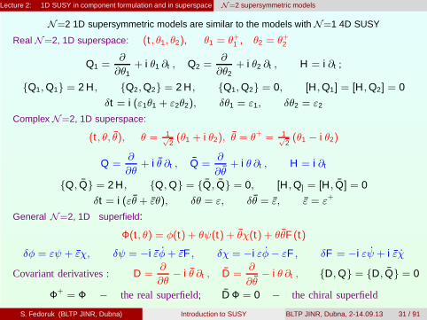
N -extended 1D superspace:

(t , θi), θk = (θk ), θi , θk = 0, i , j , k = 1, ...,N

Realization of super-Poincare algebra in superspace:

Qk = Q+k =

∂

∂θk+ i θk

∂

∂t, H = H+ = i ∂t ; Qk ,Qj = 2 δkj H , [H,Qk ] = 0

δt = εk Qk · t , δθk = εjQj · θk : δt = i εkθk , δθk = εk

General supersfield:

Φ(t , θk ) = φ(t)+ θkψk (t)+ θk1θk2φk1k2(t)+ θk1θk2θk3ψk1k2k3(t)+ · · ·+ θk1 . . . θkNφk1...kN (t)

Off-shell contents:

2N−1 bosonic(fermionic) component fieldsφ, φk1k2 , . . .

2N−1 fermionic(bosonic) component fieldsψk1 , ψk1k2k3 , . . .

if Φ(t , θk ) is bosonic(fermionic)

Covariant derivatives:

Dk =∂

∂θk− i θk

∂

∂t, Qj ,Dk = 0

F (Dk ) Φ = 0 − covariant constraint

On-shell (physical) contents of a model is defined by the action.


Lecture 2: 1D SUSY in component formulation and in superspace N=2 supersymmetric models

N=2 1D supersymmetric models are similar to the models with N=1 4D SUSY

Real N=2, 1D superspace: (t , θ1, θ2), θ1 = θ+1 , θ2 = θ+2

Q1 =∂

∂θ1+ i θ1 ∂t , Q2 =

∂

∂θ2+ i θ2 ∂t , H = i ∂t ;

Q1,Q1 = 2 H, Q2,Q2 = 2 H, Q1,Q2 = 0, [H,Q1] = [H,Q2] = 0

δt = i (ε1θ1 + ε2θ2), δθ1 = ε1, δθ2 = ε2

Complex N=2, 1D superspace:

(t , θ, θ), θ = 1√2(θ1 + i θ2), θ = θ+ = 1√

2(θ1 − i θ2)

Q =∂

∂θ+ i θ ∂t , Q =

∂

∂θ+ i θ ∂t , H = i ∂t

Q, Q = 2 H, Q,Q = Q, Q = 0, [H,Q] = [H, Q] = 0

δt = i (εθ + εθ), δθ = ε, δθ = ε, ε = ε+

General N=2, 1D superfield:

Φ(t , θ) = φ(t) + θψ(t) + θχ(t) + θθF (t)

δφ = εψ + εχ, δψ = −i εφ+ εF , δχ = −i εφ− εF , δF = −i εψ + i εχ

Covariant derivatives: D =∂

∂θ− i θ ∂t , D =

∂

∂θ− i θ ∂t , D,Q = D, Q = 0

Φ+ = Φ − the real superfield; D Φ = 0 − the chiral superfield



Real superfield:

Φ(t , θ) = Φ+ = φ(t) + θψ(t)− θψ(t) + θθF (t), φ+ = φ, F+ = F , ψ+ = ψ

Off-shell SUSY transformations:

δφ = εψ − εψ, δψ = −i εφ+ εF , δψ = i εφ+ εF , δF = −i (εψ + εψ)

S = i2

∫dt dθ d θ DΦDΦ= 1

2

∫dtφ2 + i (ψ ˙ψ − ψψ) + F 2

On− shell : φ = 0, ψ = 0, ˙ψ = 0, F = 0 (1, 2,1) multiplet

On-shell action:

S = 12

∫dtφ2 + i (ψ ˙ψ − ψψ)

On-shell SUSY transformations:

δφ = εψ − εψ, δψ = −i εφ, δψ = i εφ

[δ1, δ2]ψ = i (ε1ε2 − ε2ε1) ψ − 2i ε1ε2˙ψ︸︷︷︸

=0 on−shell

On-shell SUSY transformations are closed only on equations of motion.



Chiral superfield:

D Φ = 0 → Φ(t , θ) = φ(t) + θψ(t)− i θθφ(t), φ, ψ − complex fields

(2, 2, 0) multiplet

Φ(t , θ) = φ(t) + θψ(t)− i θθφ(t) = φ(tL) + θψ(tL) = Φ(tL, θ)

Chiral N=2, 1D subspace:(tL, θ), tL ≡ t − i θθ

δt = i (εθ + εθ), δθ = ε, δθ = ε ⇒ δtL = 2i εθ, δθ = ε

Supercharges in superspace (tL, θ, θ):

Q =∂

∂θ, Q =

∂

∂θ+ 2i θ ∂tL

SUSY transformations of component fields:

δφ = εψ , δψ = −2i εφ

SUSY invariant action:

S = − 12

∫dt dθ d θ DΦ DΦ = 1

2

∫dt

4φ ˙φ− i (ψ ˙ψ − ψψ)


Lecture 2: 1D SUSY in component formulation and in superspace (Super)conformal mechanics in black hole physics

In the near horizon limit the extreme (M = Q) Reissner-Nordström black hole solutionof Einstein-Maxwell equations are (in the units with G = 1)

ds2 = −( r

M

)2dt2 +

(Mr

)2

dr2 + M2dΩ

But −( r

M

)2dt2 +

(Mr

)2

dr2 = ηµνdxµdxν

where ηµν = diag(−,+,−), ηµνxµxν = −M2,x0 = (2r)−1[1 + r2(M2 − t2)], x1 = (2r)−1[1 − r2(M2 + t2)], x2 = Mrt .

The near horizon limit the extreme Reissner-Nordström black hole possessesAdS2 × S2 geometry.

AdS2 part, having SO(2, 1) symmetry, is described by conformal mechanics.

Superconformal mechanics models describe motion of the particle with angularmomentum (spin) near horizon of the extreme Reissner-Nordström black hole.


Lecture 2: 1D SUSY in component formulation and in superspace Conformal mechanics: peculiarities

Conformal mechanics action:

S = 12

∫dt(

x2 − gx2

)

Conformal invariance:

δt = a + b t + c t2 ≡ f (t), δx = 12 f x , δS =

∫dt Λ , Λ = 1

4 f x2

Conserved charges(

p = x ; ddt (H δt − p δx + Λ) = 0

):

H = 12

(p2 + g

x2

)

D = tH − 12 xp

K = t2H − txp + 12 x2

ddt

K =∂

∂tK + K ,HP = 0,

ddt

D =∂

∂tD + D,HP = 0, H − the Hamiltonian

H,DP = H, K ,DP = −K , H,KP = 2D − dynamical symmetry

[A,B] = iA,BP : [H,D] = i H, [K,D] = −i K, [H,K] = 2i D − sl(2,R) algebra


Lecture 2: 1D SUSY in component formulation and in superspace Conformal mechanics: peculiarities

Properties of the conformal mechanics:

If H |E >= E |E >, then H eiαD |E >= e2α E |E > ⇒the spectrum of H is continuous;

The eigenspectrum of H includes all E>0 values,for each of which there exists a plane wave narmalizable state;

The spectrum of H does not have an endpoint (ground state),the state with E=0 is not even plane wave normalizible.

It is obstacle to describe the conformal theory in terms of H eigenstates.

The sl(2,R) algebra in the Virasoro form:

R = 12 (a H +

1a

K), L± = − 12 (a H − 1

aK ∓ i D); a is a parameter

[R, L±] = ±L±, [L+,L−] = −2 RR is the u(1) generator in sl(2,R) ∼ o(1,2) algebra.

The eigenvalues of

R|t=0, a=1 = 12

(p2 +

gx2

+ x2)

are given by a discrete series

rn = r0 + n, n = 0, 1,2, . . . ; r0 = 12

(1 +

√g + 1

4

)


Lecture 2: 1D SUSY in component formulation and in superspace Black hole interpretation of conformal mechanics

The absence of a normalizable ground states in the conformal mechanics andnecessity to redefine the Hamiltonian are given in black hole interpretation.

In the black hole interpretation, eigenstates E of H describe the states with time-likeenergy-momentum vector, pµpµ > 0.

The absence of a ground state at E = 0 can be interpreted as impossibility to covernull geodesics of the event horizon with pµpµ = 0 by the static time coordinatesadapted by H.

Thus, the passing from H to “the Hamiltonian” R is transition to “good” time coordinatenear horizon.

Calogero model (multiparticle generalization of conformal mechanics)

S = 12

∫dt[ n∑

a=1

xaxa −∑

a 6=b

c2

(xa − xb)2

], H = 1

2

[ ∑

a

papa +∑

a 6=b

c2

(xa − xb)2

]

in the large n limit may provide the description of the extreme RN black holes in thenear horizon limit.


Lecture 2: 1D SUSY in component formulation and in superspace N= 2 superconformal mechanics

The N= 2 superconformal group OSp(2|2)∼SU(1,1|1)

Q, Q = 2H, S, S = 2K , Q, S = 2(D − U), S, Q = 2(D + U),

i[P,(

SS

)]= −

(QQ

), i

[K ,(

QQ

)]=

(SS

),

i[D,(

QQ

)]=

12

(QQ

), i

[D,(

SS

)]= −1

2

(SS

),

i[U,(

QQ

)]=

12

(Q

−Q

), i

[U,(

SS

)]= −1

2

(S

−S

)

The closure of S, S with Q, Q ⇒ the full OSp(2|2).We obtain the superconformal transformations by nonlinear realization method.

——————Coset realization of N = 2 superspace:

G = H,Q, Q,U, H = U, K = H,Q, Q

K(t , θ, θ) = eitH+θQ+θQ , t , θ, θ are the coordinates on the coset

eεQ+εQ eitH+θQ+θQ = eit′H+θ′Q+θ′Q : δt = i(εθ + εθ), δθ = ε, δθ = ε

Note : eA eB = exp

A + B + 12 [A,B] + 1

12 ([A, [A,B]] + [[A,B],B]) + · · ·


Lecture 2: 1D SUSY in component formulation and in superspace N= 2 superconformal mechanics

Coset realization of SU(1,1|1):

G = H,D,K ,Q, Q,S, S,U, H = U, K = H,D,K ,Q, Q,S, S

K = eitH eθQ+θQ eiuD eizK eζS+ζS

eεQ+εQ K = K′H, eηS+ηS K = K′HNote : eA B e−A = eA∧B, 1∧B ≡ B, A∧B ≡ [A,B], A2∧B ≡ [A, [A,B]], · · ·

δt = i(εθ + εθ), δθ = ε, δθ = ε;

δ′t = i(ηθ + ηθ)t , δ′θ = η(t − iθθ), δ′θ = η(t + iθθ)

δ′(dtd2θ) = 0, δ′D = −2i ηθD, δ′D = −2i ηθ D

——————

X = x(t) + θψ − θψ(t) + θθF (t), δ′X = i(ηθ + ηθ)X

S =

∫dtd2θ

(12 DXDX+ γ ln X

)= 1

2

∫dt

x2 + i (ψ ˙ψ − ψψ)− γ2 + γψψ

x2

Multi-particle generalization (N=2 superconformal Calogero):

S =

∫dt d2θ

1

2

∑

a

DXaDXa + γ∑

a 6=b

ln |Xa − Xb|


Lecture 2: 1D SUSY in component formulation and in superspace Brief sketch on N= 4 superconformal mechanics

The standard N=4, 1D superspace:

t , θk , θk = (θk )

+, k = 1,2

Supersymmetry transformations from the N= 4, 1D superconformal group D(2,1;α):

δt = i(θk εk − εk θ

k ), δθk = εk , δθk = εk ;

δ′t = −i(ηk θk − ηkθk )t + (1 + 2α)θj θ

j(ηk θk + ηkθk ),

δ′θk = ηk t − 2iαθkθj ηj + 2i(1 + α)θk θ

jηj − i(1 + 2α)ηkθj θj

Covariant derivatives: Dk =∂

∂θk+ i θk∂t Dk =

∂

∂θk+ i θk∂t

Some types of the N=4, 1D superfields:

Dk DkX = m, Dk DkX = m, [Dk , Dk ]X = 0 - scalar superfield, (1,4,3) multiplet

D(iV jk) = 0, D(iV jk) = 0 - vector superfield, (3,4,1)

Superconformal models (X = (V ik Vik )1/2 for vector superfield):

S ∼∫

dt d4θ X−1/2 for α 6= −1; S ∼

∫dt d4θ X lnX for α = −1

In components: S ∼∫

dt[x2 + i (ψk

˙ψk − ψk ψk )− g + F (ψ, ψ)

x2

]

More general formulations of N=4, 1D models is achieved in harmonic superspace


Lecture 3: 4D SUSY in superspace

Lecture 3: 4D SUSY in superspace

N = 1 4D superspace.

N = 1 4D superfields action.

N -extended SUSY in superspace.

N = 2 4D in harmonic superspace formulation.

Superstring action.


Lecture 3: 4D SUSY in superspace N = 1 4D superspace

The Poincaré group has a natural realization in the Minkowski space

M(4) = (xµ) , µ = 0, 1, 2, 3

We can consider the Minkowski space as the coset

M(4) =Poincare groupLorentz group

= (Pµ, Lµν) / (Lµν) .

k(xµ) = expixµPµ , g(εµ, εµν) · k(xµ) = k(x ′µ) · ℓ(xµ, εµ, εµν)

The Poincaré supergroup can be realized in the coset

M(4|4) =Poincare supergroup

Lorentz group=(Pµ, Lµν ,Qα, Qα

)/ (Lµν) .

Exponential parametrization of it:

k(xµ, θα, θα) = exp

ixµPµ + iθαQα − i θαQα

,

where new spinor coordinates θα, θα of coset are anticommuting parameters.



The extended manifold

M(4|4) =(

xµ , θα , θα),

is called N = 1 Minkowski superspace.

The spinor coordinates are called odd or Grassmann coordinates and have theGrassmann parity −1, while xm are even coordinates having the Grassmann parity +1

[θα, xµ] = [θα, xµ] = 0 , θα, θβ = θα, θβ = 0 .

Important consequence: fermionic coordinates are nilpotent, θ1θ1 = θ2θ2 = 0 .

From (ǫα, ǫα are anticommuting parameters and spinor coordinates also anticommutewith them)

exp

iεαQα − i εαQα

exp

ixµPµ + iθαQα − i θαQα

= exp

ix ′µPµ + iθ′αQα − i θ′αQα

we obtain supersymmetry transformations on superspace

θα′ = θα + εα , θα′ = θα + εα .

xµ′ = xµ − i(ǫσmθ − θσm ǫ) .

Supersymmetry transformations are realized as translations in nilpotent directions ofthe superspace.



The general scalar N = 1 superfield

Φ′(x ′, θ′, θ′) = Φ(x , θ, θ) .

has the following finite series expansion in Grassmann coordinates

Φ(x , θ, θ) = φ(x) + θα ψα(x) + θα χα(x) + θ2 M(x) + θ2 N(x)

+ θσµθ Aµ(x) + θ2 θα ρα(x) + θ2 θα λα(x) + θ2 θ2 D(x) ,

where θ2 := θαθα = ǫαβθαθβ , θ2 = θαθ

α = ǫαβ θβ θα , ǫ12 = ǫ12 = 1.

Here there are 8 bosonic and 8 fermionic independent complex component fields.

The reality condition

(Φ) = Φ

implies the following reality conditions for the component fields

φ(x) = φ(x) , χα(x) = ψα(x) , M(x) = N(x) , Aµ(x) = Aµ(x) ,

λα(x) = ρα(x) , D(x) = D(x) .

They leave in Φ just (8 + 8) independent real components.



The transformation law Φ′(x , θ, θ) = Φ(x − δx , θ − ǫ, θ − ǫ) implies

δΦ = −ǫα ∂Φ∂θα

− ǫα∂Φ

∂θα− δxm ∂Φ

∂xm≡ i(ǫαQα + ǫαQα

)Φ

and leads to the expressions for supercharges

Qα = i∂

∂θα+ θα(σµ)αα

∂

∂xµ, Qα = −i

∂

∂θα− θα(σµ)αα

∂

∂xµ,

Qα, Qα = 2Pµ , Qα,Qβ = Qα, Qβ = 0 , Pµ = −i∂

∂xµ.

The relevant transformations of component fields are obtained from the formula

δΦ = δφ+ θαδψα + . . .+ θ2θ2δD

and are

δφ = −ǫψ − ǫχ , δψα = −i(σmǫ)α∂mφ− 2ǫαM − (σmǫ)αAm , . . . ,

δD =i2∂mρσ

mǫ − i2ǫσm∂mλ .

The supermultiplet of fields encompassed by Φ(x , θ, θ) is reducible.How to describe irreducible supermultiplets in the superfield language?



An important element of the superspace formalism are spinor covariant derivatives

Dα =∂

∂θα+ i θα(σµ)αα

∂

∂xµ, Dα = − ∂

∂θα− iθα(σµ)αα

∂

∂xµ,

Dα, Dα = −2i(σm)αα∂m , Dα,Dβ = Dα, Dβ = 0 .

The covariant derivatives anticommute with supercharges,

D,Q = D, Q = 0,

so DαΦ and DαΦ are again superfields:

δDαΦ = DαδΦ = Dαi(ǫαQα + ǫαQα

)Φ = i

(ǫαQα + ǫαQα

)DαΦ .

With the help of the covariant spinor derivatives it becomes possible to definesuperfield description of the irreducible supermultiplets.



Chiral superfieldsChirality condition

DαΦL(x , θ, θ) = 0

impliesΦL(x , θ, θ) = ϕL(xL, θ) = φ(xL) + θαψα(xL) + θθF (xL) ,

wherexm

L = xm + iθσmθ .

We obtain less independent fields: the set φ, ψα,F is closed under N = 1supersymmetry:

δφ = −ǫψ , δψα = −2i(σmǫ)α∂mφ− 2ǫαF , δF = −i ǫσm∂mψ .

This is just the transformation law of the scalar N = 1 supermultiplet.

The geometric interpretation: the subspace (chiral N = 1 superspace)

(xmL , θ

α)

is closed under N = 1 supersymmetry:

δxmL = 2iθσmǫ , δθα = ǫα .

In the basis (xmL , θ

α, θα): Dα =∂

∂θα.


Lecture 3: 4D SUSY in superspace Superfield actions

Scalar superfield Lagrangian:

L = L(Φ,DαΦ, DαΦ, ∂mΦ, . . .) , δL = i(ǫαQα + ǫαQα

)L .

The variation of the higher component of any expansion of any superfield is atotal derivative. This component is extracted by the Berezin integral. It isequivalent to differentiation in Grassmann coordinates. In the considered case ofN = 1 superspace it is defined by the rules∫

d2θ (θ)2 = 1 ,∫

d2θ (θ)2 = 1 ,∫

d2θd2θ (θ)4 = 1 , (θ)4 ≡ (θ)2(θ)2

Invariant superfield action:

S =

∫d4xd4θL(Φ,DαΦ, DαΦ, ∂mΦ, . . .) , δL = i

(ǫαQα + ǫαQα

)L .



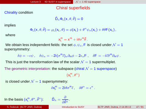
Chiral superfieldThe kinetic terms is as follows

Skin =

∫d4xd4θΦ(xL, θ)Φ(xR , θ) , xµ

R = (xµL ) = xµ − iθσµθ .

After performing integration over Grassmann coordinates, one obtains

S ∼∫

d4x(∂µφ∂µφ− i

2ψσµ∂µψ + FF

).

The total Wess-Zumino model action is reproduced by adding, to this kinetic term,also potential superfield term

Spot =

∫d4xLd2θ

(g3Φ3 +

m2Φ2)+ c.c. .

This action is the only renormalizble action of the scalar N = 1 multiplet. In principle,one can construct more general actions, e.g., the action of Kähler sigma model andgeneralized potential term

Skin =

∫d4xd4θ K

[Φ(xL, θ), Φ(xR , θ)

], Spot =

∫d4xLd2θ P(Φ) + c.c. .



Vector superfield (N = 1 SYM)It is described by the real superfield V (x , θ, θ) possessing the gauge freedom

δV (x , θ, θ) = i[λ(xµ − iθσµθ, θ)− λ(xµ + iθσµθ, θ)],

where λ(xL, θ) is an arbitatry chiral superfild parameter. Using this freedom, one canchoose the so called Wess-Zumino gauge

VWZ (x , θ, θ) = 2 θσµθ Aµ(x) + 2i θ2θα ψα(x)− 2iθ2θα ψα(x) + θ2θ2 D(x) .

Residual gauge invariance in WZ gauge: A′µ(x) = Aµ + ∂µλ(x).

The invariant action is written as an integral over the chiral superspace

SN=1gauge =

116

∫d4xLd2θ (WαWα) + c.c. ,

where Wα = −12

D2DαV is chiral DαWα = 0 .

The corresponding component off-shell action reads (Fµν = ∂µAν − ∂νAµ)

S =

∫d4x

[−1

4FµνFµν − iψσµ∂µψ +

12

D2].



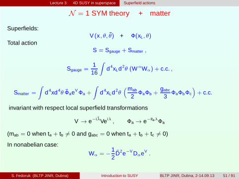
N = 1 SYM theory + matter

Superfields:V (x , θ, θ) + Φ(xL, θ)

Total actionS = Sgauge + Smatter ,

Sgauge =1

16

∫d4xLd2θ (WαWα) + c.c. ,

Smatter =

∫d4xd4θ ΦaeVΦa +

∫d4xLd2θ

(mab

2ΦaΦb +

gabc

3ΦaΦbΦc

)+ c.c.

invariant with respect local superfield transformations

V → e−iλVeiλ , Φa → e−itaλΦa

(mab = 0 when ta + tb 6= 0 and gabc = 0 when ta + tb + tc 6= 0)

In nonabelian case:

Wα = −12

D2e−V DαeV .


Lecture 3: 4D SUSY in superspace N -extended SUSY in superspace

The difficulties in case of higher N supersymmetries arise because the relevantsuperspaces contain too many θ coordinates and many component fields,

2n for n Grassmann coordinates ,

and it is a very complicated constraints to define the superfields which would correctlydescribe the relevant irreps.

Let us consider N = 2 case.

N=2, 4D SUSY algebra:

Pµ, Qkα, Qαk = (Qk

α)+, Lµν ,

R−symmetry︷︸︸︷J(ik),︸︷︷︸su(2)

, i , k = 1,2

StandardN= 2, 4D superspace:

Pµ, Qkα, Qαk , Lµν , J ik

/

Lµν , J ik

Standard superspace coordinates:

xµ, θαk , θαk = (θαk )

+

Basic N = 2 superfield (hypermultiplet superfield) q j(x , θ, θ) subjected by theconstraints

D(iα q j)(x , θ, θ) = 0 , D(i

α q j)(x , θ, θ) = 0

does not have off-shell description (Lagrangian description) in standard superspace. Itpossesses an off-shell formulation only in the N = 2 harmonic superspace.


Lecture 3: 4D SUSY in superspace Harmonic superspace for N= 2, 4D SUSY models

suL(2) algebra: J(ik) =

J±, J 0, J 0 − u(1) generator

N= 4, 1D harmonic superspace:

Pµ, Qkα, Qαk , Lµν , J ik

/

Lµν , J 0

Harmonic superspace coordinates:

xµ, θαk , θαk , u±

i

Harmonic coordinates parametrize S 2 ∼ SU(2)/U(1) by two SU(2) spinors

u±i , u−

i = (u+i)

which subject to the constraint u+i u−i = 1 → u+

i u−k − u+

k u−i = ǫik

and are defined up to a U(1) phase transformations

u+i → eiαu+

i , u−i → e−iαu−

i

||u|| =(

u+1 u−

1u+

2 u−2

)∈ SU(2), ||u|| → g ||u|| h , g ∈ SU(2), h ∈ U(1)

Any function on S 2 ∼ SU(2)/U(1) must have a definite U(1) charge q

Φ(q)(u) =∞∑

n=0

φi1...i n+q j1...j n u+i1. . . u+

i n+qu−

j1. . . u−

j nfor n ≥ 0

Harmonic functions are defined up to the transformations Φ(q) → eiαqΦ(q).

The use of such parametrization of S 2 has the advantage of manifest SU(2) covarianceS. Fedoruk (BLTP JINR, Dubna) Introduction to SUSY BLTP JINR, Dubna, 2-14.09.13 53 / 91


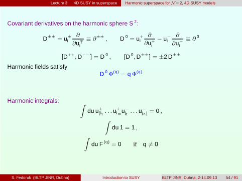
Covariant derivatives on the harmonic sphere S 2:

D±± = u±i

∂

∂u∓i

≡ ∂±± , D 0 = u+i

∂

∂u+i

− u−i

∂

∂u−i

≡ ∂ 0

[D++,D−−] = D 0 , [D 0,D±±] = ±2 D±±

Harmonic fields satisfyD 0 Φ(q) = q Φ(q)

Harmonic integrals: ∫du u+

(i1. . . u+

i mu−

j1. . . u−

j n)= 0 ,

∫du 1 = 1 ,

∫du F (q) = 0 if q 6= 0



Central basis in harmonic superspace:

xµ, θαk , θαk , u±

i

≡ z, u

The N= 4, 1D Poincare supersymmetry:

δxµ = i(εkσµθk − θkσµεk ), δθαk = εαk , δθαk = εαk , δu±i = 0

Analytic basis in harmonic superspace:

xµA , θ

±α , θ

±α , u

±i

≡ zA, u ,

where θ±α = θiαu±

i , θ±α = θiαu±

i , xµA = xµ − i

(θ+σµθ− + θ−σµθ+

)

Analytic superspace (with half odd coordinates)

xµA , θ

+α , θ

+α , u

±i

≡ ζ, u

is closed under N= 4 Poincare SUSY (and under N= 4 superconformal symmetry)

δxµA = −2i(εkσµθ+ + θ+σµεk )u−

k , δθ+α = εiαu+

i , δθ+α = εiαu+

i , δu±i = 0


Lecture 3: 4D SUSY in superspace Harmonic superfield models

Covariant derivatives D±α = Di

αu±i , D±

α = Diαu±

i in analytic basis:

D+α =

∂

∂θ−α, D+

α = − ∂

∂θ−α, D−

α =∂

∂θ+α−2i(σµθ

−)α∂µA , D−

α =∂

∂θ+α+2i(θ−σµ)α∂

µA

Therefore,D+

α Ψ(z, u) = D+α Ψ(z, u) = 0 ⇒ Ψ = Ψ(ζ, u)

– superfield that lives on the analytic superspace depends on half of the Grassmannvariables and has a smaller number of component fields.

HypermultipletIt is described by the analytic superfield q+, D+q+ = D+q+ = 0

Invariant (free) action:

S =

∫dζAdu q+D++q+

Analytic basis:D++q+ = 0 ⇒ equations of motion

Central basis:

D++q+ = 0 ⇒ q+ = q i(z)u+i

D+q+ = D+q+ = 0 ⇒ D(i qk) = D(iqk) = 0 (resolution of the constraints)

Self-interactions:

Sint =

∫dζAdu

[a(q+)4 + b(q+q+)2 + (q+)4

]


Lecture 3: 4D SUSY in superspace Superstring action

Fermionic string (Neveu-Schwarz-Ramond string) – 2d world-sheet supersymmetrySuperstring (Green-Schwarz superstring) – D = 3, 4, 6, 10 target space

supersymmetry

σα = (σ1, σ2) − world-sheet coordinates, γα = eαa γ

a, α = 1,2

Xµ(σ), ΘA(σ) − target-space 2 fields, µ = 0, 1, ...,D − 1, A = 1, ..., 2D2

Target-space supersymmetry:

δΘA = εA, δXµ = i εΓµΘ,

where Γµ are Dirac matrices in D-dimensional space-time.SUSY invariant one-forms

ωµ = dXµ − iΘΓµdΘ, ωµ ≡ dσαωµ,α

N = 1 GS superstring action SGS =∫

d2σLGS,

LGS = T(√

ggαβ ωµ,αωµ,β + 2ǫαβ∂αXµ ΘΓµ∂βΘ

)

Quantum spectrum of the superstring contains infinite towers of states havinghigher spins

(SYM on ground state or SUGRA on ground state of N = 2 GS superstring).

Higher spin fields will be considered in the lessons by M.Vasiliev and V.Didenko.


Lectures 4,5: The elements of twistor theory


Symmetries of massless particle action.

Twistor space and its geometry.

Twistor transform.

Supertwistors.

(Super)twistors in HS theory and superstring theory.



Proposed in 1967 by R. Penrose the twistor theory provides a basis for a newmathematical tool in theoretical physics, in which the complex structure of quantumfield theory would follow directly from the complex structure of the new base space(replacing the usual space-time).

Although there is still no consensus on the interpretation of the twistor theory,or as a more suitable base (instead of the space-time approach) to build a futurecomplete theory of fundamental interactions,or as a powerful mathematical tool for analyzing the conventional theories,the twistor methods are very popular in modern theoretical physics.

Twistor methods allowed to develop new methods of constructing solutions of theEinstein equations, have led to some progress in the construction of quantum gravity,yielded non-trivial results in the Yang-Mills theory.

Twistor theory is used extensively in the theory of monopoles and instantons and inthe analysis of higher spin theory and superstring theory.

The ground positions of the twistor theory is best explored when analyzing masslessparticle and its quantization.


Lectures 4,5: The elements of twistor theory Symmetries of massless particle action

The action of the relativistic spinless particles in the first-order formalism

S1 =

∫dτ(

pµxµ − e(p2 − m2)).

xµ(τ ), pµ(τ ) are the position and momentum variables; their Poisson brackets are[xµ, pν ]P = δµν . τ is evolution parameter. e(τ ) is Lagrange multiplier for the constraint

p2 − m2 ≈ 0 ,

determining the mass of the particle.

Inserting equations of motion pµ = xµ/(2e) back in S1 we obtain the action in thesecond-order formalism

S2 =12

∫dτ(

xµxµ

e+ em2

).

It is 1D gravity-like action where e(τ ) plays the role of 1D gravity field and secondterm is 1D analog of 4D term with cosmological constant.

Insertion of equation of motion e =√

xµxµ/m back in S2 yields the square-rootaction

S = m∫

dτ√

xµxµ .

The last action is only valid for a massive particle with m 6= 0.



Let us consider massless case m = 0.The action S1 is invariant with respect the following global transformations

δxµ = aµ + lµνxν + cxµ + 2(k · x)xµ − x2kµ , δe = 2ce + 4(k · x)e ,

δpµ = lµνpν − cpµ + 2(k · p)xµ − 2(k · x)pµ − 2(x · p)kµ .

Generators of these transformations (conserved charges)

Pµ = pµ , Lµν = xµpν − xνpµ , D = xµpµ , Kµ = 2(x · p)xµ − x2pµ

form conformal algebra (here we will take ηµλ = diag(−+++)) with respect thePoisson brackets [xµ, pν ]P = δµν :

[Lµν , Lλσ]P = ηµλLνσ − ηµσLνλ − (µ↔ ν) ,

[Lµν ,Pλ]P = ηµλPν − (µ↔ ν) , [Lµν ,Kλ]P = ηµλKν − (µ↔ ν) ,

[Pµ,D]P = −Pµ , [Kµ,D]P = Kµ , [Pµ,Kν ]P = 2Mµν − 2ηµνD .

Conformal boosts are non-linear transformations in the space-time. In space-timeformulation it is a hidden symmetry of conformally invariant systems. For example, inthe case of conformal transformations we have δ = −4(kx)+ 4kµ∂µ, ≡ ∂µ∂µ.Therefore, the conformal invariance of the simplest Klein-Gordon equation Φ(x) = 0assumes the following transformations of massless scalar field δΦ = −2(kx)Φ.



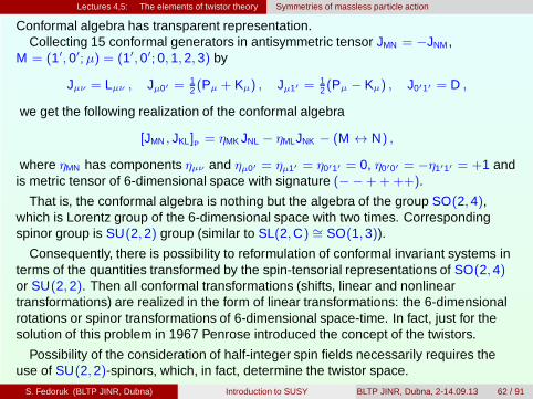
Conformal algebra has transparent representation.Collecting 15 conformal generators in antisymmetric tensor JMN = −JNM ,

M = (1′, 0′;µ) = (1′, 0′; 0, 1,2, 3) by

Jµν = Lµν , Jµ0′ =12 (Pµ + Kµ) , Jµ1′ =

12 (Pµ − Kµ) , J0′1′ = D ,

we get the following realization of the conformal algebra

[JMN , JKL]P = ηMK JNL − ηMLJNK − (M ↔ N) ,

where ηMN has components ηµν and ηµ0′ = ηµ1′ = η0′1′ = 0, η0′0′ = −η1′1′ = +1 andis metric tensor of 6-dimensional space with signature (−−++++).

That is, the conformal algebra is nothing but the algebra of the group SO(2,4),which is Lorentz group of the 6-dimensional space with two times. Correspondingspinor group is SU(2,2) group (similar to SL(2,C) ∼= SO(1,3)).

Consequently, there is possibility to reformulation of conformal invariant systems interms of the quantities transformed by the spin-tensorial representations of SO(2,4)or SU(2,2). Then all conformal transformations (shifts, linear and nonlineartransformations) are realized in the form of linear transformations: the 6-dimensionalrotations or spinor transformations of 6-dimensional space-time. In fact, just for thesolution of this problem in 1967 Penrose introduced the concept of the twistors.

Possibility of the consideration of half-integer spin fields necessarily requires theuse of SU(2,2)-spinors, which, in fact, determine the twistor space.


Lectures 4,5: The elements of twistor theory Twistor space

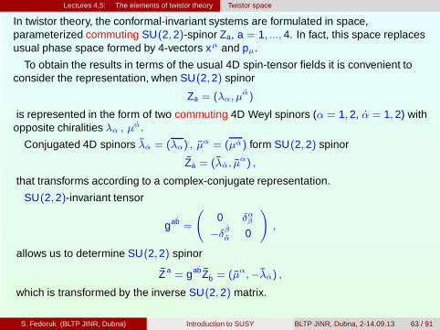
In twistor theory, the conformal-invariant systems are formulated in space,parameterized commuting SU(2,2)-spinor Za, a = 1, ..., 4. In fact, this space replacesusual phase space formed by 4-vectors xµ and pµ.

To obtain the results in terms of the usual 4D spin-tensor fields it is convenient toconsider the representation, when SU(2,2) spinor

Za = (λα, µα)

is represented in the form of two commuting 4D Weyl spinors (α = 1,2, α = 1, 2) withopposite chiralities λα , µ

α.

Conjugated 4D spinors λα = (λα) , µα = (µα) form SU(2,2) spinor

Za = (λα, µα) ,

that transforms according to a complex-conjugate representation.

SU(2,2)-invariant tensor

gab =

(0 δαβ

−δβα 0

),

allows us to determine SU(2,2) spinor

Z a = gabZb = (µα,−λα) ,

which is transformed by the inverse SU(2,2) matrix.



The contraction of the spinor Za and its adjoint Z a defines a Hermitian form

Λ ≡ i2 Z aZa = i

2 gabZbZa = i2 (µαλα − λαµ

α)

which is SU(2,2)-invariant and defines the norm of SU(2,2) spinor Za.

The twistor space T is a spinor space (the space C4) conformal group SU(2,2) withHermitian form Λ.

The twistors are SU(2,2) spinors Za, defined on the twistor space.

Depending on the value of the Hermitian form Λ, there are the following subsets of thetwistor space:

the positive twistor space T+, where Λ > 0,

the negative twistor space T−, where Λ < 0

the isotropic twistor space T0, where Λ = 0.

We will see below that the twistor norm Λ defines the helicity of massless particle.



From the definition, conformal transformations are realized by linear transformationson the twistor space. The infinitesimal transformations of spinor components are

δλα = lαβλβ − 1

2 c λα − kαβµβ ,

δµα = l αβµβ + 12 c µα + aαβλβ .

Defining the Poisson brackets in the twistor space

[Z a,Zb]P = δab : [µα, λβ]P = δαβ , [µα, λβ]P = δαβ ,

we find that these transformation are generated by the following quantities

Pαα = λαλα , K αα = µαµα ,

Lαβ = λ(αµβ) , Lαβ = λ(αµβ) ,

D = 12 (µ

αλα + λαµα) .

They form the conformal algebra and leave invariant the twistor norm. In terms of the4-component twistor formalizm, these generators are presented in the form of atraceless product of twistor Za and its adjoint Z a:

Z aZb − 14 δ

ab Z cZc .


Lectures 4,5: The elements of twistor theory Two-spinor notations

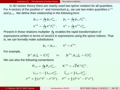
In 4D twistor theory there are mainly used two-spinor notation for all quantities.For 4-vectors of the position xµ and momentum pµ we use two-index quantities x αα

and pαα. We define their relationship in the following form

pαα = 1√2

pµσµαα , pµ = 1√

2pαασ

ααµ ,

x αα = 1√2

xµσααµ , xµ = 1√

2x αασµ

αα .

Present in these relations multiplier 1√2

enables the rapid transformation ofexpressions written in terms of vectors in expressions using the spinor indices. Thatis, we can formally make substitutions

pµ = pαα , xµ = x αα .

For example,[xµ, pν ]P = δµν δ

αβ ⇔ [x αα, pββ]P = δαβ δ

αβ .

We use also the following conventions

Pαα = 1√2

Pµσµαα , K αα =

√2 Kµσαα

µ ,

Lαβ = − 12 Lµνσ

µναβ , Lαβ = 1

2 Lµν σµν

αβ,

σµν = 14 (σµσν − σν σµ) , σµν = 1

4 (σµσν − σνσµ) .


Lectures 4,5: The elements of twistor theory Twistor transform

That is, we have two formalism to describe the conformal-invariant systems:space-time description and twistor formulation.

The relationship of space-time and twistor variables is defined by the relations

pαα = λαλα ,

µα = x αβλβ , µα = λβx βα .

These relations are the Penrose twistor transform for the coordinates.

When twistor transform are valid, then

twistor representation of conformal generators goes into space-time realizationof them;

conformal transformations of twistor variables yield conformal transformations ofspace-time quantities.

space-time and twistor symplectic structures are compatible with one another:the Poisson brackets of any two quantities equal to each other when using thespace-time Poisson brackets or twistor Poisson brackets.



The relations of twistor transform have clear physical and geometrical meaning.

Equations pαα = λαλα automatically mean light-like 4-momentum of the particlep2 = 0. This follows directly from the identity λαλα = ǫαβλβλα ≡ 0, which is valid forcommuting 4D spinors.

The conditions µα = x αβλβ , µα = λβx βα establish the links between Minkowskispace-time and twistor variables. Its are the incidence conditions. In particular, for afixed twistors the solution for x

x αα = x αα0 + aλαλα

contains an arbitrary real constant a, parametrizing light-like line in Minkowski spacewith direction vector λαλα.

That is, (several) point of the twistor space correspond to light-like line in Minkowski

space.



Incidence conditions µα = x αβλβ , µα = λβx βα have important consequence: thetwistor, appearing in them, is isotropic

Λ = i2 Z aZa = i

2 (µαλα − λαµ

α) = 0 .

This is achieved, in fact, because the matrix x αα is Hermitian.

What is the isotropic twistor condition or, indeed, what is the physical meaning of thetwistor norm?

The answer to this question is found after the calculation of the Pauli-Lubanski vector

Wµ = 12 εµνλρPνMλρ .

In twistor realization of the generators we get

Wαα = ΛPαα ,

where Λ is the twistor norm and is defined above.

Thus, the twistor norm coincides with the helicity of massless particle, which isdescribed by this twistor.


Lectures 4,5: The elements of twistor theory Twistor action of massless spinless particle

The twistor action of massless spinless particle has the following form

Stwistor0 = 1

2

∫dτ[Z aZa − ˙Z aZa − il Z aZa

],

where l(τ ) is Lagrange multiplier for the constraint Λ = i2 Z aZa ≈ 0 (vanishing

helicity). Up to a total derivative, this action takes the following form in the 4D spinornotation

Stwistor0 =

∫dτ[˙µαλα + λαµ

α − i2 l(µαλα − λαµ

α)].

It should be noted that, up to a total derivative the kinetic term ˙µαλα + λαµα of this

action takes the form of the space-time kinetic term pµxµ after using the twistortransform.

Let us do the quantization of twistor particle: find twistor wave function and compare itwith the scalar field obtained in the space-time formulation.


Lectures 4,5: The elements of twistor theory Field twistor transform

At the transition to the quantum theory, the Poisson brackets go to the commutators

[ ˆZ a, Zb] = iδab .

The quantization of the twistor particles is conveniently carried out in the holomorphic

representation (the Penrose representation), where the operators Za diagonal, and ˆZ a

are realized as differential operators

ˆZ a = i∂

∂Za; ˆλα = −i

∂

∂µα, ˆµα = i

∂

∂λα.



Twistor wave functionΨ(Z ) = Ψ(λ, µ)

satisfies the equationΛΨ(Z ) = 0 .

Taking Weyl ordering in the helicity operator

Λ = i2 Z aZa → Λ = i

4 ( ˆZ aZa + ZaˆZ a) = i

2 ZaˆZ a − 1 = − 1

2 Za∂

∂Za− 1 ,

we find that the twistor wave equation has the form

12 Za

∂

∂ZaΨ = −Ψ ; 1

2 (λα∂

∂λα+ µα ∂

∂µα)Ψ = −Ψ .

Thus, the twistor wave function of the considered system is a holomorphichomogeneous function of homogeneity degree (−2):

Ψ(−2)(cZ ) = c−2Ψ(−2)(Z ) ,

where c is arbitrary complex number.



Usual space-time field is obtained from the twistor field by the Penrose twistortransform for the fields. It is constructed as follows. In the twistor field the spinor µ isresolved by the incidence conditions

Ψ(−2)(Z )∣∣∣µα=xααλα

= Ψ(−2)(λα, xααλα) .

Due to the homogeneity, this function is defined on the complex projective space CP1

and efficiently depends on a single complex variable. For example, it depends onz ≡ λ1/λ2 at λ2 6= 0. Integrating the twistor field with respect to this variable, we getthe usual space-time field. In the covariant record that does not depend on the choiceof independent coordinates on CP1, the twistor field is integrated with the measuredλ ≡ λαdλα

Φ(x) =∮λdλΨ(−2)(λα, x

ααλα) ,

where the integrand is invariant under λ→ cλ. In this integral transformation theintegration is performed along a closed loop in the space of independent complexvariable, covering the pole of the twistor field.

Defined integral transformation is the Penrose twistor transform for scalar field.

It is important that the field Φ(x) automatically satisfies massless Klein-Gordonequation ∂µ∂µΦ(x). This is the result of depending the twistor field on x αα only incombination x ααλα with commuting spinor λα, for which the identity λαλα ≡ 0 is valid.


Lectures 4,5: The elements of twistor theory Mixed wistor-space-time formulation

We have considered both purely space-time formulation of massless particle with zerohelicity or its purely twistor formulation.

There is also mixed formulation that uses both space-time and twistor variables.This is so-called Shirafuji twistor formulation.

The action of the massless spin-zero particles in the Shirafuji formulation is, in fact,space-time action, in which the momentum is resolved through the twistor variables

S0(mix) =

∫dτλαλαx αα .

That is, the importance of twistor relation

pαα − λαλα ≈ 0 .

is coded directly in mixed action.


Lectures 4,5: The elements of twistor theory Twistor transform as bridge

L = ˙µαλα + λαµα − i

2 l(µαλα − λαµα)

twistor formulation

µα = x αβλβ , µα = λβx βα

pαα = λαλα

Penrose transform

L = pααx αα − ep2

formulationspace-time

L = λαλαx αα

mixed formulation

6

?

-


Lectures 4,5: The elements of twistor theory Twistor transform as bridge

(Za

∂∂Za

+ 2)Ψ(−2)(Z ) = 0

Ψ(−2)(Z ) = Ψ(−2)(λα, µα)

twistor field

Φ(x) = 0

Φ(x) =∮λdλΨ(−2)(Z )|µα=xααλα

space-time field

-


Lectures 4,5: The elements of twistor theory Twistor formulation of massless spinning particle

In the twistor formulation of the helicity of the particles is determined by the twistornorm. Consequently, the phase space of massless particle of helicity s has to belimited to the constraint

Λ− s = i2 Z aZa − s = i

2 (µαλα − λαµ

α)− s ≈ 0 .

The action

Stwistors =

∫dτ[

12 (Z

aZa − ˙Z aZa)− l ( i2 Z aZa − s)

],

determines the twistor formulation of a massless particle nonzero helicity s.

Quantization of the system is carried out by analogy with the spinless case. Twistorconstraint yields the equation for the twistor wave function

12 Za

∂

∂ZaΨ = −(1 + s)Ψ .

Thus, the twistor field of massless particle with helicity s is holomorphichomogeneous function of degree (−2 − 2s)

Ψ(−2−2s)(Z ) .


Lectures 4,5: The elements of twistor theory Twistor formulation of massless spinning particle

Corresponding usual space-time field can be obtained by using the incidenceconditions and the Penrose field transform:

Φα1...α2s (x) =∮

(λdλ)λα1 . . . λα2sΨ(−2−2s)(λα, x

ααλα) .

In contrast to the zero-helicity case, here integrand contains 2s components of thespinor λ to compensate the negative weight of the twistor field.

The resulting space-time field is symmetric with respect to spinor indices because ofcommuting twistor component, Φα1...α2s = Φ(α1...α2s), and automatically satisfies theDirac equation

∂αα1Φα1...α2s (x) = 0 .

That is, it is complex self-dual field strength of massless particle of helicity s.


Lectures 4,5: The elements of twistor theory Massive particle in twistor formulation

If the massless case the light-like momentum vector is resolved in term of singlespinor, spinor representation of the time-like momentum of a massive particle

p2 = m2

must use at least two spinors (here it is summation with respect of repeating indexi = 1, 2)

pαα = λiα λα i ,

where λα i = (λiα).

Interpreting, by analogy with the massless case, the spinor λ as half the twistor,we find that a massive particle should have bitwistor description. Furthermore, twospinor used should be limited additional constraint

|λαiλαi |2 = m2

or perhaps stronger conditions, such as

λαiλαi = m , λαi λαi = m ,

which would violate the conformal symmetry to the Poincare group.


Lectures 4,5: The elements of twistor theory Massless superparticle

Superparticle action in the formalism of the first order is given by

Ssuper0 =

∫dτ(

pααωαα − epααpαα

), ωαα ≡ x αα − i θαθα + i ˙θαθα .

The action is invariant under the following global transformations:

Poincare transformations

δx αα = aαα + x αβ lβα + l αβx βα , δθα = θβ lβ

α ;

dilatationsδx αα = cx αα , δθα = 1

2 cθα ;

conformal boosts

δx αα = x αβkββx βα − 4θαθα θβkββ θβ , δθα = θβkββ(x

βα + i θβθα) ;

supertranslations

δx αα = −(θαǫα − ǫαθα) , δθα = ǫα ;

superconformal boosts

δx αα = 2i(θαηβx βα − x αβηβθα)− 4θαθα(θβηβ + ηβ θ

β) ,

δθα = −4iθα θβηβ + ηβ(xβα + i θβθα) ,

and chiral spinor transformations δθα = − 52 iφθα.

These nonlinear transformations form superconformal group SU(2,2|1).S. Fedoruk (BLTP JINR, Dubna) Introduction to SUSY BLTP JINR, Dubna, 2-14.09.13 80 / 91

Lectures 4,5: The elements of twistor theory Supertwistors

Supertwistor formulation solves the basic task: superconformal symmetry in it isrealized by linear transformations.

By analogy with the purely bosonic case, supertwistors defined as spinors of thesuperconformal group SU(2,2|1). Among the five components supertwistors

ZA = (Za; χ) = (λα, µα; χ) , A = 1, . . . , 5

four ones are c-numerical components, formed by usual twistor - SU(2,2)-spinor Za.Fifth component is Grassmann, complex Lorentz scalar χ , χ = (χ) .Conjugated supertwistor

ZA = (Z a; 2iχ) = (µα,−λα; 2iχ)

can be represented by complex-conjugated supertwistor

ZA = GABZB , ZB = (λα, µα; χ) ,

and SU(2,2|1)-invariant tensor

GAB =

(gab 00 2i

),

where gab is SU(2,2)-invariant tensor.SU(2,2|1)-invariant supertwistor norm is defined by

N ≡ i2 ZAZA = i

2 GABZBZA = i2 (µ

αλα − λαµα)− χχ .



Conformal transformations act only on bosonic components of the supertwistor andare defined previously. Supertranslations and superconformal boosts, realized linearlyon the supertwistor space, mix bosonic and fermionic components of thesupertwistors

δλα = 2iηαχ , δµα = 2i ǫαχ , δχ = ǫαλα − ηαµα .

Chiral transformations of supertwistor components are

δλα = i2 φλα , δµα = i

2 φµα , δχ = iφχ .

Introducing the (graded) symplectic structure with using the canonical Poissonbrackets for bosonic component and

χ, χP = i2

for Grassmann component, we obtain the following expressions for the generators ofsupertranslations

Qα = 2i χλα , Qα = −2i χλα ,

superconformal boosts

Sα = 2i χ µα , Sα = −2i χ µα

and chiral transformations

A = i2 (µ

αλα − λαµα)− 2χχ .

These generators together with conformal generators form SU(2,2|1).S. Fedoruk (BLTP JINR, Dubna) Introduction to SUSY BLTP JINR, Dubna, 2-14.09.13 82 / 91


In addition to the above considered algebra SU(2,2), the superconformal algebraSU(2,2|1) has non-zero Poisson brackets between the supertranslation generatorsand superconformal boosts

Qα, QαP = 2iPαα , Sα, SαP = 2iK αα ,

Qα,SβP = −2iLα

β − i(D − iA)δαβ , Qα, S

βP = −2i Lαβ − i(D + iA)δα

β .

The closure of the fermion symmetries generate all superalgebra SU(2,2|1).Other non-zero brackets of the fermionic generators are

Qα,KββP = 2i δβα Sβ , Sα,PββP = 2i δαβ Qβ ,

Qα,AP = 2i Qα , Sα,AP = 2i Sα

and their complex conjugates.


Lectures 4,5: The elements of twistor theory Supertwistor transform

Links of supertwistor and superspace variables are defined by the supersymmetricgeneralization of the Penrose transform

pαα = λαλα ;

µα = x ααλα + i θαχ , µα = λαx αα − iχ θα ;

χ = θαλα , χ = λαθα .

In case of such relationship of the supercoordinates of two formulations,superconformal symmetry in supertwistor formulation become the symmetry of thesuperspace approach.

As in the case of usual (nonsupersymmetric) particles the supertwistortransformations include the resolution light-like momentum vector pαα = λαλα.

Supersymmetric generalization of incidence condition µα = x ααλα + i θαχ is a shift ofthe spinor µα, defined in purely bosonic case, on the quantity which depends on theGrassmann variables. Note that this condition contains complex vector coordinate ofchiral superspace

µα = x ααLλα .

The condition χ = θαλα determines Grassmann component of supertwistors asλ-projection of the spinor θ.


Lectures 4,5: The elements of twistor theory Supertwistor action

Supertwistor action of massless superparticle has the form

Ss−tw = 12

∫dτ[ZAZA − ˙ZAZA − i lZAZA

],

or in term of the twistor components

Ss−tw =

∫dτ(˙µαλα + λαµ

α + i( ˙χχ− χχ)− lN),

where l(τ ) is Lagrange multiplier for the constraint

N ≡ i2 (µ

αλα − λαµα)− χχ ≈ 0 .

Calculating generalized Pauli-Lubanski vector shows that the supertwistor normcoincides with superhelicity of massless superparticle described by this supertwistors.


Lectures 4,5: The elements of twistor theory Twistor superfield transform

Twistor superfield, obtained as the wave function of first-quantized system, is ahomogeneous function of the supertwistor

Ψ(−2)(ZA) = Ψ(−2)(Za; χ) .

Twistor field yields standard superfield, defined on superspace, by the integraltransformation, which is generalization of Penrose field transform

Φ(xL , θ) =

∮λdλΨ(−2)(λα, x αα

Lλα; θ

αλα) ,

Ψ(−2)(Z)∣∣∣(µα=xαα

Lλα

χ=θαλα)= Ψ(−2)(λα, x αα

Lλα; θ

αλα) .

The resulting chiral superfield is defined on superspace and describes Wess-Zuminosupermultiplet: in the χ expansion there are only two terms with scalar and spinorcomponent fields.

Other massless multiplets are described by the twistor superfields Ψ(n)(ZA) having adifferent degree of homogeneity (like massless field of nonzero helicity).


Lectures 4,5: The elements of twistor theory Twistors in HS theory

We have seen that the generators of the conformal group SU(2,2) are represented interms of bilinears

Z aZb − 14 δ

ab Z cZc (Pµ, Lµν ,Kµ,P)

in the twistor formalism.

But the higher-spin (HS) symmetry is a generalization of the conformal symmetry.For this reason, HS symmetry has natural and simple realization in terms of twistors.

Generators of infinite-dimensional HS symmetry are the monomials

Za1 . . .Zan Z b1 . . . Z bk .

All bilinear combinationsZaZb , ZaZ b , Z aZ b

form Sp(8) algebra, Sp(8) ⊃ SU(2,2). It is basic symmetry in HS theory and HS

generalization of conformal algebra.


Lectures 4,5: The elements of twistor theory Twistors in HS theory

Action for HS particle

SHS =

∫dτ(λαλαx αα + yαλα + y α ˙λα

).

It is important that in this case we obtain twistor relation

pαα − λαλα ≈ 0

as constraints without fixing helicity (here not present the constraint Λ ≈ const).

Taking the representation

λα = −i∂

∂yα, ˆλα = −i

∂

∂y α.

we see that basic twistor relation yields the Valiliev unfolded equation(

i∂αα − ∂

∂yα

∂

∂y α

)Ψ(x , y , y) = 0

for HS field Ψ(x , y , y). Its expansion in y , y produces tower of usual masslessspace-time fields of all helicities.


Lectures 4,5: The elements of twistor theory Twistor superstring

Recently, a great interest in the twistor theory is connected with the unexpectedapplication of superstring theory.

In 2003 E.Witten showed that the simple holomorphic form of maximalhelicity-violating (MHV) tree amplitudes in N = 4 super-Yang-Mills theory can bedescribed by curves in supertwistor space, i.e. by twistor superstring.

Later, the amplitudes of the other processes have been described in terms of thetwistor superstring.

Witten twistor superstring is described by N = 4 supertwistors

ZA = (Za; χi) = (λα, µ

α; χi) , i = 1, . . . , 4 .

Corresponding twistor transformations are

pαα = λαλα ;

µα = x ααλα + i θαi χi , µα = λαx αα − iχi θ

iα ;

χi = θiαλα , χi = λαθαi .


Bibliography

Bibliography

At the introductory level:

J.Wess, J.Bagger, “Supersymmetry and Supergravity”

P.West, “Introduction to Supersymmetry and Supergravity”

M.Kaku, “Introduction to Superstrings”

At the comprehensive level:

S.J.Gates, Jr., M.T.Grisaru, M.Rocek, W.Siegel, “Superspace orOne Thousand and One Lessons in Supersymmetry”

M.B.Green, J.H.Schwarz, E.Witten, “Superstring theory”

A.S.Galperin, E.A.Ivanov, V.I Ogievetsky, E.S.Sokatchev“Harmonic superspace”

R.Penrose, W.Rindler “Spinors and space-time”


THANK YOU FOR YOUR ATTENTION!


Date post:	02-Apr-2022
Category:	Documents
Upload:	others
View:	8 times
Download:	0 times

Introduction to the Supersymmetry

Documents