48
Introduction to Volume Rendering Jon Johansson Academic Information and Communication Technologies November 30, 2005
| Date post: | 26-Dec-2015 |
| Category: |
Documents |
| Upload: | howard-timothy-poole |
| View: | 219 times |
| Download: | 0 times |
Introduction to Volume Rendering
Introduction to Volume Rendering
Jon JohanssonAcademic Information and Communication Technologies
November 30, 2005
Jon JohanssonAcademic Information and Communication Technologies
November 30, 2005
Volume DataVolume Data
• Volumes of data can be measured or generated
• measured: CT, MRI, Ultrasound• modeled: atmospheric models, air flow
over wing• The big question:
If your data is represented as a solid volume of points, how do you see the internal structure?
• Volumes of data can be measured or generated
• measured: CT, MRI, Ultrasound• modeled: atmospheric models, air flow
over wing• The big question:
If your data is represented as a solid volume of points, how do you see the internal structure?
Volume DataVolume Data
• we have looked at some techniques to extract geometric objects within a volume of data
• these techniques fall under the heading “Volume Visualization”
• many data sets for volume rendering are composed of a Cartesian grid with data values at each node
• we have looked at some techniques to extract geometric objects within a volume of data
• these techniques fall under the heading “Volume Visualization”
• many data sets for volume rendering are composed of a Cartesian grid with data values at each node
Volume DataVolume Data
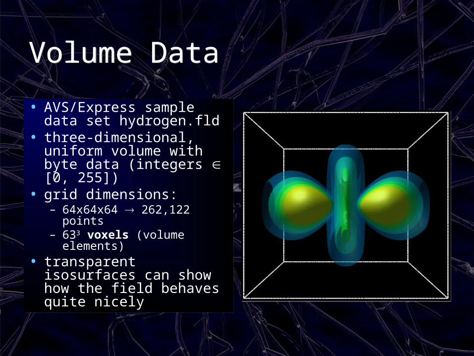
• AVS/Express sample data set hydrogen.fld
• three-dimensional, uniform volume with byte data (integers [0, 255])
• grid dimensions: – 64x64x64 262,122
points– 633 voxels (volume
elements)
• transparent isosurfaces can show how the field behaves quite nicely
• AVS/Express sample data set hydrogen.fld
• three-dimensional, uniform volume with byte data (integers [0, 255])
• grid dimensions: – 64x64x64 262,122
points– 633 voxels (volume
elements)
• transparent isosurfaces can show how the field behaves quite nicely
Volume DataVolume Data
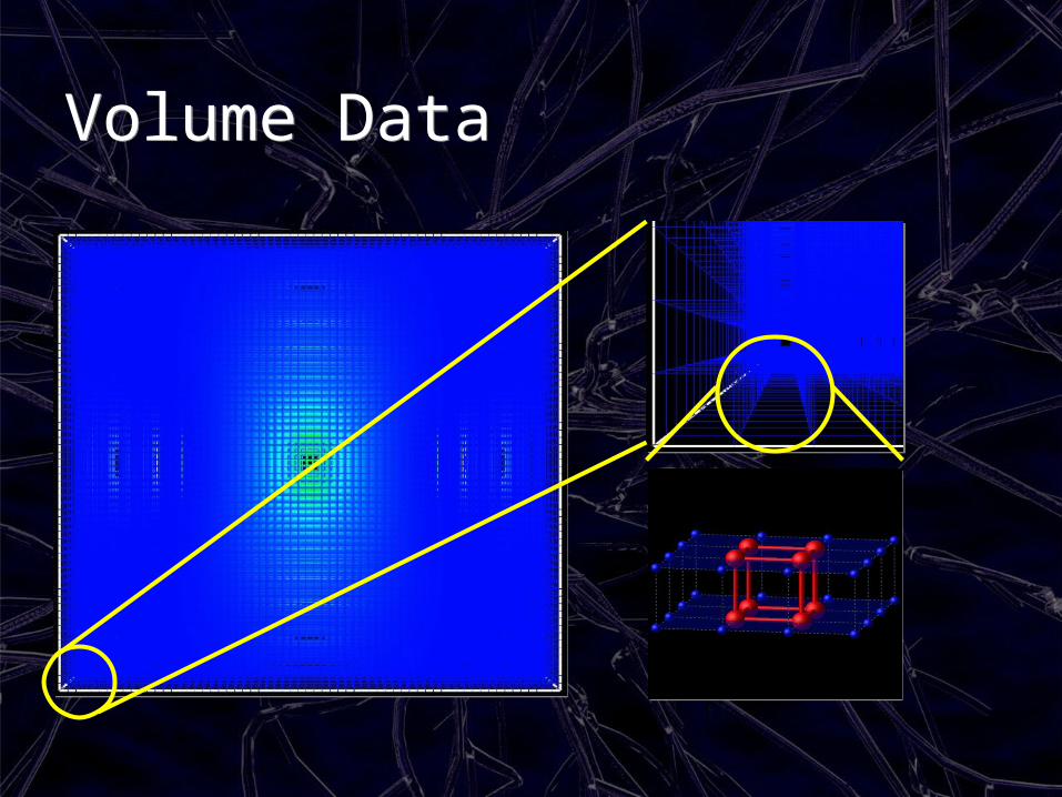
• the data values are separated by constant spacing on a Cartesian grid
• the connections are regular, forming hexahedrons (cubes in this case actually)
• the smallest connected volumes are called Voxels (volume elements)
• the data values are separated by constant spacing on a Cartesian grid
• the connections are regular, forming hexahedrons (cubes in this case actually)
• the smallest connected volumes are called Voxels (volume elements)
Volume DataVolume Data
Volume DataVolume Data
• a voxel typically has data values associated with the corner points
• to find a data value at an arbitrary location in the voxel we need to interpolate
• commonly use tri-linear interpolation
• some data sets will have a single data value for the volume (referred to as cell data)
• a voxel typically has data values associated with the corner points
• to find a data value at an arbitrary location in the voxel we need to interpolate
• commonly use tri-linear interpolation
• some data sets will have a single data value for the volume (referred to as cell data)
Volume DataVolume Data
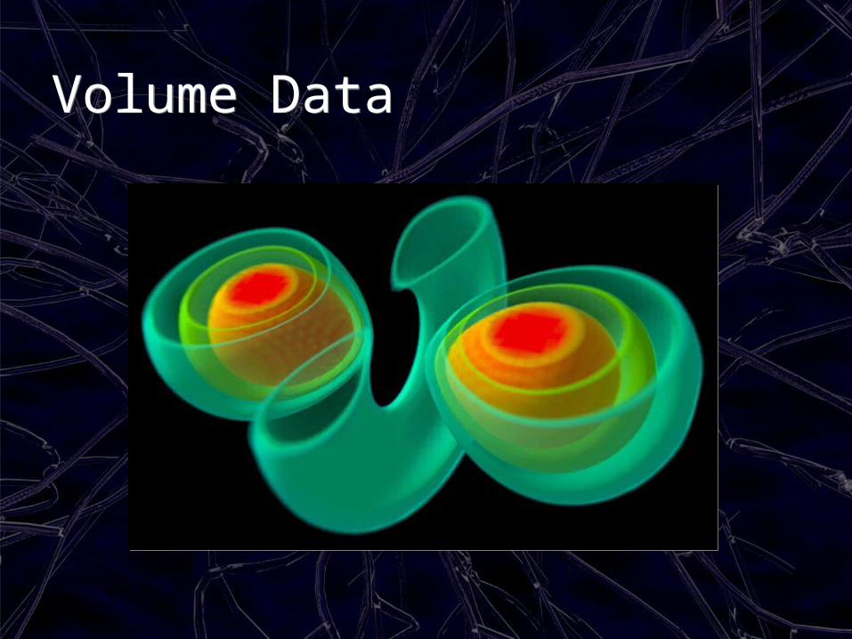
• we are now going to look at rendering volumetric data directly instead of constructing geometric primitives
• treat the volume as being composed of semitransparent material– transmits and absorbs light– light is scattered by the particles
• we are now going to look at rendering volumetric data directly instead of constructing geometric primitives
• treat the volume as being composed of semitransparent material– transmits and absorbs light– light is scattered by the particles
Volume DataVolume Data
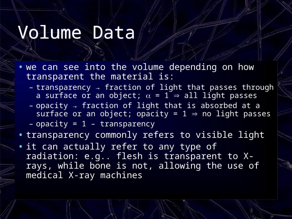
• we can see into the volume depending on how transparent the material is:– transparency → fraction of light that passes through a
surface or an object; = 1 all light passes– opacity → fraction of light that is absorbed at a
surface or an object; opacity = 1 no light passes– opacity = 1 – transparency
• transparency commonly refers to visible light• it can actually refer to any type of radiation: e.g..
flesh is transparent to X-rays, while bone is not, allowing the use of medical X-ray machines
Volume DataVolume Data
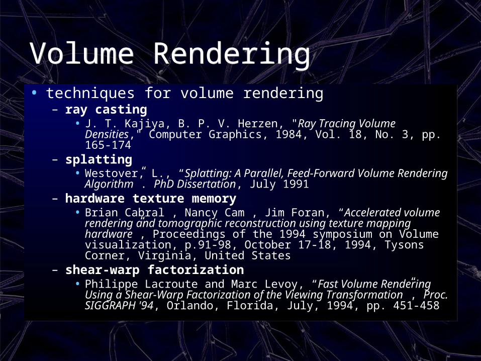
Volume RenderingVolume Rendering• techniques for volume rendering
– ray casting• J. T. Kajiya, B. P. V. Herzen, "Ray Tracing Volume Densities,"
Computer Graphics, 1984, Vol. 18, No. 3, pp. 165-174 – splatting
• Westover, L., “Splatting: A Parallel, Feed-Forward Volume Rendering Algorithm”. PhD Dissertation, July 1991
– hardware texture memory• Brian Cabral , Nancy Cam , Jim Foran, “Accelerated volume
rendering and tomographic reconstruction using texture mapping hardware”, Proceedings of the 1994 symposium on Volume visualization, p.91-98, October 17-18, 1994, Tysons Corner, Virginia, United States
– shear-warp factorization• Philippe Lacroute and Marc Levoy, “Fast Volume Rendering Using a
Shear-Warp Factorization of the Viewing Transformation”, Proc. SIGGRAPH '94, Orlando, Florida, July, 1994, pp. 451-458
• techniques for volume rendering – ray casting
• J. T. Kajiya, B. P. V. Herzen, "Ray Tracing Volume Densities," Computer Graphics, 1984, Vol. 18, No. 3, pp. 165-174
– splatting• Westover, L., “Splatting: A Parallel, Feed-Forward Volume
Rendering Algorithm”. PhD Dissertation, July 1991
– hardware texture memory• Brian Cabral , Nancy Cam , Jim Foran, “Accelerated volume
rendering and tomographic reconstruction using texture mapping hardware”, Proceedings of the 1994 symposium on Volume visualization, p.91-98, October 17-18, 1994, Tysons Corner, Virginia, United States
– shear-warp factorization• Philippe Lacroute and Marc Levoy, “Fast Volume Rendering Using a
Shear-Warp Factorization of the Viewing Transformation”, Proc. SIGGRAPH '94, Orlando, Florida, July, 1994, pp. 451-458
Ray CastingRay Casting
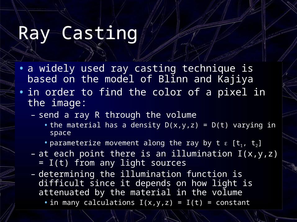
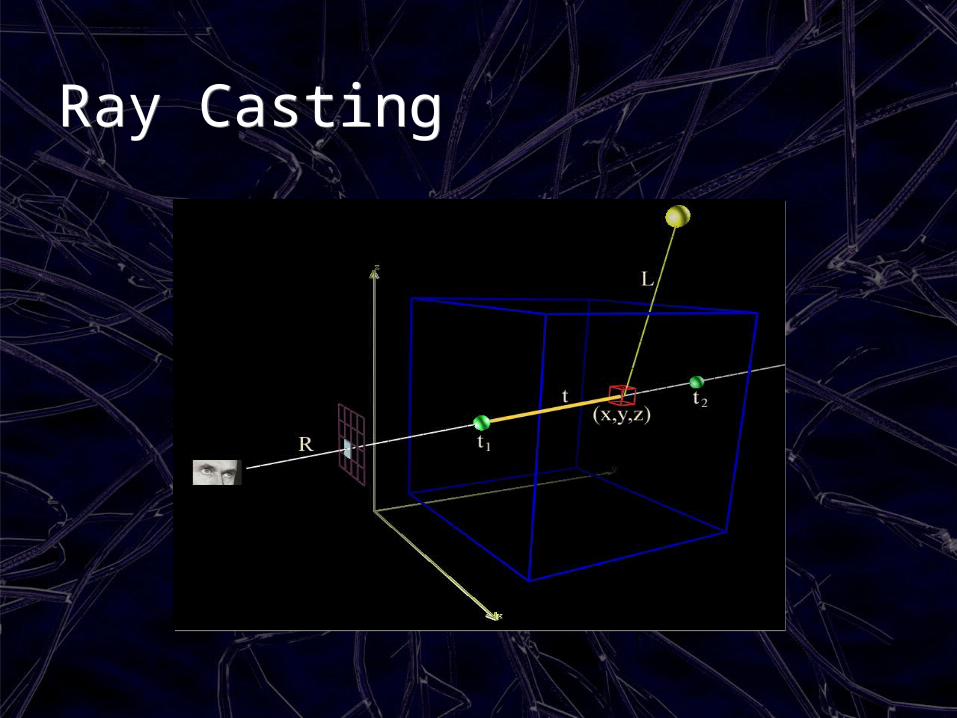
• a widely used ray casting technique is based on the model of Blinn and Kajiya
• in order to find the color of a pixel in the image:– send a ray R through the volume
• the material has a density D(x,y,z) = D(t) varying in space
• parameterize movement along the ray by t [t1, t2]
– at each point there is an illumination I(x,y,z) = I(t) from any light sources
– determining the illumination function is difficult since it depends on how light is attenuated by the material in the volume
• in many calculations I(x,y,z) = I(t) = constant
Ray CastingRay Casting
Ray CastingRay Casting
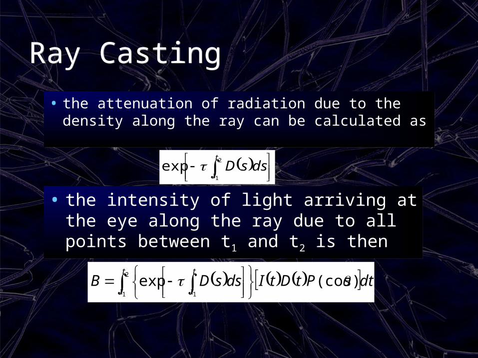
• the attenuation of radiation due to the density along the ray can be calculated as
• the attenuation of radiation due to the density along the ray can be calculated as
• the intensity of light arriving at the eye along the ray due to all points between t1 and t2 is then
• the intensity of light arriving at the eye along the ray due to all points between t1 and t2 is then
2
1
expt
tdssD
dtPtDtIdssDBt
t
t
t
2
1 1
)(cosexp
Ray CastingRay Casting
• to take away from this, in this ray casting calculation we want to find the intensity of light for a pixel in our image– calculate the attenuation of light along the ray:
integrate along the ray through the volume– calculate the intensity of light reaching the image
location – integrate along the ray again– to include lighting effects we need to calculate the
amount of light from the sources reaching each point along the ray – more integration
– multiple scattering effects – lots more integrations
Ray CastingRay Casting
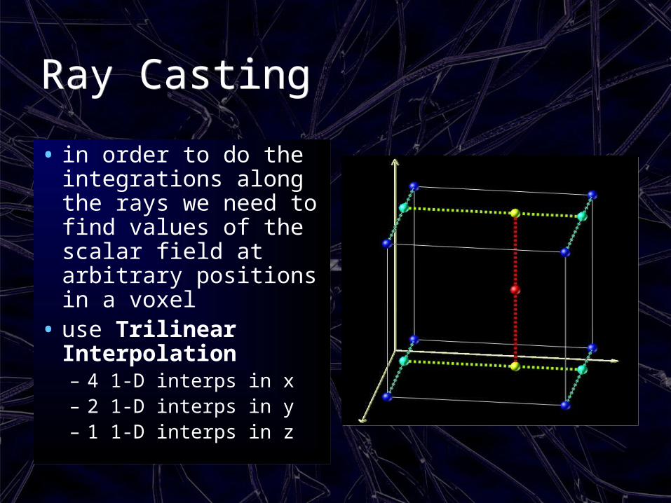
• in order to do the integrations along the rays we need to find values of the scalar field at arbitrary positions in a voxel
• use Trilinear Interpolation– 4 1-D interps in x– 2 1-D interps in y– 1 1-D interps in z
• in order to do the integrations along the rays we need to find values of the scalar field at arbitrary positions in a voxel
• use Trilinear Interpolation– 4 1-D interps in x– 2 1-D interps in y– 1 1-D interps in z
Volume Rendering – HardwareVolume Rendering – Hardware
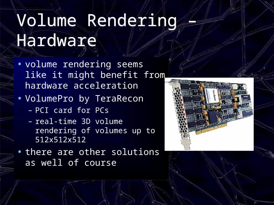
• volume rendering seems like it might benefit from hardware acceleration
• VolumePro by TeraRecon– PCI card for PCs– real-time 3D volume rendering
of volumes up to 512x512x512
• there are other solutions as well of course
• volume rendering seems like it might benefit from hardware acceleration
• VolumePro by TeraRecon– PCI card for PCs– real-time 3D volume rendering
of volumes up to 512x512x512
• there are other solutions as well of course
Volume Rendering – SoftwareVolume Rendering – Software
• many visualization packages have volume rendering capability
• AVS/Express – Advanced Visual Systems
• VTK (Visualization Toolkit) – Kitware
• VolView – based on VTK from Kitware– commercial system which focuses on volume
rendering– has support for the VolumePro card
• many visualization packages have volume rendering capability
• AVS/Express – Advanced Visual Systems
• VTK (Visualization Toolkit) – Kitware
• VolView – based on VTK from Kitware– commercial system which focuses on volume
rendering– has support for the VolumePro card
Volume RenderingVolume Rendering
• the entire body of 3D data must be processed each time an image is drawn or displayed
• imaginary "rays" are cast through the data, picking up color and opacity as they traverse it
• the rays are then projected onto a computer screen or display surface
• to make the image move or to manipulate it interactively, the data is re-processed in rapid succession, fast enough for interactive frame rates – this needs fast hardware.
Volume RenderingVolume Rendering
• in order to render a 3D volume into a 2D image we need to:– cast the rays through the volume – assign color and opacity values to the sample
points – calculate gradients and assign lighting to the
image – sum up all the color and opacity values to
create the image
• in order to render a 3D volume into a 2D image we need to:– cast the rays through the volume – assign color and opacity values to the sample
points – calculate gradients and assign lighting to the
image – sum up all the color and opacity values to
create the image
Computed Tomography (CT)Computed Tomography (CT)
• Computed Tomography (CT) or Computed Axial Tomography (CAT)
• uses a combination of X-rays and computer technology to produce cross-sectional images of the body
• an x-ray tube rotates in a circle around the patient, making many pictures as it rotates
• final slice images are generated utilizing the basic principle that the internal structure of the body can be reconstructed from multiple X-ray projections
• physicians can then examine “slices” through different organs and show detailed images of any part of the body
Computed Tomography (CT)Computed Tomography (CT)
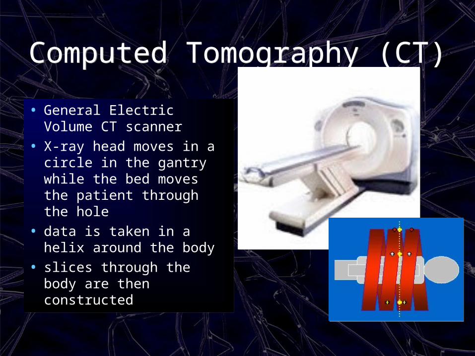
• General Electric Volume CT scanner
• X-ray head moves in a circle in the gantry while the bed moves the patient through the hole
• data is taken in a helix around the body
• slices through the body are then constructed
• General Electric Volume CT scanner
• X-ray head moves in a circle in the gantry while the bed moves the patient through the hole
• data is taken in a helix around the body
• slices through the body are then constructed
Computed Tomography (CT)Computed Tomography (CT)
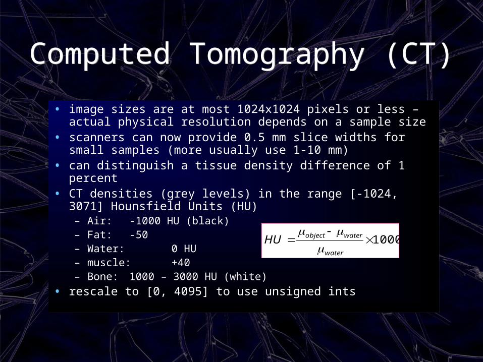
• image sizes are at most 1024x1024 pixels or less – actual physical resolution depends on a sample size
• scanners can now provide 0.5 mm slice widths for small samples (more usually use 1-10 mm)
• can distinguish a tissue density difference of 1 percent• CT densities (grey levels) in the range [-1024, 3071]
Hounsfield Units (HU)– Air: -1000 HU (black)– Fat: -50– Water: 0 HU– muscle: +40– Bone: 1000 – 3000 HU (white)
• rescale to [0, 4095] to use unsigned ints
1000
water
waterobjectHU
Computed Tomography (CT)Computed Tomography (CT)
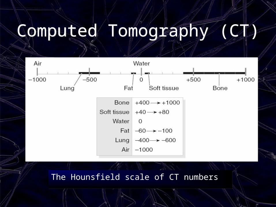
The Hounsfield scale of CT numbersThe Hounsfield scale of CT numbers
Computed Tomography (CT)Computed Tomography (CT)
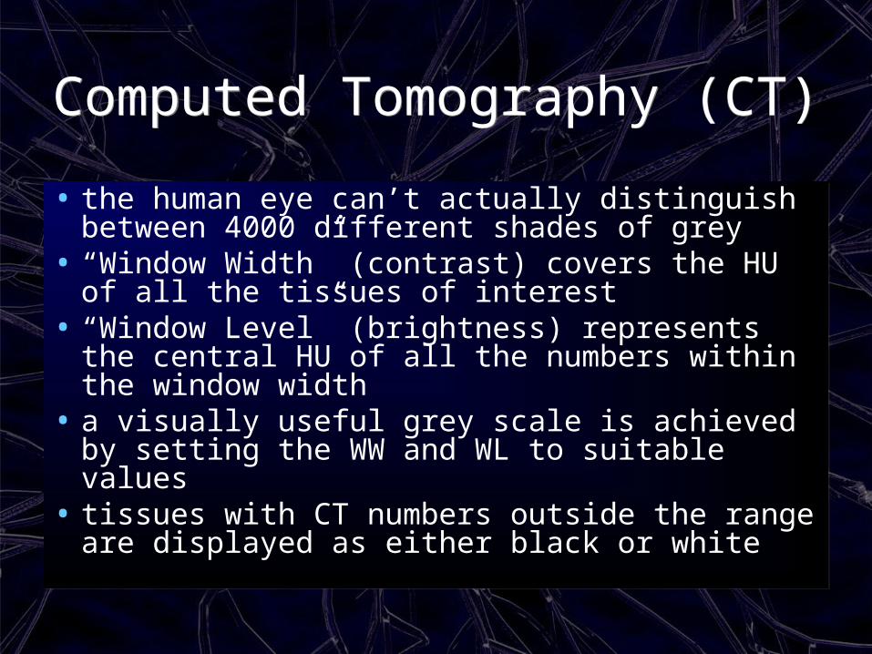
• the human eye can’t actually distinguish between 4000 different shades of grey
• “Window Width” (contrast) covers the HU of all the tissues of interest
• “Window Level” (brightness) represents the central HU of all the numbers within the window width
• a visually useful grey scale is achieved by setting the WW and WL to suitable values
• tissues with CT numbers outside the range are displayed as either black or white
Computed Tomography (CT)Computed Tomography (CT)
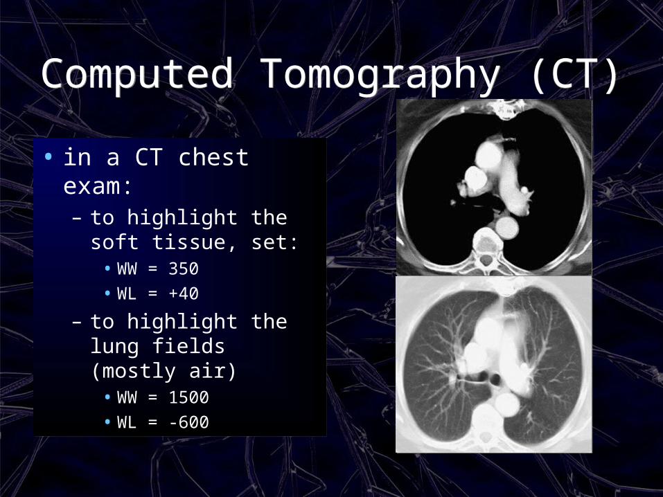
• in a CT chest exam:– to highlight the soft
tissue, set:• WW = 350
• WL = +40
– to highlight the lung fields (mostly air)
• WW = 1500
• WL = -600
• in a CT chest exam:– to highlight the soft
tissue, set:• WW = 350
• WL = +40
– to highlight the lung fields (mostly air)
• WW = 1500
• WL = -600
Other Volume Data SourcesOther Volume Data Sources
• lots of bio-medical measurement sources– Magnetic Resonance Imaging (MRI) – Positron Emission Tomography (PET) – Single Photon Emission Computed
Tomography (SPECT, ECT) – Ultrasound Imaging – 2-D and 3-D Microscopy Imaging (Light,
Electron, Confocal, Atomic Force)
• lots of bio-medical measurement sources– Magnetic Resonance Imaging (MRI) – Positron Emission Tomography (PET) – Single Photon Emission Computed
Tomography (SPECT, ECT) – Ultrasound Imaging – 2-D and 3-D Microscopy Imaging (Light,
Electron, Confocal, Atomic Force)
Other Volume Data SourcesOther Volume Data Sources
• measurements– seismic data– atmospheric data
• scientific modeling– plasma physics– atmospheric modeling– geophysical earth models
• plenty of others
• measurements– seismic data– atmospheric data
• scientific modeling– plasma physics– atmospheric modeling– geophysical earth models
• plenty of others
Medical Data - DICOMMedical Data - DICOM
• Digital Imaging and Communications in Medicine (DICOM)
• main objective of this standard is to create a vendor independent platform for the communication of medical images and related data
• http://medical.nema.org/dicom/
• Digital Imaging and Communications in Medicine (DICOM)
• main objective of this standard is to create a vendor independent platform for the communication of medical images and related data
• http://medical.nema.org/dicom/
Medical Data - DICOMMedical Data - DICOM
• a set of rules that allow medical images to be exchanged between instruments, computers, and hospitals
• a DICOM file contains:– a header
• stores information about the patient's name, the type of scan, image dimensions, etc.
– all of the image data • which can contain information in three dimensions
Example – CT scanExample – CT scan
• VolView from Kitware– based on the Visualization Toolkit
• look at sample data from the University of North Carolina• Description: CT study of a cadaver head
– Dimensions: 113 slices of 256 x 256 pixels,voxel grid is rectangular, andX:Y:Z aspect ratio of each voxel is 1:1:2
– Files: 113 binary files, one file per slice– File format: 16-bit integers (Mac byte ordering), file contains no
header– Data source: acquired on a General Electric CT Scanner and
provided courtesy of North Carolina Memorial Hospital
Example – CT scanExample – CT scan
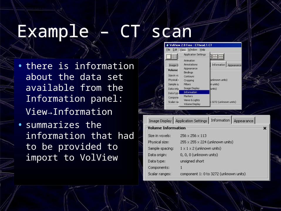
• there is information about the data set available from the Information panel:
View→Information
• summarizes the information that had to be provided to import to VolView
• there is information about the data set available from the Information panel:
View→Information
• summarizes the information that had to be provided to import to VolView
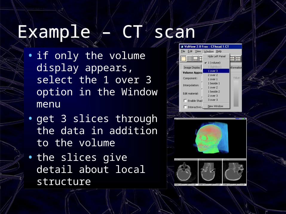
Example – CT scanExample – CT scan• if only the volume display
appears, select the 1 over 3 option in the Window menu
• get 3 slices through the data in addition to the volume
• the slices give detail about local structure
• if only the volume display appears, select the 1 over 3 option in the Window menu
• get 3 slices through the data in addition to the volume
• the slices give detail about local structure
Example – CT scanExample – CT scan
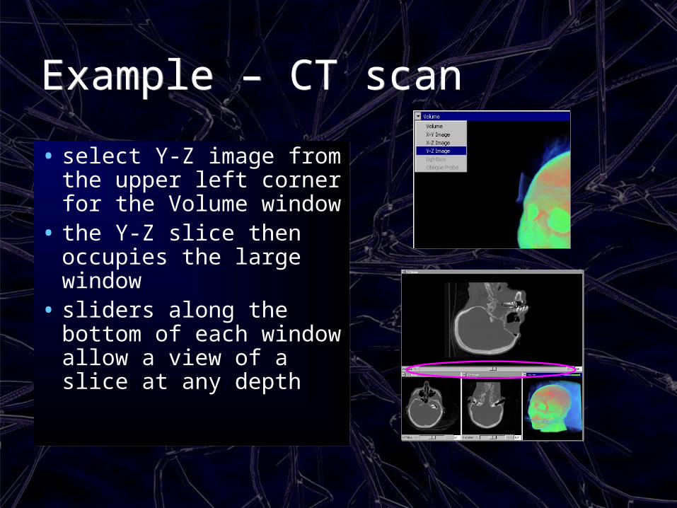
• select Y-Z image from the upper left corner for the Volume window
• the Y-Z slice then occupies the large window
• sliders along the bottom of each window allow a view of a slice at any depth
• select Y-Z image from the upper left corner for the Volume window
• the Y-Z slice then occupies the large window
• sliders along the bottom of each window allow a view of a slice at any depth
Example – CT scanExample – CT scan
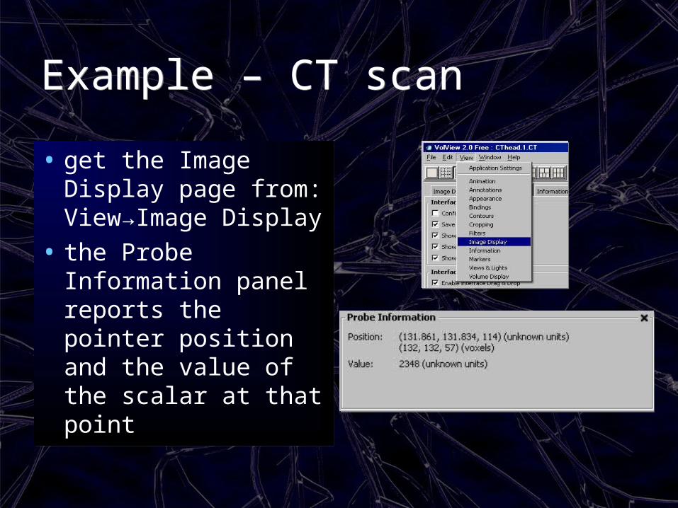
• get the Image Display page from: View→Image Display
• the Probe Information panel reports the pointer position and the value of the scalar at that point
• get the Image Display page from: View→Image Display
• the Probe Information panel reports the pointer position and the value of the scalar at that point
Example – CT scanExample – CT scan
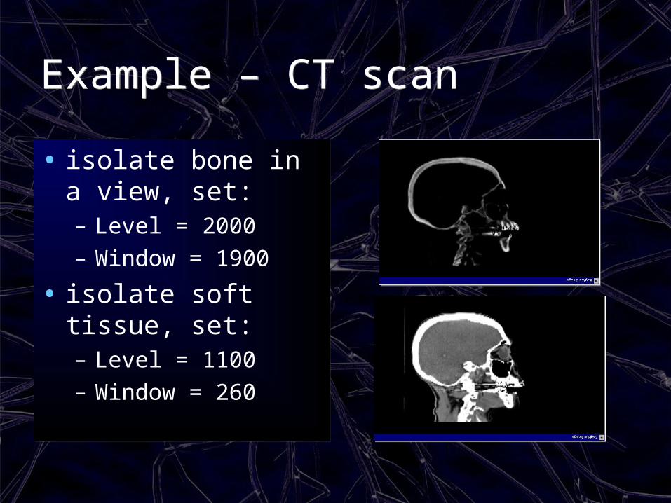
• isolate bone in a view, set:– Level = 2000– Window = 1900
• isolate soft tissue, set:– Level = 1100– Window = 260
• isolate bone in a view, set:– Level = 2000– Window = 1900
• isolate soft tissue, set:– Level = 1100– Window = 260
Example – CT scanExample – CT scan
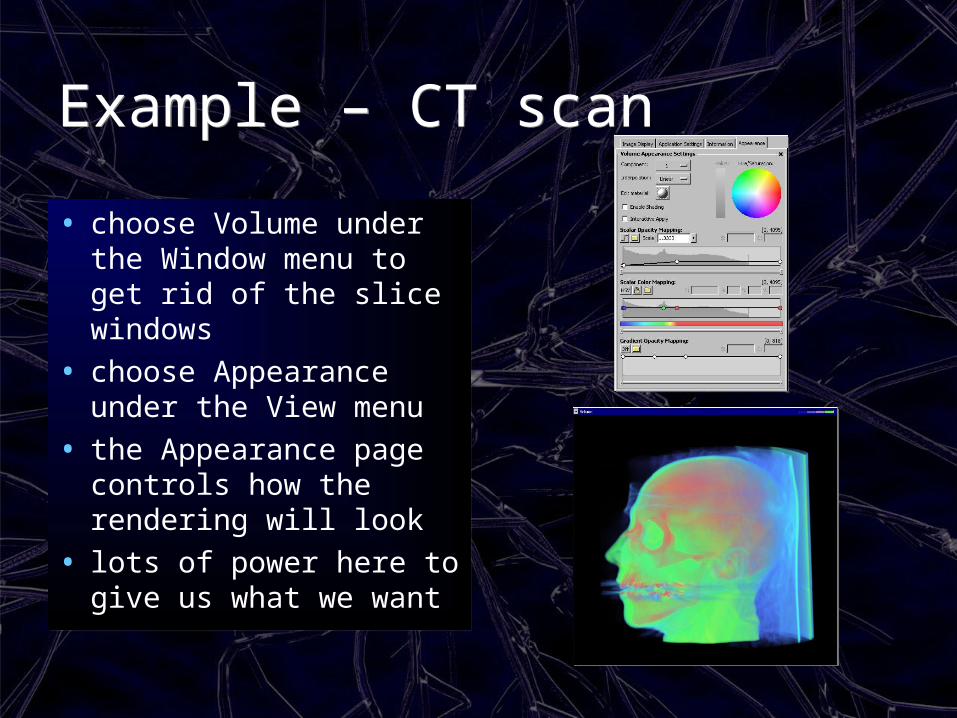
• choose Volume under the Window menu to get rid of the slice windows
• choose Appearance under the View menu
• the Appearance page controls how the rendering will look
• lots of power here to give us what we want
• choose Volume under the Window menu to get rid of the slice windows
• choose Appearance under the View menu
• the Appearance page controls how the rendering will look
• lots of power here to give us what we want
Example – CT scanExample – CT scan
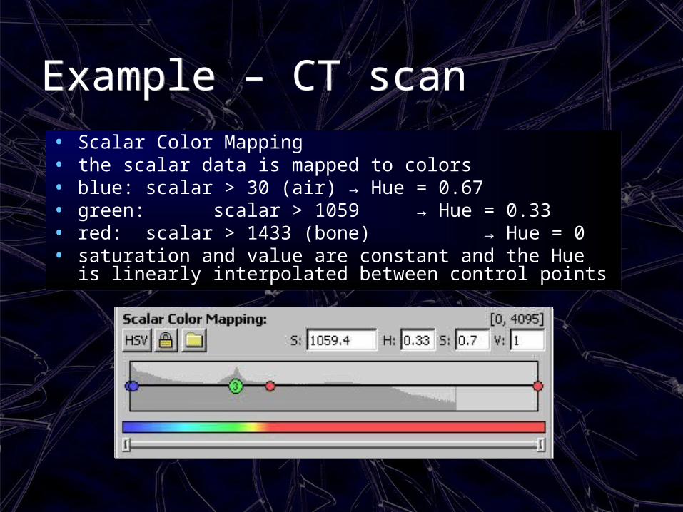
• Scalar Color Mapping• the scalar data is mapped to colors• blue: scalar > 30 (air) → Hue = 0.67 • green: scalar > 1059 → Hue = 0.33• red: scalar > 1433 (bone) → Hue = 0• saturation and value are constant and the Hue is linearly
interpolated between control points
• Scalar Color Mapping• the scalar data is mapped to colors• blue: scalar > 30 (air) → Hue = 0.67 • green: scalar > 1059 → Hue = 0.33• red: scalar > 1433 (bone) → Hue = 0• saturation and value are constant and the Hue is linearly
interpolated between control points
Example – CT scanExample – CT scan
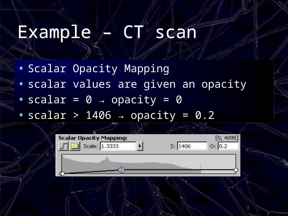
• Scalar Opacity Mapping
• scalar values are given an opacity
• scalar = 0 → opacity = 0
• scalar > 1406 → opacity = 0.2
• Scalar Opacity Mapping
• scalar values are given an opacity
• scalar = 0 → opacity = 0
• scalar > 1406 → opacity = 0.2
Example – CT scanExample – CT scan
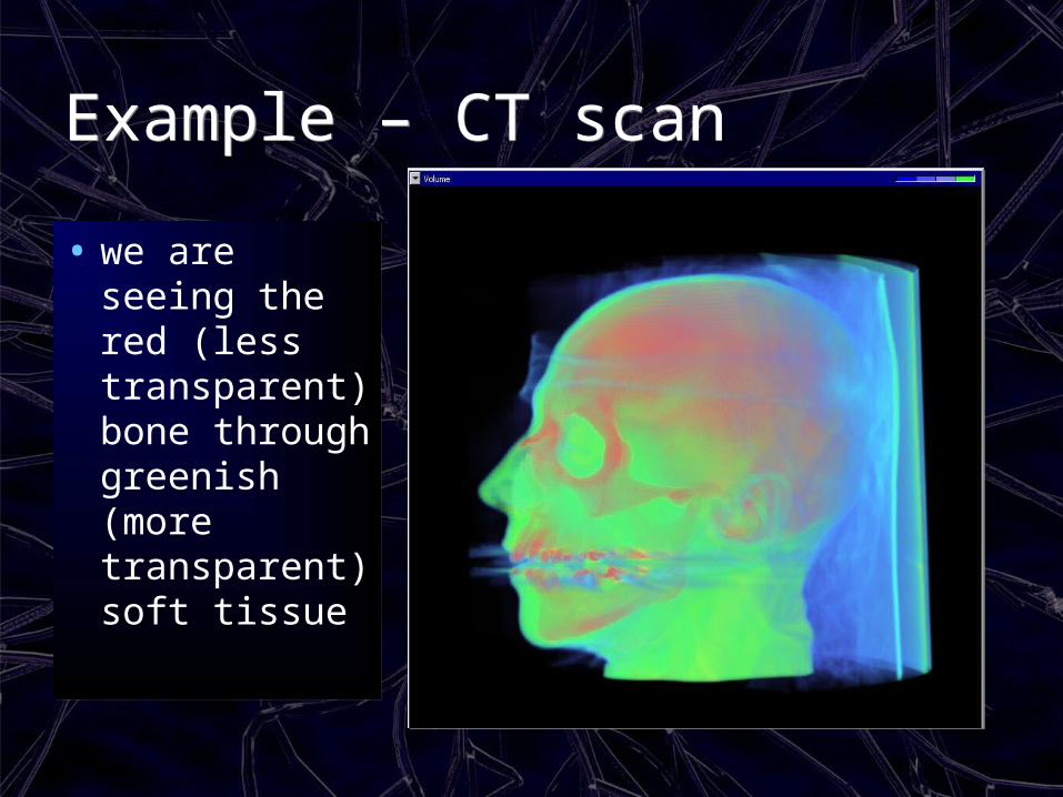
• we are seeing the red (less transparent) bone through greenish (more transparent) soft tissue
• we are seeing the red (less transparent) bone through greenish (more transparent) soft tissue
Example – CT scanExample – CT scan
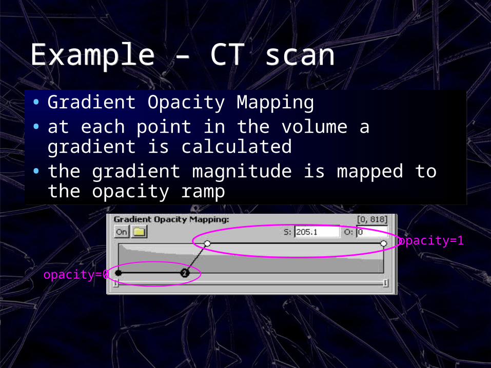
• Gradient Opacity Mapping• at each point in the volume a gradient is
calculated• the gradient magnitude is mapped to the opacity
ramp
• Gradient Opacity Mapping• at each point in the volume a gradient is
calculated• the gradient magnitude is mapped to the opacity
ramp
opacity=0
opacity=1
Example – CT scanExample – CT scan
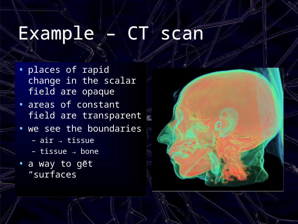
• places of rapid change in the scalar field are opaque
• areas of constant field are transparent
• we see the boundaries– air → tissue– tissue → bone
• a way to get “surfaces”
• places of rapid change in the scalar field are opaque
• areas of constant field are transparent
• we see the boundaries– air → tissue– tissue → bone
• a way to get “surfaces”
Example – CT scanExample – CT scan
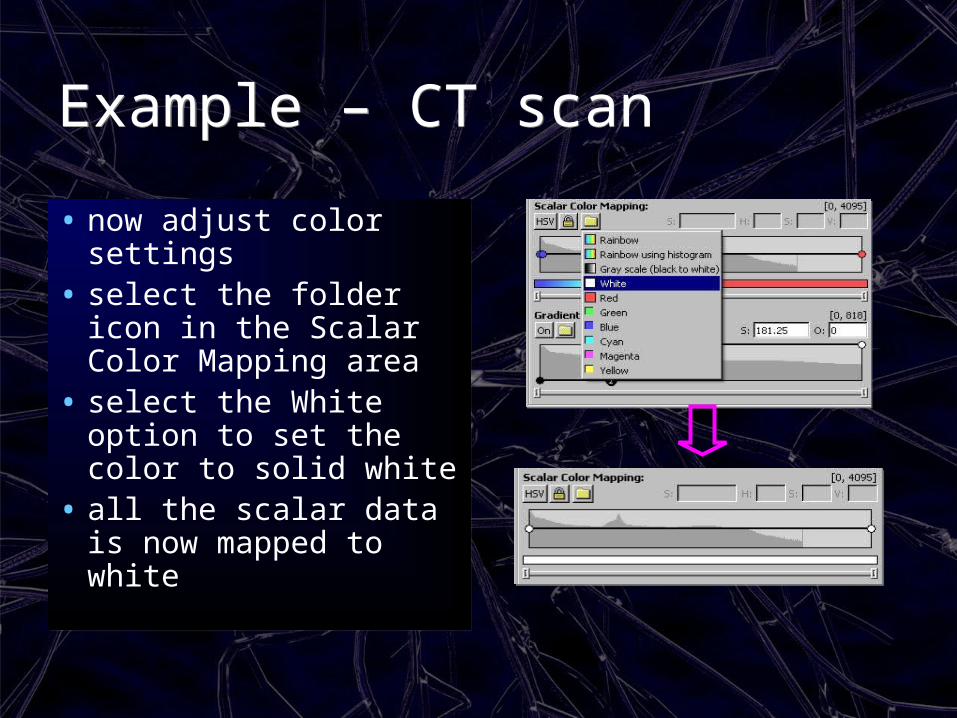
• now adjust color settings
• select the folder icon in the Scalar Color Mapping area
• select the White option to set the color to solid white
• all the scalar data is now mapped to white
• now adjust color settings
• select the folder icon in the Scalar Color Mapping area
• select the White option to set the color to solid white
• all the scalar data is now mapped to white
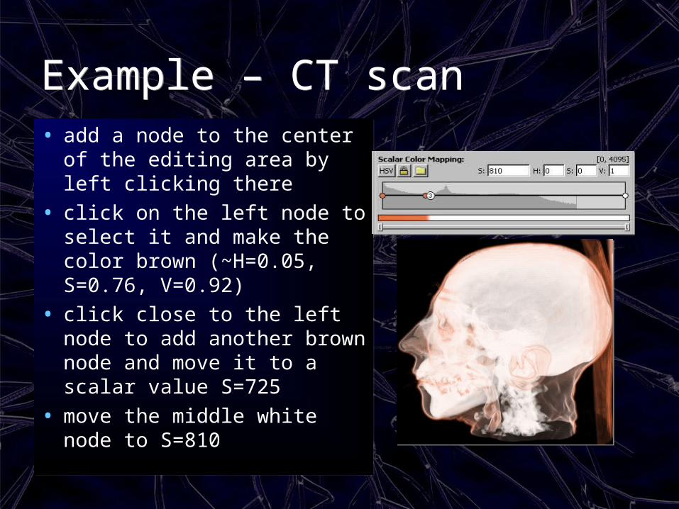
Example – CT scanExample – CT scan• add a node to the center of
the editing area by left clicking there
• click on the left node to select it and make the color brown (~H=0.05, S=0.76, V=0.92)
• click close to the left node to add another brown node and move it to a scalar value S=725
• move the middle white node to S=810
• add a node to the center of the editing area by left clicking there
• click on the left node to select it and make the color brown (~H=0.05, S=0.76, V=0.92)
• click close to the left node to add another brown node and move it to a scalar value S=725
• move the middle white node to S=810
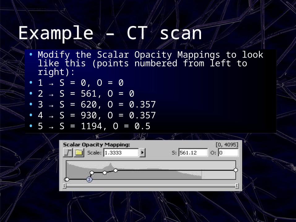
Example – CT scanExample – CT scan• Modify the Scalar Opacity Mappings to look like this
(points numbered from left to right):• 1 → S = 0, O = 0• 2 → S = 561, O = 0• 3 → S = 620, O = 0.357• 4 → S = 930, O = 0.357• 5 → S = 1194, O = 0.5
• Modify the Scalar Opacity Mappings to look like this (points numbered from left to right):
• 1 → S = 0, O = 0• 2 → S = 561, O = 0• 3 → S = 620, O = 0.357• 4 → S = 930, O = 0.357• 5 → S = 1194, O = 0.5
Example – CT scanExample – CT scan
Example – CT scanExample – CT scan
• the Appearance panel in VolView 2.0 is the most complex interface
• it defines the core parameters that affect the volume rendered image
• this is where the control is for effectively visualizing data!
• the Appearance panel in VolView 2.0 is the most complex interface
• it defines the core parameters that affect the volume rendered image
• this is where the control is for effectively visualizing data!
ConclusionConclusion
• Volume rendering is a powerful tool for visualization and can assist in understanding volumetric data sets
• useful to add to the toolkit to compliment the geometric techniques that we’ve seen earlier.
• Volume rendering is a powerful tool for visualization and can assist in understanding volumetric data sets
• useful to add to the toolkit to compliment the geometric techniques that we’ve seen earlier.


