AN AGENT-BASED HYBRID MODEL FOR AVASCULAR TUMOR GROWTH

AARON C. ABAJIANADVISOR: PROFESSOR JOHN S. LOWENGRUB

Abstract. Tumor development is a complex and multi-faceted process that cannot be captured in a singleformula, yet the ability to predict a maturing tumor’s magnitude and direction of growth would providesignificant clinical benefits. In-vitro trials provide only limited predictive data since it is nearly impossibleto chemically reproduce the exact environmental conditions surrounding a tumor. Moreover, each trial isnecessarily unique to a specific tumor and cannot be quickly modified to satisfy the requirements of another.Mathematical models provide a virtual solution to this problem by implementing the core processes oftumor development in software. We present a model for tumor development from the single-cell stage toearly microinvasion. An overlying nutrient field determines a cell’s status as living, quiescent, or nonviable.Interactions between tumor cells are simulated using a competing exponential function and nutrient influxis modeled using the diffusion equation. The model may be applied to a variety of emerging tumors bycarefully defining the set of constants that determines the tumor’s development pathway.

1. Introduction

1.1. Cancer. Cancer afflicted a reported 1.44 million individuals within the United States during 2007[3]. These cases encompassed the majority of organ systems in the human body. In each case, tumordevelopment occurs along a characteristic pathway, yet affective treatment options are often limited to thetype and localization of the tumor. Generalized chemotherapeutic agents combat a broader selection ofcancers by targeting the characteristic behaviors commonly seen in abnormal tissue.

The largest class of chemotherapeutic medications counters tumor cells that are overactive consumers.The mutations leading to the development of a tumor cell are often located in growth or proliferationgenes and consequently induce the cell to rapidly consume nutrients within its vicinity. A toxic agentintroduced into the patient’s body is globally absorbed, but at a faster rate by cells mutant for theconsumption gene. The rate of consumption of a particular substance depends upon cellular phenotypesand the extracellular environment. These parameters must be considered when defining an appropriatedosage for a chemotherapeutic agent. The optimal solution would be a dosage sufficient to eradicate thezealous tissue while exhibiting little to no harmful effects on the nearby normal tissue.

This seemingly complex problem may be reduced to the two-variable system involving the competitionbetween the rate of drug diffusion in solution and the rate of cellular uptake. The former may be measuredin vitro while the latter depends upon a cell’s phenotype. The rate of uptake by normal cells is expectedto be lesser than that of mutant cells. The modeling challenge is to describe the rate of consumption ofchemotherapeutic as a function of the tumor mass at any given time. A comparison may then be madeagainst the basal uptake rate by normal tissue to determine the sufficient dosage for a tumor at its currentstage. The uptake rate of a tumor at a given stage is clearly the result of its development pathway.

1.2. Tumor Development. The development of an invasive tumor from normal tissue is a elaborateprocess that roughly divides into three stages. Stage 1 - A healthy cell must first accumulate a collectionof mutations in a specific family of genes (1.2.1). The mutant cell then becomes the ancestral parentof a strain of mutated cells that forms a spherical mass isolated from the surrounding tissue. Stage 2 -Peripheral tumor cells deplete the nutrient supply as it diffuses into the spherical tumor. Central tumorcells are nutrient deprived resulting in a characteristic necrotic core (1.2.2). The tumor continues tothrive through the rapid division of viable cells on the sphere periphery. Stage 3 - Environmental factorssignal the peripheral cells to invade the surrounding tissue and/or to release chemical agents that induce

1

2 AARON C. ABAJIAN ADVISOR: PROFESSOR JOHN S. LOWENGRUB

the formation of nearby blood vessels. Metastasis of the tumor occurs locally (microinvasion) throughindividual cell movement or system-wide (macroinvasion) through the bloodstream (1.2.3).

1.2.1. Accumulation of Mutations. Tumor development begins when a single cell accumulates mutationsin a set of critical genes. Several mutations are usually necessary to affect the change from normal toabnormal growth. The essential sets of genes implicated in tumor developed are the tumor suppressorand oncogene families. These genes code for proteins that control cell proliferation and growth. A loss-of-function mutation in a tumor suppressor gene or a gain-of-function mutation in an oncogene may increasethe division rate or the lifespan of the affected cell. A cell that proliferates incessantly or that ignoressignals from other cells (esp. apoptotic signals) may give rise to a lineage of invasive cells.

1.2.2. Necrotic Core Formation. The rapid division of the initial mutant cell results in the logistic growthof a spherical tumor. Studies have indicated that, although tumor cells do not respond to signals fromnormal cells, they do exhibit adhesion to one another. The close proximity of highly competitive cellsresults in the depletion of the local nutrient concentration. Cells stranded in the center of a tumor massare starved for nutrients and form a necrotic central region. The tumor displays the characteristic three-layer structure of viable, quiescent, and necrotic cells as a dynamic equilibrium is reached between diffusivenutrient influx and cellular nutrient consumption.

1.2.3. Invasion. The starvation of inner tumor cells leads to their competitive advance. These cells mayencroach upon the surrounding tissue or release signaling molecules that promote the growth of nearbyblood vessels. Microinvasive encroachment is a localized phenomena that is performed by phenotypicallymutant cells. The mutation allows the cells to successfully detach from the spherical tumor mass. Amacroinvasive cell may release Vascular Endothelial Growth Factors (VEGFs) that induce endothelial cellsto form vessels towards the tumor. VEGFs are signaling proteins that normally play benign roles but alsofunction as an abnormal cell’s response to nutrient deprivation. The process by which tumor cells gainaccess to the blood supply is termed vascularization.

1.3. Mathematical Models. The three stages of tumor development are the result of complex intra-cellular, intercellular, and extracellular processes. The inherent difficulty of reducing each stage intoscientifically useful pieces has given rise to sophisticated tumor models. The goal of an abstract model isto understand a complex system that cannot be appreciated using the typical ‘pen-and-paper’ approach.In biology, the existence of multiple inhibitors and repressors for a single gene provides an immediateappreciation for the utility of a calibrated model. An initial concentration and spatial distribution maybe specified for each enzyme and the resulting gene activity calculated without in-vitro experimentation.Similarly, a thoroughly development tumor model could provide preemptive information about a tumor’sdevelopment pathway. Models aiming to achieve this goal are still in their infancy and are broadly classi-fied as either continuous (1.3.1) or discrete (1.3.2). Models that incorporate features from both classes aretermed hybrid models (1.3.3).

1.3.1. Continuous Models. A continuous model is defined by partial differential equations (PDEs) thatgovern the evolution of a tumor mass. The tumor’s physical dimensions and growth rate are measured andvisually displayed without reference to the behavior of the underlying cells. Continuous models sacrificethe maintenance of cell specific properties in favor of computational speed.

1.3.2. Discrete Models. Portions of a discrete model may be based off of continuous PDEs, but the heartof a discrete model is the maintenance of disjoint units of information that change over time and sum toproduce the overall system. Time itself is broken into constant steps rather than allowing for a continuousprogression. An agent-based discrete model focuses upon the individual objects affecting a system’s evo-lution. An agent-based population model would store location and genotypic/phenotypic information forevery member of the species within the region of interest. Population trends would be calculated basedupon the pairwise interactions between individuals over time, rather than an overall PDE describing thepopulation mass. This modeling approach is computationally demanding but provides greater insight intothe constructed nature of the system.

AN AGENT-BASED HYBRID MODEL FOR AVASCULAR TUMOR GROWTH 3

1.3.3. Hybrid Models. A combination of continuous and discrete modeling techniques provides the benefitsof both implementations within the same simulation. A discrete model for the distribution of bacteriaafter exposure to an antibiotic could model individual cells by biasing their proliferation and viabilityaccording to the drug’s spatial distribution. This agent-based model could be extended by incorporating thecontinuous diffusion equation to describe the movement of the antibiotic down its concentration gradient.The resulting hybrid model would simulate the bacteria’s response to a diffusing antibiotic in solution.

2. Mathematical Model

We present avascular tumor development as a two-dimensional hybrid continuum/discrete agent-basedmodel. Our model simulates the development pathway from a single cell (1.2.1) to the formation of astable necrotic region (1.2.2) and proceeds to the early stages of microinvasion (1.2.3). Cells function asthe component agents whose properties are maintained. Stored cell data includes spatial, genotypic, andphenotypic information. The diffusion PDE is used to model the competition between diffusive nutrientinflux and cellular nutrient uptake. Tumor cells adhere and repel from one another via the potentialinteraction equation previously described by Chuang et. al. [1]. Temporal progression occurs throughdiscretized time-steps. Figure 1 provides an overview of the processes that occur within a single time-step.

A common set of calculations is performed on the cells during each time-step (2.1). These calculationsinclude routine tasks such as verifying viability and quiescence statuses (yellow blocks, 2.1.1) and checkingfor mitosis (blue blocks, 2.1.2). The lower orange blocks in Figure 1 refer to processes that affect cellularmovement (2.2). These processes include intercellular forces (2.2.1), haptotaxis, and chemotaxis (2.2.2).Cell positions are updated after the last iteration through the loop. The nutrient concentration describedby the PDE is allowed to reach equilibrium prior to the next time-step (red block, 2.3). The diffusive influxof nutrients is discussed in Section 2.3.1 while cellular uptake of nutrient is described in Section 2.3.2.

2.1. Cell Calculations. The model maintains a set of physical variables for each cell. Table 1 provides alist of these properties along with their default values as specified for the initial cell. The values of theseproperties collectively determine the cell’s division, localized movement, and invasion rates during eachtime-step.

Table 1. List of viability parameters maintained for every cell along with their non-dimensionalized default values.

Cell Class Variables

Variable Initial ValueSpeed 1.000Age 0.000Time until next cell division 0.083Mitosis period 0.083Lifespan ∞Generation Number 0.000Maximum Generation ∞Current position in space (0, 0, 0)Local nutrient concentration 1.000Quiescent NoContains genomic mutation NoLiving Yes

2.1.1. Physical Variables. A cell remains alive and capable of dividing as long as there is sufficient nutrientin its vicinity. If the local nutrient concentration drops below the quiescence threshold, Tq, the cell losesits ability to divide. Quiescent cells have a slower metabolic rate that is modeled by a decreased rate ofnutrient consumption. Microinvasive tumor cells arise from quiescent cells undergoing extreme nutrientdeprivation. If the nutrient concentration falls below the viability threshold, Td, the cell dies.

4 AARON C. ABAJIAN ADVISOR: PROFESSOR JOHN S. LOWENGRUB

Begin Time StepCell Calculations

(2.1)Nutrient Solver

(2.3.1) and (2.3.2)

Next Cell, i

Cell alive?

Ni > Tm?Cell Dies

Ni > Tq?Cell Quiescence

Mutate?Phenotypic

Change

Mitosis Checks(2.1.2)

Aged?

Space?

Divide

Intercellular Forces(2.2.1)

Mutant?Degrade

Fibronectin

Haptotaxis andChemotaxis

(2.2.2)

Last Cell?

Update CellPositions

Yes

No

No

No

Yes

Yes

No

Yes

Yes

No

Yes

No

No Yes

No

Yes

Figure 1. Overall simulation flowchart. The symbol Ni denotes the nutrient concentrationaround cell i. Tm refers to the viability threshold while Tq refers to the quiescence threshold.

AN AGENT-BASED HYBRID MODEL FOR AVASCULAR TUMOR GROWTH 5

The starvation of tumor cells has been implicated in the microinvasion pathway (ref?). We model thisphenomena by inducing a phenotypic mutation in randomly chosen quiescent cells. A phenotypicallymodified cell detaches from the tumor mass and migrates up the nutrient gradient by degrading the localfibronectin concentration. See Section 2.2.2 for further information.

2.1.2. Mitosis. A cell undergoes mitosis if several conditions are met. First, the cell must not be quiescentor a phenotypic mutant as determined by the previous checks. There is also a minimum waiting period afterthe cell’s previous division. This check ensures that the cell has had enough time to perform the essentialstages of the cell cycle. The waiting period for division is dependent on the local nutrient concentration.This models the increased time it takes a cell to acquire sufficient resources to divide in a nutrient-deficientenvironment.

The last mitosis check verifies that there is sufficient space around the parent cell. Physically, a cellcannot divide when it is spatially constrained by adjacent cells. This phenomenon is taken into accountby examining the cell’s repulsion coefficient from the potential interactions equation (2.2.1). The repulsioncoefficient must be below a constant threshold to permit division. A cell that passes all of the checkpointsdivides into two daughter cells. A new cell is added to the cell array with identical parameters to that ofthe parent except for location. The new cell’s position is a small random offset of the parent’s position.

2.2. Cell Movement. Selected cells move a random amount according to the Gaussian Normal Distri-bution with mean zero and standard deviation equal to the square of the time-step size. These cells alsomove in response to the forces exerted on them by nearby cells and in response to chemical and nutrientgradients. These biasing agents influence the velocity of a cell. In general, we may express the continuousposition of a cell at time t as:

(1) ~x (t) =

∫ t

0

~v (s) ds

Where ~v (t) is the velocity vector of the cell at time t. In order to discretize this formula, suppose that wewish to update a cell’s position for the nth time-step given that we are on time-step n− 1. We may splitthe integral along this time:

(2) ~x (n∆t) =

Cell position at time-step (n− 1).︷ ︸︸ ︷∫ (n−1)∆t

0

~v (s) ds +

Displacement of cell during nth time-step.︷ ︸︸ ︷∫ n∆t

(n−1)∆t

~v (s) ds

Note that ∆t in this case denotes the size of one time-step. The first integral represents the cell’s positionat time-step n− 1:

(3) ~x (n∆t) = ~x((n− 1) ∆t) +

∫ n∆t

(n−1)∆t

~v (s) ds

For ∆t sufficiently small, we may approximate the right integral by the product ~v (n∆t) ∆t:

(4) ~x (n∆t) = ~x((n− 1) ∆t) + ~v (n∆t) ∆t

This is the discretized formula for calculating a cell’s position at time n∆t given the cell’s position at theprevious time-step. The value of the velocity vector at time n∆t is determined by the sum of velocityvectors from each biasing agent:

(5) ~v = DI~vI +DH~vH +DC~vC

The subscripts I, H, and C stand for intercellular interactions, haptotaxis, and chemotaxis, respectively.DX is a constant coefficient defined for biasing agent X. The velocity components are described in detailin the following sections.

6 AARON C. ABAJIAN ADVISOR: PROFESSOR JOHN S. LOWENGRUB

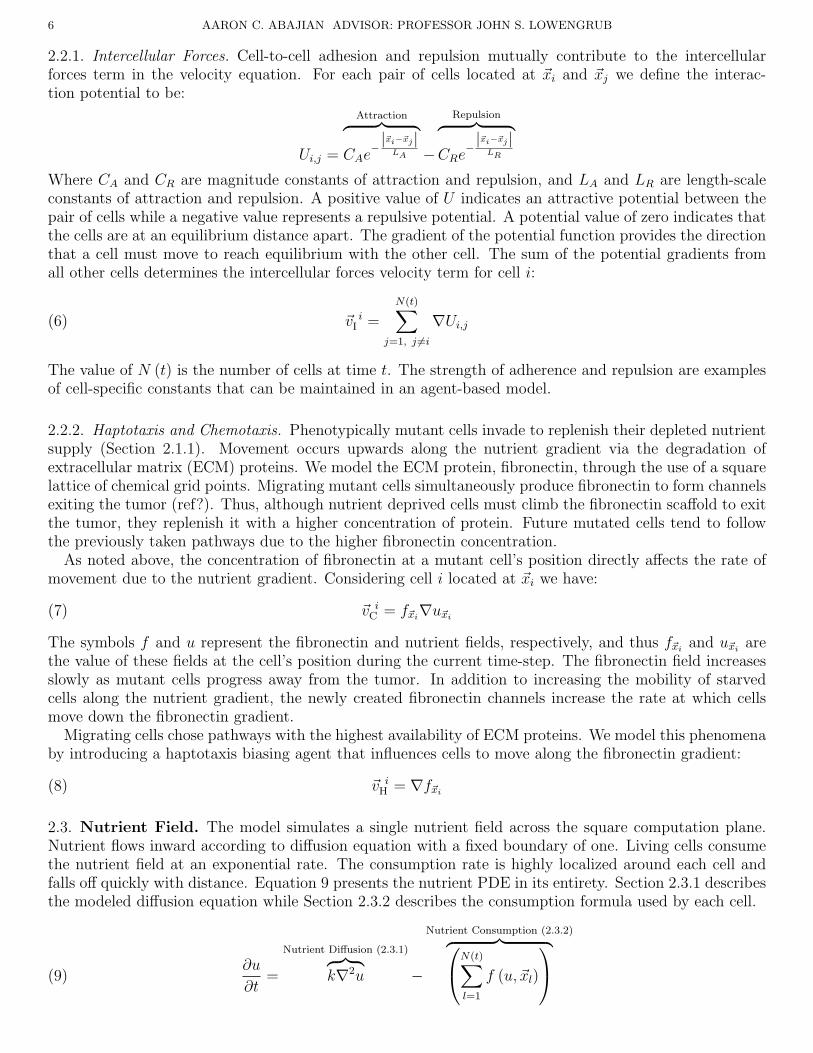
2.2.1. Intercellular Forces. Cell-to-cell adhesion and repulsion mutually contribute to the intercellularforces term in the velocity equation. For each pair of cells located at ~xi and ~xj we define the interac-tion potential to be:

Ui,j =

Attraction︷ ︸︸ ︷CAe

−|~xi−~xj|

LA −

Repulsion︷ ︸︸ ︷CRe

−|~xi−~xj|

LR

Where CA and CR are magnitude constants of attraction and repulsion, and LA and LR are length-scaleconstants of attraction and repulsion. A positive value of U indicates an attractive potential between thepair of cells while a negative value represents a repulsive potential. A potential value of zero indicates thatthe cells are at an equilibrium distance apart. The gradient of the potential function provides the directionthat a cell must move to reach equilibrium with the other cell. The sum of the potential gradients fromall other cells determines the intercellular forces velocity term for cell i:

(6) ~v iI =

N(t)∑j=1, j 6=i

∇Ui,j

The value of N (t) is the number of cells at time t. The strength of adherence and repulsion are examplesof cell-specific constants that can be maintained in an agent-based model.

2.2.2. Haptotaxis and Chemotaxis. Phenotypically mutant cells invade to replenish their depleted nutrientsupply (Section 2.1.1). Movement occurs upwards along the nutrient gradient via the degradation ofextracellular matrix (ECM) proteins. We model the ECM protein, fibronectin, through the use of a squarelattice of chemical grid points. Migrating mutant cells simultaneously produce fibronectin to form channelsexiting the tumor (ref?). Thus, although nutrient deprived cells must climb the fibronectin scaffold to exitthe tumor, they replenish it with a higher concentration of protein. Future mutated cells tend to followthe previously taken pathways due to the higher fibronectin concentration.

As noted above, the concentration of fibronectin at a mutant cell’s position directly affects the rate ofmovement due to the nutrient gradient. Considering cell i located at ~xi we have:

(7) ~v iC = f~xi

∇u~xi

The symbols f and u represent the fibronectin and nutrient fields, respectively, and thus f~xiand u~xi

arethe value of these fields at the cell’s position during the current time-step. The fibronectin field increasesslowly as mutant cells progress away from the tumor. In addition to increasing the mobility of starvedcells along the nutrient gradient, the newly created fibronectin channels increase the rate at which cellsmove down the fibronectin gradient.

Migrating cells chose pathways with the highest availability of ECM proteins. We model this phenomenaby introducing a haptotaxis biasing agent that influences cells to move along the fibronectin gradient:

(8) ~v iH = ∇f~xi

2.3. Nutrient Field. The model simulates a single nutrient field across the square computation plane.Nutrient flows inward according to diffusion equation with a fixed boundary of one. Living cells consumethe nutrient field at an exponential rate. The consumption rate is highly localized around each cell andfalls off quickly with distance. Equation 9 presents the nutrient PDE in its entirety. Section 2.3.1 describesthe modeled diffusion equation while Section 2.3.2 describes the consumption formula used by each cell.

(9)∂u

∂t=

Nutrient Diffusion (2.3.1)︷ ︸︸ ︷k∇2u −

Nutrient Consumption (2.3.2)︷ ︸︸ ︷N(t)∑l=1

f (u, ~xl)

AN AGENT-BASED HYBRID MODEL FOR AVASCULAR TUMOR GROWTH 7

2.3.1. Nutrient Diffusion. The nutrient concentration is replenished according to the diffusion equation intwo dimensions with a fixed square boundary:

(10) k∇2u = k

(∂2u

∂x2 +∂2u

∂y2

)The constant k determines the rate of nutrient influx. The diffusion rate of oxygen in water varies stronglywith temperature. At 20◦C, the coefficient k has been measured as 0.00197 mm2/s (ref?).

2.3.2. Nutrient Consumption. Cells consume nutrient at a rate that falls off exponentially with distance.The summation in Equation 9 is over the set of living cells at time t. Cell l consumes the local nutrientaccording to the following equation:

(11) f (u, ~xl) = −λe−|~x−~xl|

2

ε2 u

Where λ is the single-cell consumption rate, ~xl is the location of cell l as a function of time, and ε sets thedegree of localized nutrient consumption.

3. Numerical Methods

The agent-based modeling paradigm strongly supports an object-oriented implementation. We viewcells as self-contained entities with a fixed set of physical characteristics and functions (division, invasion,interactions, etc.). In an object-oriented programming language, information unique to a particular classof objects, such as cells, may be encapsulated and protected from external modification. We refer toimplemented classes using an italicized term with the first letter of each word capitalized to distinguishthem from their physical analogues (e.g. Cell refers to the class representing a physical cell). The processof instantiation creates an object of the respective class and allocates memory to store the new object’sdata. Thus, instantiation of the Cell class performs the necessary tasks to create a new cell. A completelist of the classes implemented in the model is provided in Table 3.1. Portions of the model implementedin each class are discussed in the section that follows.

The classes NutrientEquation, PotentialInteractions, and Fibronectin inherit operations from the moregeneral GenericField class. Inheritance is an important object-oriented programming concept that allowscode to be reused amongst similar classes. Its use in the model is described in Section 3.2.

The numerical tools used to implement the model were chosen based upon their running time efficiencyand ability to provide the desired object-oriented features. The model was written in C++ for rapidexecution and real-time visualization. MATLAB was used for partial postprocessing visualization. SeeSection 3.3 for further information.

Table 2. List of classes implemented in the model and their corresponding sections. Anobject-oriented implementation allows the encapsulation of data unique to a specific class ofobjects.

Class Section

TumorGrowth 3.1.1Cell 3.1.2Mitosis 3.1.2NutrientEquation 3.1.3Fibronectin 3.1.4DecayingFibronectin 3.1.4PotentialInteractions 3.1.5

3.1. Implemented Classes.

8 AARON C. ABAJIAN ADVISOR: PROFESSOR JOHN S. LOWENGRUB

3.1.1. TumorGrowth. The TumorGrowth class maintains an array of Cell objects that is initially populatedwith a single cell. The class controls execution of the model by calling functions to perform the actionspresented in the flow chart of Figure 1. Quick comparison calculations are carried out within TumorGrowthwhile more complex operations are located within their own classes (e.g. Mitosis, NutrientEquation, andPotentialInteractions).

Every time-step a subset of living cells from the cell array are selected for the calculation loop. Simulationresults indicate that it is sufficient to take log10 (N) cells where N is the size of the cell array. This isprimarily a consequence of the small time-step relative to the number of cells. In larger simulations, itwould be necessary to choose a greater subset of cells.

The selected cells are passed to an update function that updates that cell’s local nutrient concentrationand checks it against the nutrient thresholds. The cell’s quiescent, phenotypic mutation, and living booleanvariables are updated appropriately. Note that once a cell is marked as dead it is no longer a candidatefor the update function. The update function increments the cell’s age variable and checks for mitotic celldivision.

3.1.2. Cell and Mitosis. The Cell and Mitosis classes are strongly linked. After TumorGrowth verifies thata cell is ready to divide, it invokes an instance of Mitosis to perform the division. The division functioncopies all of the parent cell information and returns a new Cell object that is added to the array of cells.

3.1.3. NutrientEquation. The NutrientEquation class contains the numerical implementation of Equation9. The nutrient concentration is defined across a rectangular grid of points. During each time-step oflength t, nutrient diffuses across the nodes and cells consume from the nearby nodes. Discretization ofthe diffusion portion was accomplished using the central difference method. To begin the derivation ofthe nutrient concentration at node (i, j) and time-step n+ 1, we first rewrite the left-most and right-mostportions of Equation 9 as:

(12)un+1

i,j − uni,j

∆t= k

(∂2u

∂x2 +∂2u

∂y2

)n

− λN(n∆t)∑

l=1

e−|~xi,j−~xl(n∆t)|2

ε2 uni,j

Notice that we have substituted n∆t in for the continuous time t since we are assuming a fixed time-step.The superscript n on the continuous diffusion term just denotes that we are considering a discretizedtime-step.

The central difference method computes the gradient at a grid point by taking the average value ofthe gradient across the four nearest grid points. In particular, we may rewrite the continuous diffusionequation at time-step n as:

(13)

(∂2u

∂x2 +∂2u

∂y2

)n

=un

i+1,j − 2un+1i,j + un+1

i−1,j

∆x2+un

i,j+1 − 2un+1i,j + un+1

i,j−1

∆y2

Substituting this expression into that of Equation 12 produces the completely discretized nutrient equation:

(14)un+1

i,j − uni,j

∆t= k

(un

i+1,j − 2un+1i,j + un+1

i−1,j

∆x2+un

i,j+1 − 2un+1i,j + un+1

i,j−1

∆y2

)− λ

N(n∆t)∑l=1

e−|(i,j)−~xl(n∆t)|2

ε2 uni,j

The model uses a fixed spacing, h, between adjacent horizontal and vertical nodes so we have ∆x = ∆y = h.Equation 14 may be solved for the value of the nutrient concentration at grid point (i, j) and time-stepn+ 1:

(15) un+1i,j =

k(un

i+1,j + un+1i−1,j + un

i,j+1 + un+1i,j−1

)+ γun

i,j − λh2

N(n∆t)∑l=1

e−|(i,j)−~xl(n∆t)|2

ε2 uni,j

γ + 4k

Where: γ = h2

∆t, the initial nutrient concentration at each grid point is set to one: u (x, y, 0) = 1, and the

boundary is fixed at one: u (min (x) , y, t) = 1, (max (x) , y, t) = 1, (x,min (y) , t) = 1, (x,max (y) , t) = 1.

AN AGENT-BASED HYBRID MODEL FOR AVASCULAR TUMOR GROWTH 9

An object of the Nutrient class maintains a discrete field of nutrient grid points along with functions forupdating the field. Requests for evaluation at an arbitrary point on the computation plane are mappedto the nearest grid point. The competition between the influx of nutrient by diffusion and the removal ofnutrient by cellular consumption stabilizes after several iterations. Only grid points whose nutrient valueshave changed significantly (defined by a constant) are updated. A single pass over all the grid pointsidentifies those that have changed. The single pass is performed again after a set number of uptake cycleshave occurred. This algorithm was first introduced by Dr. Paul Macklin and decreases the time needed tosolve the discretized nutrient equation (ref?).

3.1.4. Fibronectin and DecayingFibronectin. The Fibronectin and DecayingFibronectin classes contain thenecessary routines to maintain and update the discretized fibronectin field. The implementation is identicalto that of the NutrientF ield class minus the diffusion functions. The Fibronectin class defines the under-lying grid while the DecayingFibronectin class contains functions that cells call to create or diminish thefield. The degradation and production functions for each cell are the same as Equation 11. Note, however,that the rate coefficients of nutrient degradation, fibronectin degradation, and fibronectin production aredistinct and that the production coefficient is negative.

3.1.5. PotentialInteractions. The task of calculating cellular interactions is passed off to a separate Poten-tialInteractions class. A member function of this class accepts a reference to the current cell array and aspecific cell index. The function iterates over the array and computes the summation given in Equation 6.The attractive and repulsive components are computed independently and preserved in separate arrays.This is necessary for the cell-repulsion check prior to mitosis (see Section 2.1.2).

3.2. Field Inheritance. The PotentialInteractions class inherits functions from the more general Gener-icField class. The Fibronectin and Nutrient classes also inherit from GenericField. It is worth describingthe structure of this inheritance to obtain a clear picture of the benefits of the object-oriented design ofthe model. Although the potential, nutrient, and fibronectin fields conceptually represent distinct entities,the physical definition of a field implies certain common characteristics.

The situation of having two similar objects that share synonymous functions, but with different im-plementations, arises quite often in computer science. Inheritance allows a general description of thecommonalities between the classes while maintaing enough room for separate implementations. Gener-icField provides function names for a physical field. Evaluation, the spatial partial derivatives, and the

Table 3. Functions defined in the GenericField class along with inheriting classes and themethod of each implementation.

Abstract Class GenericField

Function Implementing classes and type of implementation

f(x, y, z)PotentialInteractions Direct evaluation of Equation (6)Fibronectin

Discretized using the central difference methodNutrient

∂f

∂x,∂f

∂y,∂f

∂z

PotentialInteractions Continuous derivation from Equation (6)Fibronectin

Discretized using the central difference methodNutrient

|∇f | GenericField Implemented as

√(∂f

∂x

)2

+

(∂f

∂y

)2

+

(∂f

∂z

)2

magnitude of the gradient are defined in GenericField (see Table 3 for a complete list of functions definedin GenericField). In fact, the magnitude of the gradient is implemented in GenericField although thepartials themselves are not implemented. Inheriting classes must implement functions not implemented inGenericField (i.e. everything but the gradient magnitude), but a common naming convention is preserved.In this manner, it is a trivial task to define an array of GenericField objects whose actual instatiationsmay be any of PotentialInteractions, Nutrient, or Fibronectin.

10 AARON C. ABAJIAN ADVISOR: PROFESSOR JOHN S. LOWENGRUB

3.3. Implementation Tools. Standard computational tools were used to construct the model. An object-oriented framework was built from the ground up to support each cell as an autonomous unit. Theentire simulation was written in C++ with strict adherence to accepted best-practices in class design.Independent classes were constructed to maintain the functions and parameters of cells, fields, and otherdistinct entities within the model. Visualization was accomplished through an OpenGL-based display andframe-by-frame output. Cell data was also outputted as a text file containing each time-step. The latterenabled postprocessing visualization in MATLAB without the time-consuming process of concatenatingimage files. An (OpenGL-independent) simulation begins upon instantiation of the central TumorGrowthclass.

4. Numerical Results

The simulation parameters in Table 1 and Table 4 along with other parameters, such as those for thenutrient field and cellular interactions, determine the overall behavior of the tumor.

Table 4. List of global constants that determine the pathway of tumor development.

Global Constants

Variable Initial ValueMaximum number of cells ∞Computation window dimensions [−1, 1]× [−1, 1]Number of iterations ∞Time-step size 0.001Random number seed 1.000Quiescence nutrient threshold 0.600Living nutrient threshold 0.500Mutation nutrient threshold 0.510Repulsion maximum for division 2.000

A selection of these parameters were varied to understand their effects on the simulation. The fivevariables considered are provided in Table 5. Three thresholds exist that determine a tumor cell’s statusas normal, quiescent, mutant, or dead (see Figure 1). The images in Figures 2 through ?? represent thesestates as green, blue, black, and red, respectively. Phenotypic mutations were disabled in Figures 2, 3, and4 to focus upon the tumor at the stable necrosis stage prior to microinvasion.

Table 5. List of global constants that determine the pathway of tumor development.

Simulation Specific Constants

Variable Symbol Default ValuePotential attraction/repulsion coefficient ratio CA/CR 0.300Potential attraction and repulsion length-scales LA, LR 0.500, 0.100Quiescence nutrient threshold Tq 0.600Living nutrient threshold Td 0.500Mutation nutrient threshold Tm 0.510

4.1. Potential Coefficients. The potential coefficients and length scales are those given in Equation 6.The effect of the potential coefficients on the diameter of the tumor at a particular time-step is visuallydemonstrated in Figure 2. Similarly, Figure 3 shows the effects of the length scale on the tumor’s develop-ment. The tumor’s dimensions are largely determined by these four parameters. It is a requirement thatthe greater length-scale belong to the weaker force. This prevents implosion or indefinite expansion of thetumor.

AN AGENT-BASED HYBRID MODEL FOR AVASCULAR TUMOR GROWTH 11

4.1.1. Attraction to Repulsion Ratio. Increasing the ratio of attraction to repulsion increases the tendencyof cells to adhere to one another. Lower values of CA/CR produce larger tumors suitable for simulationsrequiring thousands of cells. High values constrict the cells together reducing the diameter of the tumor.The small diameter of the tumor precludes cell division because of the adjacency check prior to division(see Section 2.1.2). The decreased number of cells prevents depletion of the nutrient and provides for cellviability.

(a) CACR

= 0.1 (b) CACR

= 0.2 (c) CACR

= 0.3 (d) CACR

= 0.4 (e) CACR

= 0.5

Figure 2. Effect of attraction/repulsion ratio on diameter of tumor. The vertical axis issetup in one thousand time-step increments with the first row being at the thousandth step.Note that the length scales of attraction and repulsion have been set to 0.5 and 0.1, respec-tively.

12 AARON C. ABAJIAN ADVISOR: PROFESSOR JOHN S. LOWENGRUB

4.1.2. Attraction and Repulsion Length-Scales. The potential length-scale constants determine the effectiveradii of attraction and repulsion. The computation plane consisted of the unit-square and the repulsionlength-scale was fixed at one-tenth of this value. The left-most image of Figure 3 occurs when the length-scale of attraction equals that of repulsion. In this case, the tumor’s dimensions are determined by theratio of attraction and repulsion coefficients. The latter four images are similar because the attractionlength-scale strongly dominates the repulsion scale, although the magnitude of localized repulsion is stillgreater.

(a) LA = 0.1 (b) LA = 0.3 (c) LA = 0.5 (d) LA = 0.7 (e) LA = 0.9

Figure 3. Effect of increasing the length scale of attaction. The repulsion length scale wasfixed at 0.1 while the ratio of attraction to repulsion was set to 0.3. The images were takenat the five-thousandth time-step.

4.2. Nutrient Thresholds. The viability threshold figures were produced at the five-thousandth time-step as still frames from the graphical output.

4.2.1. Quiescence. In order to become quiescent, a cell must drop below the fixed Tq threshold. Figure 4shows the effects of increasing Tq on the tumor. The number of cells in the quiescent state increases withTq thereby determining the depth of the viable rim.

(a) Tq = 0.51 (b) Tq = 0.53 (c) Tq = 0.55 (d) Tq = 0.57 (e) Tq = 0.59

Figure 4. Effect of varying quiescent nutrient threshold, Tq, on tumor morphology.

4.2.2. Viability. Cells whose local nutrient concentration drops below the threshold for viability, Td, aremarked as dead. Figure 5 shows four simulations with increasing viability thresholds. A high viabilitythreshold decreases the time a cell may exist in the quiescent state. Thus, the number of quiescent cellsdiminishes rapidly as the necrosis threshold is increased.

4.2.3. Mutation. A subset of the cells that fall below the mutation threshold are made to undergo a micro-invasive mutation. Note that the mutation threshold, Tm, is less than Tq to ensure that the invadingcells are mitotically deactivated due to nutrient deprivation. Figure 6 shows the effects of increasing themutation threshold. The increasing mutation threshold decreases the number of necrotic cells since mutantcells are able to migrate away from the nutrient-deprived core.

AN AGENT-BASED HYBRID MODEL FOR AVASCULAR TUMOR GROWTH 13

(a) Td = 0.51 (b) Td = 0.53 (c) Td = 0.55 (d) Td = 0.57 (e) Td = 0.59

Figure 5. Effect of varying viability nutrient threshold, Td, on tumor morphology.

Over time, the mutant cells break the adhesive forces binding them to the other cells and move awayfrom the tumor along fibronectin and nutrient gradients. Figure 4.2.3 shows a longer simulation at thefourty-thousandth time-step. The darkened paths were produced by interpolating the fibronectin gridpoints across the pixels of the figure. The darker lines indicate a high fibronectin concentration.

(a) Td = 0.51 (b) Td = 0.53 (c) Td = 0.55 (d) Td = 0.57 (e) Td = 0.59

Figure 6. Effect of varying mutation nutrient threshold, Tm, on tumor morphology.

Mutant cells degrade and produce the local fibronectin concentration. Production is the dominatingprocess and thus mutant cells create pathways of high fibronectin as they leave the tumor. Later mutantstend to exit the tumor along these preformed paths [2].

Figure 7. A fraction of viable cells below the mutant threshold are selected to undergo aphenotypic mutation. These cells move away from the tumor up the nutrient gradient. Eachcell produces a local fibronectin field that also biases the motion of future mutants. Thistype of migration is termed micro-invasion and is believe to be a response to nutrient depri-vation.

14 AARON C. ABAJIAN ADVISOR: PROFESSOR JOHN S. LOWENGRUB

5. Conclusion

An extensive range of processes participate in tumor development. The three generalized phases of tumorgrowth include the initial single-cell genetic mutation and exponential division, formation of a circularmass with a central necrotic region and a proliferating rim, and invasion on either a micro or macro level.Chemotherapeutic treatment options focus upon the rampant proliferation and consumption associatedwith invasive tissue. The question of appropriate medicinal dosage rests upon the rate of abnormal drugconsumption compared to the basal consumption rate. We have introduced a computational model foravascular tumor growth that simulates the essential competition between diffusive nutrient influx andcellular nutrient uptake witnessed in a variety of tumors.

The model maintains individual cell data in an agent-based fashion while incorporating features ofcontinuos models to allow for nutrient flow. This structure provides unique insight into the pathway tonecrotic core formation and micro-invasion, especially in regards to competitive nutrient depletion. Themodel demonstrates a clear transition from a fully viable spherical mass to the commonly observed three-tiered tumor (i.e. viable rim, quiescent region, and necrotic core). The model’s parameters determinethe width of these regions at the stability stage prior to invasion. The magnitude and length scales ofattraction and repulsion affect the overall size of the tumor while the nutrient thresholds specify theminimum concentration of resources necessary for viability, mutation, and quiescence.

Although future work is necessary to determine the appropriate constants for specific cases, the modelfunctions well as an initial tumor development framework. A substantive improvement would be theintroduction of independent nutrient and chemical fields that influence cellular behavior. Immersion of thetumor model into such a simulated microenvironment that includes normal cells would provide immediatepredictive ability about the appropriate substance concentration to establish a particular level of necrosis.The model is well adapted to this endeavor through its object-oriented implementation of cells and diffusivefields.

References

[1] Yao li Chuang, Maria R. D’Orsogna, Daniel Marthaler, Andrea L. Bertozzi, and Lincoln S. Chayes. State transitions andthe continuum limit for a 2D interacting, self-propelled particle system, 2006.

[2] Hans G. Othmer and Angela Stevens. Aggregation, blowup, and collapse: the ABC’s of taxis in reinforced random walks.SIAM J. Appl. Math., 57(4):1044–1081, 1997.

[3] American Cancer Society. Cancer facts & figures 2007. none, 2007.